
Politics and violence are inextricably linked. No contemporary political group highlights this connection more clearly than the Islamic State in Iraq and Syria (ISIS), which has beheaded journalists, massacred minority groups, and glorified these exploits with videos that have spread throughout the world via the Internet.Footnote 1 The group's extreme use of violence has led some to conclude that their actions are driven by a violent ideology, rather than by strategic motivations.Footnote 2 Others argue that ISIS uses violence in an instrumentally rational manner, potentially to draw international attention and recruits, or to force local populations into submission.Footnote 3
The question of whether ISIS's use of violence is driven by ideological motivation or strategic logic parallels the two major schools of thought in the academic study of conflict. Strategic (“rationalist”) theories often employ game-theoretic models and examine how violence is used for instrumental purposes.Footnote 4 In this approach, leaders use violence to increase or maintain their power and people participate in violence in exchange for selective or material gain. Seemingly in contrast, psychological explanations posit that political violence is primarily driven by emotional or identity grievances, ethnic or religious hatred, or in defense of sacred values.Footnote 5
Scholars of the strategic and psychological schools of conflict have critiqued each other's approach as overly simplistic or as lacking explanatory power. Critics of strategic models question “the conceptual worth of assigning, for example, a hate-filled action a certain participatory ‘utility’ or ‘value’ when the emotion of hate itself is the driving and determinative force.”Footnote 6 Critics of psychological theories can be equally harsh, for example, claiming that “however appealing to one's intuition such explanations seem, there is nothing in the logical structure of the psychological theories from which such hypotheses were derived to indicate that frustrated individuals, in their capacities as national leaders, particularly vent their frustrations (or aggression) by the use of military force.”Footnote 7
We argue that the divide between strategic and psychological explanations for conflict is artificial.Footnote 8 To support this argument, we develop a formal model that loosens a commonly critiqued assumption of bargaining models and standard game-theoretic approaches more generally—that the actors' preferences over agreements and fighting are fixed and exogenous.Footnote 9 We adopt an “indirect evolutionary” approach in which actors behave rationally given their preferences, but their preferences are subject to evolutionary forces. This is (to our knowledge) the first paper to use an indirect evolutionary approach in international relations or political science more broadly.
Our argument builds on a fundamental insight from Thomas Schelling: that willingness to reject unfavorable offers that are still preferable to no agreement can confer an advantage in bargaining.Footnote 10 As expressed in our model, if the preferences of actors in a bargaining scenario are derived from an evolutionary process, those with “irrationally tough” preferences can attain higher fitness. The actors develop preferences that make them more willing to fight than is assumed in standard bargaining models. Put another way, not only is the strategic environment for those who fight and bargain shaped by their preferences, but their preferences are also shaped by the strategic environment.
We model the evolution of preferences in the following fashion. In each generation, the actors play a standard bargaining game where a proposer makes an offer to divide a prize that a responder can accept or reject. If the responder rejects, the actors fight over the prize. The key innovation is that we allow the actors' preferences over deals and conflict—which determine their behavior—to diverge from their fitness, (or objective payoffs) which determines their evolutionary success. Those whose preferences lead them to bargain in a manner that yields a greater fitness are more successful and their preferences become more common in the next generation. In particular, the next generation's preferences are given by the preferences of their “parents,” plus a random perturbation. A solution to the model is a set of preferences and strategies such that the strategies are optimal given the players' preferences, and the distribution of preferences given this reproduction process remains stable across generations.
Unlike nearly all standard bargaining models of war, we find that for any cost of conflict (and other parameter values), every equilibrium must have conflict. To see why, imagine a world where fighting never occurs. When bargains are always reached, being tougher always leads to better deals and hence confers a particularly powerful fitness advantage. Further, in this fully peaceful world, developing a greater taste for fighting has no downside since the fitness loss from conflict is never realized.Footnote 11 Evolutionary forces therefore make the next generation tougher. And if this new generation also never fights, subsequent generations must continue to become tougher until conflict does occur.
More generally, for a preference distribution to be stable, those with “average” toughness must get the highest fitness.Footnote 12 Conflict must sometimes occur to prevent the toughest types from being the most fit. Conversely, when conflict is extremely common, the weakest types who are sometimes able to strike deals attain the highest fitness and reproduce more.
Evolutionary forces push the population to a unique stable preference distribution where the average toughness and probability of conflict are just high enough that a typical member of the population bargains most successfully. Analyzing the preferences and behavior in this equilibrium allows us to shed new light on major theoretical and empirical debates in international relations by examining how factors like the costliness of fighting affect both how tough the players are in the stable distribution, and the frequency of conflict given these preferences.
A central result of our main model—which again contrasts with bargaining models of war with fixed preferences—is that even as fighting becomes arbitrarily costly, the probability of fighting does not become (or even approach) zero. This is because conflict becoming costlier makes others more reluctant to fight, allowing tougher bargainers to extract better deals. We tie these results to debates about how technology that makes conflict more destructive (e.g., nuclear weapons) affects the likelihood and expected costs of war,Footnote 13 as well as notable recent claims about the decline of violence throughout human history.Footnote 14
We then loosen the assumption that preferences are common knowledge, providing a new perspective on the question of how uncertainty affects the possibility of conflict. In line with standard models, we find that adding incomplete information leads to more conflict for fixed preferences. However, when preferences are harder to observe, the evolutionary advantage to being tough decreases, which can lead to players developing dovish preferences. So the probability of conflict in the stable preference distribution is often lower when it is harder to assess the type of bargaining partners. These results suggest that any new technology that makes it easier to know the preferences or capabilities of bargaining opponents will reduce the likelihood of conflict in the short term but could potentially increase the prevalence of conflict in the long term.
By showing that origins of conflict may lie in both nonmaterial preferences and strategic behavior, we bridge the bargaining literature on conflict with empirical and theoretical insights from psychology for nonmaterial motivations for behavior. Our approach provides new insights into a wide range of major debates about what factors make conflict more or less likely. A common thread to the empirical implications of our approach is that changes to military technology or the international system—which affect, for example, the cost of fighting or the visibility of opponents' capabilities or resolve—may have different effects in the short term (before preferences can adjust) versus in the long term (when preferences evolve). Although the standard approach of treating preferences as exogenous has been successful at generating tractable and influential models, it may lead to incorrect inferences about the long-run determinants of war.
Related Work
The main puzzle motivating bargaining theories of war is that if conflict is costly, then participants should be able to find an agreement that both prefer to fighting. In one of the most prominent papers to frame interstate war in this light, James Fearon identifies two principal reasons for costly conflict even when there are ex ante agreements preferable to fighting: information asymmetries and commitment problems.Footnote 15 This bargaining approach has generated a large and successful literature on how conflict may result from (among other forces) domestic politics,Footnote 16 changes in the balance of power,Footnote 17 or mutual optimism.Footnote 18
As with standard game-theoretic analysis, this work takes the bargainers' preferences as fixed. The bargaining approach also typically assumes that these preferences allow for peaceful agreements that all prefer to fighting (a “bargaining range”). However, many empirical and theoretical studies in psychology have critiqued this approach by highlighting how actual behavior deviates from the predictions of standard game-theoretic models of conflict.Footnote 19 For example, emotions stemming from past interethnic violence serve as impediments to peaceful resolutions to present-day conflicts.Footnote 20 Experimental research further suggests that highly committed individuals put more weight on moral or deontological concerns, as opposed to instrumental concerns (costs of conflict, probability of success, etc.) when deciding whether to bargain or fight.Footnote 21 While a central contribution of the theoretical bargaining literature has been to show that conflict may occur even without these considerations, this does not imply that “psychological” reasons for conflict should be ignored. In fact, there is good reason to suspect that nonmaterial motivations drive much of the variation in violence that we observe among individuals and groups.Footnote 22
Closest to our model, many experimental studies of the “ultimatum game” and related models find that individuals are willing to reject offers that would lead to a higher material payoff. This willingness to forego resources arises out of a desire for fairness, identity concerns, or other nonmaterial incentives.Footnote 23 Much of this work draws on convenience samples (e.g., college students), who may bargain differently than leaders making consequential decisions about war and peace. However, more recent experiments find that elites with experience in making foreign policy exhibit similar biases,Footnote 24 and in fact may be more willing to reject unfavorable offers in bargaining games.Footnote 25 Since rejecting offers entails conflict in bargaining models of war, these findings suggest that the notion of conflict driven by actors with non-instrumental motivations should not be dismissed lightly.Footnote 26
Our approach shows how such behavioral biases can not only be incorporated into the bargaining framework,Footnote 27 but also arise endogenously from a bargaining framework where preferences are subject to evolutionary forces. We begin with a canonical bargaining model where conflict would not happen using a standard solution concept, and find that as a consequence there are not always agreements that are mutually preferable to conflict given the players' endogenously derived preferences.
To formalize the origin of preferences, we use an indirect evolutionary approach.Footnote 28 The “indirect” qualifier differentiates our approach from “direct” evolutionary models where strategies are not consciously chosen by players but determined by evolutionary forces. In indirect evolutionary models, actors choose optimal strategies given their preferences, but evolutionary forces shape the actors' preferences, indirectly affecting their behavior. Past work has used “direct” evolutionary game theory to gain insights into interpersonalFootnote 29 and interstate conflict,Footnote 30 but these models do not allow the actors to bargain before fighting, making it difficult to relate the results to the standard formal models to war.
Our approach is designed precisely to ameliorate this shortcoming. By jointly modeling the formation of preferences and bargaining behavior, we formalize the idea that evolutionary forces can favor those with preferences that make them “irrationally” tough while retaining the standard game-theoretic assumption that the actors behave optimally given their preferences. Equally important for the question at hand, we also retain the central premise of the bargaining literature that conflict is costly and inefficient from an objective perspective.
We let preferences diverge from fitness payoffs in a simple and easy-to-interpret way, by allowing the actors to assign a higher (or lower) subjective utility to fighting than their fitness associated with this outcome.Footnote 31 We call the degree of divergence from the objective payoff associated with fighting “toughness.”Footnote 32 Within the indirect evolution literature, our model is most closely related to Heifetz and Segev's model of evolutionary preferences over the value of goods in market bargaining.Footnote 33 However, our model differs in both focus and execution. We are more concerned with the possibility of conflict—or, equivalently, the breakdown of bargaining—than the bargaining itself. In particular, we relate and structure our model in line with the extant political science literature on conflict and war, not bargaining among buyers and sellers where it is natural that there is not always a price acceptable to both parties. In terms of execution, we explicitly model the noise in the evolutionary process, which has important consequences for studying conflict.Footnote 34 Our model is therefore more directly related to understanding the evolved nature of emotions since the behavioral traits that influence emotions are the result of a “noisy” evolutionary process.Footnote 35
Incorporating these insights into a formal model challenges several main findings from the bargaining approach to war. First, we find that conflict must occur in every equilibrium even with complete and perfect information.Footnote 36 Second, not only is the probability of conflict always positive, but in our main model it does not even approach zero as the cost of conflict gets very large, as in most canonical models.Footnote 37 Finally, we find that introducing incomplete information, which is widely considered to be a main cause of war,Footnote 38 can decrease the probability of conflict.
An Illustration
To illustrate the logic behind many of the results to come, we first present a highly stylized example. The general mechanisms in this illustration are similar to the “hawk-dove” game commonly used in the evolutionary game theory literature,Footnote 39 though with payoffs and an interpretation arising from a bargaining situation to connect to our main analysis.Footnote 40
Suppose there is a large population of individuals who are randomly paired with a partner and bargain over how to divide a dollar. There are two “types” of people, relatively tough types (analogous to “hawks”) and relatively weak types (analogous to “doves”).Footnote 41 When two of the weak types are matched with each other, they split the dollar evenly and both get a fitness of 1/2. When a tough and weak type are matched, the tough type exploits the weak type, taking 1/2 + δ of the dollar and leaving 1/2 − δ to the weak type, where 0 < δ < 1/2. So, δ represents the level of exploitation. When two tough types are matched, they are unable to reach an agreement (alternatively, they “fight”) and both get a fitness of 0.
Aggregate welfare would be highest if all were weak types and split the dollar evenly. However, this arrangement is not “stable,” in the sense that tough types could enter this society and exploit everyone with whom they bargain. Conversely, if society is almost entirely populated by tough types, weak types would do better because the fitness from getting exploited (1/2 − δ) is higher than the fitness from fighting (0). In general, when the population includes very few tough types, it pays to be tough, and when there are many tough types it is better to be weak. This results in a unique proportion of tough types (and corresponding probability of conflict) that are stable, in the sense that both types get the same fitness.
Formally, if the proportion of tough types is p h , then the average fitness for being a weak type is (1 − p h )(1/2) + p h (1/2 − δ). The average fitness for being a tough type is (1 − p h )(1/2 + δ) + p h 0. So, if
 $$1/2 - p_h \delta = (1 - p_h )(1/2 + \delta ) \Rightarrow p_h = 2\delta, $$
then the weak and tough types are equally well off. When p h < 2δ, tough types get a higher fitness, so we may expect their share of the population to grow (i.e., p h will increase). When p h > 2δ, the weak types get a higher fitness by avoiding conflict. In this situation, we would expect the population of weak types to grow (i.e., p h will decrease). So p h = 2δ constitutes a stable distribution of weak and tough types. (Since 0 < δ < 1/2, this proportion of tough types is always between 0 and 1.)
Since conflict occurs when two types are matched, the probability of conflict in the stable distribution is
 $p_h^2 = 4\delta ^2 $
, which can also range from 0 to 1. In particular, when δ is low (i.e., there is little exploitation), most players will be the weak types and little conflict will occur. When δ is high, conflict nearly always occurs. Thus the likelihood of conflict is a direct result of the underlying distribution of individuals with a propensity to fight.
The results we derive in more complex settings share some of the key qualitative properties as this simple example. First, there is a trade-off in being tougher, which is analogous to the risk-reward trade-off in incomplete-information bargaining games: tougher types get better bargains conditional on a bargain being struck, but also face a higher chance of inefficient fighting. Second, when a population exhibits a low degree of toughness the tough types tend to be more fit. When there is a high degree of toughness the weak types do better, which leads to a stable proportion of tough types when all are equally well off. Third, in this stable configuration, conflict occurs even though each player would have been better off getting exploited.
The Bargaining Game
The core of our model is a canonical two-player take-it-or-leave-it bargaining game. The players bargain over a prize with value normalized to 2v > 0. Player 1 (the “proposer”) makes an offer x, which corresponds to the amount of the prize going to player 2 (the “responder”), and player 2 can accept or reject the offer. To avoid dealing with boundary issues, let x ∈ ℝ.Footnote 42 If the responder accepts, the prize is divided as proposed (2v − x, x). If the responder rejects, there is a conflict over the division of the prize. When conflict occurs, each player “wins” and obtains the entire prize with probability 1/2, so the expected share of the prize from fighting is v. Conflict is costly, imposing a cost of k > 0 to each player. So the expected resources from fighting are v − k.
For now we remain agnostic about who the players are, for example, individuals, groups, or states. We also remain agnostic about what conflict entails (a potentially lucrative deal not being made, a minor skirmish over resources, major war), other than assuming that conflict imposes a cost on both actors. We revisit the implications of these various interpretations throughout our analysis and discussion.
The main innovation in our model is that each player also has some level of “toughness.” This toughness affects the players' subjective preferences (and hence behavior) for conflict but not their fitness (or objective payoff), which determines evolutionary success. As Table 1 summarizes, we assume the fitness payoffs match the share of the resources derived from the bargaining process. Further, for the cases where a deal is reached, the actors' preferences are equal to their fitness. However, we assume the preferences over the conflict outcome are v − k + β j for some β j ∈ ℝ. That is, types with β j > 0 are more willing to fight than their objective fitness would dictate. Since a higher β j increases the preferences over fighting, we refer to types with high β j as tough or high types, contrasted with weak or low types. To be clear, this “toughness” is in the subjective utility from conflict only and not being objectively better at fighting because again we assume any conflict is won by both players with equal probability.Footnote 43 Our concept of toughness is closely related to the idea that individual variation in emotionality (particularly anger) serve as commitment devices, leading to credible threats.Footnote 44
Preferences and fitness in the bargaining model

First we analyze how the players behave given their preferences by identifying the Subgame Perfect Nash Equilibra (SPNE) of the model. The objective payoffs will influence how preferences evolve in our main models.
Using backwards induction, the responder (player 2) accepts the offer if and only if x ≥ v − k + β 2. The proposer's subjective utility is strictly decreasing for offers higher than this, so they either offer exactly x = v − k + β 2 or make some lower offer, knowing it will be rejected. The proposer prefers to make the offer large enough to avoid conflict if and only if they prefer keeping 2v − (v − k + β 2) to their conflict utility:
 $$2v - \left( {v - k + \beta _2} \right) \ge v - k + \beta _1 $$
 $$\beta _1 + \beta _2 \le 2k$$
That is, if the aggregate level of toughness is sufficiently high that there is no mutually beneficial bargain in terms of subjective preferences, the two players fight. Otherwise, they strike the bargain determined by the responder's reservation point.
Lemma 1
For fixed and known types β 1, β 2:
i) If β 1 + β 2 ≤ 2k, there exists a unique SPNE where the proposer offers v − k + β 2 and the responder accepts this (and any higher offer).
ii) If β 1 + β 2 >2 k, then a strategy profile is an SPNE if and only if the proposer offers x < v − k + β 2, the responder rejects any offer less than v − k + β 2, and the equilibrium outcome is conflict.
Proof
Proof follows from the analysis.
Why an Indirect Evolutionary Approach?
Next we model how the players' preferences evolve. Our formal analysis could represent evolutionary forces on several actors on several levels, and we do not take a hard stance on which is “correct” interpretation.
The most natural interpretation of the model is one of interpersonal conflict where success in day-to-day interactions with others affects reproductive success. The idea that the ability to manage conflict is an important trait driving evolutionary success enjoys wide theoretical and empirical support.Footnote 45 Since conflict over resources is not limited to modern-day individuals, the way that our ancestors handled a wide variety of interactions with others could shape the way we think about bargaining today. Under this interpretation the evolutionary process is slow, and may not respond quickly to changing environments, which has important consequences for our comparative static analysis. However, other forms of adaptation and learning on the individual level could change more quickly. For example, it may be the case that those who grow up in more violent societies develop tougher “personas” as a result of preference evolution.Footnote 46
At a state level, as previous evolutionary approaches to international relations argue, different internal political or cultural factors affect (or select) how aggressive leaders are in bargaining, and more successful political systems will proliferate more than failed ones, either through survival or learning.Footnote 47 Further, if a country with an aggressive or nationalistic leader is successful on the international front, domestic constituencies in other countries may be more apt to choose an aggressive leader as well.
Individual- and state-level evolutionary forces can also interact. Leaders who make decisions about war and peace have preferences for bargaining over major issues that could reflect how they view bargaining and compromise more generally.Footnote 48 Further, leaders who are socialized in different circumstances, such as serving in the military,Footnote 49 leading a revolutionary movement,Footnote 50 or being raised in a “culture of honor”Footnote 51 have been shown to have different propensities to fight. In this case, the selection process may be orthogonal to (or precedes) the actual fighting, yet shapes the characteristics of leaders, or the winning coalition that wishes to choose “aggressive” types. That is, a cultural predisposition to aggression arising from interpersonal interactions spill over into foreign-policy decision making.
The constituents who select leaders and may hold them accountable (whether the inner circle of a dictator or the public in a democracy) also have preferences shaped by evolutionary forces that may lead them to be accepting of conflict or dislike compromise,Footnote 52 particularly over issues that become “moralized.”Footnote 53 That is, if both citizens and leaders are generally biased toward fighting, then regardless of the specific ways in which leaders are chosen or removed we should expect to see these biases show up in the decisions that leaders make. Of course, different countries have different institutional features that affect what kinds of leaders are chosen, which leads back to the argument that institutional heterogeneity can also be an alternative mechanism for the “evolutionary” forces we analyze.
Preferences must come from somewhere. While the traditional game-theoretic approach of treating preferences as given is a reasonable modeling assumption that has generated a rich literature in the study of conflict, we view breaking this assumption as an important innovation. Using an evolutionary approach to model the origin of preferences is theoretically coherent, leads to results consistent with a wide variety of experimental work, and challenges some of the key findings from models that treat preferences as fixed.
Analysis with Evolutionary Preferences
Our solution concept formalizes the following iterated process. First, a population with an initial distribution of toughness F(β) plays the bargaining game, and each actor's expected fitness is computed. We write the expected fitness for an actor with type β j when matched with a player with type β −j and playing the bargaining game with strategy profile σ as π(β j ; β −j ; σ). The expected fitness for an actor with type β j when matched with a population with toughness parameters following a distribution F and playing strategy profile σ is then:
 $$\Pi (\beta _j ;F;\sigma ) = \,{\int}\, \pi (\beta _j, \beta _{ - j} ;\sigma )dF(\beta _{ - j} )$$
Our most general result assumes that types that get a higher fitness reproduce at a faster rate, and that the next generation's toughness is a function of the parents' toughness plus noise with weak distributional requirements. However, to derive clear results in a relatively straightforward fashion, our main analysis makes stronger assumptions. In particular, let β max (F) be the type that gets the highest fitness when the initial preference distribution is F and the strategies used are the SPNE identified in lemma 1. We assume that the next-generation distribution of toughness is uniformly distributed on [β max (F) − ε, β max (F) + ε], where ε > 0 represents the degree of noise in the evolutionary process. A distribution of preferences is stable if the next-generation distribution of toughness matches the initial distribution.
That is, we assume that (1) only the types with the highest fitness in a generation reproduce, and (2) the toughness of the next generation is equal to the type that attained the highest fitness in the previous generation plus uniform noise. So a distribution of preferences is stable across generations if and only if type β* gets the highest fitness when the population is uniformly distributed on [β* − ε, β* + ε].Footnote 54
To solve for a stable β*, we first compute the expected fitness for having toughness β j when the population toughness is uniformly distributed on [β m − ε, β m + ε]. There are three key cases to consider.
First, sufficiently tough types (β j > 2k − (β m − ε)) fight even the least tough members of the population, giving fitness v − k.
Second, sufficiently weak types (β
j
< 2k − (β
m
+ ε)) will strike a deal with everyone in the population. So, when in the responder role these types attain fitness v − k + β
j
, and when in the proposer role their average fitness is v + k − β
m
. The total expected fitness is then
 $v + \displaystyle{{\beta _j - \beta _m} \over 2}$
. This is increasing in β
j
, because for those who never fight, it is best to be as tough as possible. Without facing the fitness loss from engaging in costly conflict, the better deals attained by having a strong taste for fighting always lead to higher fitness.
Finally, types with toughness between 2k − (β
m
+ ε) and 2k − (β
m
− ε) will fight with the tougher members of the population and strike a deal with weaker types. In particular, if β
−j
> 2k − β
j
, which occurs with probability
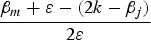 $\displaystyle{{\beta _m + {\varepsilon} - (2k - \beta _j )} \over {2{\varepsilon}}} $
, there is conflict that gives fitness v − k. With complementary probability, a deal is struck. When in the responder role this gives fitness v − k + β
j
, and when in the proposer role, the average fitness is
 $v + k - {\rm {\opf E}}[\beta _{ - j} \vert \beta _{ - j} \lt 2k - \beta _j]$
. So for types that sometimes fight, the expected fitness is:
 $$\underbrace {\displaystyle{{2k - \beta _j - (\beta _m - { \varepsilon} )} \over { 2\varepsilon}}} _{Pr({\rm deal})}\underbrace {\left( {v + \displaystyle{{\beta _j - (2k - \beta _j + \beta _m - {\varepsilon} )/2} \over 2}} \right)}_{\rm{expected \;\;fitness \;\;from \;\;deal}} + \underbrace {\displaystyle{{\beta _m + {\varepsilon} - (2k - \beta _j )} \over {2{\varepsilon}}}} _{Pr({\rm conflict})}\underbrace {\left( {v - k} \right)}_{\rm{conflict \;\;fitness}}\!\!.$$
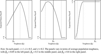
Figure 1 shows several illustrative cases of the fitness function for different toughness distributions. In each panel, the solid vertical line corresponds to the mean of the toughness distribution (β m ), and the dotted lines are at 2k − (β m + ε) and 2k − (β m − ε). Types with a toughness to the left of the first dotted line always reach a bargain, and the fitness is increasing in this range as it leads to better deals without conflict. Types to the right of the second dotted line always fight, giving a constant fitness v − k. Types between the dotted lines strike a deal with the relatively weak types and fight against the relatively tough types. The difference between the panels is in β m , which is low in the left panel, intermediate in the middle panel, and high in the right panel.
Expected fitness as a function of toughness for uniformly distributed populations.

Recall that the toughness of the next generation is centered on the type attaining the highest fitness in the current generation, that is, the maximum of the expected fitness function. The location of this maximum depends on what happens in the middle section, corresponding to types that sometimes but not always fight. In the left panel, the expected fitness function is always decreasing in toughness on this middle interval. This is because when β m is low, one can strike good deals even with the toughest types, so the fitness loss from fighting even the most difficult bargaining partners outweighs the gains from being tougher. In this case, the toughest type that never fights attains the highest fitness. However, the type attaining the highest fitness is above β m , indicating that the preference distribution is not stable.Footnote 55
In the right panel, the population is so tough that any possible bargain is worse than fighting and so there is no optimal toughness. As we discuss in the appendix, there is no distribution of types where conflict occurs and is stable in this contingency.Footnote 56
In the middle panel, β m is intermediate. As a result the optimal level of toughness occurs with a type that sometimes fights (i.e., between the dotted lines). In particular, the better deals earned from being tough enough that bargaining sometimes breaks down outweigh the cost of fighting when this occurs. However, as β j increases and the probability of fighting increases, the marginal benefit from getting better deals decreases. Here the point where the marginal benefit to getting better deals is offset by the increased chance of fighting—that is, the peak of the fitness function—is less than β m , so this distribution of preferences is not stable either.
In general, when β
m
is low, the type attaining the highest fitness is the toughest one who does not fight, and when β
m
is high the fittest type is one that sometimes fights. This type is located at the maximum of the second segment that occurs at
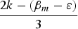 $\displaystyle{{2k - (\beta _m - { \varepsilon} )} \over 3}$
:
 $$\beta _{{\rm max}} (\beta _m ) = \left\{ {\matrix{ {2k - (\beta _m + { \varepsilon} )} \hfill & {\beta _m \lt 2k - 2{\varepsilon}} \hfill \cr {\displaystyle{{2k - (\beta _m - { \varepsilon} )} \over 3}} \hfill & {\beta _m \in (2k - 2{\varepsilon}, 2k + {\varepsilon} )} \hfill \cr}} \right.$$
The optimal level of toughness on both segments is increasing in k. This may be surprising: when conflict becomes more costly, we might expect that it would be advantageous to develop an aversion to fighting to avoid incurring the higher cost. However, this intuition ignores a key aspect of the strategic nature of bargaining situations: when conflict becomes costlier the other player also increasingly wants to avoid fighting. When the other player becomes more averse to fighting, the value of being tough to achieve better deals becomes larger.
Recall a stable preference distribution is centered on a β* such that β* = β max (β*). Plugging this into equation (1) gives us:
Lemma 2
In the model with uniform noise, for any k and ε, there is a unique stable distribution of preferences which is uniform on [β* − ε, β* + ε], where:
 $$\beta ^{\ast} = \left\{ {\matrix{ {\displaystyle{k \over 2} + \displaystyle{{\varepsilon} \over 4}} & {k \lt \displaystyle{3 \over 2}{ \varepsilon}} \cr {k - \displaystyle{{\varepsilon} \over 2}} & {k \ge \displaystyle{3 \over 2}{ \varepsilon}} \cr}} \right.$$
The likelihood of conflict in the stable preference distribution is the probability that the sum of the toughness levels is greater than 2k. When the toughness levels are uniform, the sum of the toughness levels β j + β −j follows a triangle distribution, and the probability of conflict in the stable preference distribution is:
 $$Pr(\beta _j + \beta _{ - j} \gt 2k) = \left\{ {\matrix{ {1 - \displaystyle{{(k + \displaystyle{3 \over 2}{\varepsilon} )^2} \over {8{\rm \varepsilon} ^2}}} & {k \lt { \varepsilon} /2} \cr {\displaystyle{{(k - \displaystyle{5 \over 2}{ \varepsilon} )^2} \over {8{\varepsilon} ^2}}} & {k \in \left ({\varepsilon} /2,\displaystyle{3 \over 2}{ \varepsilon} \right) } \cr {1/8} & {k \ge \displaystyle{3 \over 2}{ \varepsilon}} \cr}} \right.$$
(See the appendix.)
Taking the comparative statics on the average toughness and probability of conflict in the stable distribution of preferences gives us our first main results:
Proposition 1
In the stable distribution of preferences for the single-reproducer model with uniform noise:
i) the average toughness of the players is increasing in k, and increasing in ε if and only if
 $k \lt \displaystyle{3 \over 2}{\varepsilon} $
; and
ii) the probability of conflict is decreasing in k, increasing in ε, and at least 1/8.
Part (i) states that the stable configuration of preferences is more belligerent when conflict is more costly. We elaborate on the intuition soon. Part (ii) of proposition 1 states that with uniform noise in the evolutionary process, there is no equilibrium without conflict because the absence of conflict is unstable. In a fully peaceful society, the toughest types would reproduce in greater numbers, creating even tougher types. There must be some deterrent to developing a taste for fighting, and inefficient conflict is the only possible source of such deterrence. Thus, conflict is inevitable. No matter how costly conflict is or how small the noise in the evolutionary process, there is a lower bound on the probability of conflict, which in the case of uniform noise is one eighth of interactions (we later illustrate this origin of this particular fraction).
In a sense, part (ii) of proposition 1 is a stronger prediction than many canonical results about how conflict can arise in bargaining games. For example, many results require that bargainers are sufficiently impatient or the shocks to relative power are sufficiently large,Footnote 57 the information asymmetry is sufficiently large or the cost of conflict sufficiently low,Footnote 58 or they show only the existence of an equilibrium with conflict while a peaceful equilibrium exists as well.Footnote 59 Here every equilibrium has conflict.Footnote 60
Comparing parts (i) and (ii), this result also sheds light on the prominent arguments about the decline of various types of violence over time. Pinker argues that conflict has become more costly (or less beneficial) over time, and as a result people have become more peaceful.Footnote 61 Cast in the language of our model, this line of thinking predicts that when the cost of conflict (k) increases, players evolve to have less belligerent preferences (lower β) and conflict is less common.
Proposition 1 suggests this argument is half correct: making conflict more costly does make peaceful bargaining more common but it also makes individuals less averse to conflict. This is because increasing the cost of fighting has two effects. First, there is the direct strategic effect, where costlier conflict makes actors less willing to fight for fixed preferences. However, making conflict more costly also has an indirect evolutionary effect of increasing the amount that players in the responder role can extract from the proposer by having a greater taste for fighting. When conflict is costly, being extra tough allows these individuals to extract higher offers when proposers seek to avoid conflict. Put another way, making war more costly may have long-term effects on decision makers' propensity to fight which are missed in models that treat preferences as exogenous.
While the direct (or short-term) and indirect (or long-term) effects move in the opposite directions, for the uniform case the direct effect always dominates, and increasing k decreases (or does not change) the equilibrium probability of conflict. Another way to interpret this result is that as conflict becomes costlier, the players assign a lower (or equal) payoff to fighting in absolute terms, but this change is partially if not entirely offset by the increase in toughness. Making conflict more costly therefore has a seemingly paradoxical effect: people become more willing to fight than is objectively warranted, but do less actual fighting. Our model provides an important and novel insight: even if we accept that conflict is declining over time as a result of an increasing relative value of cooperation, we can not infer from this fact that people have become more peace loving.
Why is the lower bound on the probability of conflict 1/8? A more general result we prove in the appendix shows that for any noise distribution with an upper bound, whenever conflict gets extremely costly the reproducing type in the stable distribution is always the toughest one that does not fight.Footnote 62 Since some of the children of this type will have a higher level of toughness, they will inevitably fight some of their bargaining partners.
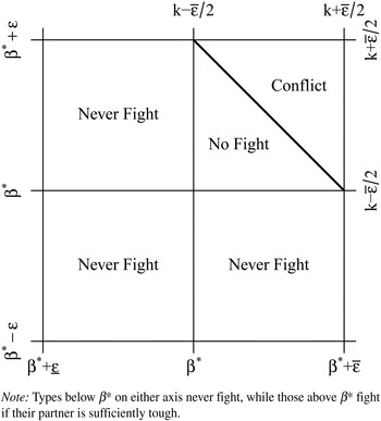
Figure 2 gives a graphical illustration of this point for a noise distribution with bounds
 $[\underline {\varepsilon}, \overline { \varepsilon} ]$
. Each axis spans the toughness distribution for the types, so the square corresponds to all possible pairs of toughness in the stable distribution. When conflict gets extremely costly, the stable preference distribution is always centered on
 $\beta ^{\ast} = k - \overline {\varepsilon} /2$
because this implies the toughest type is
 $\overline \beta = k - \overline {\varepsilon} /2 + \overline { \varepsilon} = k + \overline { \varepsilon} /2$
. So, when β* is matched with the toughest type their aggregate toughness is exactly 2k and a deal is struck.
Illustration of the lower bound on conflict for proposition 1

In the stable preference distribution, anyone who is tougher than average will fight the very toughest types. In particular, the diagonal line in the top-right corner corresponds to the line where β 1 + β 2 = 2k, so for any pair of actors above this line conflict will occur. This corner corresponds to one-eighth of the entire square, illustrating why with a uniform distribution this is the lower bound on the probability of conflict. For non-uniform distributions, there can be more or less density in this corner, but it will never be empty.
The fact that the probability of conflict can remain non trivial even as fighting becomes arbitrarily costly has important implications for the effects of changes in military technology. The most prominent example is the spread of nuclear weapons which affects the possibility and expected costs of interstate war.Footnote 63 Even if nuclear weapons do make war less likely, this effect may be offset by the increased cost of conflict should war occur. As Kydd points out, the most straightforward measure of social welfare is the expected realized cost of war, which is the product of the cost of conflict when it occurs (in our model, k) and the probability it occurs (in our model, Pr(β 1 + β 2 > 2k)).Footnote 64 For example, if the average monetary cost of war between two countries is a billion dollars, and the probability that they fight is 2 percent, then the expected realized cost of war is 20 million dollars. If adding (more) nuclear weapons to the mix increases the cost of war conditional on it occurring to 5 billion dollars but decreases the probability to 1 percent, the expected realized cost would increase to 100 million dollars. However, if the nuclear weapons decrease the probability of war to 0.1 percent, the expected realized cost would decrease to 10 million dollars.
Of course, if nuclear weapons (or other technologies) make war so costly that the probability of occurring is zero, the expected realized costs from war will also be zero. And in our model, when preferences are fixed (as with most bargaining models), the probability of war does become zero if k is sufficiently high as long as there is an upper bound on the toughness.
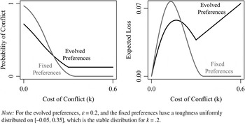
Figure 3 compares the results from a bargaining model with fixed preferences to our model with evolved preferences. The left panel plots the probability of conflict as a function of the cost. The gray curve plots the results with fixed preferences, and the black line plots the probability of conflict from our model (equation 3). As in standard models, the probability of conflict hits zero when fighting becomes sufficiently costly with fixed preferences. However, given the players' evolved preferences in our model, the probability of conflict never goes below 1/8.
Comparison of the probability of conflict and expected loss from conflict in our model and a model with fixed preferences

The right panel shows how this affects the expected realized loss from conflict, which again is the cost of conflict times the probability it occurs: K = kPr(β 1 + β 2 > 2k). With fixed preferences, the expected loss (K) increases for low costs of conflict (because it must be 0 when k = 0), but eventually declines and becomes 0 once the probability of conflict hits 0. On the other hand, with evolved preferences, there is a short range where this expected loss is decreasing in k, but eventually it is always increasing linearly, and hence has no upper bound. This contrast is not limited to the particular example. In fact:
Proposition 2
i) For any fixed toughness distribution, the expected realized loss from conflict K is 0 for sufficiently high k, but
ii) In the stable preference distribution identified by proposition 1, the expected realized loss from conflict approaches infinity as the cost of fighting goes to infinity (i.e., K → ∞ as K → ∞).
Proof
For part (i), let
 $\overline \beta $
be the toughest member of the population. Then if
 $k \gt 2\overline \beta $
, then conflict will never occur. Part (ii) follows immediately from part (ii) of proposition 1.
■
Our results pose a major challenge to the logic of nuclear deterrence. Even if leaders make no mistakes and fully internalize the costs of nuclear war, proposition 1 suggests that no amount of expected destruction can guarantee peace. Perhaps worse, proposition 2 suggests that once the expected costs of war are sufficiently high, further increases to this cost generate no additional deterrent effect, and hence the expected loss from war increases without bound.
Interpreting the result in this fashion requires believing that the evolutionary mechanisms we model apply to leader decision making in the context of potential nuclear war. Of course, nuclear weapons are a recent development in human history, and few have held the responsibility of bargaining in the shadow of nuclear war. Still, as long as evolutionary forces have pushed humans to adopt tougher bargaining stances when the cost of fighting is high, this tendency could project forward to new technologies with a higher level of destruction.
The adjustment to a world where all-out war is extremely costly could occur quite fast through a learning process. For example, former US President Richard Nixon himself recognized the benefit of appearing volatile and belligerent when negotiating with adversarial communist leaders in the shadow of nuclear war, and explained to his White House Chief of Staff, H.R. Haldeman:
I call it the Madman Theory, Bob. I want the North Vietnamese to believe I've reached the point where I might do anything to stop the war. We'll just slip the word to them that, “for God's sake, you know Nixon is obsessed about communism. We can't restrain him when he's angry—and he has his hand on the nuclear button; and Ho Chi Minh himself will be in Paris in two days begging for peace.”Footnote 65
While Nixon suggested seeming willing to start a nuclear war rather than actually being willing to do so, as shown in our formal model, such threats are more credible when actors' preferences actually make them more willing to fight. Furthermore, the presence of just a few truly “crazy” leaders can lead a much larger proportion of “sane” leaders to adopt an aggressive posture similar to the crazy types.Footnote 66
Again, the appendix shows that the central conclusions of proposition 1 and 2 hold for more general evolutionary processes. For example, the result that as the cost of fighting increases the average toughness increases but the probability of conflict decreases holds for a wide class of noise distributions meeting a condition related to having an increasing hazard rate. The fact that conflict must occur in any stable distribution is particularly robust, holding as long as types that attain higher fitness reproduce more often. Finally, the result that the expected realized loss from conflict has no upper bound when k gets arbitrarily large holds as long as the noise in the evolutionary process is bounded. See the appendix for a discussion of the unbounded case (where this property still can hold).
Still, the aim of our analysis is not to make precise predictions about the probability of nuclear war; if it did, the fact that nuclear weapons haven't been used since 1945 would caution against this interpretation. Our main contribution to this debate is to highlight how the assumption that preferences are fixed may be particularly problematic when thinking through the long-term consequences of conflict becoming more costly. Predicting rare events based on past data is difficult for several reasons. The fact that preferences change adds to this challenge, and in our model makes the optimistic projections of deterrence theory look particularly shaky.
Incomplete Information
Even when using a more general evolutionary process, we have made several other consequential assumptions. First, the bargaining protocol is very simple. Still, we expect the result about the inevitability of conflict will generalize: in a proposed world without conflict, there are evolutionary incentives to be more willing to fight since without the realization of conflict there is no drawback to having such preferences. As long as the toughest type is best off in a proposed equilibrium with no conflict, such an equilibrium is impossible.Footnote 67
Second, we allow for preferences to diverge from objective payoffs in only a specific way. In the online supplement we show that our main results hold for a much more general payoff structure where toughness can vary by the role in the bargaining game or preferences over deals can evolve in a flexible manner.
Third, we assume that types are common knowledge, which is particularly problematic given the key role that incomplete information about preferences plays in the literature on bargaining and conflict.Footnote 68 By loosening this assumption, we show that a central conclusion from past work—that incomplete information is a key cause of conflict—can be reversed when preferences are endogenous.Footnote 69 This is because willingness to reject offers can convey an evolutionary advantage only if the proposer knows the responder's taste for fighting. So while making it harder to observe the type of the responder leads to more conflict for fixed preferences, it can also lead the actors to evolve less belligerent preferences, leading to less conflict.
To illustrate this point, we modify the previous model in two ways. First, to keep uncertainty one sided, we assume that players have standard preferences when in the proposer role but that they get subjective payoff v − k + β
r
when fighting in the responder role (see the online supplement for a more detailed discussion of this change). More importantly, we assume that when two players are matched, the type of the responder is observed with probability q. With probability 1–q, the proposer knows only the distribution of toughness in the population. As before, we assume the toughness in a given generation is equal to the toughness of the type that attained the highest fitness in the previous generation plus uniform noise on [−ε
r
, ε
r
], ε
r
> 0. So, responder toughness
 $\beta _m^r $
is stable if given a population distribution uniform on
 $[\beta _m^r - {\varepsilon} ^r, \beta _m^r + {\varepsilon} ^r ]$
, the
 $\beta _m^r $
type attains the highest fitness.
When the type is observed, the analysis is similar to the main model. The type attaining the highest fitness is the toughest which induces an accepted offer. And since the proposer has conflict utility v − k, (i.e., “no toughness”), the responder toughness can be as high as β r = 2k before a higher β r leads to conflict.Footnote 70
When the type is unobserved, the proposer faces a standard risk-reward trade-off where making more generous offers results in reaching more bargains but keeping fewer resources conditional on the offer being accepted. In the range of toughness where a stable preference distribution is possible, the optimal offer has three important properties. First, it is sometimes accepted and sometimes rejected. Second, there are some types who reject this offer but would accept the offer made to them if their type were observed. So, for a fixed preference distribution, the probability of conflict is decreasing in the likelihood that the type is observed. Third, the fitness for accepting the optimal offer made when the type is unobserved is always higher than the conflict payoff.
The type attaining the highest fitness is either the one who gets the best accepted offer when the type is observed (β r = 2k), or the toughest one who accepts the offer when the type is unobserved, which ends up being β r = 2k − ε r . When q is high, the case of observation is more likely, and so the toughness distribution centers on 2k. When q is low, the payoffs from the unobserved case are more important and the toughness distribution is centered on 2k − ε r . For an intermediate range of q neither of these preference distributions is stable, but as shown in the online appendix we can characterize a stable “preference cycle” where the initial generation is centered at 2k, then becomes subsequently less tough for a finite number of generations before “resetting” to 2k.
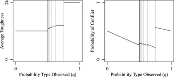
Figure 4 shows how changing the probability of the responder type being observed affects the average toughness and probability of conflict in the stable preference distribution. The vertical lines correspond to points where the stable preference distribution/cycle changes. To the left of the first vertical line and to the right of the last vertical line there is a unique stable preference distribution as we described earlier. In the intermediate interval we plot the average toughness across the stable cycle of toughness across generations.
Average toughness and equilibrium probability of conflict with partially observed preferences

Within any range exhibiting a fixed preference distribution, the probability of conflict is always decreasing in q, in line with standard arguments about how incomplete information fuels conflict.Footnote 71 However, increasing q also leads to jumps up in the average toughness, which lead to jumps up in the probability of conflict. In fact, the highest range of q (i.e., to the right of the last vertical line) exhibits a higher probability of conflict than the lowest range of q (left of the first verticle line) where incomplete information is a major source of conflict but the actors develop less belligerent preferences and never fight when the responder type is observed.
In addition to the abstract contribution to the study of incomplete information and conflict, these results also have implications for how changes in technology affect the likelihood of war. For example, some have argued that international organizations or better intelligence gathering reduce uncertainty about rival states' capabilities or willingness to fight, which can then reduce the possibility of conflict.Footnote 72 If the evolutionary forces described here can act “quickly,” then this model with partially observed preferences provides a counter to this: while making preferences more observable unambiguously leads to more conflict in the short term, it may lead to states or leaders developing even tougher preferences in the long term, which can mitigate or even reverse the short-term effect.
Whether evolution on such a short time scale makes sense depends on the mechanisms of evolution. Biological evolution takes place on a wider time scale which is unlikely to react quickly to shifts in the strategic environment. However, if states learn to elect the kinds of leaders who are successful in the recent past, it may be plausible to conceptualize “generations” as turnover in leadership, which may be quite fast. If changes in the observability of preferences, cost of conflict, or other factors that affect international negotiation change rapidly, it may take only a few generations for citizens to start selecting different kinds of leaders with a more or less warlike disposition.
Conclusion
The idea of a bargaining breakdown leading to conflict plays a particularly important role in the literature on interstate war, but most previous theories do not explicitly model preferences for fighting. Given recent theoretical and empirical insights from behavioral economics and psychology on variation in aggression and propensity to fight, as well as from political science on the importance of leader-specific characteristics influencing crisis behavior, this is an important shortcoming. We provide a theoretical mechanism—evolution of preferences—that bridges these insights with standard political science models of interstate war. More broadly, our results connect with recent research showing how leader socialization influences bargaining and conflict.Footnote 73 Put another way, we demonstrate the importance of environmental context for selecting certain traits (aggressiveness), and how these traits can subsequently influence the bargaining process and likelihood of conflict.
We are agnostic about which type of evolutionary process influences the actors in our model. However, several recent papers suggest that the conflict itself can influence political preferences, with individuals exposed to violence becoming “stuck” in the cycle of violence and less willing to compromise.Footnote 74 Furthermore, other research suggests that exposure to violence changes fundamental preferences, increasing risk, negative reciprocity, and in-group altruism but also fostering cooperation.Footnote 75 Thus, the violence of conflict itself remains an important evolutionary influence, and future work should further explore how preferences shaped by conflict affect bargaining and other political behavior. From a methodological perspective, we have demonstrated that an indirect evolutionary approach is a powerful tool for rigorously modeling how conflict and preferences jointly evolve.
We end on a note of optimism. The idea that game-theoretic models of conflict and psychological models of conflict are diametrically opposed is short sighted. Our approach suggests that these different approaches to explaining conflict are perhaps not as different as they seem. Rather they emphasize different core motivations—for example, emotions and status versus resources and commitment issues—that yield different results. By seeking to incorporate these different motivations in a common framework we provide a new avenue for conflict research and more realistic models of conflict.
Appendix: Formal Definitions and Proofs of Main Results
Single Reproducer Equilibrium Definition
Recall Π(β j ; F, σ) is the expected fitness for a player with toughness β j when matched with a population with toughness distributed according to F and using strategy profile σ. Our main equilibrium definition captures the idea that if the toughness is distributed according to β* + ν where ν follows distribution G, type β* attains the highest fitness when playing the SPNE strategies:
Definiton
A strategy profile
 $\sigma ^{\ast} = (\sigma _1^{\ast}, \sigma _2^{\ast} )$
, reproducing type β*, and noise distribution G(ν) comprise a Single Reproducer Noisy Equilibrium (SRNE) if:
(1)
 $(\sigma _1^{\ast} (\beta _1, \beta _2 ),\sigma _2^{\ast} (\beta _1, \beta _2 ))$
is a SPNE of the bargaining game for all (β
1, β
2) ∈ ℝ2.
(2)
 $\beta ^{\ast} = \arg \mathop {\max} \nolimits_{\beta _j \in {\rm Supp}(G(\nu - \beta ^{\ast} ))} \Pi (\beta _j ;G(\nu - \beta ^{\ast} ),\sigma ^{\ast} )$
The uniform example in the main text is a special case of this definition when G is uniform on [− ε, ε] for ε > 0.
If there is not a unique maximizer of Π, then β* is not well-defined. Conceptually, if there are multiple maximizers, it would be natural to say that all of these types reproduce at an equal rate, or that a randomly chosen type that is among the most fit reproduces. The latter case would at a minimum add substantial complexity to the solution concept because it would require specifying a set of reproducers that all get the exact same payoff. Further, the instability of populations without a unique maximizer is primarily invoked to prevent the case where all types always fight and get the same payoff, and if all types were to reproduce and there is noise in the next generation payoff, the next generation distribution of types will inevitably have a larger support than the previous generation, and hence is not stable. If the reproducer is chosen at random, then the next generation will be stable only if a particular type in the middle happens to be chosen. To avoid formalizing these contingencies, we require that Π have a unique maximizer to have a SRNE.
Derivation of Equation 1, Proof of Lemma 2
Recall β max is continuous and decreasing in β m , with a kink at β m = 2(k − ε). Further, β max has a range [0, ∞) on the defined domain (β m ≤ 2k + ε), ensuring a unique β* such that β max (β*) = β*. If β max (2(k − ε)) < 2(k − ε), this intersection occurs on the first segment of the β max function, which simplifies to:
 $$\displaylines{\beta _{{\rm max}} (2(k - {\varepsilon} )) \lt 2(k - {\varepsilon} ) \cr 2k - (2(k - {\varepsilon} ) + {\varepsilon} ) \lt 2(k - {\varepsilon} ) \cr k \gt \displaystyle{3 \over 2}{\varepsilon}} $$
and when the intersection happens on the first segment, β* is given by:
 $$\displaylines{2k - (\beta ^{\ast} + {\varepsilon} ) = \beta ^{\ast} \cr \beta ^{\ast} = k - \displaystyle{{\varepsilon} \over 2}} $$
When
 $k \lt \displaystyle{3 \over 2}{\varepsilon} $
the intersection happens at the second segment, and β* solves:
 $$\beta ^{\ast} = \displaystyle{{2k - (\beta ^{\ast} - { \varepsilon} )} \over 3}$$
 $$\beta ^{\ast} = \displaystyle{k \over 2} + \displaystyle{{ \varepsilon } \over 4}$$
■
Proof of Proposition 2
Part (i) follows immediately from lemma 2.
For the probability of conflict, the sum of two uniform random variables with the same range follows a triangle distribution. The cumulative density function of β j + β −j is given by:
 $$Pr(\beta _j + \beta _{ - j} \lt x) = \left\{ {\matrix{ {\displaystyle{{(x - 2(\beta ^{\ast} - {\varepsilon} ))^2} \over {8{ \varepsilon} ^2}}} & {x \in [2(\beta ^{\ast} - { \varepsilon} ),2\beta ^{\ast} ]} \cr {1 - \displaystyle{{(2(\beta ^{\ast} + {\varepsilon} ) - x)^2} \over {8{\varepsilon} ^2}}} & {x \in [2\beta ^{\ast}, 2(\beta ^{\ast} + {\varepsilon} )].} \cr}} \right.$$
The equilibrium probability of conflict is 1 − Pr(β
j
+ β
−j
< 2k). The CDF is evaluated on the first segment if and only if 2k < 2β*, or k < β*. When
 $k \le \displaystyle{3 \over 2}{\varepsilon} $
, β* = k/2 + ε/4, so k is less than β* if and only if k < ε/2. When
 $k \gt \displaystyle{3 \over 2}{\rm \varepsilon} $
, β* = k − ε/2 < k, so the CDF is always evaluated on the second segment. Plugging in the appropriate values of β* then gives:
 $$\displaylines{Pr(\beta _j + \beta _{ - j} \gt 2k) = \left\{ {\matrix{ {1 - \displaystyle{{(2k - 2(k/2 + {\varepsilon} /4 - {\varepsilon} ))^2} \over {8{\varepsilon} ^2}}} & {k \le \displaystyle{{\varepsilon} \over 2}} \cr {\displaystyle{{(2(k/2 - { \varepsilon} /4 + { \varepsilon} ) - 2k)^2} \over {8{ \varepsilon} ^2}}} & {k \in \bigg(\displaystyle{{ \varepsilon} \over 2},\displaystyle{3 \over 2}{ \varepsilon} \bigg)} \cr {\displaystyle{{(2(k - { \varepsilon} /2 + { \varepsilon} ) - 2k)^2} \over {8{ \varepsilon} ^2}}} & {k \ge \displaystyle{3 \over 2}{ \varepsilon}} \cr}} \right. \cr \hskip11.4pt = \left\{ {\matrix{ {1 - \displaystyle{{(k + \displaystyle{3 \over 2}{ \varepsilon} )^2} \over {8{ \varepsilon} ^2}}} & {k \le \displaystyle{{ \varepsilon} \over 2}} \cr {\displaystyle{{(k - \displaystyle{5 \over 2}{ \varepsilon} )^2} \over {8{ \varepsilon} ^2}}} & {k \in \bigg(\displaystyle{{ \varepsilon} \over 2},\displaystyle{3 \over 2}{ \varepsilon} \bigg)} \cr {1/8} & {k \ge \displaystyle{3 \over 2}{ \varepsilon}} \cr}} \right.} $$
■
General Unbounded Noise Distributions
Suppose the noise distribution is given by distribution function G with a continuous and differentiable density g.
If the previous generation reproducer was type β m , then the distribution of the current generation types is given by G(β − β m ) with density g(β − β m ). So, the expected fitness for being type β j when β −j is drawn from this distribution can be written:
 $$\Pi (\beta _j ;k,\beta _m ) =\, {\int}_{ - \infty} ^{2k - \beta _j} \left( {v + \displaystyle{{\beta _j - \beta _{ - j}} \over 2}} \right)g(\beta _{ - j} - \beta _m )d\beta _{ - j} + {\int}_{2k - \beta _j} ^\infty \left( {v - k} \right)g(\beta _{ - j} - \beta _m )d\beta _{ - j} $$
We first consider the case where g has full support on ℝ. In this case Π is continuous and differentiable with respect to β j (by the continuity and differentiability of g), and by Lebniz's rule the derivative is:
 $$\eqalign{\displaystyle{{\partial \Pi} \over {\partial \beta _j}} & = g(2k - \beta _j - \beta _m )\left[ {(v - k) - \left( {v + \displaystyle{{\beta _j - (2k - \beta _{ - j} )} \over 2}} \right)} \right]_{\beta _{ - j} = 2k - \beta _j} + \,G(2k - \beta _j - \beta _m )/2 \cr & = - g(2k - \beta _j - \beta _m )\beta _j +G(2k - \beta _j - \beta _m )/2} $$
The first term represents the fact that being slightly tougher results in fighting more types (G(2k − β j − β m )) and the difference between striking a deal and fighting for the marginal type is a loss of v − k − (v − k + β j ) = −β j . The second term represents the better deals achieved when striking a bargain, which is marginal gain of 1/2 times the probability of a deal G(2k − β j − β m ). Setting this derivative to zero and rearranging gives the first-order condition for a maximizer of the fitness function:
 $$\beta _j - \displaystyle{{G(2k - \beta _j - \beta _m )} \over {2g(2k - \beta _j - \beta _m )}} = 0$$
To derive a necessary condition for this equation to have a unique solution, define
 $$dr(\nu ) \equiv \displaystyle{{\partial \displaystyle{{G(\nu )} \over {g(\nu )}}} \over {\partial \nu}} $$
The derivative of the left-hand side of equation (4) with respect to β j is 1 − dr(ν)/2. So, if dr(ν) > −2, then the left-hand side is always increasing. Further, the left-hand side of equation (4) is negative for β j ≤ 0, so dr(ν) > −2 ensures a unique β j maximizing the objective function for each β m .Footnote 76
Since G is increasing, dr(ν) can only be negative where g is increasing. So, for a single-peaked density, dr(ν) is always positive for the ν above the peak, and dr(ν) can only be negative for low values of ν. This condition is related to having an increasing hazard rate, which implies that the inverse hazard rate
 $\displaystyle{{1 - G(\nu )} \over {g(\nu )}}$
is decreasing, that is, dr(ν) − 1/g(ν) is increasing. If further g is symmetric around any ν*, then
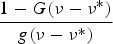 $\displaystyle{{1 - G(\nu - \nu ^{\ast} )} \over {g(\nu - \nu ^{\ast} )}}$
decreasing implies
 $\displaystyle{{1 - G(\nu ^{\ast} - \nu )} \over {g(\nu ^{\ast} - \nu )}} = \displaystyle{{G(\nu - \nu ^{\ast} )} \over {g(\nu - \nu ^{\ast} )}}$
is increasing, that is, dr(ν) > 0. Another standard property which ensures dr(ν) > 0 is if G is log-concave.Footnote
77
For a single peaked density, one way to interpret dr(ν) > − 2 is that the ratio of the distribution to the density of ν does not rapidly increase as ν → −∞, which is also related to the thickness of the left tail of the distribution. Even for a Cauchy distribution, however, dr(ν) is always above –1, which it asymptotically approaches as ν → ∞. For normal distributions dr(ν) is always positive, and for t distributions it is negative for small ν but always above –1.
For multimodal distributions dr(ν) can become very negative at some points, and as a result there can be multiple maxima in this case. To avoid such complications we will assume that dr(ν) is sufficiently positive to guarantee a unique solution to the equilibrium condition.
Since a single-reproducer stable distribution is characterized by a β* such that when β
m
= β* the objective function is maximized at β*, a necessary condition for an β* to be the reproducing type in a SRNE is that
 $\displaystyle{{\partial \Pi} \over {\partial \beta _j}} = 0$
when evaluated at β
j
= β* and β
m
= β*, or:
 $$\eqalign{ - g(2k - 2\beta ^{\ast} )\beta ^{\ast} + G(2k - 2\beta ^{\ast} )/2 = 0 \cr \beta ^{\ast} - \displaystyle{{G(2k - 2\beta ^{\ast} )} \over {2g(2k - 2\beta ^{\ast} )}} = 0} $$
The derivative of the left-hand side with respect to β* is 1 − dr(ν), so as long as dr(ν) > − 1 (which again holds for any normal or t distribution including the Cauchy), there is a unique β* which solves this equation. Further, when setting β m = β*, β j = β* is the global maximizer of Π, and hence the β* solving equation (5) and σ* constitute a SRNE.
Next consider how the stable distribution as changes as k increases. Implicitly differentiating equation (5) gives:
 $$\displaystyle{{\partial \beta ^{\ast}} \over {\partial k}} = - \displaystyle{{ - dr(2k - 2\beta ^{\ast} )} \over {dr(2k - 2\beta ^{\ast} ) + 1}} = \displaystyle{{dr(2k - 2\beta ^{\ast} )} \over {dr(2k - 2\beta ^{\ast} ) + 1}}$$
Since dr(2k − 2β*) > − 1, the denominator is positive, so the sign on this derivative is the same as the sign of dr(2k − 2β*). Further, the derivative is always less than 1 even when it is positive.
The probability of conflict in the stable preference distribution is the probability that two randomly drawn players have toughness greater than 2k. Writing their toughness as β i = β* + ν i , the probability of conflict is:
 $$Pr(\beta ^{\ast} + \nu _1 + \beta ^{\ast} + \nu _2 \gt 2k) = Pr\left( {\displaystyle{{\nu _1 + \nu _2} \over 2} \lt \beta ^{\ast} - k} \right)$$
which since
 $\displaystyle{{\partial \beta ^{\ast}} /{\partial k}} \lt 1$
is decreasing in k.
Summarizing the unbounded noise case:
Proposition 3
For any noise distribution G with density g such that dr(ν) > − 1, there is a unique SRNE. The probability of conflict in the SRNE is decreasing in k. The average toughness in the SRNE is increasing in k if and only if dr(2k − 2β*) > 0.
Proof
See above.
As a final note, recall that dr can only be negative if g is not log-concave, and only for values of ν where g is increasing. So, if g is single peaked around
 $\overline g $
, then whenever
 $k - \beta ^{\ast} \gt \overline g $
the average toughness will be increasing in k. And since
 $\displaystyle{{\partial \beta ^{\ast}} / {\partial k}} \lt 1$
, this must hold for sufficiently large k.
Bounded Noise
Next we consider the case of a general noise distribution with bounds
 $[\underline \nu , \overline \nu ]$
. Again, write the distribution function G and density g. The definition for a SRNE now requires that there exists a β* such that:
 $$\beta ^{\ast} = \mathop {\hbox{arg max}}\limits_{\beta _j \in [\beta ^{\ast} + \underline \nu, \beta ^{\ast} + \overline \nu ]} \Pi (\beta _j ;G(\nu - \beta ^{\ast} ),\sigma ^{\ast} )$$
A necessary condition for a β* meeting this equation is
 $\underline \nu \le 0 \le \overline \nu $
: if not, by definition the maximizing type can't be in the support of the distribution. So, we require that these inequalities hold, and to reduce cases further assume they hold strictly, which implies that some children are weaker and some are tougher than their parents.
Much of the analysis of bounded noise distributions is the same as with unbounded noise albeit with more cases, so we derive only a more general version of the main result from the uniform case: that there is a non-zero lower bound on the probability of conflict.
The fitness payoff for being type β
j
is the same as the unbounded case, though with two important special cases: if
 $\beta _j \lt 2k - (\beta _m + \overline \nu )$
or
 $\beta _j \gt 2k - (\beta _m + \underline \nu )$
the g term drops out. So, the derivative with respect to β
j
is the same as the unbounded case but is undefined at the boundary points (where there is generically a “kink” in the objective function), and equal to 1/2 for low β
j
and 0 for high β
j
:
 $$\eqalign{&\displaystyle{{ \partial \Pi (\beta _j ;G,\beta _m, \sigma ^{\ast} )} \over {\partial \beta _j}} \cr & \qquad \qquad = \left\{ \matrix{ {1/2} \hfill & {\beta _j \lt 2k - (\beta _m + \overline \nu )} \hfill \cr { - g(2k - \beta _j - \beta _m )\beta _j + G(2k - \beta _j - \beta _m )/2} \hfill & {\beta _j \in (2k - (\beta _m + \overline \nu ),2k - (\beta _m + \underline \nu )} \hfill \cr 0 \hfill & \beta _j \gt 2k - (\beta _m + \underline \nu ) \hfill } \right.}$$
Any “interior” solution in the sense that β* lies on the second segment of this function will be characterized by equation (5) as in the unbounded case. However, this solution will not always be interior, as in the uniform case.
More importantly for our result, the fitness function is increasing for any
 $\beta _j \lt 2k - (\beta _m + \overline \nu )$
. So in any stable distribution it must be the case that:
 $$\beta ^{\ast} \ge 2k - (\beta ^{\ast} + \overline \nu ) \Rightarrow \beta ^{\ast} \ge k - \overline \nu /2$$
and so the probability of conflict must be greater than:
 $$Pr(\beta _1 + \beta _2 \ge 2k) \ge Pr(k - \overline \nu /2 + \nu _1 + k - \overline \nu /2 + \nu _2 \ge 2k) = Pr(\nu _1 + \nu _2 \ge \overline \nu )$$
which is equal to 1/8 in the uniform case. More generally:
Proposition 4
For any bounded noise distribution, the probability of conflict in a SRNE is at least:
 $$p_c^{\ast} =\; {\int}_{\nu _1 =\,0}^{\overline \nu} (1 - G(\overline \nu - \nu _1 ))g(\nu _1 )d\nu _1 \gt 0$$
Proof
Follows from writing out the convolution for
 $Pr(\nu _1 + \nu _2 \ge \overline \nu )$
. The expression is greater than zero since
 $\underline \nu \lt 0 \lt \overline \nu $
.■
Visually, this is equivalent to measuring the (density-weighted) area of the top right hand corner of Figure 2 in the main text.
Comparing with the unbounded noise case, the main point of interest is that with unbounded noise the probability of conflict is always decreasing in k (and may approach 0 as K → ∞). while it is always above
 $p_c^{\ast} \gt 0$
when the noise distribution is bounded. So the expected cost of fighting kPr(β
1 + β
2 > 2k) may approach zero as K → ∞ for unbounded noise distributions (though not necessarily; this depends on how quickly the probability of conflict approaches zero). However, for a bounded noise distribution, the expected cost of conflict always approaches infinity as K → ∞.
Multiple Reproducers
Our most general result considers an evolutionary process where more than one type reproduces. Formally, there is a (weakly) positive and increasing “weight function” w:ℝ → ℝ+ which determines how many offspring each player gets as a function of their fitness (where a normalization ensures that the population size is constant). Again, offspring have a toughness equal to their parent's plus a noise term ν drawn from density g with both positive and negative support (i.e., G(0) ∈ (0, 1), where G is the corresponding cumulative density function). So, a distribution of preferences is stable if the density function resulting from this process is equal to the initial density f, or:
 $$f^{\ast} (\beta ) = \;{\int}\, f^{\ast} (\beta - \nu )\displaystyle{{w(\Pi (\beta ;f^{\ast}, \sigma ^{\ast} ))} \over {{\int}\, w(\Pi (\beta ;f^{\ast}, \sigma ^{\ast} ))f^{\ast} (\beta )d\beta}} g(\nu )d\nu $$
Our solution concept for evolution this general process is as follows:
Definition
A density of types f* and strategy profile σ constitute a Multiple Reproducer Noisy Equilibrium (MRNE) if:
(1) σ* is derived from lemma 1.
(2) f* and σ* satisfy equation (7).
While it is difficult to derive conditions when such a stable distribution exists, we can easily show the following:
Proposition 5
For any cost of conflict, weight function, and noise distribution, conflict must occur with positive probability in any MRNE.
Proof
Suppose there was no conflict, and let the highest type in the support of f* be
 $\overline \beta $
(this must be finite, as we have assumed no conflict occurs). For there to be no conflict, it must be the case that
 $\overline \beta \le k$
, and hence Π(β
j
, f*, σ*) is strictly increasing in the support of f*. So, the
 $\overline \beta $
type gets the highest fitness, and hence
 $w(\Pi (\overline \beta ,\ f^{\ast}, \sigma ^{\ast} )) \gt 0$
. (If this were not true,
 ${\int}\, w(\Pi (\beta ;\ f^{\ast}, \sigma ^{\ast} ))f^{\ast} (\beta )d\beta \le \;{\int}\, w(\Pi (\overline \beta ; \ f^{\ast}, \sigma ^{\ast} ))f^{\ast} (\beta )d\beta = 0$
, and hence the right-hand side of equation (7) would be undefined.) Finally, since G(0) ∈ (0, 1), the right-hand side of equation (7) must place positive density on
 $\overline \beta + { \varepsilon} $
for some ε > 0, and by construction
 $f^{\ast}(\overline \beta + { \varepsilon} ) = 0$
, contradicting the equilibrium condition.■
Supplementary Material
Supplementary material for this article is available at <https://doi.org/10.1017/S0020818317000182>.