1 Introduction
Flutter of skin panels is a dangerous phenomenon that can occur in rockets, airplanes and other flight vehicles moving at supersonic speed. These vibrations usually have a high amplitude, cause fatigue damage and decrease skin panel’s lifetime.
First investigations of panel flutter were conducted during WWII, but significant results were obtained in the 1950s–1970s, which are summarised by Bolotin (Reference Bolotin1963), Dowell (Reference Dowell1974) and Novichkov (Reference Novichkov1978).
In most of the panel flutter studies a uniform air flow over a plate was considered, and the boundary layer was neglected. Only a few investigations were devoted to the theoretical (Miles Reference Miles1959; Dowell Reference Dowell1971, Reference Dowell1973; Hashimoto et al. Reference Hashimoto, Aoyama and Nakamura2009; Visbal Reference Visbal2014; Alder Reference Alder2015, Reference Alder2016) and experimental (Muhlstein, Gaspers & Riddle Reference Muhlstein, Gaspers and Riddle1968; Gaspers, Muhlstein & Petroff Reference Gaspers, Muhlstein and Petroff1970) studies of the effect of boundary layer over the plate surface. It is shown that, in the presence of a boundary layer, the flutter can be weakened or completely suppressed. This result was obtained by analysing a particular profile of the boundary layer, which corresponds to a zero-pressure-gradient turbulent boundary layer over a flat plate. However, depending on the flow conditions, qualitatively different boundary layer profiles can be formed over different parts of a flight vehicle.
Gas flow over an elastic plate.

Vedeneev (Reference Vedeneev2013) analytically investigated the influence of an arbitrary boundary layer on the panel flutter in an inviscid shear layer approximation; only long-wave modes were considered. It turned out that its influence on the coupled-mode flutter does not depend on the profile of the boundary layer, whereas for the single-mode flutter its effect is different for generalised convex profiles and profiles with a generalised inflection point. By using numerical calculations, Bondarev & Vedeneev (Reference Bondarev and Vedeneev2016) generalised those results to arbitrary wavelengths.
The first step towards the inclusion of the effect of viscosity into the boundary layer model was done by Bondarev & Vedeneev (Reference Bondarev and Vedeneev2017), who considered viscous boundary layer perturbations at large but finite Reynolds numbers for the case of an infinite plate. It was shown that the effect of the finiteness of the Reynolds number in this case can have both a destabilising and a stabilising effect, depending on the phase speed of the travelling wave. The influence of viscous boundary layer perturbations on panel flutter in the case of finite plates still remains an open question, which is analysed in this study.
The paper is organised as follows. In § 2, we formulate the problem, discuss assumptions and describe the method of solution. Next, in § 3 we derive the pressure perturbation acting on the plate at large but finite Reynolds numbers by using asymptotic Wentzel–Kramers–Brillouin-type solutions. In § 4 we use this expression to close the coupled aeroelastic problem and find the location of its eigenfrequencies on the complex plane by using Kulikovskii’s global instability criterion, and analyse the effect of finite Reynolds numbers. Finally, in § 5 we discuss the results obtained and their possible applications.
2 Formulation of the problem and results of the inviscid analysis
2.1 Formulation of the problem
We consider an elastic plate in a supersonic boundary layer flow of a viscous gas and investigate the influence of the layer on the plate stability (figure 1). It is assumed that the plate represents a skin panel of a flight vehicle, and the local velocity and temperature distributions in the boundary layer are known from the analysis of the steady flow around the vehicle.
The problem is investigated in a two-dimensional (2-D) formulation (all variables do not depend on
 $y$
); also, we neglect the evolution of the boundary layer along the panel length so that the unperturbed flow does not depend on
 $x$
. This assumption is valid if the plate length
 $L$
is small enough in comparison with the distance at which the boundary layer is essentially changed. All variables are assumed to be non-dimensional, with the speed of sound
 $a_{\infty }$
and temperature of the flow
 $T_{\infty }$
taken as the velocity and temperature scales (the subscript ‘
 $\infty$
’ denotes dimensional parameters of the flow outside the boundary layer), the plate thickness
 $h$
as the length scale and plate material density as the density scale. The Reynolds number is defined as
 $R=u_{\infty }\tilde{\unicode[STIX]{x1D6FF}}/\unicode[STIX]{x1D708}_{\infty }$
, where
 $u_{\infty }$
and
 $\unicode[STIX]{x1D708}_{\infty }$
are the flow speed and the kinematic viscosity,
 $\tilde{\unicode[STIX]{x1D6FF}}$
is the dimensional thickness of the boundary layer.
The motion of the plate is described by the Kirchhoff–Love small deflection plate theory. In a dimensionless form, the plate equation is as follows:
 $$\begin{eqnarray}D\frac{\unicode[STIX]{x2202}^{4}w}{\unicode[STIX]{x2202}x^{4}}-M_{w}^{2}\frac{\unicode[STIX]{x2202}^{2}w}{\unicode[STIX]{x2202}x^{2}}+\frac{\unicode[STIX]{x2202}^{2}w}{\unicode[STIX]{x2202}t^{2}}+p(x,0,t)=0,\end{eqnarray}$$
where
 $w(x,t)$
is the plate deflection,
 $D$
is its stiffness,
 $M_{w}$
is the square root of the dimensionless in-plane tension force and
 $p(x,z,t)$
is the flow pressure disturbance induced by the plate motion, such that
 $p$
is a function of
 $w$
.
Two boundary conditions must be specified at each plate edge. For example, these could be clamping, pinning or free-edge boundary conditions.
To simplify the study we assume that the boundary layer, with given undisturbed velocity and temperature profiles, is laminar up to high Reynolds numbers. This assumption can be justified by the fact that laminar boundary layers are observed in experiments up to
 $R\sim 10^{5}$
for the Reynolds number based on the boundary layer thickness (Gaponov & Maslov Reference Gaponov and Maslov1980). For turbulent boundary layers this simplification can be used as the first approximation if the dominant turbulent fluctuation frequencies are much higher than the frequency of the growing plate oscillations.
The perturbations of a perfect viscous gas with a boundary layer-type mean flow are described by the linearised Navier–Stokes equations (Lees & Lin Reference Lees and Lin1946). The boundary conditions for the perturbations are as follows:
(i) the no-slip and adiabatic conditions along the moving plate surface;
(ii) radiation condition as
 $z\rightarrow \infty$
.

Note that the adiabaticity of perturbations does not imply heat insulation for the mean flow.
Hence, the plate and the gas motions are coupled in both ways: first, the plate moves under the action of the flow pressure (2.1); second, the flow is perturbed by the plate through the no-slip boundary condition, i.e. the normal (vertical) flow speed should be equal to the plate speed, and the tangential (horizontal) flow speed should be zero.
We will assume than the plate length is large in terms of the Kulikovskii (Reference Kulikovskii1966) instability condition. He proved that the stability criterion for systems of large finite length is generally different from the criterion for an infinite system, but the analysis of a finite length system can be reduced to the study of infinite system waves. Vedeneev (Reference Vedeneev2012, Reference Vedeneev2016) showed that for the 2-D panel flutter problem, the Kulikovskii criterion yields reliable predictions of the flutter boundary for the panel parameters actually used in aviation. Before proceeding to the study of the problem, let us briefly describe the Kulikovskii global instability criterion.
2.2 The global instability criterion
Kulikovskii (Reference Kulikovskii1966) proved that there are two instability types of a system of large but finite length: the ‘one-side’ and ‘global’ instabilities. Accordingly, the growing perturbations can have the form of either one-side eigenfunctions, which are determined by the reflection of waves from one boundary, or global eigenfunctions, representing two waves travelling in opposite directions, turning into each other when reflected from the boundaries of the system.
The typical boundary conditions for the plate (clamped, pinned or free edge) do not satisfy the condition of the one-side instability of 2-D perturbations (Vedeneev Reference Vedeneev2005). Thus, the flutter can occur only in the form of the global instability.
To describe the global instability criterion, let us number the spatial roots
 $k_{j}(\unicode[STIX]{x1D714})$
of the dispersion equation for an infinite system in the order of decrease of
 $\text{Im}\,k_{j}(\unicode[STIX]{x1D714})$
as
 $\text{Im}\,\unicode[STIX]{x1D714}\rightarrow +\infty$
:
 $$\begin{eqnarray}\text{Im}\,k_{1}>\cdots >\text{Im}\,k_{s}>0>\text{Im}\,k_{s+1}>\cdots >\text{Im}\,k_{N},\end{eqnarray}$$
where
 $\unicode[STIX]{x1D714}$
is a complex frequency. Next, we split the roots into two groups: the first is such that
 $\text{Im}\,k_{j}(\unicode[STIX]{x1D714})>0$
,
 $j=1,\ldots ,s$
; the second is such that
 $\text{Im}\,k_{j}(\unicode[STIX]{x1D714})<0$
,
 $j=s+1,\ldots ,N$
as
 $\text{Im}\,\unicode[STIX]{x1D714}\rightarrow +\infty$
. The first and second groups represent the waves travelling in the positive and negative
 $x$
directions, respectively.
According to global instability criterion, as the length of the system
 $L\rightarrow \infty$
, its eigenfrequencies tend to the curve
 $\unicode[STIX]{x1D6FA}$
in the
 $\unicode[STIX]{x1D714}$
-plane defined by the following equation:
 $$\begin{eqnarray}\min _{1\leqslant p\leqslant s}\text{Im}\,k_{p}(\unicode[STIX]{x1D714})=\max _{s+1\leqslant q\leqslant N}\text{Im}\,k_{q}(\unicode[STIX]{x1D714}).\end{eqnarray}$$
Thus, the instability criterion of long finite systems is as follows: the system is unstable if a piece of the
 $\unicode[STIX]{x1D6FA}$
curve is located in the
 $\text{Im}\,\unicode[STIX]{x1D714}>0$
half-plane.
For an infinite plate in a gas flow, by considering the travelling-wave solution
 $w(x,t)=\text{e}^{\text{i}(kx-\unicode[STIX]{x1D714}t)}$
,
 $p(x,z,t)=\unicode[STIX]{x03C0}(z)\text{e}^{\text{i}(kx-\unicode[STIX]{x1D714}t)}$
, the dispersion equation
 ${\mathcal{D}}(k,\unicode[STIX]{x1D714})=0$
is readily obtained from (2.1):
 $$\begin{eqnarray}{\mathcal{D}}(k,\unicode[STIX]{x1D714})=Dk^{4}+M_{w}^{2}k^{2}-\unicode[STIX]{x1D714}^{2}+\unicode[STIX]{x03C0}(0)=0.\end{eqnarray}$$
Spatial roots
 $k_{1}$
and
 $k_{2}$
correspond to the waves travelling downstream, and
 $k_{3}$
and
 $k_{4}$
correspond to the waves travelling upstream (Vedeneev Reference Vedeneev2013), where
 $\text{Im}\,k_{1}>\text{Im}\,k_{2}>0>\text{Im}\,k_{3}>\text{Im}\,k_{4}$
as
 $\text{Im}\,\unicode[STIX]{x1D714}\rightarrow +\infty$
. According to the Kulikovskii criterion, as the length of the plate
 $L\rightarrow \infty$
, its eigenfrequencies in a gas flow tend to the curve
 $\unicode[STIX]{x1D6FA}$
in the
 $\unicode[STIX]{x1D714}$
-plane defined by the following equation:
 $$\begin{eqnarray}\text{Im}\,k_{2}(\unicode[STIX]{x1D714})=\text{Im}\,k_{3}(\unicode[STIX]{x1D714}),\end{eqnarray}$$
which corresponds to the single-mode flutter of the plate (Vedeneev Reference Vedeneev2005, Reference Vedeneev2012, Reference Vedeneev2013). Eigenfrequencies corresponding to the other type of panel flutter, coupled-mode flutter, tend to the curve
 $$\begin{eqnarray}\text{Im}\,k_{2}(\unicode[STIX]{x1D714})=\text{Im}\,k_{4}(\unicode[STIX]{x1D714}),\end{eqnarray}$$
but they are not considered in this study, because the boundary layer effect on this flutter type is minor (Vedeneev Reference Vedeneev2013).
Let us now briefly review the results of our previous studies devoted to the inviscid-flow problem.
2.3 Inviscid approximation
Vedeneev (Reference Vedeneev2013) and Bondarev & Vedeneev (Reference Bondarev and Vedeneev2016) studied the problem under consideration for the Reynolds number
 $R=\infty$
, i.e. in the inviscid approximation. Comparison of the asymptotic results obtained through the Kulikovskii criterion for plates in uniform flow with solutions of the full eigenvalue problem (Vedeneev Reference Vedeneev2012, Reference Vedeneev2016) shows that the results are reliable for dimensionless plate lengths (i.e. plate length rated to the plate thickness)
 $L\gtrsim 100$
. It is expected that results obtained for the boundary layer flow are valid for the same plate lengths.
Let us call the boundary layer profile with
 $$\begin{eqnarray}\frac{\text{d}}{\text{d}z}\left(\frac{1}{T}\frac{\text{d}u}{\text{d}z}\right)<0\end{eqnarray}$$
for
 $z\in [0;\unicode[STIX]{x1D6FF})$
the generalised convex profile (Lees & Lin Reference Lees and Lin1946), where
 $u,T$
are the velocity and temperature profiles of the undisturbed flow,
 $\unicode[STIX]{x1D6FF}$
is the thickness of the boundary layer. Accelerating supersonic flows, which usually occur along convex walls, are examples of generalised convex boundary layer profiles. For this type of boundary layer it has been proven that an increase of the layer thickness yields an increase of the frequencies of growing eigenmodes and a decrease of their growth rates. For sufficiently thick boundary layers the plate is fully stabilised. These conclusions are in agreement with the stabilisation of the plate by the zero-pressure-gradient boundary layer observed in the experimental and theoretical studies of Muhlstein et al. (Reference Muhlstein, Gaspers and Riddle1968), Gaspers et al. (Reference Gaspers, Muhlstein and Petroff1970), Dowell (Reference Dowell1973), Hashimoto et al. (Reference Hashimoto, Aoyama and Nakamura2009) and Alder (Reference Alder2015, Reference Alder2016).
The case of the boundary layer profile with a generalised inflection point
 $z_{i}$
, where
 $(u^{\prime }/T)^{\prime }=0$
, was also considered (the prime denotes differentiation with respect to
 $z$
). In subsonic flow, such a profile would be unstable, because the existence of the generalised inflection point is a necessary and sufficient condition for the inviscid instability of subsonic disturbances (Lees & Lin Reference Lees and Lin1946). However, in supersonic flow, there exist such profiles (for example, in flows over certain concave walls) such that the generalised inflection point is located in the supersonic (with respect to the mean flow) part of the boundary layer, i.e.
 $u(z_{i})<M-1,$
where
 $M=u_{\infty }/a_{\infty }$
is the Mach number. Vedeneev (Reference Vedeneev2013) showed that such a profile can be stable and therefore can exist in real flows. We proved that, for this type of boundary layer, the thickening of the layer first yields the increase of the growth rates accompanied by the widening of the frequency range of growing eigenmodes. For higher thicknesses, growth rates decrease and tend towards 0 as
 $\unicode[STIX]{x1D6FF}\rightarrow \infty$
; however, they stay positive. As a result the boundary layer can have an essentially destabilising effect.
In this study we will investigate the effect of viscosity on single-mode flutter. However, prior to considering the coupled aeroelastic problem, in the next section we will study perturbations of the boundary layer induced by the wall motion.
3 Viscous perturbations of the boundary layer
Hereafter, the Reynolds number is assumed to be large but finite.
3.1 System of equations for perturbations
Let us consider linearised dimensionless travelling-wave perturbations of the flow (Lees & Lin Reference Lees and Lin1946) expressed by the following functions:
 $$\begin{eqnarray}z_{1}=f;\quad z_{2}=f^{\prime };\quad z_{3}=\unicode[STIX]{x1D711};\quad z_{4}={\displaystyle \frac{\unicode[STIX]{x03C0}}{M^{2}}};\quad z_{5}=\unicode[STIX]{x1D703};\quad z_{6}=\unicode[STIX]{x1D703}^{\prime }.\end{eqnarray}$$
Here,
 $f$
,
 $\unicode[STIX]{x1D703}$
are the non-dimensional perturbation amplitudes of the horizontal velocity component (
 $x$
-component) and temperature. Lees & Lin (Reference Lees and Lin1946) used different scales in the non-dimensionalisation, which we will retain in this section. Namely, the velocity and the temperature outside of the boundary layer are chosen as velocity and temperature scales, respectively. The thickness of the boundary layer is taken as the length scale. The function
 $\unicode[STIX]{x1D711}$
characterises the non-dimensional perturbation of the vertical component of velocity, which is related as
 $v_{z}=k\unicode[STIX]{x1D711}(z)\text{e}^{\text{i}(kx-\unicode[STIX]{x1D714}t)}$
. The function
 $\unicode[STIX]{x03C0}$
is the non-dimensional pressure perturbation, with
 $\unicode[STIX]{x1D70C}_{\infty }u_{\infty }^{2}/(\unicode[STIX]{x1D6FE}M^{2})$
taken as the pressure scale, where
 $\unicode[STIX]{x1D6FE}$
is the adiabatic index.
According to the boundary layer theory, we will assume a steady pressure
 $P(z)=\text{const}.$
Also, the perturbation of the dynamic viscosity is related to the temperature perturbation as follows:
 $m=\unicode[STIX]{x1D703}(\text{d}\unicode[STIX]{x1D707}_{dyn}/\text{d}T)$
, where
 $\unicode[STIX]{x1D707}_{dyn}$
is the non-dimensional dynamic viscosity, with its value in the mean flow taken as the characteristic scale. Below, for simplicity, it is assumed that the dynamic viscosity is constant and
 $m=0$
(much longer algebra shows that without this simplification the results are the same as those presented below). Then the linearised dimensionless system of equations for gas perturbations takes the form (Lees & Lin Reference Lees and Lin1946)
 $$\begin{eqnarray}\left.\begin{array}{@{}c@{}}z_{1}^{\prime }=z_{2},\\ z_{2}^{\prime }={\displaystyle \frac{kR}{\displaystyle \unicode[STIX]{x1D708}\unicode[STIX]{x1D70C}}}\left(\unicode[STIX]{x1D70C}(\text{i}(u-c)z_{1}+u^{\prime }z_{3})+{\displaystyle \frac{\displaystyle \text{i}}{\displaystyle \unicode[STIX]{x1D6FE}}}z_{4}\right)+O(1),\\ z_{3}^{\prime }=-\text{i}z_{1}-{\displaystyle \frac{\displaystyle \unicode[STIX]{x1D70C}^{\prime }}{\displaystyle \unicode[STIX]{x1D70C}}}z_{3}-\text{i}(u-c)\left({\displaystyle \frac{z_{4}M^{2}}{p}}-{\displaystyle \frac{z_{5}}{T}}\right),\\ z_{4}^{\prime }=\left(1+{\displaystyle \frac{1}{R}}O(1)\right)^{-1}\times \left(-\unicode[STIX]{x1D6FE}k^{2}\unicode[STIX]{x1D70C}\text{i}(u-c)z_{3}+{\displaystyle \frac{1}{R}}O(1)\right),\\ z_{5}^{\prime }=z_{6},\\ z_{6}^{\prime }={\displaystyle \frac{kRPr}{\unicode[STIX]{x1D6FE}\unicode[STIX]{x1D708}\unicode[STIX]{x1D70C}}}\left(\unicode[STIX]{x1D6FE}\unicode[STIX]{x1D70C}(T^{\prime }z_{3}+\text{i}(u-c)z_{5})-\text{i}(\unicode[STIX]{x1D6FE}-1)(u-c)z_{4}M^{2}\right)\\ -\,2Pr(\unicode[STIX]{x1D6FE}-1)M^{2}u^{\prime }(z_{2}+\text{i}k^{2}z_{3})+k^{2}z_{5},\end{array}\right\}\end{eqnarray}$$
where
 $c=\unicode[STIX]{x1D714}/k$
is a phase speed;
 $\unicode[STIX]{x1D70C}$
and
 $\unicode[STIX]{x1D708}$
are the non-dimensional density and kinematic viscosity of the undisturbed flow, with
 $\unicode[STIX]{x1D70C}_{\infty }$
and
 $\unicode[STIX]{x1D708}_{\infty }$
taken as characteristic scales, respectively;
 $Pr$
is the Prandtl number, and
 $O(1)$
are functions of
 $z_{j}$
, which have the order of unity as
 $R\rightarrow \infty$
.
The general solution of the system (3.2) consists of a combination of six linearly independent solutions. In the case of
 $R\rightarrow \infty$
these solutions can be approximated by two regular solutions, transforming into the solutions of the Rayleigh equation as
 $R\rightarrow \infty$
, and four solutions of WKB (Wentzel–Kramers–Brillouin) type, having the asymptotic form
 $z_{i}(z)=f_{i}(z)\exp (g_{0}(z)\sqrt{kR})$
(Lees & Lin Reference Lees and Lin1946).
3.2 Regular solutions
In the case of inviscid approximation (
 $R=\infty$
) we can derive from (3.2) an ordinary second-order differential equation for the vertical component of the velocity perturbation, known as the compressible Rayleigh equation (Lees & Lin Reference Lees and Lin1946):
 $$\begin{eqnarray}\frac{\text{d}}{\text{d}z}\left(\frac{(u-c)\unicode[STIX]{x1D711}^{\prime }-u^{\prime }\unicode[STIX]{x1D711}}{T-M^{2}(u-c)^{2}}\right)-\frac{k^{2}}{T}(u-c)\unicode[STIX]{x1D711}=0.\end{eqnarray}$$
The pressure perturbation is expressed in terms of the perturbation of the vertical velocity component as
 $$\begin{eqnarray}\unicode[STIX]{x03C0}=-\text{i}\unicode[STIX]{x1D6FE}M^{2}\left({\displaystyle \frac{(u-c)\unicode[STIX]{x1D711}^{\prime }-u^{\prime }\unicode[STIX]{x1D711}}{T-M^{2}(u-c)^{2}}}\right).\end{eqnarray}$$
The Rayleigh equation can have two singularities (Lees & Lin Reference Lees and Lin1946). The first one is the point
 $z$
, where
 $T(z)-M^{2}(u(z)-c)^{2}=0$
; this singularity is removable. The other one is the critical point
 $z_{c}$
, where
 $u(z_{c})=c$
; it leads to the logarithmic singularity of the solution.
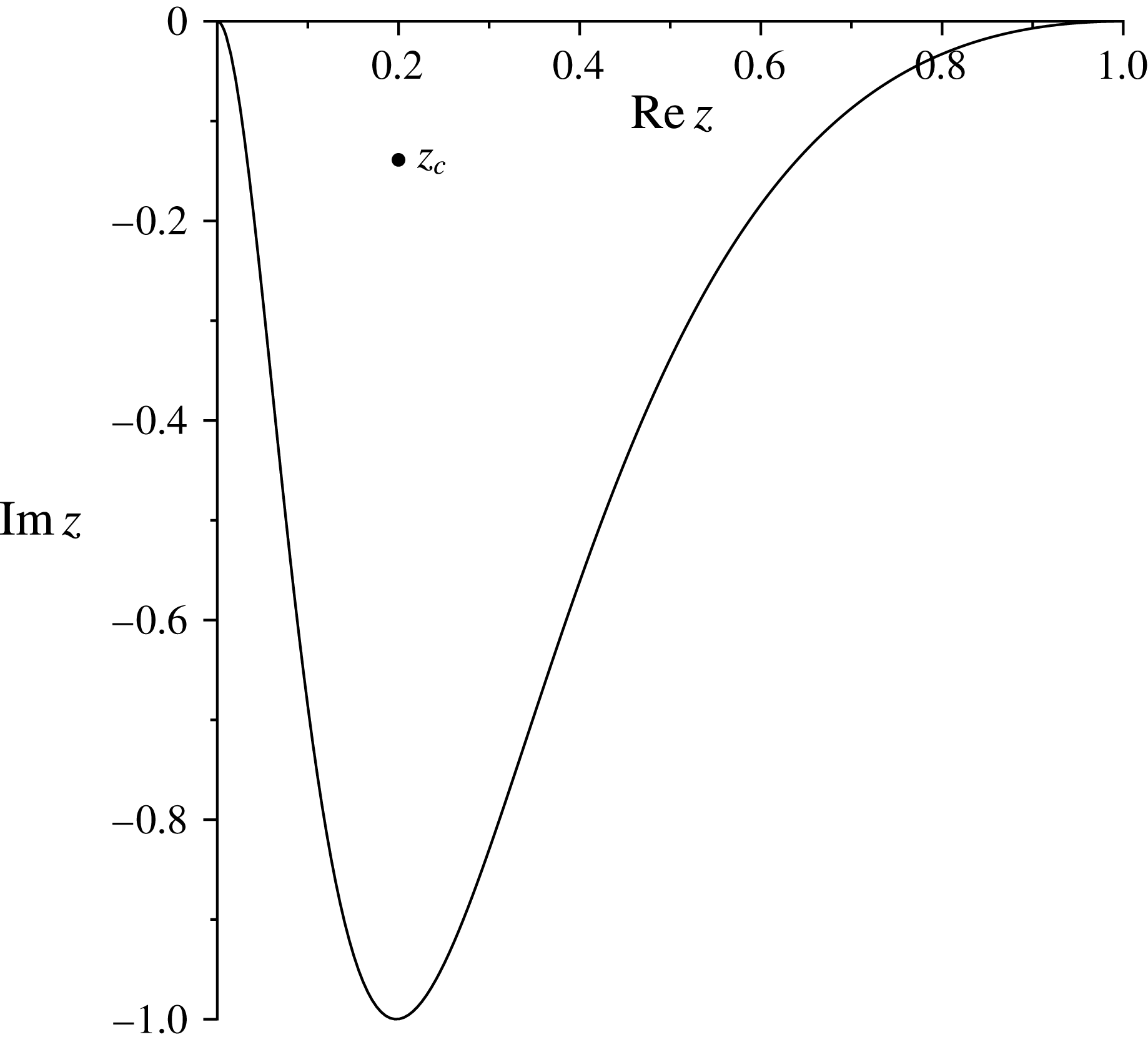
Integration path chosen for solving the Rayleigh equation for the velocity profile
 $u(\unicode[STIX]{x1D702})=M\sin (\unicode[STIX]{x03C0}\unicode[STIX]{x1D702}/2)$
,
 $M=1.6$
,
 $c=0.5-0.33\text{i}$
. The critical point is
 $z_{c}\approx 0.20-0.14\text{i}$
,
 $\unicode[STIX]{x1D6FF}=1$
.

In order to obtain a solution that is a limit of the viscous solution as
 $R\rightarrow \infty$
the critical point must be passed below in the complex
 $z$
-plane (Drazin & Reid Reference Drazin and Reid2004; Lees & Lin Reference Lees and Lin1946) (figure 2). Consequently, to solve the Rayleigh equation, the integration from
 $z=0$
to
 $z=1$
must be carried out along a smooth curve passing below the critical point. In particular, in the case of growing perturbations,
 $\text{Im}(z_{c})>0$
, the integration can be carried out along the real axis
 $z$
in the complex
 $z$
-plane, but this is not the case for neutral and damped perturbations,
 $\text{Im}(z_{c})\leqslant 0$
.
Consider boundary conditions for the Rayleigh equation. First, at the plate surface
 $z=0$
, we assign the condition of impenetrability along the oscillating plate. The second condition is placed on the boundary layer edge
 $z=1$
. Since the flow is homogeneous for
 $z>1$
, the Rayleigh equation (3.3) reduces to an equation with constant coefficients and has the solution
 $v(z)=C\text{e}^{-\unicode[STIX]{x1D6FD}z}$
,
 $\unicode[STIX]{x1D6FD}=k\sqrt{1-M^{2}(1-c)^{2}}$
. The radiation condition as
 $z\rightarrow +\infty$
yields a particular square root branch, namely,
 $\text{Re}\,\unicode[STIX]{x1D6FD}>0$
as
 $\text{Im}\,\unicode[STIX]{x1D714}\rightarrow +\infty$
. This exponentially decaying solution outside the boundary layer must be matched with the solution inside the boundary layer, which yields the second boundary condition. Thus, the boundary conditions take the following form:
 $$\begin{eqnarray}\unicode[STIX]{x1D711}=-\text{i}c\quad (z=0),\quad \frac{\text{d}\unicode[STIX]{x1D711}}{\text{d}z}+\unicode[STIX]{x1D6FD}\unicode[STIX]{x1D711}=0\quad (z=1).\end{eqnarray}$$
3.3 WKB solutions
These solutions can be represented by the following expansions in series of the small parameter
 $\unicode[STIX]{x1D700}=1/\sqrt{kR}$
 $$\begin{eqnarray}z_{i}=(B_{i0}(z)+B_{i1}(z)\unicode[STIX]{x1D700}+B_{i2}(z)\unicode[STIX]{x1D700}^{2}+\cdots \,)\exp \left(\frac{g_{0}(z)}{\unicode[STIX]{x1D700}}\right).\end{eqnarray}$$
Two types of WKB solutions are obtained by substituting
 $z_{i}$
into the system of equations (3.2) (Lees & Lin Reference Lees and Lin1946). The first type has the form
 $$\begin{eqnarray}\left.\begin{array}{@{}c@{}}B_{10}=\text{const.}_{1}(u-c)^{-3/4}\left(\frac{\displaystyle \text{i}}{\displaystyle \unicode[STIX]{x1D708}}\right)^{-1/4},\\ B_{30}=B_{40}=B_{50}=0,\\ B_{31}=-\text{i}\,\text{const.}_{1}(u-c)^{-5/4}\left(\frac{\displaystyle \text{i}}{\displaystyle \unicode[STIX]{x1D708}}\right)^{-3/4},\\ B_{41}=0,\\ g_{0}=\displaystyle \int _{z^{\ast }}^{z}\sqrt{\frac{\displaystyle \text{i}}{\displaystyle \unicode[STIX]{x1D708}}(u-c)}\,\text{d}z,\end{array}\right\}\end{eqnarray}$$
which is called the viscous solution. The second one has the form
 $$\begin{eqnarray}\left.\begin{array}{@{}c@{}}B_{10}=B_{30}=B_{40}=0,\\ B_{41}=0,\\ B_{50}=\text{const.}_{2}T^{1/2}(u-c)^{-1/4}\left(\frac{\displaystyle \text{i}Pr}{\displaystyle \unicode[STIX]{x1D708}}\right)^{1/2},\\ g_{0}=\displaystyle \int _{z^{\ast }}^{z}\sqrt{\frac{\displaystyle \text{i}Pr}{\displaystyle \unicode[STIX]{x1D708}}(u-c)}\,\text{d}z,\end{array}\right\}\end{eqnarray}$$
which is called the temperature solution.
Both viscous and temperature solutions contain a pair of solutions, differing in the choice of the root branch in
 $g_{0}$
.
3.4 Pressure disturbance
Thus, the general solution of the system (3.2) consists of two regular solutions, two viscous solutions and two temperature solutions (Lees & Lin Reference Lees and Lin1946). We have to choose a certain branch of the roots in
 $g_{0}$
in the viscous and temperature solutions to satisfy the radiation condition at infinity (as the other branches correspond to exponentially growing solutions as
 $z\rightarrow +\infty$
). Hence, a single solution of each type remains of the two viscous and two temperature solutions. From two linearly independent regular solutions, one linear combination can be formed to satisfy the radiation condition at infinity. Thus, the solution of the system of (3.2), which satisfies the radiation condition, is now a combination of only three linearly independent solutions (regular, viscous and temperature)
 $$\begin{eqnarray}\left.\begin{array}{@{}c@{}}f(z)=c_{1}\,f_{r}(z)+c_{2}\,f_{v}(z)+c_{3}\,f_{t}(z),\\ \unicode[STIX]{x1D711}(z)=c_{1}\unicode[STIX]{x1D711}_{r}(z)+c_{2}\unicode[STIX]{x1D711}_{v}(z)+c_{3}\unicode[STIX]{x1D711}_{t}(z),\\ \unicode[STIX]{x1D703}(z)=c_{1}\unicode[STIX]{x1D703}_{r}(z)+c_{2}\unicode[STIX]{x1D703}_{v}(z)+c_{3}\unicode[STIX]{x1D703}_{t}(z),\end{array}\right\}\end{eqnarray}$$
as well as
 $$\begin{eqnarray}\unicode[STIX]{x03C0}(z)=c_{1}\unicode[STIX]{x03C0}_{r}(z)+c_{2}\unicode[STIX]{x03C0}_{v}(z)+c_{3}\unicode[STIX]{x03C0}_{t}(z),\end{eqnarray}$$
where the indexes
 $r$
,
 $v$
,
 $t$
denote regular, viscous and temperature solutions, respectively.
These solutions can be represented by the following expansions in series of the small parameter
 $\unicode[STIX]{x1D700}$
 $$\begin{eqnarray}\left.\begin{array}{@{}c@{}}f_{r}=f_{inv}\,+\,f_{r}^{2}\unicode[STIX]{x1D700}^{2}+\cdots \,;\\ f_{v,t}=(f_{v,t}^{0}+f_{v,t}^{1}\unicode[STIX]{x1D700}+f_{v,t}^{2}\unicode[STIX]{x1D700}^{2}+\cdots \,)\exp \left({\displaystyle \frac{\displaystyle g_{0(v,t)}}{\unicode[STIX]{x1D700}}}\right),\end{array}\right\}\end{eqnarray}$$
where index ‘inv’ denotes the inviscid solution (i.e. the solution of the Rayleigh equation). Similar expansions hold for
 $\unicode[STIX]{x1D711},\unicode[STIX]{x1D703}$
and
 $\unicode[STIX]{x03C0}$
.
Expressions (3.7) and (3.8) show that
 $B_{40}=B_{41}=0$
for both viscous and temperature solutions, i.e.
 $\unicode[STIX]{x03C0}_{v}(z)=O(\unicode[STIX]{x1D700}^{2})$
and
 $\unicode[STIX]{x03C0}_{t}(z)=O(\unicode[STIX]{x1D700}^{2})$
. Since
 $\unicode[STIX]{x03C0}_{r}$
is a regular solution of the system (3.2), then
 $$\begin{eqnarray}\unicode[STIX]{x03C0}_{r}(z)=\unicode[STIX]{x03C0}_{inv}(z)+O(\unicode[STIX]{x1D700}^{2}).\end{eqnarray}$$
We obtain that the pressure perturbation
 $\unicode[STIX]{x03C0}(z)$
(3.10) can be written as
 $$\begin{eqnarray}\unicode[STIX]{x03C0}(z)=c_{1}(\unicode[STIX]{x1D700})\unicode[STIX]{x03C0}_{inv}(z)+O(\unicode[STIX]{x1D700}^{2}).\end{eqnarray}$$
Therefore, to find the first approximation for the pressure perturbation, we need to calculate
 $c_{1}(\unicode[STIX]{x1D700})$
, since only it has a linear term in the expansion in
 $\unicode[STIX]{x1D700}$
(3.13).
To calculate
 $c_{1}(\unicode[STIX]{x1D700})$
, we consider the no-slip condition on the plate surface and assume that the plate is adiabatic with respect to the perturbations (which, however, does not imply heat insulation for the mean flow):
 $$\begin{eqnarray}\left.\begin{array}{@{}c@{}}z_{1}=f=0,\\ z_{3}=\unicode[STIX]{x1D711}=-\text{i}c,\\ z_{6}=\unicode[STIX]{x1D703}^{\prime }=0.\end{array}\right\}\end{eqnarray}$$
Substitute (3.9) into the boundary conditions to obtain
 $$\begin{eqnarray}\left.\begin{array}{@{}c@{}}c_{1}\,f_{r}(0)+c_{2}\,f_{v}(0)+c_{3}\,f_{t}(0)=0,\\ c_{1}\unicode[STIX]{x1D711}_{r}(0)+c_{2}\unicode[STIX]{x1D711}_{v}(0)+c_{3}\unicode[STIX]{x1D711}_{t}(0)=-\text{i}c,\\ c_{1}\unicode[STIX]{x1D703}_{r}^{\prime }(0)+c_{2}\unicode[STIX]{x1D703}_{v}^{\prime }(0)+c_{3}\unicode[STIX]{x1D703}_{t}^{\prime }(0)=0.\end{array}\right\}\end{eqnarray}$$
Using Cramer’s rule, we calculate
 $c_{1}=\unicode[STIX]{x1D6E5}_{1}/\unicode[STIX]{x1D6E5},$
where
 $$\begin{eqnarray}\unicode[STIX]{x1D6E5}_{1}=\left|\begin{array}{@{}ccc@{}}0 & f_{v} & f_{t}\\ -\text{i}c & \unicode[STIX]{x1D711}_{v} & \unicode[STIX]{x1D711}_{t}\\ 0 & \unicode[STIX]{x1D703}_{v}^{\prime } & \unicode[STIX]{x1D703}_{t}^{\prime }\end{array}\right|,\quad \unicode[STIX]{x1D6E5}=\left|\begin{array}{@{}ccc@{}}f_{r} & f_{v} & f_{t}\\ \unicode[STIX]{x1D711}_{r} & \unicode[STIX]{x1D711}_{v} & \unicode[STIX]{x1D711}_{t}\\ \unicode[STIX]{x1D703}_{r}^{\prime } & \unicode[STIX]{x1D703}_{v}^{\prime } & \unicode[STIX]{x1D703}_{t}^{\prime }\end{array}\right|,\end{eqnarray}$$
and values of the functions are taken at
 $z=0$
. Next, the velocity and temperature perturbations in the form of expansions (3.11) should be substituted here. Taking into account
 $g_{0}$
for the viscous and temperature cases (3.7), (3.8), we obtain:
 $$\begin{eqnarray}c_{1}(\unicode[STIX]{x1D700})={\displaystyle \frac{-\text{i}c}{\unicode[STIX]{x1D711}_{inv}}}+{\displaystyle \frac{-\text{i}c}{\unicode[STIX]{x1D711}_{inv}}}\left({\displaystyle \frac{f_{inv}}{\unicode[STIX]{x1D711}_{inv}}}{\displaystyle \frac{\unicode[STIX]{x1D711}_{v}^{1}}{f_{v}^{0}}}\right)\unicode[STIX]{x1D700}+O(\unicode[STIX]{x1D700}^{2}).\end{eqnarray}$$
Using the system of equations for the inviscid approximation (Lees & Lin Reference Lees and Lin1946) and the expressions for
 $\unicode[STIX]{x1D711}_{v}^{1}$
,
 $f_{v}^{0}$
from the § 3.3 (
 $B_{31}$
and
 $B_{10}$
, respectively), we obtain
 $$\begin{eqnarray}{\displaystyle \frac{f_{inv}}{\unicode[STIX]{x1D711}_{inv}}}=\text{i}{\displaystyle \frac{-M^{2}(u-c)u^{\prime }\unicode[STIX]{x1D711}_{inv}+\unicode[STIX]{x1D711}_{inv}^{\prime }T}{\unicode[STIX]{x1D711}_{inv}(T-M^{2}(u-c)^{2})}};\quad {\displaystyle \frac{\unicode[STIX]{x1D711}_{v}^{1}}{f_{v}^{0}}}={\displaystyle \frac{-\text{i}}{g_{0}^{\prime }}}=-\text{i}\left(\sqrt{\frac{\text{i}}{\unicode[STIX]{x1D708}}(u-c)}\right)^{-1}.\end{eqnarray}$$
Substitute these expressions into (3.17), and use the boundary condition
 $\unicode[STIX]{x1D711}_{inv}(0)=-\text{i}c$
. Then the expression for
 $c_{1}(\unicode[STIX]{x1D700})$
takes the form
 $$\begin{eqnarray}c_{1}(\unicode[STIX]{x1D700})=1+\left(\sqrt{\frac{\text{i}}{\unicode[STIX]{x1D708}}(u-c)}\right)^{-1}\times {\displaystyle \frac{-M^{2}(u-c)u^{\prime }\unicode[STIX]{x1D711}_{inv}+\unicode[STIX]{x1D711}_{inv}^{\prime }T}{\unicode[STIX]{x1D711}_{inv}(T-M^{2}(u-c)^{2})}}\unicode[STIX]{x1D700}+O(\unicode[STIX]{x1D700}^{2}),\end{eqnarray}$$
which can be rewritten with the use of the inviscid pressure perturbation (3.4) as
 $$\begin{eqnarray}c_{1}(\unicode[STIX]{x1D700})=1+\left(\sqrt{\frac{\text{i}}{\unicode[STIX]{x1D708}}(u-c)}\right)^{-1}\left(-\frac{u^{\prime }(0)}{c}+\frac{T(0)}{\unicode[STIX]{x1D6FE}M^{2}c^{2}}\unicode[STIX]{x03C0}_{inv}(0)\right)\unicode[STIX]{x1D700}+O(\unicode[STIX]{x1D700}^{2}).\end{eqnarray}$$
The following final expression for the pressure perturbation (3.13) is found:
 $$\begin{eqnarray}\unicode[STIX]{x03C0}(z)=\left[1+\left(\sqrt{\frac{\displaystyle \text{i}}{\displaystyle \unicode[STIX]{x1D708}}(u-c)}\right)^{-1}\left(-\frac{u^{\prime }(0)}{c}+\frac{T(0)}{\unicode[STIX]{x1D6FE}M^{2}c^{2}}\unicode[STIX]{x03C0}_{inv}(0)\right)\unicode[STIX]{x1D700}\right]_{z=0}\unicode[STIX]{x03C0}_{inv}(z)+O(\unicode[STIX]{x1D700}^{2}).\end{eqnarray}$$
3.5 Pressure perturbation for phase speeds close to real
To analyse the boundary layer effect on the single-mode panel flutter, below we will study perturbations that are close to neutral, and have only a small damped or growing component, i.e.
 $|\text{Im}\,c|\sim \unicode[STIX]{x1D707}\ll |\text{Re}\,c|$
. To simplify (3.21), we will identify which branch of the square root should be used in (3.21). It was previously found (3.7) that
 $$\begin{eqnarray}g_{0}(z)=\displaystyle \int _{z^{\ast }}^{z}\sqrt{\frac{\displaystyle \text{i}}{\displaystyle \unicode[STIX]{x1D708}}(u(z)-c)}\,\text{d}z\end{eqnarray}$$
and it is easy to trace that its branch coincides with the branch of the square root in (3.21). The branch of the root is chosen so that the radiation condition at infinity is satisfied:
 $\text{Re}\,g_{0}(z)<0$
(therefore,
 $\text{Re}\,g_{0}^{\prime }(z)<0$
) as
 $z\rightarrow +\infty$
. We will now investigate how this branch is continued from
 $z\rightarrow +\infty$
down to
 $z=0$
.
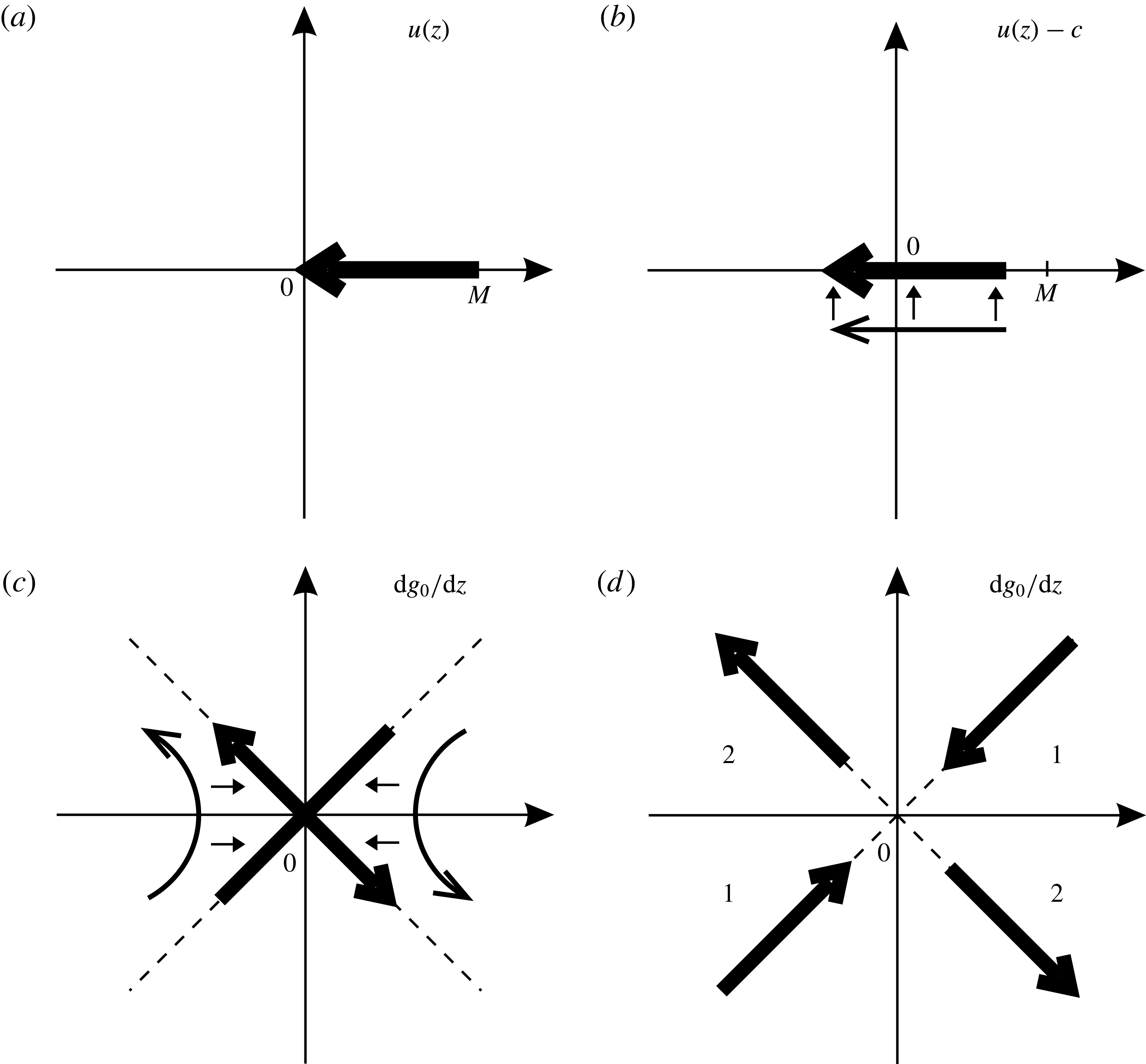
Complex planes
 $u(z)$
(a);
 $u(z)-c$
(b);
 $\sqrt{\text{i}(u-c)/\unicode[STIX]{x1D708}}$
(c) in the case
 $0<c<M$
. Thin arrows show the mappings of
 $0<z<+\infty$
to corresponding planes for
 $c=\text{Re}\,(c)+s\text{i}$
,
 $0<s\ll 1$
, and thick arrows represent their limit as
 $s\rightarrow +0$
. Complex plane
 $\sqrt{\text{i}(u-c)/\unicode[STIX]{x1D708}}$
in the case
 $c<0$
,
 $c>M$
(curves 1, 2, respectively) (d).

First, let us consider waves of phase speeds
 $0<\text{Re}\,c<M$
, and find the value
 $g_{0}^{\prime }(z)$
for
 $z=0$
. At large
 $z$
the radicand takes the form
 $\text{i}H$
, where
 $H$
is a positive real quantity. Therefore, at large
 $z$
, we choose the root branch with the argument
 $-3\unicode[STIX]{x03C0}/4$
. As
 $z$
decreases down to the turning point
 $z_{c}$
, where
 $u(z_{c})-c=0$
, the radicand is equal to zero and the root has the branch point. The WKB solutions are invalid in the neighbourhood of the turning point. To avoid the singularity at real
 $z$
, it is necessary to represent the phase speed as
 $c=\text{Re}\,(c)+s\text{i}$
, where
 $s$
is a small positive quantity; in this case the real
 $z$
axis is located below the point
 $z_{c}$
(§ 3.2). In figure 3(a,b) the values of the functions
 $u(z)$
and
 $u(z)-c$
are illustrated in the complex planes, the arrows show variations of the functions as
 $z$
decreases from
 $+\infty$
to 0. In figure 3(c) the values of the two branches
 $\sqrt{\text{i}(u-c)/\unicode[STIX]{x1D708}}$
are shown. Due to the radiation condition, we choose a branch that is located to the left of the imaginary axis. Finally, as
 $s$
tends to zero, for real
 $c$
we obtain
 $$\begin{eqnarray}g_{0}^{\prime }(0)=\sqrt{{\displaystyle \frac{c}{\unicode[STIX]{x1D708}}}}\times \text{e}^{3\unicode[STIX]{x03C0}\text{i}/4},\quad 0<\text{Re}\,c<M.\end{eqnarray}$$
The cases
 $\text{Re}\,c<0,\text{Re}\,c>M$
are considered similarly, except that there is no need to add a small value
 $s\text{i}$
(figure 3
d). Finally, we obtain:
 $$\begin{eqnarray}g_{0}^{\prime }(0)=\sqrt{\left|{\displaystyle \frac{c}{\unicode[STIX]{x1D708}}}\right|}\times \text{e}^{-3\unicode[STIX]{x03C0}\text{i}/4},\quad \text{Re}\,c<0;\quad g_{0}^{\prime }(0)=\sqrt{{\displaystyle \frac{c}{\unicode[STIX]{x1D708}}}}\times \text{e}^{3\unicode[STIX]{x03C0}\text{i}/4},\quad \text{Re}\,c>M.\end{eqnarray}$$
3.6 Dispersion relation in case of an infinite length plate
Hereafter, for consistency with our previous studies (Vedeneev Reference Vedeneev2013; Bondarev & Vedeneev Reference Bondarev and Vedeneev2016), we will use different scales, which were described in § 2.1, for non-dimensionalisation of the expression (3.21), and to redefine the small parameter
 $\unicode[STIX]{x1D700}=1/\sqrt{R}$
. As a result, by using simple algebra, we obtain
 $$\begin{eqnarray}\displaystyle \unicode[STIX]{x03C0}(z) & = & \displaystyle \left[1+\unicode[STIX]{x1D700}\frac{Q}{|\sqrt{k}|}\left|\frac{\displaystyle c}{\displaystyle \unicode[STIX]{x1D708}}\right|^{-1/2}(M\unicode[STIX]{x1D6FF})^{1/2}\left(-\frac{\displaystyle u^{\prime }(0)}{\displaystyle c}+\frac{\displaystyle T(0)}{\displaystyle \unicode[STIX]{x1D707}c^{2}}\unicode[STIX]{x03C0}_{inv}(0)\right)\right]\unicode[STIX]{x03C0}_{inv}(z)\nonumber\\ \displaystyle & & \displaystyle +\,O(\unicode[STIX]{x1D700}\unicode[STIX]{x1D707}^{2})+O(\unicode[STIX]{x1D700}^{2}),\end{eqnarray}$$
 $$\begin{eqnarray}\unicode[STIX]{x03C0}_{inv}(z)=-\frac{\text{i}\unicode[STIX]{x1D707}}{k}\left[{\displaystyle \frac{(u-c)\unicode[STIX]{x1D711}_{inv}^{\prime }-u^{\prime }\unicode[STIX]{x1D711}_{inv}}{T-M^{2}(u-c)^{2}}}\right],\end{eqnarray}$$
where
 $$\begin{eqnarray}\left.\begin{array}{@{}c@{}}Q=\text{e}^{-3\unicode[STIX]{x03C0}\text{i}/4},\quad \text{Re}\,c>0,\\ Q=\text{e}^{3\unicode[STIX]{x03C0}\text{i}/4},\quad \text{Re}\,c<0,\end{array}\right\}\end{eqnarray}$$
and
 $\unicode[STIX]{x1D707}$
is the density of the mean flow rated to the plate material density. Note that, due to the definition of the Reynolds number,
 $\unicode[STIX]{x1D708}(z)$
is the kinematic viscosity rated to its value in the mean flow.
Substituting the expression for the pressure perturbation (3.25) into (2.4), we obtain the explicit form of the dispersion relation for a plate in a boundary layer flow:
 $$\begin{eqnarray}\displaystyle {\mathcal{D}}(k,\unicode[STIX]{x1D714}) & = & \displaystyle Dk^{4}+M_{w}^{2}k^{2}-\unicode[STIX]{x1D714}^{2}\nonumber\\ \displaystyle & & \displaystyle +\,\unicode[STIX]{x1D707}\left[1+\unicode[STIX]{x1D700}\frac{Q}{|\sqrt{k}|}\left|\frac{\displaystyle c}{\displaystyle \unicode[STIX]{x1D708}}\right|^{-1/2}(M\unicode[STIX]{x1D6FF})^{1/2}\left(-\frac{\displaystyle u^{\prime }(0)}{\displaystyle c}+\frac{\displaystyle T(0)}{\displaystyle c^{2}}\unicode[STIX]{x1D6F1}_{inv}(0)\right)\right]\unicode[STIX]{x1D6F1}_{inv}(0)\nonumber\\ \displaystyle & & \displaystyle +\,O(\unicode[STIX]{x1D700}\unicode[STIX]{x1D707}^{2})+O(\unicode[STIX]{x1D700}^{2})=0,\end{eqnarray}$$
where
 $$\begin{eqnarray}\unicode[STIX]{x1D6F1}_{inv}=\frac{\unicode[STIX]{x03C0}_{inv}}{\unicode[STIX]{x1D707}}=-\frac{\text{i}}{k}\left[{\displaystyle \frac{(u-c)\unicode[STIX]{x1D711}_{inv}^{\prime }-u^{\prime }\unicode[STIX]{x1D711}_{inv}}{T-M^{2}(u-c)^{2}}}\right].\end{eqnarray}$$
By using asymptotic expansions for the solutions of (3.28) in
 $\unicode[STIX]{x1D700}$
and
 $\unicode[STIX]{x1D707}$
(the case of long waves), Bondarev & Vedeneev (Reference Bondarev and Vedeneev2017) studied the effect of viscosity on travelling waves in an infinite length plate for small boundary layer thickness. It was shown that the effect of the finiteness of the Reynolds number (compared with the inviscid approximation) can have a destabilising and a stabilising effect, depending on the phase speed value of the perturbation wave. Namely, in the case of
 $0<\text{Re}\,c<M-1$
the viscous term leads to an increase of the growth rate of the perturbations; on the contrary, in the case of
 $M-1<\text{Re}\,c<M+1$
a viscous term always has a stabilising effect. For an arbitrary thicknesses of the boundary layer, the case of a long wave was analytically investigated for all possible values of phase speed. It was shown that the viscosity can have both a stabilising and destabilising effect.
In the next section we will investigate the influence of the viscous boundary layer perturbations on the stability of finite plates, which is the main goal of this study.
4 Single-mode flutter of finite plates with consideration of viscous perturbations
In this section, we assume that the plate length is finite but sufficiently large so that Kulikovskii’s instability criterion (§ 2.2) may be used, and the Reynolds number is large but finite.
4.1 Method for solving asymptotic eigenvalue problem
Applying Kulikovskii’s global instability criterion, the position of the curve
 $\unicode[STIX]{x1D6FA}$
in the
 $\unicode[STIX]{x1D714}$
-plane was calculated by Bondarev & Vedeneev (Reference Bondarev and Vedeneev2016) in the case of inviscid shear layer approximation for the generalised convex profile and a profile with a generalised inflection point for various thicknesses of the boundary layer. We denote this curve as
 $\unicode[STIX]{x1D6FA}_{inv}$
. As before, the index ‘inv’ refers to the inviscid approximation.
Now we will investigate how the shape of the
 $\unicode[STIX]{x1D6FA}$
-curve changes in the viscous approximation, which we denote as
 $\unicode[STIX]{x1D6FA}_{v}$
, i.e. how the viscosity will affect the growth rate (or damping rate) of the perturbations. Let us introduce a complex function
 $F(\unicode[STIX]{x1D714},\unicode[STIX]{x1D700})=k_{2}(\unicode[STIX]{x1D714},\unicode[STIX]{x1D700})-k_{3}(\unicode[STIX]{x1D714},\unicode[STIX]{x1D700})$
, where
 $k_{2}$
and
 $k_{3}$
are the spatial roots of the dispersion relation (3.28) corresponding to forward- and backward-travelling waves, as defined in § 2.2.
Taylor expansion of
 $F(\unicode[STIX]{x1D714},\unicode[STIX]{x1D700})$
around a point
 $(\unicode[STIX]{x1D714}_{0},0)$
, where
 $\unicode[STIX]{x1D714}_{0}\in \unicode[STIX]{x1D6FA}_{inv}$
, has the form:
 $$\begin{eqnarray}F(\unicode[STIX]{x1D714},\unicode[STIX]{x1D700})=F(\unicode[STIX]{x1D714}_{0},0)+\left.\unicode[STIX]{x0394}\unicode[STIX]{x1D714}\frac{\displaystyle \unicode[STIX]{x2202}F}{\displaystyle \unicode[STIX]{x2202}\unicode[STIX]{x1D714}}\right|_{\begin{smallmatrix}\unicode[STIX]{x1D700}=0\\ \unicode[STIX]{x1D714}=\unicode[STIX]{x1D714}_{0}\end{smallmatrix}}+\left.\unicode[STIX]{x1D700}\frac{\displaystyle \unicode[STIX]{x2202}F}{\displaystyle \unicode[STIX]{x2202}\unicode[STIX]{x1D700}}\right|_{\begin{smallmatrix}\unicode[STIX]{x1D700}=0\\ \unicode[STIX]{x1D714}=\unicode[STIX]{x1D714}_{0}\end{smallmatrix}}+o(\unicode[STIX]{x0394}\unicode[STIX]{x1D714},\unicode[STIX]{x1D700}),\quad \unicode[STIX]{x1D714}=\unicode[STIX]{x1D714}_{0}+\unicode[STIX]{x0394}\unicode[STIX]{x1D714}.\end{eqnarray}$$
Note that the curve
 $\unicode[STIX]{x1D6FA}_{v}$
for a fixed
 $\unicode[STIX]{x1D700}=1/\sqrt{R}$
is given by the equation
 $\text{Im}\,F(\unicode[STIX]{x1D714},\unicode[STIX]{x1D700})=0$
. Simplifying this expression and neglecting infinitesimal terms, we obtain:
 $$\begin{eqnarray}\text{Im}\,\left(\left.\unicode[STIX]{x0394}\unicode[STIX]{x1D714}\frac{\displaystyle \unicode[STIX]{x2202}F}{\displaystyle \unicode[STIX]{x2202}\unicode[STIX]{x1D714}}\right|_{\begin{smallmatrix}\unicode[STIX]{x1D700}=0\\ \unicode[STIX]{x1D714}=\unicode[STIX]{x1D714}_{0}\end{smallmatrix}}+\left.\unicode[STIX]{x1D700}\frac{\displaystyle \unicode[STIX]{x2202}F}{\displaystyle \unicode[STIX]{x2202}\unicode[STIX]{x1D700}}\right|_{\begin{smallmatrix}\unicode[STIX]{x1D700}=0\\ \unicode[STIX]{x1D714}=\unicode[STIX]{x1D714}_{0}\end{smallmatrix}}\right)=0.\end{eqnarray}$$
We are interested in the offset of the
 $\unicode[STIX]{x1D6FA}_{v}$
-curve from
 $\unicode[STIX]{x1D6FA}_{inv}$
, i.e. for a given
 $\text{Re}\,\unicode[STIX]{x1D714}_{0}$
,
 $\unicode[STIX]{x1D714}_{0}\in \unicode[STIX]{x1D6FA}_{inv}$
, we search for the value
 $\unicode[STIX]{x0394}\unicode[STIX]{x1D714}$
, such that
 $\unicode[STIX]{x1D714}=\unicode[STIX]{x1D714}_{0}+\unicode[STIX]{x0394}\unicode[STIX]{x1D714}$
lies on the
 $\unicode[STIX]{x1D6FA}_{v}$
-curve, where
 $\unicode[STIX]{x0394}\unicode[STIX]{x1D714}=\text{i}A$
,
 $A\in \mathbb{R}$
. If
 $A>0$
(
 $A<0$
) then the viscosity has a destabilising (stabilising) effect. Using the expression (4.2), we obtain
 $$\begin{eqnarray}A=-\unicode[STIX]{x1D700}\left[\text{Im}\,\frac{\displaystyle \unicode[STIX]{x2202}F}{\displaystyle \unicode[STIX]{x2202}\unicode[STIX]{x1D700}}\left(\text{Re}\,\frac{\displaystyle \unicode[STIX]{x2202}F}{\displaystyle \unicode[STIX]{x2202}\unicode[STIX]{x1D714}}\right)^{-1}\right]_{\begin{smallmatrix}\unicode[STIX]{x1D700}=0\\ \unicode[STIX]{x1D714}=\unicode[STIX]{x1D714}_{0}\end{smallmatrix}}.\end{eqnarray}$$
First, let us find
 $\text{Im}\,(\displaystyle \unicode[STIX]{x2202}F/\displaystyle \unicode[STIX]{x2202}\unicode[STIX]{x1D700})$
. According to the definition of the function
 $F$
:
 $$\begin{eqnarray}\text{Im}\,\left.\frac{\displaystyle \unicode[STIX]{x2202}F}{\displaystyle \unicode[STIX]{x2202}\unicode[STIX]{x1D700}}\right|_{\begin{smallmatrix}\unicode[STIX]{x1D700}=0\\ \unicode[STIX]{x1D714}=\unicode[STIX]{x1D714}_{0}\end{smallmatrix}}=\text{Im}\,\left.\frac{\displaystyle \unicode[STIX]{x2202}k_{2}}{\displaystyle \unicode[STIX]{x2202}\unicode[STIX]{x1D700}}\right|_{\begin{smallmatrix}\unicode[STIX]{x1D700}=0\\ \unicode[STIX]{x1D714}=\unicode[STIX]{x1D714}_{0}\end{smallmatrix}}-\text{Im}\,\left.\frac{\displaystyle \unicode[STIX]{x2202}k_{3}}{\displaystyle \unicode[STIX]{x2202}\unicode[STIX]{x1D700}}\right|_{\begin{smallmatrix}\unicode[STIX]{x1D700}=0\\ \unicode[STIX]{x1D714}=\unicode[STIX]{x1D714}_{0}\end{smallmatrix}},\end{eqnarray}$$
where
 $k_{j}(\unicode[STIX]{x1D714},\unicode[STIX]{x1D700}),j=2,3$
are defined by (2.4)
 $$\begin{eqnarray}k_{j}=(-1)^{j}\sqrt{\frac{-M_{w}^{2}+\sqrt{M_{w}^{4}+4D(\unicode[STIX]{x1D714}^{2}-\unicode[STIX]{x03C0}_{j}(0,\unicode[STIX]{x1D700}))}}{2D}}.\end{eqnarray}$$
Substitution of (4.5) and (3.25) into (4.4) yields
 $$\begin{eqnarray}\displaystyle & & \displaystyle \text{Im}\,\left.\frac{\displaystyle \unicode[STIX]{x2202}F}{\displaystyle \unicode[STIX]{x2202}\unicode[STIX]{x1D700}}\right|_{\begin{smallmatrix}\unicode[STIX]{x1D700}=0\\ \unicode[STIX]{x1D714}=\unicode[STIX]{x1D714}_{0}\end{smallmatrix}}=-\frac{1}{2}(M\unicode[STIX]{x1D6FF})^{1/2}\nonumber\\ \displaystyle & & \displaystyle \quad \times \,\text{Im}\,\left[\frac{(k_{2}|\sqrt{k_{2}}|)^{-1}}{\sqrt{M_{w}^{4}+4D(\unicode[STIX]{x1D714}^{2}-\unicode[STIX]{x03C0}_{2,inv}(0))}}\left|\frac{\displaystyle c_{2}}{\displaystyle \unicode[STIX]{x1D708}}\right|^{-1/2}\text{e}^{-3\unicode[STIX]{x03C0}\text{i}/4}\left(\!-\frac{\displaystyle u^{\prime }(0)}{\displaystyle c_{2}}+\frac{\displaystyle T(0)}{\displaystyle \unicode[STIX]{x1D707}c_{2}^{2}}\unicode[STIX]{x03C0}_{2,inv}(0)\!\right)\unicode[STIX]{x03C0}_{2,inv}(0)\right.\nonumber\\ \displaystyle & & \displaystyle \quad -\left.\frac{(k_{3}|\sqrt{k_{3}}|)^{-1}}{\sqrt{M_{w}^{4}+4D(\unicode[STIX]{x1D714}^{2}-\unicode[STIX]{x03C0}_{3,inv}(0))}}\left|\frac{\displaystyle c_{3}}{\displaystyle \unicode[STIX]{x1D708}}\right|^{-1/2}\!\text{e}^{3\unicode[STIX]{x03C0}\text{i}/4}\!\left(\!-\frac{\displaystyle u^{\prime }(0)}{\displaystyle c_{3}}+\frac{\displaystyle T(0)}{\displaystyle \unicode[STIX]{x1D707}c_{3}^{2}}\unicode[STIX]{x03C0}_{3,inv}(0)\!\right)\!\unicode[STIX]{x03C0}_{3,inv}(0)\right]_{\begin{smallmatrix}\unicode[STIX]{x1D700}=0\\ \unicode[STIX]{x1D714}=\unicode[STIX]{x1D714}_{0}\end{smallmatrix}},\nonumber\\ \displaystyle & & \displaystyle\end{eqnarray}$$
where
 $c_{j}=\unicode[STIX]{x1D714}/k_{j}$
.
To solve the dispersion equation (2.4) in the inviscid case, and find the pressure disturbance
 $\unicode[STIX]{x03C0}_{j,inv}(0)$
,
 $j=1,2$
, we used an iterative procedure. At each iteration we numerically solve the Rayleigh equation to find the velocity perturbation
 $\unicode[STIX]{x1D711}_{j,inv}$
,
 $j=1,2$
, and its derivative. The boundary value problem is reduced to two initial value problems by the standard shooting method, which are both solved along the chosen path, passing below the critical point (according to Lin’s rule, § 3.2), through the Runge–Kutta method. Next, by using formula (3.26), we calculate the inviscid unsteady pressure
 $\unicode[STIX]{x03C0}_{j,inv}(0)$
,
 $j=1,2$
, on the plate surface, which is used in finding the next approximation (4.5) to the solution of the dispersion equation. This method of solving the dispersion equation is described in more detail by Bondarev & Vedeneev (Reference Bondarev and Vedeneev2016).
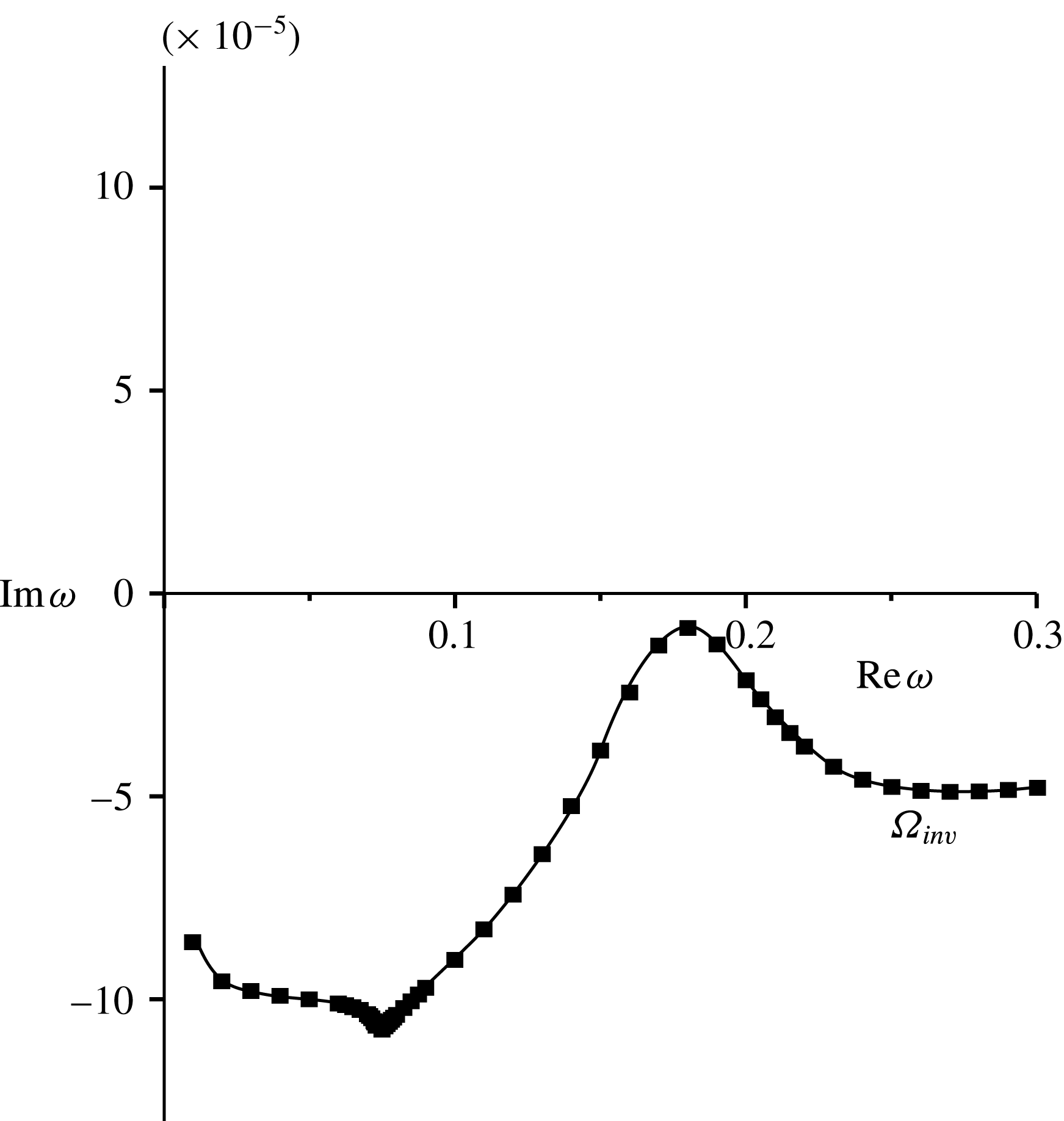
Point-by-point calculation of the curve
 $\unicode[STIX]{x1D6FA}_{inv}$
in the
 $\unicode[STIX]{x1D714}$
-plane.

Next, let us calculate
 $\text{Re}\,(\displaystyle \unicode[STIX]{x2202}F/\displaystyle \unicode[STIX]{x2202}\unicode[STIX]{x1D714})$
. Applying the same numerical procedure that was used by Bondarev & Vedeneev (Reference Bondarev and Vedeneev2016) to find the curve
 $\unicode[STIX]{x1D6FA}_{inv}$
, we calculate
 $\unicode[STIX]{x1D714}_{0}^{j}\in \unicode[STIX]{x1D6FA}_{inv}$
in a point-by-point manner (for example, as shown in figure 4),
 $k_{2}(\unicode[STIX]{x1D714}_{0}^{j})$
,
 $k_{3}(\unicode[STIX]{x1D714}_{0}^{j})$
and
 $F(\unicode[STIX]{x1D714}_{0}^{j})$
. Then
 $\text{Re}\,(\displaystyle \unicode[STIX]{x2202}F/\displaystyle \unicode[STIX]{x2202}\unicode[STIX]{x1D714})_{\unicode[STIX]{x1D700}=0,\unicode[STIX]{x1D714}=\unicode[STIX]{x1D714}_{0}^{j}}$
, where
 $\unicode[STIX]{x1D714}_{0}^{j}\in \unicode[STIX]{x1D6FA}_{inv}$
is calculated numerically, using the first-order finite difference:
 $$\begin{eqnarray}\text{Re}\,\left.\frac{\displaystyle \unicode[STIX]{x2202}F}{\displaystyle \unicode[STIX]{x2202}\unicode[STIX]{x1D714}}\right|_{\begin{smallmatrix}\unicode[STIX]{x1D700}=0\\ \unicode[STIX]{x1D714}=\unicode[STIX]{x1D714}_{0}^{j}\end{smallmatrix}}=\text{Re}\,\left(\frac{F(\unicode[STIX]{x1D714}_{0}^{j})-F(\unicode[STIX]{x1D714}_{0}^{j-1})}{\unicode[STIX]{x1D714}_{0}^{j}-\unicode[STIX]{x1D714}_{0}^{j-1}}\right).\end{eqnarray}$$
4.2 Results
As examples, we considered two boundary layer profiles representing a typical generalised convex profile and a profile having generalised inflection points (the same profiles were studied by Bondarev & Vedeneev (Reference Bondarev and Vedeneev2016).
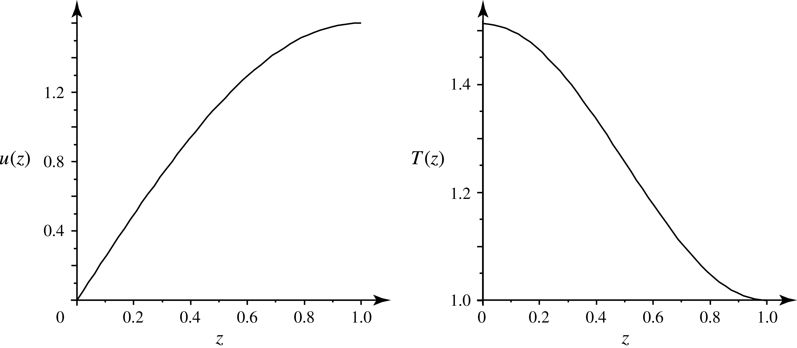
(i) The generalised convex profile. The velocity distribution is as follows:
 $$\begin{eqnarray}u(z)=M\sin \left(\frac{\unicode[STIX]{x03C0}}{2}\frac{z}{\unicode[STIX]{x1D6FF}}\right)\end{eqnarray}$$
for
 $M=1.6$
and
 $$\begin{eqnarray}D=23.9,\quad M_{w}=0,\quad \unicode[STIX]{x1D707}=0.00012,\quad \unicode[STIX]{x1D6FE}=1.4,\end{eqnarray}$$
which correspond to a steel untensioned plate at 3000 m, or an aluminium plate at 11 000 m above sea level. For simplicity, in all examples hereafter we assume that the Prandtl number
 $Pr=1$
and the plate is heat insulated so that the steady temperature profile
 $T(u)$
is given by the expression (Schlichting Reference Schlichting1960):
 $$\begin{eqnarray}T(u)=1+\frac{\unicode[STIX]{x1D6FE}-1}{2}(M^{2}-u^{2}).\end{eqnarray}$$
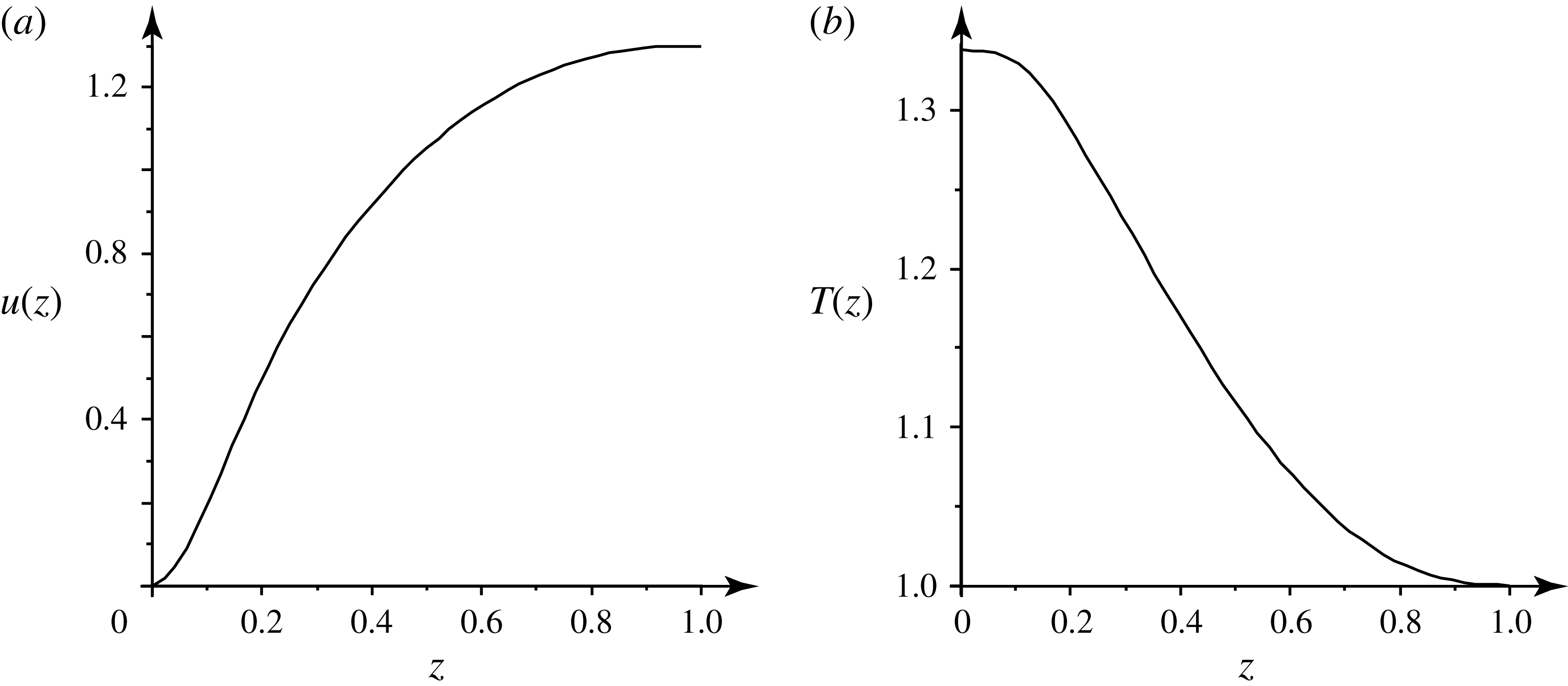
The velocity and temperature distributions (4.8) and (4.10) are shown in figure 5.

(ii) The boundary layer profile with a generalised inflection point:
 $$\begin{eqnarray}u(z)=M\left(1-\left(1-\frac{z}{\unicode[STIX]{x1D6FF}}\right)^{2.4}\right)\times \cos \left(0.7\left(1-\frac{z}{\unicode[STIX]{x1D6FF}}\right)^{7}\right)^{7}\end{eqnarray}$$
for
 $M=1.3$
, parameters (4.9a–d
) and the temperature profile (4.10), which are shown in figure 6. Although the velocity profile (4.11) looks sophisticated, it simply represents a function with one generalised inflection point located in the supersonic (with respect to the mean flow) part of the layer.

4.2.1 Results for generalised convex boundary layer profile
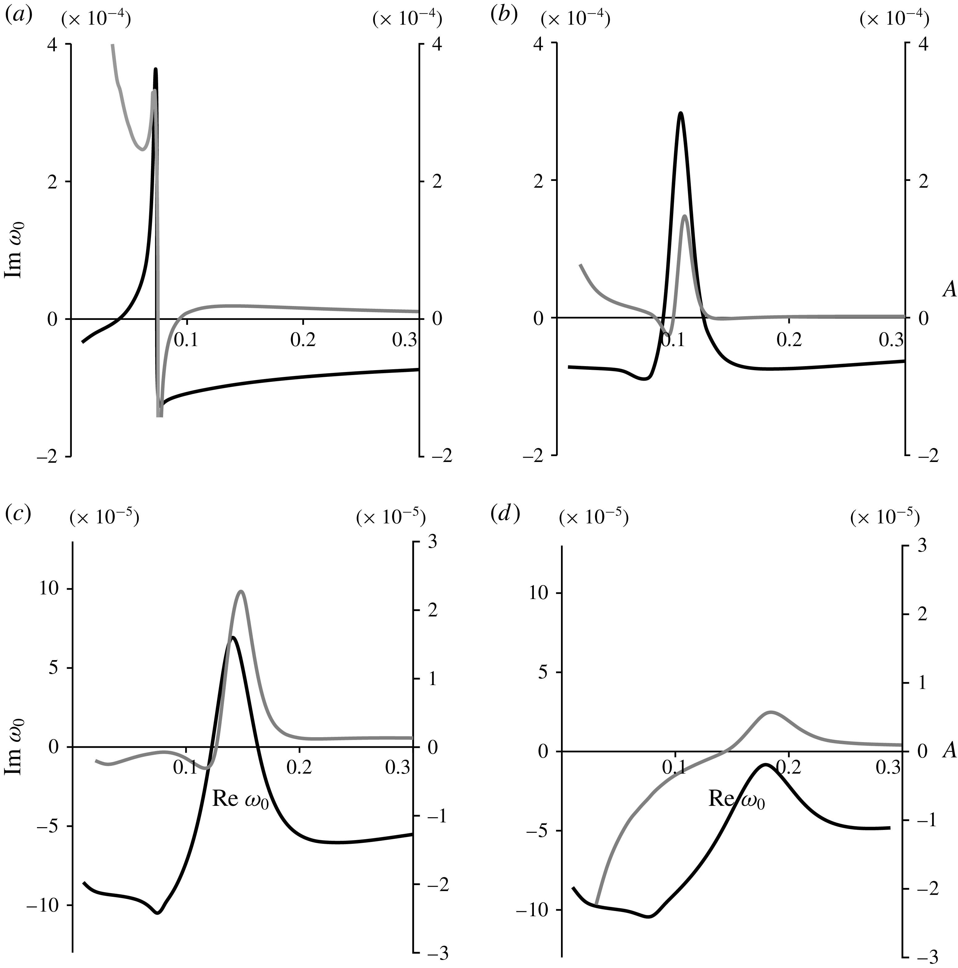
Grey and black lines represent the viscous term
 $A$
versus
 $\text{Re}\,\unicode[STIX]{x1D714}_{0}$
and curve
 $\unicode[STIX]{x1D6FA}_{inv}$
(Bondarev & Vedeneev Reference Bondarev and Vedeneev2016) in the
 $\unicode[STIX]{x1D714}$
-plane, respectively, for the boundary layer profile (4.8), (4.10) and boundary layer thickness
 $\unicode[STIX]{x1D6FF}=0.1$
(a),
 $\unicode[STIX]{x1D6FF}=2$
(b),
 $\unicode[STIX]{x1D6FF}=3$
(c),
 $\unicode[STIX]{x1D6FF}=4$
(d).

Let us now investigate the viscous growth rates
 $\text{Im}\,\unicode[STIX]{x0394}\unicode[STIX]{x1D714}=A$
in the case of the generalised convex boundary layer profile, which is defined by the velocity profile (4.8) and the temperature profile (4.10). The value of the kinematic viscosity
 $\unicode[STIX]{x1D708}(0)=T(0)^{1.75}\approx 2.0616$
according to Sutherland’s formula for the dynamic viscosity of air and the perfect gas law for the density–temperature relation. For visualisation of the results,
 $\unicode[STIX]{x1D700}=0.01$
was taken in the calculations; however, as can be seen from (4.3), the qualitative effect of viscosity, stabilising or destabilising, does not depend on
 $\unicode[STIX]{x1D700}$
.
Figure 7 shows the viscous term
 $A$
versus
 $\text{Re}\,\unicode[STIX]{x1D714}_{0}$
for different boundary layer thicknesses. The following observations are made:
(i) For thin boundary layer thickness (
$\unicode[STIX]{x1D6FF}=0.1$
, figure 7
a), the shown frequency range corresponds to a destabilising effect of viscosity, except for
$\text{Re}\,\unicode[STIX]{x1D714}_{0}\in [0.076;0.093]$
. The highest viscous growth rates take place at
$\text{Re}\,\unicode[STIX]{x1D714}_{0}<0.076$
, while for
$\text{Re}\,\unicode[STIX]{x1D714}_{0}>0.093$
the growth rates tend to zero.(ii) For increased boundary layer thickness (
$\unicode[STIX]{x1D6FF}=2$
, figure 7
b), there are two small frequency segments,
$\text{Re}\,\unicode[STIX]{x1D714}_{0}\in [0.086;0.101]$
and
$\text{Re}\,\unicode[STIX]{x1D714}_{0}\in [0.135;0.17]$
, where the viscous term
$A$
is negative. We note a strongly marked maximum at
$\text{Re}\,\unicode[STIX]{x1D714}_{0}\approx 0.11$
. For
$\text{Re}\,\unicode[STIX]{x1D714}_{0}>0.17$
viscous growth rates are close to zero.(iii) For
$\unicode[STIX]{x1D6FF}\geqslant 3$
(figure 7
c), there is only one frequency threshold separating the stabilising and destabilising effect of viscosity. In the case of
$\unicode[STIX]{x1D6FF}=3$
the maximum viscous growth rate
$A$
is lower, and the frequency range of the growing eigenmodes is wider than for
$\unicode[STIX]{x1D6FF}=2$
.(iv) For thick boundary layers (
$\unicode[STIX]{x1D6FF}\geqslant 4$
, figure 7
d), the maximum viscous growth rate continues decreasing down to zero. However, for all considered thicknesses
$\unicode[STIX]{x1D6FF}$
there remains a frequency range where the viscosity effect is destabilising.








4.2.2 Results for profile with a generalised inflection point
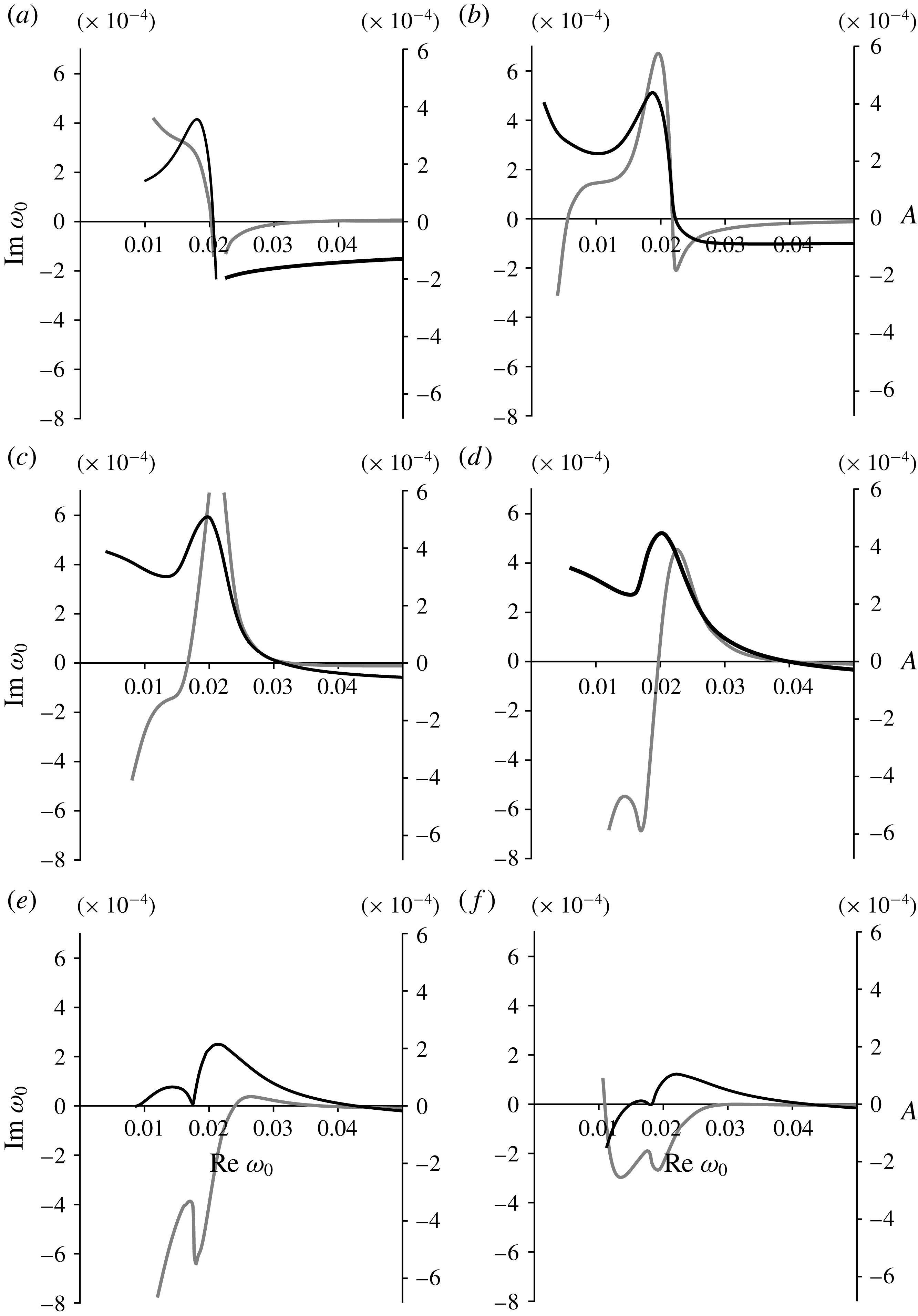
Grey and black lines represent the viscous term
 $A$
versus
 $\text{Re}\,\unicode[STIX]{x1D714}_{0}$
and curve
 $\unicode[STIX]{x1D6FA}_{inv}$
(Bondarev & Vedeneev Reference Bondarev and Vedeneev2016) in the
 $\unicode[STIX]{x1D714}$
-plane, respectively, for the boundary layer profile (4.11), (4.10) and boundary layer thickness
 $\unicode[STIX]{x1D6FF}=0.1$
(a),
 $\unicode[STIX]{x1D6FF}=2$
(b),
 $\unicode[STIX]{x1D6FF}=4$
(c),
 $\unicode[STIX]{x1D6FF}=6$
(d),
 $\unicode[STIX]{x1D6FF}=10$
(e),
 $\unicode[STIX]{x1D6FF}=14$
(f).

Next, let us consider a boundary layer profile with a generalised inflection point defined by (4.11) and (4.10), which gives
 $\unicode[STIX]{x1D708}(0)\approx 1.6645$
. As before, for visualisation purposes we take
 $\unicode[STIX]{x1D700}=0.01$
. The calculated viscous term
 $A$
versus
 $\text{Re}\,\unicode[STIX]{x1D714}_{0}$
is shown in figure 8. The results can be summarised as follows:
(i) For small
$\unicode[STIX]{x1D6FF}=0.1$
(figure 8
a), there is a similar behaviour to the case of the generalised convex profile: all frequencies correspond to positive viscous growth rates, except for
$\text{Re}\,\unicode[STIX]{x1D714}_{0}\in [0.02;0.037]$
. The highest viscous growth rates correspond to low frequencies (
$\text{Re}\,\unicode[STIX]{x1D714}_{0}<0.02$
), while for
$\text{Re}\,\unicode[STIX]{x1D714}_{0}>0.037$
growth rates are close to zero, but stay positive.(ii) For the boundary layer thickness
$\unicode[STIX]{x1D6FF}=2$
(figure 8
b), there is a single frequency range with a destabilising effect of the viscosity
$\text{Re}\,\unicode[STIX]{x1D714}_{0}\in [0.006;0.022]$
, with a pronounced maximum viscous growth rate at
$\text{Re}\,\unicode[STIX]{x1D714}_{0}\approx 0.02$
. For
$\text{Re}\,\unicode[STIX]{x1D714}_{0}>0.022$
there is a dip into the stability region
$A<0$
. After the dip, viscous growth rates tend to zero as
$\text{Re}\,\unicode[STIX]{x1D714}_{0}$
increases.(iii) For higher
$\unicode[STIX]{x1D6FF}$
, the maximum viscous growth rate decreases as
$\unicode[STIX]{x1D6FF}$
increases (figure 8
c–e) and almost disappears at
$\unicode[STIX]{x1D6FF}=14$
(figure 8
f).(iv) For a very thick boundary layer
$\unicode[STIX]{x1D6FF}=14$
viscous growth appears at small
$\text{Re}\,\unicode[STIX]{x1D714}_{0}$
.







Comparing the results of the inviscid approximation (
 $\unicode[STIX]{x1D6FA}_{inv}$
) with the viscous term effect (figures 7 and 8), we notice that frequencies
 $\text{Re}\,\unicode[STIX]{x1D714}_{0}$
corresponding to the maximum ‘inviscid’ and ‘viscous’ growth rates are close to each other for moderate boundary layer thicknesses. Hence, if the inviscid shear layer destabilises the plate, i.e. the plate flutters, the viscosity surprisingly yields even more destabilisation. To explain this effect, the relation between the ‘inviscid’ and ‘viscous’ maximum growth rates is studied below.
4.3 The relation between growth rate peaks produced by inviscid and viscous terms
First, let us find the connection between growth rates and pressure disturbances in the inviscid and viscous approaches. We will assume that
 $\unicode[STIX]{x1D707}$
, which is the ratio of the mean flow density to the plate material density, is a small parameter (typically of the order of
 $10^{-3}$
or less). Let us also assume that
 $\unicode[STIX]{x1D714}=\unicode[STIX]{x1D714}_{R}+\text{i}\unicode[STIX]{x1D714}_{I}$
,
 $\unicode[STIX]{x1D714}_{R}\gg |\unicode[STIX]{x1D714}_{I}|$
and
 $\unicode[STIX]{x1D714}_{R}\gg \unicode[STIX]{x1D707}$
, which is valid for single-mode flutter (Vedeneev Reference Vedeneev2005, Reference Vedeneev2013). Then from (2.4) the Taylor expansion yields
 $$\begin{eqnarray}k_{j}(\unicode[STIX]{x1D714}_{R}+\text{i}\unicode[STIX]{x1D714}_{I},\unicode[STIX]{x1D707},\unicode[STIX]{x1D700})=k_{j}(\unicode[STIX]{x1D714}_{R},0,\unicode[STIX]{x1D700})+\text{i}\unicode[STIX]{x1D714}_{I}\left.\frac{\unicode[STIX]{x2202}k_{j}}{\unicode[STIX]{x2202}\unicode[STIX]{x1D714}}\right|_{\begin{smallmatrix}\unicode[STIX]{x1D714}_{I}=0\\ \unicode[STIX]{x1D707}=0\end{smallmatrix}}+\unicode[STIX]{x1D707}\left.\frac{\unicode[STIX]{x2202}k_{j}}{\unicode[STIX]{x2202}\unicode[STIX]{x1D707}}\right|_{\begin{smallmatrix}\unicode[STIX]{x1D714}_{I}=0\\ \unicode[STIX]{x1D707}=0\end{smallmatrix}},\end{eqnarray}$$
where
 $$\begin{eqnarray}\displaystyle & \displaystyle \left.\frac{\unicode[STIX]{x2202}k_{j}}{\unicode[STIX]{x2202}\unicode[STIX]{x1D714}}\right|_{\begin{smallmatrix}\unicode[STIX]{x1D714}_{I}=0\\ \unicode[STIX]{x1D707}=0\end{smallmatrix}}=\left.\frac{\displaystyle \unicode[STIX]{x1D714}}{\displaystyle k_{j}(M_{w}^{2}+2Dk_{j}^{2})}\right|_{\begin{smallmatrix}\unicode[STIX]{x1D714}_{I}=0\\ \unicode[STIX]{x1D707}=0\end{smallmatrix}}, & \displaystyle\end{eqnarray}$$
 $$\begin{eqnarray}\displaystyle & \displaystyle \left.\frac{\unicode[STIX]{x2202}k_{j}}{\unicode[STIX]{x2202}\unicode[STIX]{x1D707}}\right|_{\begin{smallmatrix}\unicode[STIX]{x1D714}_{I}=0\\ \unicode[STIX]{x1D707}=0\end{smallmatrix}}=-\left.\frac{\displaystyle \unicode[STIX]{x1D6F1}_{j}(0)}{\displaystyle 2k_{j}(M_{w}^{2}+2Dk_{j}^{2})}\right|_{\begin{smallmatrix}\unicode[STIX]{x1D714}_{I}=0\\ \unicode[STIX]{x1D707}=0\end{smallmatrix}}. & \displaystyle\end{eqnarray}$$
Then, we substitute (4.12) into Kulikovskii’s global instability equation
 $$\begin{eqnarray}\text{Im}\,k_{2}(\unicode[STIX]{x1D714},\unicode[STIX]{x1D707},\unicode[STIX]{x1D700})-\text{Im}\,k_{3}(\unicode[STIX]{x1D714},\unicode[STIX]{x1D707},\unicode[STIX]{x1D700})=0\end{eqnarray}$$
and obtain the equation for
 $\unicode[STIX]{x1D714}_{I}$
, which is valid for any
 $\unicode[STIX]{x1D700}$
 $$\begin{eqnarray}\unicode[STIX]{x1D714}_{I}=\frac{\unicode[STIX]{x1D707}}{4\unicode[STIX]{x1D714}_{R}}\text{Im}\,(\unicode[STIX]{x1D6F1}_{2}(0)+\unicode[STIX]{x1D6F1}_{3}(0))_{\begin{smallmatrix}\unicode[STIX]{x1D714}_{I}=0\\ \unicode[STIX]{x1D707}=0.\end{smallmatrix}}\end{eqnarray}$$
Thus, the growth rate of the finite plate eigenmode depends on the sum of pressures
 $\unicode[STIX]{x1D6F1}_{2}$
and
 $\unicode[STIX]{x1D6F1}_{3}$
produced by downstream-travelling and upstream-travelling plate waves, respectively.
Therefore, for
 $\unicode[STIX]{x1D714}_{0}\in \unicode[STIX]{x1D6FA}_{inv}$
in an inviscid approximation (
 $\unicode[STIX]{x1D700}=0$
) we have:
 $$\begin{eqnarray}\displaystyle \text{Im}\,\unicode[STIX]{x1D714}_{0} & = & \displaystyle \frac{\unicode[STIX]{x1D707}}{4\text{Re}\,\unicode[STIX]{x1D714}_{0}}\text{Im}\,(\unicode[STIX]{x1D6F1}_{2,inv}(0)+\unicode[STIX]{x1D6F1}_{3,inv}(0))_{\begin{smallmatrix}\text{Im}\,\unicode[STIX]{x1D714}_{0}=0\\ \unicode[STIX]{x1D707}=0\end{smallmatrix}}\nonumber\\ \displaystyle & = & \displaystyle \frac{\unicode[STIX]{x1D707}}{4\text{Re}\,\unicode[STIX]{x1D714}_{0}}\text{Im}\,(\unicode[STIX]{x1D6F1}_{2,inv}(0)+\unicode[STIX]{x1D6F1}_{3,inv}(0))_{\begin{smallmatrix}\text{Im}\,\unicode[STIX]{x1D714}_{0}\neq 0\\ \unicode[STIX]{x1D707}\neq 0\end{smallmatrix}}+O(\unicode[STIX]{x1D707}^{2}).\end{eqnarray}$$
For viscous
 $\text{Im}\,\unicode[STIX]{x1D714}\in \unicode[STIX]{x1D6FA}_{v}$
(
 $\unicode[STIX]{x1D700}\not =0$
) we similarly obtain:
 $$\begin{eqnarray}\displaystyle \text{Im}\,\unicode[STIX]{x1D714} & = & \displaystyle \frac{\unicode[STIX]{x1D707}}{4\text{Re}\,\unicode[STIX]{x1D714}_{0}}\text{Im}\,(\unicode[STIX]{x1D6F1}_{2}(0)+\unicode[STIX]{x1D6F1}_{3}(0))_{\begin{smallmatrix}\text{Im}\,\unicode[STIX]{x1D714}=0\\ \unicode[STIX]{x1D707}=0\end{smallmatrix}}\nonumber\\ \displaystyle & = & \displaystyle \frac{\unicode[STIX]{x1D707}}{4\text{Re}\,\unicode[STIX]{x1D714}_{0}}\text{Im}\,(\unicode[STIX]{x1D6F1}_{2}(0)+\unicode[STIX]{x1D6F1}_{3}(0))_{\begin{smallmatrix}\text{Im}\,\unicode[STIX]{x1D714}\neq 0\\ \unicode[STIX]{x1D707}\neq 0\end{smallmatrix}}+O(\unicode[STIX]{x1D707}^{2}).\end{eqnarray}$$
Thus, neglecting the small term
 $O(\unicode[STIX]{x1D707}^{2})$
, we can rewrite (4.17) and (4.18) as
 $$\begin{eqnarray}\displaystyle & \displaystyle \text{Im}\,\unicode[STIX]{x1D714}_{0}=\frac{\unicode[STIX]{x1D707}}{4\text{Re}\,\unicode[STIX]{x1D714}_{0}}\text{Im}\,(\unicode[STIX]{x1D6F1}_{2,inv}(0)+\unicode[STIX]{x1D6F1}_{3,inv}(0))=\frac{1}{4\text{Re}\,\unicode[STIX]{x1D714}_{0}}\text{Im}\,(\unicode[STIX]{x03C0}_{2,inv}(0)+\unicode[STIX]{x03C0}_{3,inv}(0)),\quad & \displaystyle\end{eqnarray}$$
 $$\begin{eqnarray}\displaystyle & \displaystyle \text{Im}\,\unicode[STIX]{x1D714}=\frac{\unicode[STIX]{x1D707}}{4\text{Re}\,\unicode[STIX]{x1D714}_{0}}\text{Im}\,(\unicode[STIX]{x1D6F1}_{2}(0)+\unicode[STIX]{x1D6F1}_{3}(0))=\frac{1}{4\text{Re}\,\unicode[STIX]{x1D714}_{0}}\text{Im}\,(\unicode[STIX]{x03C0}_{2}(0)+\unicode[STIX]{x03C0}_{3}(0)). & \displaystyle\end{eqnarray}$$
According to Vedeneev (Reference Vedeneev2005), the growth of a finite length plate eigenmode in uniform flow occurs due to the growth of the downstream-travelling wave (
 $\text{Im}\,\unicode[STIX]{x03C0}_{2,inv}(0)>0$
), whereas the upstream-travelling wave is always damped (
 $\text{Im}\,\unicode[STIX]{x03C0}_{3,inv}(0)<0$
). Inviscid boundary layer calculations (Bondarev & Vedeneev Reference Bondarev and Vedeneev2016) confirm this statement; namely, the frequencies
 $\text{Re}\,\unicode[STIX]{x1D714}_{0}$
of the maximum growth rates
 $\text{Im}\,\unicode[STIX]{x1D714}_{0}$
and the maximum values of the pressure disturbance
 $\text{Im}\,\unicode[STIX]{x03C0}_{2,inv}(0)$
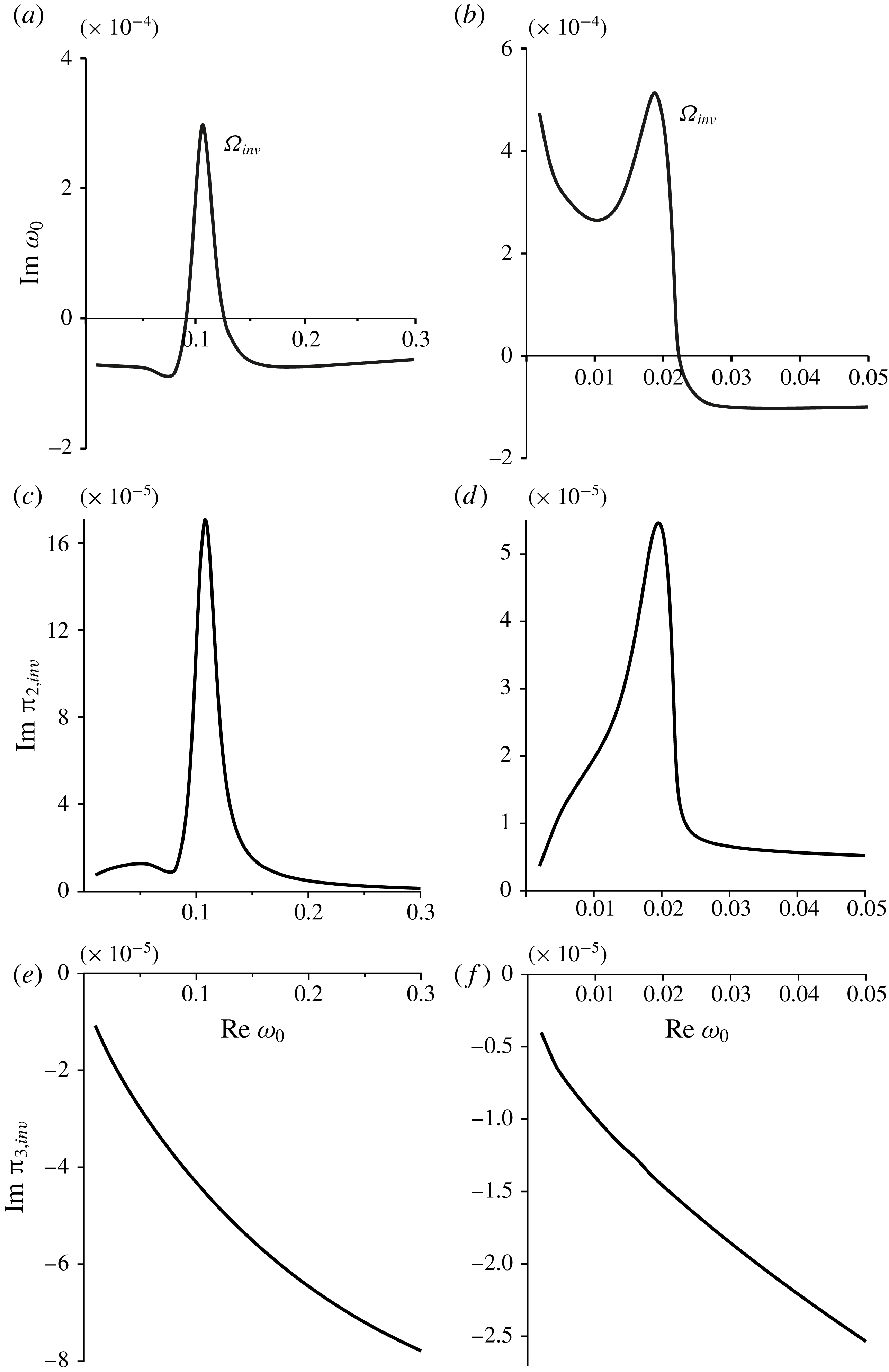
are close to each other. An example is shown in figure 9, where the peak locations of
 $\text{Im}\,\unicode[STIX]{x1D714}_{0}$
and
 $\text{Im}\,\unicode[STIX]{x03C0}_{2,inv}(0)$
almost coincide for both types of the boundary layer. In other words, the frequency
 $\text{Re}\,\unicode[STIX]{x1D714}_{0}$
of maximum growth rate in (4.19) is determined only by the pressure perturbation
 $\unicode[STIX]{x03C0}_{2,inv}(0)$
produced by the downstream-travelling wave. Present viscous calculations show that this conclusion is also valid for small
 $\unicode[STIX]{x1D700}$
in the viscous case. Namely, the frequency
 $\text{Re}\,\unicode[STIX]{x1D714}_{0}$
of maximum growth rate is determined only by
 $\unicode[STIX]{x03C0}_{2}(0)$
(4.20).
Curve
 $\unicode[STIX]{x1D6FA}_{inv}$
in the
 $\unicode[STIX]{x1D714}$
-plane (a,b); pressure disturbance
 $\text{Im}\,\unicode[STIX]{x03C0}_{2,inv}$
versus
 $\text{Re}\,\unicode[STIX]{x1D714}$
(c,d); pressure disturbance
 $\text{Im}\,\unicode[STIX]{x03C0}_{3,inv}$
versus
 $\text{Re}\,\unicode[STIX]{x1D714}$
(e,f). The case of the boundary layer profile (4.8), (4.10) (a,c,e); and (4.11), (4.10) (b,d,f); boundary layer thickness
 $\unicode[STIX]{x1D6FF}=2$
.

Let us now investigate how inviscid pressure disturbance
 $\unicode[STIX]{x03C0}_{2,inv}$
affects the viscous pressure disturbance
 $\unicode[STIX]{x03C0}_{2}$
. Denote
 $\text{Im}\,\unicode[STIX]{x03C0}_{2}=\text{Im}\,\unicode[STIX]{x03C0}_{2,inv}+\text{Im}\,\unicode[STIX]{x0394}\unicode[STIX]{x03C0}_{2}$
. Using (3.25), we obtain
 $$\begin{eqnarray}\unicode[STIX]{x0394}\unicode[STIX]{x03C0}_{2}=Q_{1}\text{e}^{-3\unicode[STIX]{x03C0}\text{i}/4}\left(-\frac{\displaystyle u^{\prime }(0)}{\displaystyle c}+\frac{\displaystyle T(0)}{\displaystyle \unicode[STIX]{x1D707}c^{2}}\unicode[STIX]{x03C0}_{inv}\right)\unicode[STIX]{x03C0}_{inv},\quad Q_{1}>0.\end{eqnarray}$$
We fix
 $p_{R}=\text{Re}\,\unicode[STIX]{x03C0}_{2,inv}$
and assume that at the peak of inviscid growth rate
 $p_{I}=\text{Im}\,\unicode[STIX]{x03C0}_{2,inv}>0$
,
 $|p_{R}|\ll |p_{I}|$
, which is in accordance with the calculation results. By neglecting higher-order terms, equation (4.21) transforms to
 $$\begin{eqnarray}\text{Im}\,(\unicode[STIX]{x0394}\unicode[STIX]{x03C0}_{2})\approx Q_{2}p_{I}+Q_{3}p_{I}^{2},\end{eqnarray}$$
where
 $Q_{2,3}>0$
. Thus, from (4.22) we conclude that for peak values of
 $\text{Im}\,\unicode[STIX]{x03C0}_{2,inv}>0$
the viscous shift
 $\text{Im}\,\unicode[STIX]{x0394}\unicode[STIX]{x03C0}_{2}$
is positive and, consequently, the effect of finite Reynolds number is destabilising.
Let us consider an example: the convex boundary layer profile (4.8), (4.10),
 $\unicode[STIX]{x1D6FF}=2$
and the phase speed as
 $c_{2}=0.72544+0.00366\text{i}$
, which corresponds to inviscid calculations with
 $\text{Re}\,\unicode[STIX]{x1D714}_{0}=0.1076$
. We calculate
 $\text{Im}\,\unicode[STIX]{x0394}\unicode[STIX]{x03C0}_{2}$
for different
 $p_{R}$
and
 $p_{I}$
using (4.21) and for simplicity assuming that
 $Q_{1}=1$
. As ‘inviscid’ calculations show that for this boundary layer
 $p_{R}\in [-0.0001;0.0001]$
for all considered
 $\unicode[STIX]{x1D714}_{0}$
, values of
 $p_{R}$
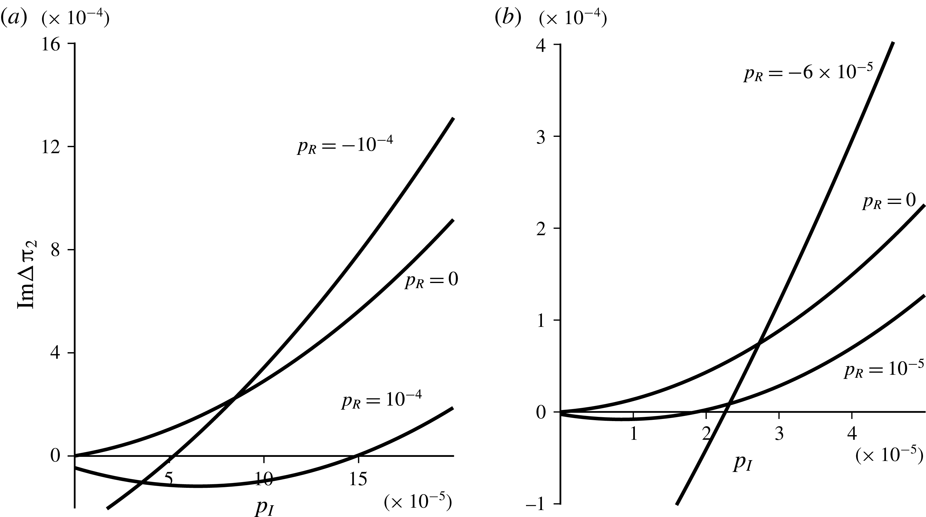
are taken from this range as representative. Figure 10(a) shows that imaginary part of the viscous pressure disturbance
 $\text{Im}\,\unicode[STIX]{x0394}\unicode[STIX]{x03C0}_{2}$
is positive and increases when
 $\text{Im}\,\unicode[STIX]{x03C0}_{2,inv}$
is sufficiently large.
 $\text{Im}\,\unicode[STIX]{x0394}\unicode[STIX]{x03C0}_{2}$
versus
 $p_{I}$
for different
 $p_{R}$
.

Similar conclusions follow from calculations in the case of the profile with a generalised inflection point (4.11), (4.10),
 $\unicode[STIX]{x1D6FF}=2$
and the phase speed
 $c_{2}=0.29960+0.01508\text{i}$
, which corresponds to inviscid calculations with
 $\text{Re}\,\unicode[STIX]{x1D714}_{0}=0.0188$
(figure 10
b). The values of
 $p_{R}\in [-0.00006;0.00001]$
are taken as representative.
Combining the results discussed above, we conclude that the peak value of inviscid growth rate is produced by the peak of inviscid pressure disturbance
 $\text{Im}\,\unicode[STIX]{x03C0}_{2,inv}$
, which, in turn, yields the maximum of
 $\text{Im}\,\unicode[STIX]{x0394}\unicode[STIX]{x03C0}_{2}$
and, hence, of the viscous growth rate
 $A$
. This means that when the inviscid shear layer essentially destabilises the plate (the peak value of the growth rate), viscosity always produces even more destabilisation (i.e. larger growth rate).
5 Discussion and concluding remarks
Let us now review the assumptions used throughout this study. First, we assumed that Reynolds number is finite and large (
 $R\rightarrow \infty$
), which was used in the WKB expansions of the solutions of the equations for the perturbations. The same assumption used in the stability analysis of the boundary layer over a flat rigid plate gives quantitatively correct results for
 $R\sim 1000$
or larger, and yields a qualitatively correct critical Reynolds number
 $R_{cr}=421$
versus the exact value
 $R_{cr}=520$
(Drazin & Reid Reference Drazin and Reid2004, the Reynolds number here is based on displacement thickness). For the plane Poiseuille flow, WKB approximation (corrected by the local turning point approximation) for the flow perturbations yields
 $R_{cr}=5397$
versus the exact value
 $R_{cr}=5772$
(Drazin & Reid Reference Drazin and Reid2004). Note that for the eigenmodes corresponding to
 $R_{cr}$
in both of these flows, the main reason of the deviation of the WKB prediction from the exact value is that the critical layer is merged with the viscous sublayer (triple-deck structure). For a five-deck perturbation structure, which is considered in this study, the WKB expansion is much more accurate. Hence, we may expect that our results are valid for
 $R\sim 1000$
and larger, i.e. they cover most of the boundary layers expected in aeronautical applications.
The other assumption used is the large plate length (
 $L\rightarrow \infty$
), which was employed in Kulikovskii’s instability criterion. A detailed comparison between the results predicted by this criterion and the numerical solution of the full aeroelastic problem (Vedeneev Reference Vedeneev2012, Reference Vedeneev2016) shows that for the two-dimensional problem the calculated flutter boundary is accurate for
 $L\sim 100$
and larger (the panel length is non-dimensionalised by its thickness), which covers most of the skin panel dimensions used in flight vehicles. This estimate was obtained for the uniform flow analysis. For lower
 $L$
, the prediction of the global instability theory does not correlate with the full eigenvalue problem, because the trimming of the plate deflection waves by the rigid plane before the plate yields significant distortion of the pressure waves over the plate. As this distortion has no relation to the boundary layer, we expect that the results obtained for the boundary layer flow are valid for the same lengths, i.e. for
 $L\gtrsim 100$
.
With these assumptions, we considered two types of boundary layer: a generalised convex layer and a layer with a generalised inflection point. The effect of viscosity is, in general, quite complex: there are eigenmodes that are stabilised by the viscous perturbations, and there are those that are destabilised. Namely, in the case of a generalised convex boundary layer, the increase of the layer thickness leads to the increase of the frequencies of growing eigenmodes and the decrease of their growth rates. For sufficiently thick boundary layers, the plate becomes fully stabilised; however, this occurs at a thicker boundary layer than in the inviscid shear layer approximation. For the boundary layer with a generalised inflection point, the thickening of the boundary layer first yields a more significant increase of the growth rates than in the inviscid shear layer approximation. For higher thicknesses, growth rates decrease down to 0 as
 $\unicode[STIX]{x1D6FF}\rightarrow \infty$
.
An important phenomenon observed is that in the eigenfrequency range that corresponds to the highest growth rate in the inviscid approximation, the effect of viscosity is always destabilising, i.e. growth rates becomes larger. In § 4.3 we proved this in a closed form for any type of the boundary layer. Hence, when an inviscid shear layer produces large growth rate, viscosity even more destabilises the plate. This is especially surprising in the case of the boundary layer profile with a generalised inflection point: single-mode flutter becomes more severe due to the boundary layer than in uniform flow.
All studies of the boundary layer effect on panel flutter published so far (Miles Reference Miles1959; Gaspers et al. Reference Gaspers, Muhlstein and Petroff1970; Muhlstein et al. Reference Muhlstein, Gaspers and Riddle1968; Dowell Reference Dowell1971, Reference Dowell1973; Hashimoto et al. Reference Hashimoto, Aoyama and Nakamura2009; Alder Reference Alder2015, Reference Alder2016) consider only a boundary layer over a flat plate and yield panel stabilisation due to the boundary layer. In our previous studies (Vedeneev Reference Vedeneev2013; Bondarev & Vedeneev Reference Bondarev and Vedeneev2016) we proved that in the inviscid shear layer approximation this holds for any generalised convex boundary layers, such as flows over convex walls. However, we also proved that there exist boundary layer profiles, such as flows over concave walls, that increase growth rates of the panel eigenmodes, i.e. make flutter more severe. Results of the present study show that for such a boundary layer, flutter at finite Reynolds numbers becomes even more destructive: growth rates are larger at lower Reynolds numbers. Therefore, in the design of flight vehicles, special attention needs to be paid to skin panels located at concave geometries and near corner points.
Acknowledgements
The work is supported by the grants of the Russian Foundation for Basic Research 18-01-00404 and 18-31-00407.