




Model theory rarely deals directly with topology; the great exception is the theory of o-minimal structures, where the topology arises naturally from an ordered structure.
—E. Hrushovski and F. Loeser [Reference Hrushovski and Loeser17]
While geometric logic can be treated as just another logic, it is an unusual one. [...] To put it another way, the geometric mathematics has an intrinsic continuity.
—S. Vickers [Reference Vickers36]
It is well-known that any complex algebraic varietyFootnote
1
X can be canonically associated with a complex analytic space
$X^{\mathrm {an}}$
 via a (functorial) construction known as complex analytification. This opens up the study of complex varieties to powerful tools in complex analysis and differential geometry, prompting the natural question: can we play the same game for algebraic varieties over fields which are not
$\mathbb {C}$
 ? For instance, over non-Archimedean fields (e.g., the complex p-adics
$\mathbb {C}_p$
 )?
The general thrust of these questions is challenging, but over-simplistic. It is over-simplistic because the naive analytification of algebraic varieties over non-Archimedean fields loses significant information about the original variety, limiting its intended usefulness (see [Reference Payne28, Section 1]). Still, it is challenging because it brings into focus the main issue behind this lossy-ness: unlike the complex numbers
$\mathbb {C}$
 , a non-Archimedean field K is totally disconnected. Once understood and made precise, this tells us where to start looking for a robust non-Archimedean analogue of complex analytification.
The key premise of Berkovich geometry [Reference Berkovich7] is that the naive analytification of non-Archimedean varieties is disconnected because we do not have enough points. The solution then, by way of a construction known as Berkovich analytification, is to fill in those missing points before developing techniques to study these new analytic spaces.Footnote 2 What is interesting to us, however, is how further study of these Berkovich spaces often involves a re-characterisation of the original construction. Consider, for instance, the following characterisations of the Berkovich Affine Line.
Summary Theorem 0.1. Fix:
-
• an algebraically closed field K complete with respect to a non-trivial non-Archimedean norm $|\cdot |$
 ;
-
• its value group $\Gamma \subseteq \mathbb {R}$
.


Denote the Berkovich affine line as
$\mathbb {A}_{\mathrm {Berk}}^1$
 . Then,
$\mathbb {A}_{\mathrm {Berk}}^1$
 can be equivalently characterised as:
-
(i) the set of multiplicative seminorms on $K[T]$
extending
$|\cdot |$
on K, equipped with the Berkovich topology; -
(ii) the space whose points are represented by a sequence of nested closed discs
$$ \begin{align*}D_{r_1}(k_1)\supseteq D_{r_2}(k_2)\supseteq\dots\end{align*} $$in K;
-
(iii) the space of K-definable types concentrating on $\mathbb {A}^1_K$
which are “almost orthogonal to
$\Gamma $
”Footnote
3
; -
(iv) a profinite $\mathbb {R}$
-tree.Footnote
4


Proof. (i) is the definition of
$\mathbb {A}_{\mathrm {Berk}}^1$
 , (ii) can be proved similarly to [Reference Berkovich7, Example 1.4.4], (iii) follows from [Reference Hrushovski and Loeser17, Section 14.1], and (iv) essentially follows from [Reference Baker and Rumely3, Theorem 2.20].
For the algebraic geometer, the different characterisations of
$\mathbb {A}_{\mathrm {Berk}}^1$
 in Summary Theorem 0.1 reflect the variety of methods that have been used when studying Berkovich spaces. In more detail:
-
• The equivalence of items (i) and (ii), a foundational result in Berkovich geometry, sets up the classification of points of $\mathbb {A}_{\mathrm {Berk}}^1$
. -
• The language of “almost orthogonal types” reflects the model-theoretic methods pioneered by Hrushovski and Loeser [Reference Hrushovski and Loeser17]. This perspective was particularly useful for establishing the topological “tameness” of Berkovich spaces under very mild hypotheses (see, e.g., Theorem 1.32).
-
• Viewing $\mathbb {A}_{\mathrm {Berk}}^1$
as a profinite
$\mathbb {R}$
-tree emphasises its semilattice structure: given any
$x,y\in \mathbb {A}_{\mathrm {Berk}}^1$
there exists a unique least upper bound
$x\vee y\in \mathbb {A}_{\mathrm {Berk}}^1$
. A key insight, developed by various authors [Reference Baker and Rumely3, Reference Favre and Rivera-Letelier13], is that this structure on
$\mathbb {A}_{\mathrm {Berk}}^1$
(in fact, on
$\mathbb {P}^1_{\mathrm {Berk}}$
) can be used to define a Laplacian operator, laying the foundations for a non-Archimedean analogue of classical potential theory. This later found surprising applications in the analysis of preperiodic points of complex dynamical systems [Reference Baker and DeMarco2].


For the topos theorist, however, Summary Theorem 0.1 is suggestive because it mirrors the different representations of a point-free space: as a universe of (algebraic) models axiomatised by a first-order theory, as a certain space of prime filters, or as a distributive lattice. One may, therefore, wonder if the listed characterisations of
$\mathbb {A}_{\mathrm {Berk}}^1$
 reflect a constellation of perspectives on Berkovich spaces that move together in a tightly-connected way.
It is this intuition that will guide us to the main result of this article, Theorem 2.21, where point-free techniques are used to reformulate the equivalence of items (i) and (ii) in Summary Theorem 0.1.Footnote 5 The main surprise is that, unlike Berkovich’s original result, the point-free approach works equally well for both the trivially and non-trivially valued fields. This indicates that the algebraic hypothesis of K being non-trivially valued is in fact a point-set hypothesis, and is not essential to the underlying mathematics. Our result thus gives an interesting proof of concept regarding the clarifying potential of the point-free perspective within non-Archimedean geometry.
How to read this article. For the reader primarily interested in non-Archimedean geometry and its topology: no category theory or logic will be needed to understand the proof of the main result. As such, this reader may wish to examine the definition of an upper real (Definition 1.16), review Example 1.36 to recall why the radii of rigid discs fail to be well-defined when the base field is trivially-valued, before proceeding to Section 2. Looming in the background, however, are a series of deep interactions between topology and logic, which we discuss more fully in Section 1.1. The curious non-logician may wish to make note that filters play a role in these interactions, and treat the rest as a black box. The model theorist, however, may be interested to learn that topos theorists work with an infinitary fragment of positive logic known as geometric logic, and what shows up as types in the context of model theory sometimes shows up as honest models of a geometric theory (e.g., Dedekind reals). Clarifying this connection in the setting of non-Archimedean geometry motivates a very interesting series of test problems, which we discuss in Section 3.
Finally, for those interested in topos theory: our result in Berkovich geometry can be regarded as an advertisement for point-free topology, in particular, how point-free techniques may resolve a problem by eliminating some of the set-theoretic noise. For those interested in constructive mathematics, we remark that the full strength of Theorem 2.21 relies on LEM. If one prefers to avoid classical assumptions, a fully constructive version of our result holds (Theorem 2.20). However, in this formulation, the connection with Berkovich spectra becomes more indirect (see Summary 2.24 for details).
1 Preliminaries
1.1 The point-free perspective
We start with a biased review of point-free topology, influenced by Vickers [Reference Vickers, Aiello, Pratt-Hartmann and Benthem34, Reference Vickers37]. As a first approximation, point-free topology can be understood as the study of localic spaces.
Definition 1.1.
-
(i) A frame is a complete lattice A possessing all small joins $\bigvee $
and all finite meets
$\land $
, such that the following distributivity law holds:$$\begin{align*}a\land \bigvee S = \bigvee \{a\land b \,|\, b\in S\},\end{align*}$$where $a\in A, S\subseteq A$
.
-
(ii) A frame homomorphism is a function between frames that preserves arbitrary joins and finite meets.


Frames and frame homomorphisms form the category
$\mathbf {Frm}$
 . We define
$\mathbf {Loc} := \mathbf {Frm}^{\mathrm {op}}$
 . An object of
$\mathbf {Loc}$
 will be called a localic space; a morphism in
$\mathbf {Loc}$
 will be called a localic map.
Convention 1.2. We use “
$\Omega $
 ” to indicate when a complete lattice is regarded as an object in
$\mathbf {Frm}$
 or
$\mathbf {Loc}$
 . Explicitly, for any localic space X, we write
$\Omega X$
 for the associated frame (i.e., the corresponding object in
$\mathbf {Frm}$
 ).Footnote
6
The key difference between the localic perspective and point-set topology lies in the order of construction. In point-set topology, one begins with a set of elements and then specifies the lattice of opens, thereby defining the topology of the space. The localic perspective reverses this: we start with a lattice of “opens” and subsequently recover the associated points, as below.
Definition 1.3 (Points).
Let
$\Omega X$
 be a frame. Denote
$\Omega :=\Omega \textbf {1}$
 to be the powerset of the singleton.
-
(i) A global point is a frame homomorphism $\Omega X\to \Omega $
. -
(ii) A generalised point is a frame homomorphism $\Omega X\to \Omega Y$
, where
$\Omega Y$
is any frame.


A generalised space is the collection of generalised points of some frame
$\Omega X$
 .
This definition highlights an important dual perspective. Namely, a frame may be regarded as either:
-
(1) a complete lattice $\Omega X$
(in the sense of Definition 1.1); or -
(2) the presentation of a generalised space X, whose points correspond to the frame homomorphisms out of $\Omega X$
(in the sense of Definition 1.3).


Here is the upshot. Formally, frames and localic spaces are the same objects. Conceptually, however, we prefer to distinguish their roles: a frame is viewed as a complete lattice of opens, while a localic space is viewed as the corresponding generalised space presented by those opens. This conceptual distinction is reflected in the behaviour of their respective morphisms. A frame homomorphism

corresponds, by duality, to a morphism

in
$\mathbf {Loc}$
 . In particular, any global point of Y

defines a global point of X by composition,

More generally, composition with
$f^{\mathrm {op}}$
 transforms generalised points of Y into generalised points of X. In this sense, localic maps behave analogously to continuous maps, mapping points of one (generalised) space to points of another.
Remark 1.4. Classically,
$\Omega $
 of course corresponds to the two element Boolean algebra
$\{0,1\}$
 . As such,
$x\colon \Omega X \to \Omega $
 can be regarded as a way of sorting out which opens the point x belongs to and which it does not. However, this informal picture is constructively problematic: the assertion
$\Omega \textbf {1}\cong \{0,1\}$
 relies on the law of excluded middle (LEM), which does not hold constructively in general.
1.1.1 Geometric logic.
The view from topos theory emphasises the logical nature of this point-free perspective. We start with the notion of a geometric theory.
Definition 1.5 (Geometric Theories).
Let
$\Sigma $
 be a (many-sorted) first-order signature (or vocabulary).
-
• Let $\vec {x}$
be a finite vector of variables, each with a given sort. A geometric formula in context
$\vec {x}$
is a formula built up using symbols from
$\Sigma $
via the following logical connectives:
$=$
,
$\top $
(true),
$\land $
(finite conjunction),
$\bigvee $
(arbitrary disjunction), and
$\exists $
. -
• A geometric theory over $\Sigma $
is a set of axioms of the form$$\begin{align*}\forall\vec{x}. (\phi\to \psi),\end{align*}$$
where $\phi $
and
$\psi $
are geometric formulae.


Remark 1.6. The geometric syntax already reveals key differences with classical first-order logic, namely:
-
• the absence of negation $\lnot $
; -
• allowing arbitrary (possibly infinite) disjunction;
-
• disallowing nested implications and universal quantification in the axioms.

This not only affects what we are able to express in this logical language, but also how we understand “truth.” In classical logic, one may appeal to the LEM and assert that
$p\vee \lnot p$
 for any proposition p. In geometric logic, we are unable to even express this statement due to the lack of negation.
Convention 1.7. Hereafter, the unqualified term “theory” shall always mean a geometric theory. If we wish to refer to theories from classical first-order logic, we shall signpost this explicitly.
Of particular interest to us is a special class of geometric theories known as essentially propositional theories. Before explaining the qualifier essentially, we start with the basic definition.
Definition 1.8. A (geometric) theory
$\mathbb {T}$
 is called a propositional theory if its signature
$\Sigma $
 has no sorts [so there can be no variables or terms, nor existential quantification]. In particular, its axioms are constructed only from constant symbols in
$\Sigma $
 ,
$\top $
 (true), finite
$\land $
 , and arbitrary
$\bigvee $
 .
The connection between geometric logic and frames now becomes apparent: the propositional formulae of
$\mathbb {T}$
 correspond to the opens, and the finite
$\land $
 to the finite intersections of opens and the arbitrary
$\bigvee $
 to their arbitrary unions. Further, given any frame A, one can define a theory
$\mathbb {T}_A$
 such that its models correspond to the points of the corresponding localic space, as below.
Definition 1.9. Let A be a frame. Define
$\mathbb {T}_A$
 as follows:
-
Signature $\Sigma $
: A propositional symbol
$P_a$
for each
$a\in A$
-
Axioms:
-
(1) $P_a\to P_b$
, for
$a\leq b$
in A; -
(2) $P_a\land P_b\to P_{a\land b}$
, for
$a,b\in A$
; -
(3) $\top \to P_1$
; -
(4) $P_{\bigvee S}\to \bigvee _{a\in S}P_a$
, for
$S\subseteq A$
;
-


These axioms ensure that meets and joins of the frame correspond to conjunctions and disjunctions in the logic. Consequently, the Lindenbaum algebra of
$\mathbb {T}_A$
 —that is, the poset of formulae modulo equivalence provable from
$\mathbb {T}_A$
 —defines a frame canonically isomorphic to A itself (see [Reference Vickers, Aiello, Pratt-Hartmann and Benthem34, Section 2.2] for details).
This connection indicates how to develop the spatial aspects of the logic. Following Definition 1.3, we define the models of a theory as follows:
-
(i) For any propositional theory $\mathbb {T}$
, a standard
$\mathbb {T}$
-model is a Lindenbaum algebra homomorphism$$ \begin{align*}\Omega_{\mathbb{T}}\to \Omega.\end{align*} $$
Here, $\Omega _{\mathbb {T}}$
is the Lindenbaum algebra of
$\mathbb {T}$
, and
$\Omega $
denotes the object of truth values. Classically,
$\Omega \cong \{0,1\}$
, whereas constructively
$\Omega $
may be a non-Boolean frame (cf. Remark 1.4). -
(ii) Given propositional theories $\mathbb {T}$
and
$\mathbb {T}'$
, a
$\mathbb {T}$
-model in
$\mathbb {T}'$
is a Lindenbaum algebra homomorphism$$ \begin{align*}\Omega_{\mathbb{T}}\to \Omega_{\mathbb{T}'}.\end{align*} $$


Clearly, a
$\mathbb {T}_A$
 -model in
$\mathbb {T}_B$
 corresponds to a frame homomorphism
$A\to B$
 , for any pair of frames
$A,B$
 . Expressed in the language of Definition 1.3, the collection of all
$\mathbb {T}_A$
 -models therefore defines a generalised space, since the
$\mathbb {T}$
 -models correspond to the generalised points of the frame A.
In fact, we can say more. Recall that a filter is a collection of subsets satisfying formal properties analogous to those satisfied by the collection of open neighbourhoods of a point in a topological space. It turns out that the standard models of a propositional theory correspond to a particular class of well-behaved filters. More precisely, the definition is as follows.
Definition 1.10 (Filters).
Let S be a set.
-
(i) A filter on S is a collection of subsets $\mathcal {F}\subseteq \mathcal {P}(S)$
such that:-
(a) $X\subseteq Y\subseteq S$
and
$X\in \mathcal {F}$
implies
$Y\in \mathcal {F}$
; -
(b) $X,Y\in \mathcal {F}$
implies
$X\cap Y\in \mathcal {F}$
; and -
(c) $S\in \mathcal {F}$
.
-
-
(ii) A filter $\mathcal {F}$
is prime if for every finite index set I:-
$\bigcup _{i}X_i\in \mathcal {F}$
implies there exists some
$j\in I$
such that
$X_j\in \mathcal {F}$
.
A filter $\mathcal {F}$
is completely prime if the same holds true for any index set I (including when I is infinite). -
-
(iii) A filter $\mathcal {F}$
is called an ultrafilter if it has an opinion on all subsets of S:-
If $X\subset S$
, then either X or its complement
$S\setminus X$
belongs to
$\mathcal {F}$
(but not both).
-


Let us examine the preceding definitions. Every frame A corresponds to a propositional theory
$\mathbb {T}_A$
 , and a standard model

interprets each propositional symbol
$P_a$
 as a truth value. In particular, M determines a subset

Re-examining the axioms of
$\mathbb {T}_A$
 in light of Definition 1.10, the first three axioms ensure that
$F_M$
 is a filter, while the fourth ensures that it is completely prime. Thus, the standard models of
$\mathbb {T}_A$
 (equivalently, the global points of the frame A) correspond precisely to completely prime filters.Footnote
7
How does this picture extend to predicate theories? This is where topos theory enters. Since none of this article’s results depend on the technical details of this framework, we restrict ourselves to the main conceptual takeaways and refer the interested reader to the literature for details (see, e.g., [Reference Vickers37]). The basic idea is as follows. Given any (geometric) theory
$\mathbb {T}$
 , a
$\mathbb {T}$
 -model is an appropriate structure-preserving functor

between toposes. The topos theory then says: the collection of all
$\mathbb {T}$
 -models assembles into a kind of generalised space—let us say a point-free space—whose points correspond to the
$\mathbb {T}$
 -models. This both recovers and generalises the localic picture discussed above. Some important points of clarification.
Remark 1.11 (Comparison with classical model theory).
For the model theorist, the theory of groups
$\mathbb {T}_{\mathrm {grp}}$
 gives rise to a class of structures satisfying its axioms: the elementary class of groups. By contrast, in topos theory, the theory of groups gives rise to a (pseudo-)functor of models, analogous to the “functor of points” approach in algebraic geometry (cf. [Reference Johnstone20, Section B4.2]) . It is in this sense the collection of all
$\mathbb {T}_{\mathrm {grp}}$
 -models may be regarded as defining a generalised space.
Remark 1.12 (Equivalence of Point-free Spaces).
Topos theory also provides a precise criterion when two theories define the same space of models.Footnote 8 Two takeaways are relevant for this article:
-
(1) There is a natural generalisation of propositional theories. Call a theory essentially propositional if its space of models is equivalent to that of a propositional theory (equivalently, a generalised space presented by a frame).Footnote 9 In practice, however, many natural theories are genuinely predicate, and must be treated as such.
-
(2) In practice, how does one show that two theories $\mathbb {T}_1$
and
$\mathbb {T}_2$
define equivalent spaces? This is where adhering to geometric mathematics becomes methodologically important. Categorically, geometric mathematics refers to a regime of constructive mathematics built out of finite limits and arbitrary colimits.Footnote
10
This sets up a useful criterion:-
† Let $x_1$
be the generic model of
$\mathbb {T}_1$
and
$x_2$
be the generic model of
$\mathbb {T}_2$
. If one can construct, using only geometric constructions, a
$\mathbb {T}_2$
-model
$f(x_1)$
from
$x_1$
and a
$\mathbb {T}_1$
-model
$g(x_2)$
from
$x_2$
, and if these constructions are inverse to each other in the sense that
$g(f(x_1)) \cong x_1$
and
$f(g(x_2)) \cong x_2$
, then the two theories define equivalent spaces of models.
This criterion played a key role in a previous paper [Reference Ng and Vickers27], and will reappear in our Theorem 2.20. For those interested in the topos theory underlying $(\dagger )$
, see [Reference Ng and Vickers26, Section 1.2] or [Reference Vickers37]. -


Convention 1.13 (Geometricity).
The term “geometry” shows up in two very different settings—first, as in non-Archimedean geometry, and second as in geometric mathematics, the regime of constructive mathematics described in Remark 1.12 (2). To reduce confusion, we say that a proof satisfies geometricity if it adheres to the constraints of geometric mathematics in the second sense.
An important class of essentially propositional theories are those whose sorts are all free algebra constructions—e.g., the natural numbers
$\mathbb {N}$
 , the integers
$\mathbb {Z}$
 , and the rationals
$\mathbb {Q}$
 . A key example would be the localic reals, which we turn to next.
1.1.2 Localic reals.
A real number may be approximated by rationals from below, from above, or from both sides. Classically, these descriptions are equivalent, but constructively they are not. In the localic setting, this inequivalence is reflected topologically: reals defined by one-sided approximation data form a space with a different topology from that of the Dedekind reals.
We thus work with two notions of the reals: the Dedekind reals and the one-sided reals. To justify the section title “localic reals,” we begin by presenting the Dedekind reals as models of a propositional theory.
Definition 1.14. Define the theory
$\mathbb {T}_{\mathbb {R}}$
 as follows:
-
Signature $\Sigma $
: Propositional symbols
$P_{q,r}$
, where
$q,r\in \mathbb {Q}$
-
Axioms:
-
(1) $P_{q,r}\land P_{q',r'}\leftrightarrow \bigvee \{P_{s,t} \,|\, \max (q,q')<s<t<\min (r,r')\}$
; -
(2) $\top \rightarrow \bigvee \{P_{q-\epsilon ,q+\epsilon }\,|\, q\in \mathbb {Q}\}$
if
$0<\epsilon \in \mathbb {Q}$
.
-


Discussion 1.15 (Points of
$\mathbb {T}_{\mathbb {R}}$
).

Unlike point-set topology, where one first specifies the set of real numbers and then equips it with a topology, the localic approach begins with a lattice of opens. Here, the symbols
$P_{q,r}$
 generate a frame behaving like the lattice of rational open intervals. The usual Dedekind real numbers are then recovered as the completely prime filters of this frame.
Heuristically, a real number x may be identified with the set of rationals that lie above it
$\{q\mid x<q\}$
 , or below it
$\{q\mid q<x\}$
 . The one-sided reals axiomatise the formal properties that such subsets of rationals must satisfy in order to approximate a real number.
Definition 1.16 (One-Sided Reals).
An upper real is a subset
$x\subseteq \mathbb {Q}$
 , satisfying certain formal properties. Since its elements are to be read as rationals strictly above x, we write “
$x<q$
 ” to mean
$q\in x$
 . In particular, we require an upper real x to satisfy:
-
(1) Upward-closure. If $x<q$
and
$q<q'$
, then
$x<q'$
. -
(2) Roundedness. If $x<q$
, then there exists
$q'<q$
such that
$x<q'$
.


for all
$q,q'\in \mathbb {Q}$
 . Dually, a lower real corresponds to taking rational approximations from below. Formally, it is a subset
$x'\subseteq \mathbb {Q}$
 , which is downward-closed and rounded.
We now extend Definition 1.16 to give a more explicit description of the Dedekind reals.
Definition 1.17. A Dedekind real is a pair
$(L,R)$
 of subsets of
$\mathbb {Q}$
 whereby
-
• R is an inhabited Footnote 11 upper real, and L is an inhabited lower real.
-
• $(L,R)$
are separated:
$(L,R)$
are disjoint subsets of
$\mathbb {Q}$
. -
• $(L,R)$
are located: for any rationals
$q,r$
, either
$q\in L$
or
$r\in R$
.


Informally, a Dedekind real
$x=(L,R)$
 consists of a lower real L and an upper real R which do not overlap (separated) yet get arbitrarily close to each other (located).
Remark 1.18. We have suppressed the syntactic details, but it is clear that Definitions 1.16 and 1.17 define predicate theories featuring
$\mathbb {Q}$
 as a sort in their signatures. Nonetheless, since
$\mathbb {Q}$
 is a free algebra construction, the theories are actually essentially propositional. One can also deduce this explicitly for Definition 1.17 by checking that its space of models is equivalent to those of
$\mathbb {T}_{\mathbb {R}}$
 (see [Reference Vickers, Aiello, Pratt-Hartmann and Benthem34, Section 4.7].
Convention 1.19. We denote the space of Dedekinds as
$\mathbb {R}$
 . By Remark 1.18, the points of
$\mathbb {R}$
 may be regarded as models of
$\mathbb {T}_{\mathbb {R}}$
 or the theory described by Definition 1.17. For suggestiveness, whenever we want to work with a generic Dedekind x, we write
$x\in \mathbb {R}$
 .
We conclude with some brief facts about upper reals. Note that Definition 1.16 permits
$x=\varnothing $
 and
$x=\mathbb {Q}$
 , corresponding respectively to the formal values
$+\infty $
 and
$-\infty $
 . Excluding these edge cases, an upper real may be thought of as approximating a number from above, whereas a Dedekind real approximates it from both sides. These differences are reflected in the topology of their respective spaces, as we now explain.
Convention 1.20 (Topology on upper reals).
Denote
$\overleftarrow {[-\infty ,\infty )}$
 to be the space of upper reals excluding
$\infty $
 .Footnote
12
-
• The points of $\overleftarrow {[-\infty ,\infty )}$
are subsets of
$\mathbb {Q}$
, ordered by subset inclusion as below:$$ \begin{align*}x\sqsubseteq y \iff x\geq y.\end{align*} $$
We call $\sqsubseteq $
the specialisation order, which reverses numerical order. -
• The topology on $\overleftarrow {[-\infty ,\infty )}$
is the Scott topology, generated by the basic opens$$ \begin{align*}[-\infty, q):=\{x \mid x< q\}\qquad q\in\mathbb{Q} ,\end{align*} $$
i.e., the rational rays (“the upper reals strictly less than q”).Footnote 13
-
• To reflect the reversal of order, we decorate one-sided intervals with arrows indicating the direction of refinement under $\sqsubseteq $
, e.g.,
$\overleftarrow {[0,\infty )}$
or
$\overleftarrow {[-\infty ,\infty )}$
.Footnote
14


Fact 1.21 (One-sided vs. Dedekind Reals).
-
(i) There is a natural map
$$\begin{align*}\mathbb{R} \longrightarrow \overleftarrow{[-\infty,\infty)}, \end{align*}$$
sending a Dedekind real $x=(L_x,R_x)$
to its right cut
$R_x$
. The map
$x\mapsto R_x$
is monic [Reference Ng and Vickers26, Corollary 1.27], but not a topological embedding: the real line
$\mathbb {R}$
is Hausdorff, whereas the Scott topology on
$\overleftarrow {[-\infty ,\infty )}$
is non-Hausdorff. Thus
$\mathbb {R}$
cannot be realised as a subspace of the upper reals. The case for lower reals is analogous. -
(ii) Given a non-empty set of reals $\{x_i\}_{i\in I}$
, define$$\begin{align*}\underset{i\in I}{\mathrm{inf}}\,x_i := \bigcup_{i\in I} \{ q\in \mathbb{Q} \,| \, x_i<q \}\qquad \text{and}\qquad \sup_{i\in I}x_i := \bigcup_{i\in I} \{ q\in \mathbb{Q} \,| \, q<x_i \}.\end{align*}$$
Classically, when $\{x_i\}_{i\in I}$
is bounded appropriately, these again define reals. In the point-free setting, however, one must specify which real.As defined, a set-indexed infimum of Dedekind/upper reals only determines an upper real, and there is in general no constructive way to recover a Dedekind real from one-sided data. The analogous statement holds for suprema of Dedekind/lower reals. Nonetheless, working classically remains compatible with a point-free interpretation of spaces, even if this lies outside the strict regime of geometric mathematics.Footnote 15 This tension between geometric and point-free mathematics reappears in Theorem 2.21, and is unpacked more fully in Discussion 2.23.


1.1.3 Interlude: Classical vs. point-free perspective.
The claim that Dedekind reals can be characterised as models of a first-order theory will be provocative to the model theorist. In classical model theory, Dedekind reals typically arise not as models but as types over the model
$M=(\mathbb {Q},<)$
 , i.e., the rationals considered as a dense linear order. We contextualise this via the language of filters.
Discussion 1.22 (Types vs. Models as Filters).
Informally, a complete type p over a model M corresponds to an ultrafilter of the Boolean algebra of definable subsets of M, which we denote as
$\mathcal {B}_M$
 . By contrast, models of a propositional theory
$\mathbb {T}$
 correspond to the completely prime filters of its Lindenbaum algebra
$\Omega _{\mathbb {T}}$
 . The appearance of filters in both contexts is suggestive, but there is a subtlety. Because geometric syntax lacks negation (cf. Remark 1.6),
$\Omega _{\mathbb {T}}$
 is typically not Boolean, and so its completely prime filters need not be ultrafilters. However, when
$\Omega _{\mathbb {T}}$
 is Boolean, its prime filters are exactly its ultrafilters, and so the two notions converge.Footnote
16
Discussion 1.23 (Logical Complexity).
The example of Dedekind reals highlights a basic contrast between two ways of assessing logical complexity. In classical first-order model theory, logical complexity is typically tied to combinatorial invariants (e.g., number of types, number of non-isomorphic models, etc.). From this perspective,
$\mathrm {Th}(\mathbb {Q},<)$
 is complex since it is unstable. By contrast, in categorical logic, complexity is more naturally tied to syntactic expressiveness (e.g., coherent vs. geometric, propositional vs. predicate etc.—see [Reference Johnstone21, Remark D1.4.14]). From this perspective, the theory presenting the Dedekind reals is well-behaved since it is essentially propositional.
The upshot is that logical complexity is not absolute: although linear orders exhibit the strict order property and hence instability in classical first-order logic, the same data may admit a useful description when formulated in a different framework, in our case geometric logic.
Warning 1.24. Since both Stone spaces of types and localic spaces are built from filters, it is tempting to identify the Stone space of 1-types
$\mathrm {S}_1(\mathbb {Q},<)$
 with the space of Dedekind reals. While Discussion 1.22 shows a meaningful point of contact between the two, the identification is clearly incorrect. Unlike
$\mathrm {S}_1(\mathbb {Q},<)$
 , the space of Dedekind reals does not contain infinities or infinitesimals—its models are the honest real numbers belonging to the interval
$(-\infty ,\infty )$
 . The distinction is also visible topologically:
$\mathrm {S}_1(\mathbb {Q},<)$
 is totally disconnected and compact, whereas the space
$\mathbb {R}$
 is connected and non-compact.
Having described Dedekind reals in the point-free language, it is useful to contrast them with the one-sided (upper) reals: the two reals behave differently both logically and topologically, and the upper reals will play a natural role in our later analysis of multiplicative seminorms.
Discussion 1.25. An upper real only records the rational strictly larger than itself and nothing else. Consequently, a generic upper real does not determine a complete type over
$(\mathbb {Q},<)$
 : the associated set of formulae is consistent but not maximal (except in the degenerate cases
$\pm \infty $
 ). Moreover, since the upper reals cannot determine rationals smaller than itself, they do not carry a well-defined strict order.Footnote
17
In point-free terms, this reflects the fact that the upper reals correspond to prime filters which are not, in general, ultrafilters.
Discussion 1.26. This article is concerned with multiplicative seminorms on certain rings, as they arise in Berkovich geometry. It is therefore natural to ask why the upper reals, rather than the Dedekind reals, provide the appropriate codomain for these seminorms.
The guiding reason is that multiplicative seminorms are naturally built by successive upper approximations. As Summary Theorem 0.1 shows, the multiplicative seminorms on
$K[T]$
 correspond to sequences of nested discs

which are refined monotonically from above. From a topological viewpoint, this behaviour aligns more closely with the Scott topology on the upper reals than with the Hausdorff topology of the Dedekind reals (cf. Fact 1.21).
1.2 The Berkovich perspective
We review in broad strokes the motivation behind Berkovich geometry. In complex algebraic geometry, complex varieties can be regarded as complex manifolds and thus can be studied using powerful tools from complex analysis and differential geometry (see, e.g., [Reference Hartshorne15, Appendix B]). The main barrier to playing the same game for non-Archimedean varieties is that the base field K is totally disconnected. Berkovich’s solution to this problem of disconnectedness is to fill in the “missing points,” which we now discuss. (Here, the reader should take all reals to mean Dedekind reals.)
1.2.1 …on algebraic varieties.
Let
$(K,|\cdot |)$
 be a valued field, and X be an affine variety over K, i.e., X is the zero locus in
$K^n$
 of a finite set of polynomials
$f_1,\dots ,f_m\in K[x_1,\dots ,x_n]$
 . Recall that the coordinate ring of X is defined as

One easily checks that every point
$x\in X(K)$
 gives rise to a multiplicative seminorm on
$K[X]$


otherwise known as the evaluation seminorm at x. Extending this insight, one can then define the analytification of X in terms of seminorms on its coordinate ring.
Definition 1.27 (Analytification of Affine Varieties).
Fix a valued field
$(K,|\cdot |)$
 , and let X be an affine variety over K with associated coordinate ring
$K[X]$
 .
-
(i) Given a multiplicative seminorm on $K[X]$
, which we denote(3) $$ \begin{align} |\cdot|_x \colon K[X] \longrightarrow \mathbb{R}_{\geq 0}, \end{align} $$
we say that $|\cdot |_x$
extends the given norm on K if
$|k|_x=|k|$
for all
$k\in K$
. This includes the evaluative seminorms from before. -
(ii) The analytification of X, denoted $X^{\mathrm {an}}$
, is defined as the following point-set space:-
• underlying set of $X^{\mathrm {an}}$
= the set of all multiplicative seminorms on
$K[X]$
extending the original norm
$|\cdot |$
on the base field K; -
• topology on $X^{\mathrm {an}}$
= the weakest topology such that all maps of the form(4) $$ \begin{align} \psi_f\colon X^{\mathrm{an}} &\longrightarrow \mathbb{R}_{\geq 0}\\ |\cdot|_x&\longmapsto |f|_x \nonumber \end{align} $$
are continuous, for any $f\in K[X]$
, which we shall call the Berkovich topology.Footnote
18
-


Example 1.28. Given a non-Archimedean field
$(K,|\cdot |)$
 , the underlying set of the Berkovich Affine line
$\mathbb {A}_{\mathrm {Berk}}^1$
 is the set of multiplicative seminorms

extending the norm on K, as already seen in Summary Theorem 0.1.
Remark 1.29. Definition 1.27 only specifies the underlying topological space of the Berkovich analytification. The full Berkovich analytification equips
$X^{\mathrm {an}}$
 with a sheaf of analytic functions, making it into a locally ringed space. Since this article is primarily concerned with the topological aspects of
$X^{\mathrm {an}}$
 , we will work exclusively with its underlying topological space; for the full construction, see [Reference Berkovich7, Chapters 2–3].
Discussion 1.30. Regarding the topological aspects of Definition 1.27:
-
(i) Despite its point-set formulation, the Berkovich analytification $X^{\mathrm {an}}$
is suggestive from the point-free perspective. By axiomatising the geometric theory of multiplicative seminorms, the topos theory automatically produces a generalised space whose points are precisely such seminorms.This perspective already played a role in [Reference Ng and Vickers27], where it led to a natural distinction between Dedekind- and upper-real-valued seminorms. As summarised in [Reference Ng and Vickers27, Discussion 5.9], if multiplicative seminorms are also required to be positive-definite, then they must be valued in the Dedekind reals; otherwise, it is more natural for them to be valued in the upper reals.
-
(ii) The Berkovich topology can be more explicitly characterised as the weakest topology such that for all $f\in K[X]$
and for all
$\alpha \in \mathbb {R}$
, the sets(6) $$ \begin{align} U(f,\alpha):=\{ |\cdot|\in X^{\mathrm{an}} \,\big|\, |f|<\alpha \}\\ V(f,\alpha):=\{ |\cdot|\in X^{\mathrm{an}} \,\big|\, |f|>\alpha \} \nonumber \end{align} $$
are open in $X^{\mathrm {an}}$
. Hence, notice the Berkovich topology (as defined) crucially depends on the fact that
$|\cdot |$
is valued in the Dedekinds as opposed to say, the upper reals.Footnote
19
-
(iii) Why should we regard the space of multiplicative seminorms as filling in the “missing points” of the base field? Notice that Definition 1.27 is defined for any valued field K, not necessarily non-Archimedean. By the Gelfand–Mazur Theorem, every multiplicative seminorm on $\mathbb {C}[T]$
corresponds to an evaluative seminorm, and so one deduces
$\mathbb {A}_{\mathrm {Berk}}^1\cong \mathbb {C}$
when
$K=\mathbb {C}$
. However, when K is non-Archimedean, then there exist more multiplicative seminorms than just the evaluative seminorms.


In fact, Definition 1.27 can be extended to the more general case of K-schemes of locally finite type; we omit the details here, but see [Reference Berkovich7, Chapters 2–3]. One important appeal of the Berkovich analytification is that it constructs well-behaved spaces that are sensitive to the topological character of the original variety.
Summary Theorem 1.31 [Reference Berkovich7, Sections 3.4–3.5].
Let K be a non-Archimedean field (possibly with the trivial valuation), and let X be a K-scheme of finite type. Then the following GAGA-type results hold:
-
(i) X is connected if and only if $X^{\mathrm {an}}$
is (arcwise) connected; -
(ii) X is separated if and only if $X^{\mathrm {an}}$
is Hausdorff; -
(iii) X is proper if and only if $X^{\mathrm {an}}$
is compact.


As a beautiful example of the interaction between (classical) logic and Berkovich geometry, let us also mention the following result by Hrushovski and Loeser.
Theorem 1.32 [Reference Hrushovski and Loeser17, Theorem 14.4.1].
Let X be a K-scheme of finite type, for non-Archimedean K. Then, its Berkovich analytification
$X^{\mathrm {an}}$
 is locally contractible.
Prior to Theorem 1.32, local contractibility was only known in the case of smooth Berkovich analytic spaces [Reference Berkovich8]; by contrast, the model-theoretic techniques developed by Hrushovski and Loeser [Reference Hrushovski and Loeser17] were sufficiently general to handle both the singular and non-singular cases.
1.2.2 …on Banach rings.
In algebraic geometry, the basic building blocks are affine schemes, which are spectra of commutative rings. In Berkovich geometry, the analogous building blocks are the so-called Berkovich spectra of commutative Banach rings.
Definition 1.33 (The Berkovich Spectrum).
Let
$(\mathcal {A},||\cdot ||)$
 be a commutative Banach ringFootnote
20
with identity.
-
(i) A bounded multiplicative seminorm on $\mathcal {A}$
is a multiplicative seminorm(7) $$ \begin{align} |\cdot|_x\colon \mathcal{A}\longrightarrow \mathbb{R}_{\geq 0} \end{align} $$
that satisfies the inequality $|f|_x\leq ||f||$
for all
$f\in \mathcal {A}$
. -
(ii) The Berkovich Spectrum $\mathcal {M}(\mathcal {A})$
is the set of all bounded multiplicative seminorms on
$\mathcal {A}$
, equipped with the weakest topology such that the map(8) $$ \begin{align} \psi_f\colon \mathcal{M}(\mathcal{A})&\longrightarrow \mathbb{R}_{\geq 0}\\ |\cdot|_x &\longmapsto |f|_x \nonumber \end{align} $$
is continuous for all $f\in \mathcal {A}$
.


Convention 1.34 (On the Berkovich Spectrum).
-
(i) Unless stated otherwise, all seminorms in this section are multiplicative and bounded by the given Banach norm.
-
(ii) The given norm on the Banach ring $\mathcal {A}$
is denoted as
$||\cdot ||$
. By contrast, to emphasise that
$\mathcal {M}(\mathcal {A})$
is a topological space, its points will be represented as
$|\cdot |_x$
, or even
$x\in \mathcal {M}(\mathcal {A})$
when the context is clear.


We illustrate this construction with some standard examples. A few orienting remarks are in order. First, notice there is nothing specifically non-Archimedean about Definition 1.33—in fact, as we shall see in Example 1.35, the Berkovich spectrum of
$\mathbb {Z}$
 yields a space that naturally includes both Archimedean and non-Archimedean components. Another notable feature of Berkovich geometry is that the basic setup accommodates both the trivially and non-trivially valued fields (see Example 1.36). Interestingly, this flexibility appears to be abandoned/lost in many modern approaches to the subject (see perhaps [Reference Baker and Rumely3, Reference Benedetto5]). Finally, the generality of Definition 1.33 also allows us to define the Berkovich spectrum of an important class of Banach rings known as K-affinoid algebras—its role in Berkovich geometry will be discussed in Example 1.38.
Example 1.35. The ring of integers
$(\mathbb {Z},|\cdot |_{\infty })$
 equipped with the usual Euclidean norm is a Banach ring. The characterisation of its Berkovich spectrum
$\mathcal {M}(\mathbb {Z})$
 typically proceeds by a series of case-splittings.
-
• Case 1: Seminorms with non-trivial kernel. Any point $x\in M(\mathbb {Z})$
corresponds to a seminorm
$|\cdot |_x$
on
$\mathbb {Z}$
, which induces a prime ideal
$\mathfrak {p}_{x}=\{n\,|\,|n|_x=0\}\subseteq \mathbb {Z}$
. In the case where
$\mathfrak {p}_x=p\mathbb {Z}$
, deduce that
$|\cdot |_x$
induces the unique trivial seminorm on
$\mathbb {F}_p$
, whereby(9) $$ \begin{align} |\cdot|_x=|n|_{p,\infty}:=\begin{cases} 0 \qquad \text{if} \, \,p|n\\ 1 \qquad \text{if otherwise}. \end{cases} \end{align} $$
Otherwise, note that the kernel $\mathfrak {p}_x=(0)$
must be the zero ideal. -
• Case 2: Seminorms with trivial kernel. Suppose $\mathfrak {p}_x=(0)$
. Then, the seminorms are positive definite. By Ostrowski’s Theorem, deduce that
$|\cdot |_x$
must be one of the following:-
– Case 2a: $|\cdot |_x=|\cdot |_0$
is the trivial norm on
$\mathbb {Z}$
. -
– Case 2b: $|\cdot |_x=|\cdot |^{\alpha }_{\infty }$
for some
$\alpha \in (0,1]$
, where
$|\cdot |_{\infty }$
is the usual Euclidean norm. -
– Case 2c: $|\cdot |_x=|\cdot |_p^{\alpha }$
for some
$\alpha \in (0,\infty )$
, where
$|\cdot |_p$
is the standard p-adic norm.
-


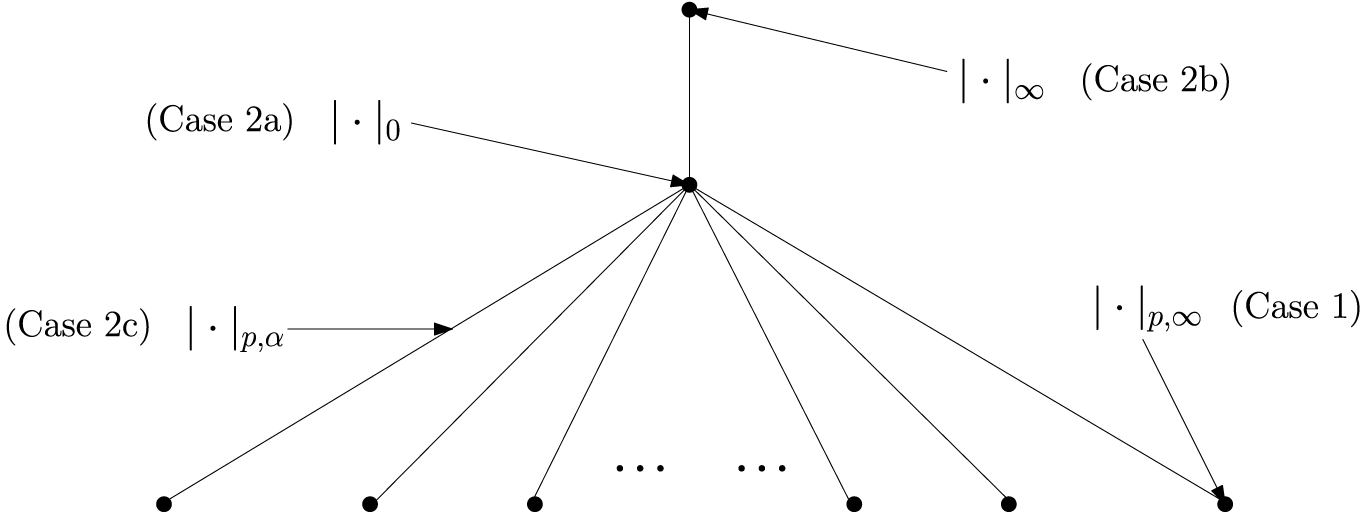
Assembling this data together, one obtains the picture in Figure 1.
$\mathcal {M}(\mathbb {Z})$
 .

Figure 1. Long description
A hierarchical tree diagram with nodes represented by black dots. At the top is a single node with an arrow pointing to it from the label absolute value sub infinity (Case 2b). A vertical line connects this top node to a central middle node. An arrow points to this middle node from the label absolute value sub 0 (Case 2a). From this middle node, seven lines fan out downward to a base row of nodes. On the far left of this fan, an arrow points to a line from the label absolute value sub p, alpha (Case 2c). The base row consists of seven visible nodes with ellipses in the center. On the far right of the base row, an arrow points to the final node from the label absolute value sub p, infinity (Case 1).
Example 1.36. Fix an algebraically-closed non-Archimedean field
$(K,|\cdot |)$
 . We define the Banach ring
$(\mathcal {A},||\cdot ||)$
 whereby:
-
• R is a non-negative real number.
-
• $\mathcal {A}$
is the ring of power series converging in radius R
(10) $$ \begin{align} \mathcal{A}=K\{R^{-1}T\}:=\left\{f=\displaystyle\sum_{i=0}^{\infty}c_i T^i\,\Bigg|\, c_i\in K, \displaystyle\lim_{i\rightarrow\infty}|c_i|R^i =0 \right\}. \end{align} $$
-
• $||\cdot ||$
is the so-called Gauss norm
(11) $$ \begin{align} ||f||:=\sup_i|c_i|R^i,\quad \text{where } f\in\mathcal{A}. \end{align} $$


The description of
$\mathcal {M}(\mathcal {A})$
 differs depending on whether K is trivially or non-trivially valued.
-
• Case 1: K is trivially valued. In which case,
(12) $$ \begin{align} K\{R^{-1}T\}=\begin{cases} K[[T]] \qquad \,\,\text{if}\, R<1 \\ K[T] \qquad\quad \text{if}\, R\geq 1, \end{cases} \end{align} $$
where $K[[T]]$
is the formal power series ring and
$K[T]$
is the polynomial ring.Footnote
21
When
$R<1$
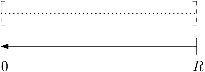
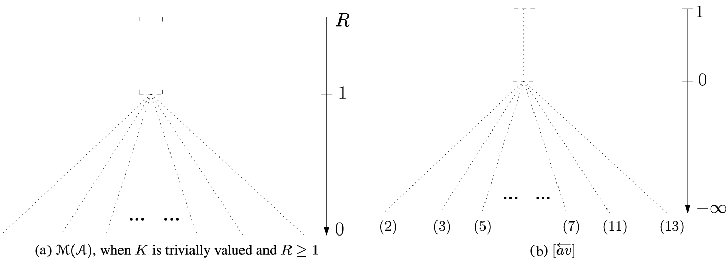
, one checks that the map
$|\cdot |_x\mapsto |T|_x$
yields a homeomorphism
$\mathcal {M}(\mathcal {A})\cong [0,R]$
; when
$R\geq 1$
,
$\mathcal {M}(\mathcal {A})$
has the structure of
$\mathcal {M}(\mathbb {Z})$
, as in Figure 1. For details, see [Reference Berkovich7, Example 1.4.4] or [Reference Jonsson22, Section 3.9.2]. -
• Case 2: K is non-trivially valued. In which case, $\mathcal {M}(\mathcal {A})$
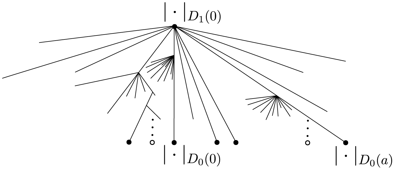
is a complicated tree with infinite branching points, as in Figure 2. Figure 2$\mathcal {M}(K\{R^{-1}T\})$
when
$R=1$
, adapted from [Reference Baker and Rumely3, Reference Silverman31].This follows from the following characterisation by Berkovich: all points of $x\in \mathcal {M}(\mathcal {A})$
can be realised as(13) $$ \begin{align} |\cdot|_x=\lim_{n\to\infty} |\cdot|_{D_{r_i}(k_i)} \end{align} $$
for some nested descending sequence of discs
(14) $$ \begin{align} D_{r_1}(k_1)\supseteq D_{r_2}(k_2)\supseteq\dots, \end{align} $$
where $|\cdot |_{D_{r}(k)}$
is a multiplicative seminorm canonically associated with the closed disc(15) $$ \begin{align} D_{r}(k):=\{b\in K \,\big| \, |b-k|\leq r\}. \end{align} $$
Discs of this form shall be referred to as a rigid disc. Notice this is analogous to the characterisation of $\mathbb {A}_{\mathrm {Berk}}^{1}$
in Summary Theorem 0.1 (ii).The reader may wonder: where did we use the hypothesis that K was non-trivially valued? Notice that the rigid discs in Equation (15) are defined as subsets of K. As such, in order for their radii to be well-defined (i.e., if $D_{r}(k)=D_{r'}(k')$
then
$r=r'$
) the base field K is forced to be non-trivially valued.Footnote
22
In fact, since
$|\cdot |_{D_{r}(k)}$
is defined by sending(16) $$ \begin{align} |f|_{D_{r}(k)}:=\sup_{z\in D_{r}(k)} |f(z)|, \end{align} $$these multiplicative seminorms begin to collapse into one another when K is trivially-valued, causing the original approximation argument to break down.


Remark 1.37. The Berkovich Affine Line
$\mathbb {A}_{\mathrm {Berk}}^1$
 is defined as the space of multiplicative seminorms on
$K[T]$
 . Is
$\mathbb {A}_{\mathrm {Berk}}^1$
 therefore just another example of a Berkovich spectrum? The answer, perhaps surprisingly, is generally no. Recall: Berkovich spectra are defined for Banach Rings. When K is non-trivially valued, one can check that
$K[T]$
 fails to be complete with respect to the Gauss norm
$||\sum a_iT^i||=\max _{i}|a_i|$
 . However, two important caveats:
-
(a) One can also check that $K\{R^{-1}T\}$
is in fact a Banach ring (with respect to the appropriate Gauss norm), and that
$\mathbb {A}_{\mathrm {Berk}}^1$
can be represented as an infinite union of Berkovich spectra$$\begin{align*}\mathbb{A}_{\mathrm{Berk}}^1\cong \bigcup_{R>0}\mathcal{M}(K\{R^{-1}T\}).\end{align*}$$
-
(b) When K is trivially valued, then $K[T]$
turns out to be complete with respect to
$||\cdot ||$
and thus defines a Banach ring; in which case, the two constructions do coincide. This gives another way of reading the difference between the trivially vs. non-trivially valued fields in the Berkovich setting.


For details, see, e.g., [Reference Berkovich7, Example 1.4.4] or [Reference Baker and Rumely3, Chapters 1–2].
Example 1.38. Extending Example 1.36, given
$R_1,\dots ,R_n>0$
 , define the ring

where
$|\mathsf {v}|=\mathsf {v}_1+\dots +\mathsf {v}_n$
 and
$R^{\mathsf {v}}=R_1^{\mathsf {v}_1}\dots R_n^{\mathsf {v}_n}$
 . To turn
$ K\{R_1^{-1}T_1,\dots , R_n^{-1}T_n\}$
 into a Banach ring, we equip it with the Gauss norm
$||\cdot ||$
 , where

When
$R_i=1$
 for all i, then
$K\{R_1^{-1}T_1,\dots , R_n^{-1}T_n\}$
 is called the Tate Algebra.
These Banach rings play an important role in Berkovich geometry because they allow us to define K-affinoid algebras, which arise as admissible quotients of these power series rings. More precisely, a K-affinoid algebra
$\mathcal {A}$
 is a commutative Banach ring for which there exists an admissible epimorphism

This should be understood as the analogues of quotients of polynomial rings in classical scheme theory; in particular, one constructs a Berkovich K-analytic space by gluing together the Berkovich spectra
$\mathcal {M}(\mathcal {A})$
 of these K-affinoid algebras. For a readable overview, see [Reference Baker and Rumely3, Sections C.4 and C.5].
2 Berkovich’s classification theorem, revisited
An organising theme of this section is the language of filters, which gives a transparent way of understanding how certain key notions in topology, logic, and non-Archimedean geometry interact. We motivate our study by way of a biased historical overview.
-
(1) On the side of geometry, the fact that the points of a Berkovich spectrumFootnote 23 $\mathcal {M}(\mathcal {A})$
may be characterised as ultrafilters was already known by the 1990s [Reference Berkovich7, Remark 2.5.21]. -
(2) On the side of logic, the fact that the (complete) types over a model may also be characterised as ultrafilters was well understood by the 1960s [Reference Morley24], if not earlier.

Yet it was only within the last 10 years that the two perspectives started to converge. Most notably, fixing a valued field K of rank 1, Hrushovski and Loeser [Reference Hrushovski and Loeser17, Section 14.1] showed that the Berkovich analytification of any quasi-projective variety V over K can be described using the language of definable types (cf. item (iii) of Summary Theorem 0.1). The power of the logical perspective may be measured by the fact that the authors were able to establish many deep results in non-Archimedean geometry (e.g., Theorem 1.32) that were inaccessible to previous methods (at least, without assuming, e.g., smoothness).
This sets up our present investigation. The understanding that models of a propositional geometric theory can be characterised as completely prime filters is well-known to topos theorists, although the connections with model-theoretic types appear to be under-developed (but see Discussion 1.22). In this section, we follow the model theorist’s cue and use point-free techniques to study the points of the Berkovich spectra
$\mathcal {M}(K\{R^{-1}T\})$
 from Example 1.36.
2.1 Berkovich’s disc theorem
We fix the following hypothesis for the rest of this section.
Hypothesis 2.1.
-
(i) K is an algebraically closed field, complete with respect to a non-Archimedean norm $|\cdot |$
, i.e.,$$ \begin{align*}|c_1+c_2|\leq\max\{|c_1|,|c_2|\} \qquad\text{for all}\, c_1,c_2\in K.\end{align*} $$
We emphasise that we allow $|\cdot |$
to be trivial (i.e.
$|\cdot |$
maps all non-zero
$c\in K$
to 1). -
(ii) Fix R to be any non-negative Dedekind real, and let $Q_+$
denote the set of positive rationals. -
(iii) Define $K_R:=\{k\in K \, |\, |k|\leq R \}$
. -
(iv) Following Example 1.36: define a Banach ring $(\mathcal {A},||\cdot ||)$
, where$$ \begin{align*}\mathcal{A}:=K\{R^{-1}T\}\end{align*} $$denotes the ring of power series converging on radius R, and $||\cdot ||$
is the associated Gauss norm.


Remark 2.2. A couple of orienting remarks:
-
• By [Reference Ng and Vickers27, Observation 0.1], the norm on K must be Dedekind-valued—this was shown to be a consequence of the field structure on K.
-
• Several results below—notably those concerning bounded K-seminorms on $\mathcal {A}_{\mathrm {Lin}}$
—only require that K be a non-Archimedean valued field, without completeness or being algebraically closed. We nevertheless adopt Hypothesis 2.1 as a standing assumption to streamline later comparisons with the classical Berkovich spectrum.

In order to classify the bounded multiplicative seminorms on
$\mathcal {A}$
 , we first reduce our study to something algebraically simpler.
Definition 2.3 (Bounded K-Seminorms).
-
(i) Define
(20) $$ \begin{align} \mathcal{A}_{\mathrm{Lin}}:=\{ aT-b \,|\, a,b \in K\}\cong K^2. \end{align} $$
Classically, $\mathcal {A}_{\mathrm {Lin}}$
is just a K-algebra, but we shall regard it as a point-free space in the sense of Section 1.1.1. Notice when we set
$a=0$
, we recover
$K\subset \mathcal {A}_{\mathrm {Lin}}$
. -
(ii) A K-seminorm on $\mathcal {A}_{\mathrm {Lin}}$
is an upper-valued map, which we denoteFootnote
24
(21) $$ \begin{align} |\cdot|_x\colon \mathcal{A}_{\mathrm{Lin}}\longrightarrow \overleftarrow{[0,\infty)} \end{align} $$satisfying the conditions:
-
• (Preserves constants). $|a|_x$
= the right Dedekind section of
$|a|$
; -
• (Semi-multiplicative). $|aT-b|_x=|a|\cdot |T-\frac {b}{a}|_x$
, for non-zero a; -
• (Ultrametric Inequality). $|f+f'|_x\leq \max \{|f|_x,|f'|_x\}$
;
for all $a\in K$
, and
$f,f'\in \mathcal {A}_{\mathrm {Lin}}$
. -
-
(iii) We define the Gauss Norm on $\mathcal {A}_{\mathrm {Lin}}$
as$$\begin{align*}||aT-b||:= \text{right Dedekind section of} \max\{|a|R, |b|\},\end{align*}$$where $aT-b\in \mathcal {A}_{\mathrm {Lin}}$
. A K-seminorm
$|\cdot |_x$
is called bounded if
$|\cdot |_x\leq ||\cdot ||$
.


Convention. For readability, we typically abuse notation and write, e.g., “
$|a|_x=|a|$
 ” instead of writing out “
$|a|_x$
 = the right Dedekind section of
$|a|$
 .” No constructive issue is hidden here, although sometimes we will perform certain computations at the Dedekind level before passing to the upper reals.
Remark 2.4. It is well-known [Reference Baker and Rumely3, Lemma 1.1] that any bounded multiplicative seminorm
$|\cdot |_x$
 satisfies
$|a|_x=|a|$
 and
$|f+g|_x\leq \max \{|f|_x,|g|_x\}$
 for any
$f,g\in \mathcal {A}$
 —this justifies the axioms in Definition 2.3(ii). Notice also that we did not require a K-seminorm to be multiplicative (only semi-multiplicative), but this is reasonable since
$\mathcal {A}_{\mathrm {Lin}}$
 is not closed under multiplication.
Reminder 2.5. To eliminate potential confusion:
-
• A multiplicative seminorm is defined on the whole ring $\mathcal {A}$
of convergent power series. -
• A K-seminorm, which is not multiplicative, is only defined on the space of linear polynomials $\mathcal {A}_{\mathrm {Lin}}$
.


We justify the reduction to linear polynomials in the following Preparation Lemma.
Lemma 2.6 (Preparation Lemma).
-
(i) Let K be any non-Archimedean field (not necessarily algebraically-closed or complete). Then, any bounded K-seminorm on $\mathcal {A}_{\mathrm {Lin}}$
is determined by its values on linear polynomials
$T-c$
, where
$c\in K_R$
. Moreover, this result satisfies geometricity (in the sense of Convention 1.13). -
(ii) Let $(\mathcal {B},||\cdot ||_{\mathcal {B}})$
be a Banach ring with a subring
$\mathcal {B}'\subseteq {\mathcal {B}}$
dense with respect to
$||\cdot ||_{{\mathcal {B}}}$
. Then, any bounded multiplicative seminorm on
$\mathcal {B}$
is determined by its values on
$\mathcal {B}'$
. -
(iii) Let K be as in Hypothesis 2.1. Then, any bounded multiplicative seminorm on $\mathcal {A}$
is determined by its values on linear polynomials
$T-c$
, where
$c\in K_R$
.


Proof. (i): We first give the proof, before explaining the connections to geometricity. The argument will require all parts of the definition of a bounded K-seminorm.
Consider a linear polynomial
$aT-b$
 . If
$a=0$
 , then

which agrees with the underlying field norm since K-seminorms preserve constants. If a is a unit, then semi-multiplicativity gives

Thus
$|\cdot |_x$
 is determined by its values on polynomials of the form
$T-c$
 , with
$c\in K$
 .
We now distinguish two cases.
-
• Case 1: $|c|\leq R$
. Then
$c\in K_R$
, so
$T-c$
already belongs to the distinguished family of linear polynomials in the Lemma’s statement. -
• Case 2: $R<|c|$
. Since
$0\leq R$
, this implies
$c\neq 0$
. By semi-multiplicativity,(22) $$ \begin{align} |T-c|_x=|c|\cdot |c^{-1} T - 1|_x. \end{align} $$
Because $|\cdot |_x$
is bounded by the Gauss norm, computeFootnote
25
(23) $$ \begin{align} |c^{-1} T|_x \leq ||c^{-1} T|| =|c|^{-1}\cdot R < 1 . \end{align} $$
We now apply the ultrametric inequality twice to show $|c^{-1}T-1|_x=1$
. First,(24) $$ \begin{align} |1|_x=\big|(c^{-1} T - 1) - c^{-1} T\big|_x\leq \max\big\{ |c^{-1} T - 1 |_x, |c^{-1} T|_x \big\}. \end{align} $$
Since $|c^{-1} T|_x<1$
(Equation (23)) and since
$|1|_x=1$
, it follows that(25) $$ \begin{align} 1\leq |c^{-1} T -1 |_x. \end{align} $$
Applying the ultrametric inequality once more gives
(26) $$ \begin{align} |c^{-1}T-1|_x \leq \max\{ |c^{-1} T |_x, 1\} = 1\, \end{align} $$and so
(27) $$ \begin{align} |c^{-1} T -1|_x = 1. \end{align} $$
Substituting this into Equation (22), we obtain
$$ \begin{align*}|T-c|_x= |c| \qquad\text{whenever \,\,} R<|c|.\end{align*} $$


At this point, the classical argument is complete. Since
$|T-c|_x=|c|$
 whenever
$R<|c|$
 (Case 2), we only need to know the values of
$|T-c|_x$
 for all
$c\in K_R$
 in order to determine its values on all of
$\mathcal {A}_{\mathrm {Lin}}$
 (Case 1). We now review our reasoning to check that we have in fact adhered to the constraints of geometricity.
Why does the result satisfy geometricity?
-
• Hypotheses. The structure of a non-Archimedean field K admits axiomatisation by geometric logic [Reference Ng and Vickers27, Section 2]. Moreover, the declaration “fix a non-negative Dedekind R” corresponds to working internally in the topos of sheaves over $[0,\infty )$
(see [Reference Ng and Vickers26, Convention 1.9]). -
• Proof. Although the case-splitting “ $|c|\leq R$
or
$R<|c|$
” resembles an appeal to excluded middle, it is justified geometrically since
$[0,R]$
and
$(R,\infty )$
are Boolean complements in the lattice of subspaces of
$[0,\infty )$
(see [Reference Ng and Vickers27, Discussion 4.10] or [Reference Vickers38, Theorem 1]). Similarly, the assumption that any
$a\in K$
is either 0 or a unit in K follows from an axiom in the geometric theory of fields [Reference Johnstone18, Section 2]. Finally, the argument makes use of standard arithmetic properties of multiplication on non-negative reals, which are justified in this setting; for the fine print, see [Reference Ng and Vickers26, Section 1.3].


(ii): Fix a bounded multiplicative seminorm
$|\cdot |_x$
 on
$\mathcal {B}$
 , and suppose
$f\in \mathcal {B}$
 . Consider any positive rational
$\epsilon>0$
 and any
$g\in \mathcal {B'}$
 such that
$||f-g||_{\mathcal {B}}<\epsilon $
 . Applying the ultrametric inequality and boundedness of
$|\cdot |_x$
 , compute:


Hence, if
$g\to f$
 with respect to
$||\cdot ||_{\mathcal {B}}$
 , then
$|g|_x\to |f|_x$
 . The claim then follows from
$\mathcal {B}'$
 being a dense subalgebra in
$\mathcal {B}$
 .
(iii): The following two basic observations get us almost all the way:
-
(a) The polynomial ring $K[T]$
is a dense subalgebra in
$\mathcal {A}$
, since any
$f\in \mathcal {A}$
can be expressed as$$\begin{align*}f=\sum_{i=0}^{\infty}a_iT^i = \lim_{n\to\infty}\sum^{n}_{i=0}a_i T^i, \qquad \text{where}\, |a_i|R^i\to 0.\end{align*}$$
-
(b) Since K is algebraically closed, any polynomial $g\in K[T]$
can be expressed as$$\begin{align*}g=c \prod^m_{j=1} (T-b_j),\end{align*}$$where $c,b_j\in K$
, for all
$1\leq j\leq m$
.


Applying item (ii) of the Lemma, Observations (a) and (b) together imply that any bounded multiplicative seminorm
$|\cdot |_x$
 on
$\mathcal {A}$
 is determined by its values on linear polynomials
$T-b$
 with
$b\in K$
 . The rest is analogous as in (i).
Remark on geometricity. Unlike item (ii), here we implicitly assume K is a complete field, a non-geometric property. Hence, the result (iii) should be regarded as classical (as opposed to satisfying geometricity).
Remark 2.7. For the reader familiar with non-Archimedean geometry, the proof of Preparation Lemma 2.6 mirrors, in a very simple setting, the underlying argument of the Weierstrass Preparation Theorem, which informally says: convergent power series often look like polynomials when restricted to a closed disc. Stated more precisely: all non-zero
$f\in \mathcal {A}$
 with finite order
$m\geq 0$
 can be represented as

where
$u(T)$
 is a unit power series on the closed disc
$K_R$
 , and W is a monic polynomial (the “Weierstrass polynomial”) with both degree and order m. However, unlike, e.g., [Reference Baker and Rumely3], we shall avoid invoking the Weierstrass Preparation Theorem since it only applies to non-zero
$f\in \mathcal {A}$
 with finite order. This would create issues when considering
$K\{R^{-1}T\}$
 with irrational radius R, which we can avoid with our approach.
We now introduce a special class of “filters” that highlights the topological structure of
$\mathcal {M}(\mathcal {A})$
 .
Definition 2.8 (Formal Non-Archimedean Balls).
A formal non-Archimedean ball is an element
$(k,q)\in K_R\times Q_{+}$
 . We represent this using the more suggestive notation
$B_q(k)$
 , to emphasise that we should view this pair as denoting a disc of radius q centred at k. In particular, we write

Observation 2.9. By decidabilityFootnote
26
of
$<$
 on
$Q_{+}$
 , one obtains the following sequents from the definition of
$\subseteq $
 from Definition 2.8:
-
(i) $|k-k'|<q\longrightarrow B_{q}(k')=B_{q}(k)$
. -
(ii) $B_{q}(k)=B_{q'}(k')\longrightarrow q=q'$


Discussion 2.10 (Rigid discs vs. Formal balls).
Notice item (ii) of Observation 2.9 says that the radii of the formal balls are well-defined (essentially by construction), even when the norm
$|\cdot |$
 on K is trivial. This should be contrasted with the classical rigid discs from Example 1.36

whose radii are well-defined only if
$|\cdot |$
 is non-trivial due to the point-set formulation.
Remark 2.11. The language of formal balls may strike the classical reader as a peculiar abstraction, but in fact they are sufficiently expressive to provide point-free accounts of standard completions of metric spaces [Reference Vickers33, Reference Vickers35]. Once the connection between the Berkovich construction and the completion of a space is made precise, these techniques can be adjusted accordingly to our present context.Footnote 27
Definition 2.12 (Filters of Formal Non-Archimedean Balls).
A filter of formal non-Archimedean balls
$\mathcal {F}$
 is an inhabitedFootnote
28
subset of
$K_R\times Q_{+}$
 satisfying the following conditions:
-
• (Upward closed with respect to $\subseteq $
). If
$B_{q'}(k')\subseteq B_{q}(k)$
and
$B_{q'}(k')\in \mathcal {F}$
, then
$B_{q}(k)\in \mathcal {F}$
. -
• (Closed under pairwise intersections). If $B_{q}(k),B_{q'}(k')\in \mathcal {F}$
, then there exists some
$B_{r}(j)\in \mathcal {F}$
such that
$B_r(j)\subseteq B_{q}(k)$
and
$B_r(j)\subseteq B_{q'}(k')$
.


Further, we call
$\mathcal {F}$
 an R-good filter if it also satisfies the following two conditions:
-
• For any $k\in K_R$
, and
$q\in Q_+$
such that
$R<q$
,
$B_{q}(k)\in \mathcal {F}$
. -
• If $B_{q}(k)\in \mathcal {F}$
, there exists
$B_{q'}(k')\in \mathcal {F}$
such that
$q'<q$
.


Convention 2.13. In this section, unless stated otherwise:


Observation 2.14 (Radius of R-Good Filters).
Let
$\mathcal {F}$
 be an R-good filter. Define the radius of
$\mathcal {F}$
 as

Then,
$\mathsf {rad}_{\mathcal {F}}$
 defines an upper real in
$\overleftarrow {[0,R]}$
 .
Proof. Roundedness and upward closure is immediate from the definition of
$\mathcal {F}$
 being an R-good filter, and so
$\mathsf {rad}_{\mathcal {F}}$
 defines an upper real. The fact that
$\mathsf {rad}_{\mathcal {F}}\in \overleftarrow {[0,R]}$
 follows from additionally noting:
-
• $\mathsf {rad}_{\mathcal {F}}$
is a subset of positive rationals. Hence,
$0\leq \mathsf {rad}_{\mathcal {F}}$
. -
• By $\mathcal {F}$
being R-good, we know
$q\in \mathsf {rad}_{\mathcal {F}}$
for all rationals
$q>R$
. Hence,
$\mathsf {rad}_{\mathcal {F}}\leq R$
.


Construction 2.15. Suppose we have a bounded K-seminorm
$|\cdot |_x$
 on
$\mathcal {A}_{\mathrm {Lin}}$
 . We then define the following collection of formal balls:

Claim 2.16.
$\mathcal {F}_x$
 is an R-good filter.
Proof. By Definition 2.12, we need to check that
$\mathcal {F}_x$
 is …
-
• …Upward closed. Suppose $B_{q'}(k')\subseteq B_{q}(k)$
and
$B_{q'}(k')\in \mathcal {F}_x$
. Unpacking definitions, this means
$|k-k'|<q$
and
$q'\leq q$
, as well as
$|T-k'|_x<q'$
. But since$$\begin{align*}\kern-8pt |T-k|_x = |(T-k') + (k'-k)|_x \leq \max\{|T-k'|_x,|k-k'|\}<\max\{q',q\}=q,\end{align*}$$
this implies $B_{q}(k)\in \mathcal {F}_x$
. -
• …Closed under Pairwise Intersection. We first claim $\mathcal {F}_x$
is totally ordered by
$\subseteq $
. Why? Given any
$B_{q}(k),B_{q'}(k')\in \mathcal {F}_x$
, we get
$|T-k|_x<q$
and
$|T-k'|_x<q'$
, and so$$\begin{align*}|k-k'|=|(T-k')-(T-k)|_x \leq \max\{|T-k'|_x,|T-k|_x\}<\max\{q',q\}.\end{align*}$$
By decidability of $<$
on
$Q_{+}$
, this means either
$B_{q}(k)\subseteq B_{q'}(k')$
or
$B_{q'}(k')\subseteq B_{q}(k)$
, as claimed. The fact that
$\mathcal {F}_x$
is closed under pairwise intersection follows immediately. -
• …R-good.
-
– Suppose $B_q(k)\in \mathcal {F}_x$
, and so
$|T-k|_x<q$
by definition. Since
$|\cdot|_x$
is valued in upper reals, there exists
$q'\in Q_{+}$
such that
$|T-k|_x<q'<q$
, and so
${B_{q'}(k)\in \mathcal {F}_x}$
. -
– Suppose $k\in K_R$
and
$q\in Q_{+}$
such that
$R<q$
. This gives$$\begin{align*}|T-k|_x\leq \max\{|T|_x,|k|\}\leq \max\{||T||,|k|\}= R<q,\end{align*}$$
since $k\in K_R$
implies
$|k|\leq R$
by definition, and
$|T|_x\leq ||T||=R$
. Hence,
$B_q(k)\in \mathcal {F}_x$
.
-
-
• …Inhabited. Immediate from R-goodness.


In the converse direction, we define the following.
Construction 2.17. For any formal non-Archimedean ball
$B_{q}(k)$
 , we define
$|\cdot |_{B_{q}(k)}$
 as follows:

More generally, given an R-good filter
$\mathcal {F}$
 , we define
$|\cdot |_{\mathcal {F}}$
 as

for any linear polynomial
$T-a\in \mathcal {A}_{\mathrm {Lin}}$
 .Footnote
29
Remark 2.18. Let
$f\in \mathcal {A}$
 such that f converges on a rigid disc
$D_r(k)$
 . By the maximum modulus principle in non-Archimedean analysis (see, e.g., [Reference Baker and Rumely3, p. 3]), one can express
$|\cdot |_{D_{r}(k)}$
 as

Notice that
$|T-a|_{D_q(k)}$
 is classically equivalent to
$|T-a|_{B_q(k)}$
 just in case
$r=q$
 . Nonetheless, the definition of
$|\cdot |_{D_{r}(k)}$
 as stated is problematic in our setting for two reasons:
-
(a) First, the use of $\sup $
presents a constructive issue. A
$\sup $
of Dedekinds yields a lower real (see Fact 1.21), whereas our K-seminorms are valued in upper reals, and there is no constructive way to switch between lower and upper reals.Footnote
30
On the other hand,
$\max $
and
$\mathrm {inf}$
are well-defined on the upper reals, which explains the formulation of Construction 2.17. -
(b) The rigid discs featured in Equation (29) are required to have bounded radius $0<r\leq R$
, which ensures the convergence of
$|f|_{D_{r}(k)}$
for any
$f\in \mathcal {A}$
. On the other hand, the radius of the formal balls
$B_{q}(k)$
have no upper bound. Nonetheless, we avoid convergence issues since
$|\cdot |_{B_q(k)}$
is restricted to just the linear polynomials.


Having established Construction 2.17, we perform the obligatory check.
Claim 2.19.
$|\cdot |_{\mathcal {F}}$
 determines a bounded K-seminorm on
$\mathcal {A}_{\mathrm {Lin}}$
 . More explicitly, for any
$B_{q}(k)\in \mathcal {F}$
 , define

Then,

defines a bounded K-seminorm on
$\mathcal {A}_{\mathrm {Lin}}$
 that uniquely extends Construction 2.17.
Proof of Claim.
We first check that Equation (31) satisfies the required properties, before showing it gives the unique extension of
$|\cdot |_{\mathcal {F}}$
 .
-
• $|\cdot |_{\mathcal {F}}$
is valued in the upper reals, since
$|f|_{\mathcal {F}}$
takes the infimum of a set of Dedekinds. -
• To verify $|\cdot |_{\mathcal {F}}$
satisfies the properties listed in Definition 2.3(ii), one first verifies their obvious analogues for
$|\cdot |_{B_q(k)}$
, before observing that they are preserved by taking
$\mathrm {inf}$
’s.For instance, to show the ultrametric inequality, suppose we have $aT-b,a'T-b'\in \mathcal {A}_{\mathrm {Lin}}$
. Then, given any
$B_{q}(k)\in \mathcal {F}$
, compute(32) $$ \begin{align} |aT - b + a'T - b'|_{B_q(k)} &= \max\{|(a+a')k-(b+b')|,\, |a+a'|\cdot q\} \nonumber \\ &\leq \max\left\{ \max\{|ak-b|,|a'k-b'|\},\right. \nonumber\\ &\qquad\qquad \left. \max\{|a|\cdot q,|a'|\cdot q\}\right\} \nonumber\\ &= \max\{|aT-b|_{B_{q}(k)},|a'T-b'|_{B_q(k)}\}, \end{align} $$
where the middle inequality is by the ultrametric inequality satisfied by the original norm $|\cdot |$
on K. Since this inequality holds for all
$B_{q}(k)\in \mathcal {F}$
, taking the infimum on both sides of inequality in Equation (32) over all
$B_{q}(k)\in \mathcal {F}$
gives the desired ultrametric inequality for
$|\cdot |_{\mathcal {F}}$
(33) $$ \begin{align} |aT - b + a'T - b'|_{\mathcal{F}} \leq \max\{|aT-b|_{\mathcal{F}},\, |a'T-b'|_{\mathcal{F}}\}. \end{align} $$
Similarly, semi-multiplicativity follows from checking that $|aT-b|_{B_{q}(k)} = |a|\cdot |T-b/a|_{B_q(k)}$
for
$a\neq 0$
, which is preserved under taking infima. -
• We now check boundedness. For any R-good filter $\mathcal {F}$
,(34) $$ \begin{align} |T-a|_{\mathcal{F}}= \!\underset{B_{q}(k)\in \mathcal{F}}{\mathrm{inf}}\max\{|k-a|,q\}\leq \!\underset{B_{q}(k)\in \mathcal{F}}{\mathrm{inf}}\max\{|a|, |k|, q\}\leq \max\{|a|,R\}, \end{align} $$
where the final inequality is by R-goodness of $\mathcal {F}$
plus the fact that
$k\in K_R$
. The same argument extends to show that
$|aT-b|_{\mathcal {F}}\leq \max \{|a|\cdot R,|b|\}$
. Hence, conclude that
$|\cdot |_{\mathcal {F}}$
is bounded by the Gauss norm
$||\cdot ||$
.


It remains to show this defines the unique extension of the original
$|\cdot |_{\mathcal {F}}$
 . It is clear Equation (30) recovers the original
$|\cdot |_{B_q(k)}$
 in Construction 2.17 when restricted to
$T-b$
 or b. The only non-trivial case to check is
$aT-b$
 when a is non-zero. But semi-multiplicativity requires that

exactly as we defined in the Claim’s statement. The same holds for
$|\cdot |_{\mathcal {F}}$
 when we pass to
$\mathrm {inf}$
 ’s.
Finally, we remark that our present argument satisfies geometricity—the only potential subtlety is the case-splitting of when a is 0 or a unit, but this follows from the axioms of the geometric theory of fields (as already mentioned in the proof of Preparation Lemma 2.6 (i)).
As the reader may have anticipated, the algebraic constructions (i.e., bounded multiplicative seminorms and K-seminorms) and the topological constructions (i.e., the R-good filters) defined in this section have a close connection. This is made precise in the following two theorems, which together show that these constructions define equivalent spaces in a suitable sense.
On a first reading, the reader may safely interpret the proofs as establishing a bijection between the underlying sets of objects, postponing questions of topology to a later stage. To motivate the first theorem, note that the definitions of R-good filters and K-seminorms make sense for any non-Archimedean field—not necessarily algebraically-closed or complete. This leads to the following general result.
Theorem 2.20. Suppose K is a non-Archimedean valued field, and let

denote the usual space of linear polynomials. Then, the point-free space of bounded K-seminorms on
$\mathcal {A}_{\mathrm {Lin}}$
 is equivalent to the point-free space of R-good filters.
Proof. We start by showing Constructions 2.15 and 2.17 are inverse to each other, before explaining why this lifts to an equivalence of spaces. There are two main directions to check.
First Direction:
$|\cdot |_x=|\cdot |_{\mathcal {F}_{x}}$
.

Fix a bounded K-seminorm
$|\cdot |_x$
 . By Preparation Lemma 2.6 (i), it suffices to check that
$|\cdot |_x$
 and
$|\cdot |_{\mathcal {F}_x}$
 agree on linear polynomials
$T-a$
 such that
$a\in K_R$
 .
Suppose
$|T-a|_x<q$
 for some
$q\in Q_{+}$
 . Then,
$B_{q}(a)\in \mathcal {F}_x$
 by construction. In particular, there exists
$q'\in Q_+$
 such that

since
$|T-a|_x$
 defines an upper real. Further, since

and since Equation (35) implies
$B_{q'}(a)\in \mathcal {F}_x$
 , deduce that

and so

Conversely, suppose
$|T-a|_{\mathcal {F}_x}<q$
 for some
$q\in Q_{+}$
 . Since
$|T-a|_{\mathcal {F}_x}$
 defines an upper real, deduce there exists
$B_{q'}(k)\in \mathcal {F}_x$
 such that

By definition,
$B_{q'}(k)\in \mathcal {F}_{x}$
 implies
$|T-k|_x<q'$
 , and so

which in turn implies

Put together, Equations (37) and (38) give
$|\cdot |_x=|\cdot |_{\mathcal {F}_x}$
 , as claimed.
Second Direction:
$\mathcal {F}=\mathcal {F}_{|\cdot |_{\mathcal {F}}}$
.

Fix an R-good filter
$\mathcal {F}$
 . Suppose
$B_{q}(k)\in \mathcal {F}$
 . Since the radius
$\mathsf {rad}_{\mathcal {F}}$
 of
$\mathcal {F}$
 defines an upper real, there exists
$B_{q'}(k')\in \mathcal {F}$
 such that
$\mathsf {rad}_{\mathcal {F}}<q'<q$
 . Without loss of generality, we may assume
$k=k'$
 .Footnote
31
Since
$|T-k|_{B_{q'}(k)}=q'$
 , deduce that

In particular, this implies
$B_{q}(k)\in \mathcal {F}_{|\cdot |_{\mathcal {F}}}$
 , and so

Conversely, suppose
$B_{q}(k)\in \mathcal {F}_{|\cdot |_{\mathcal {F}}}$
 . Unpacking definitions, deduce there exists
$B_{q'}(j)\in \mathcal {F}$
 such that

To show that
$B_{q'}(j)\subseteq B_{q}(k)$
 , we need to show that
$|k-j|<q$
 and
$q'\leq q$
 . But this is clear from Equation (40). Since
$B_{q'}(j)\in \mathcal {F}$
 and
$\mathcal {F}$
 is upward closed, conclude that
$B_{q}(k)\in \mathcal {F}$
 , and so

Combining Equations (39) and (41) gives
$\mathcal {F}=\mathcal {F}_{|\cdot |_{\mathcal {F}}}$
 , as claimed.
Finish.
Thus far, we have only shown that Constructions 2.15 and 2.17 are inverse. To see why this lifts to an equivalence of spaces requires an appreciation of the connections to logic.
Definitions 2.3 and 2.12 implicitly present two (predicate) geometric theories, whose models are precisely the bounded K-seminorms on
$\mathcal {A}_{\mathrm {Lin}}$
 and R-good filters, respectively. The constructions above also satisfy geometricity in the sense of Remark 1.12, and our present argument shows they are mutually inverse on the generic models. Hence, by Criterion
$(\dagger )$
 in Remark 1.12, conclude that the corresponding point-free spaces are equivalent, as claimed.
For the next theorem, we will temporarily treat K-seminorms as taking values in Dedekind reals, rather than merely upper reals. Classically, this is a harmless identification since, in this setting, any bounded non-empty upper real uniquely determines a Dedekind real. Constructively, however, the two notions are inequivalent (as already alluded to in Fact 1.21); we shall return to this issue later.
Theorem 2.21. Assume Hypothesis 2.1. Let
-
• $\mathcal {M}(\mathcal {A})$
as the classical Berkovich spectrum, i.e., the space of Dedekind-valued multiplicative seminorm on
${\mathcal {A}}$
; -
• $\overleftarrow {\mathcal {M}(\mathcal {A}_{\mathrm {Lin}})}$
denote the space of bounded K-seminorms on
$\mathcal {A}_{\mathrm {Lin}}$
.


Then,
-
(i) Each $|\cdot |_x\in \mathcal {M}(\mathcal {A})$
is uniquely represented by an R-good filter. -
(ii) Classically, $\mathcal {M}(\mathcal {A})$
is equivalent to
$\overleftarrow {\mathcal {M}(\mathcal {A}_{\mathrm {Lin}})}$
. In particular,
$\mathcal {M}({\mathcal {A}})$
is classically equivalent to the space of R-good filters.


Proof. Let
$|\cdot |_x\in \mathcal {M}(\mathcal {A})$
 . Restricting
$|\cdot |_x$
 to linear polynomials defines a bounded K-seminorm

By Fact 1.21, the map
$x\mapsto R_x$
 sending a Dedekind to its right Dedekind section is monic. Consequently, (i) follows immediately from Preparation Lemma 2.6 and Theorem 2.20.
We now prove (ii). Throughout the remainder of the proof we make the following classical assumption:
-
(⋆) Any upper real $\gamma _U$
besides
$\pm \infty $
is canonically identified with a Dedekind real
$\gamma $
whose right Dedekind section is
$\gamma _U$
, and similarly for (bounded, non-empty) lower reals.


In the forward direction, following Equation (42), the restriction map

defines a map
$\mathcal {M}(\mathcal {A}) \to \overleftarrow {\mathcal {M}(\mathcal {A}_{\mathrm {Lin}})}$
 .
Conversely, by Theorem 2.20, any bounded K-seminorm on
$\mathcal {A}_{\mathrm {Lin}}$
 is of the form
$|\cdot |_{\mathcal {F}}$
 for a unique R-good filter
$\mathcal {F}$
 . We extend
$|\cdot |_{\mathcal {F}}$
 to a multiplicative seminorm on
$\mathcal {A}$
 in two stages.
Step 1: Polynomials.
Any polynomial
$f\in K[T]$
 admits a factorisation

Define

(As we later verify in Claim A.1. this defines a bounded multiplicative seminorm on
$K[T]$
 .)
Step 2: Power series.
Every power series
$f\in \mathcal {A}$
 can be written as limit of polynomials

Define

A few orienting remarks:
-
(a) Assumption $(\star )$
is used implicitly throughout, for instance to interpret
$|\cdot |_{\mathcal {F}}$
as Dedekind-valued in Equation (44), and to make sense of the limit in Equation (45). The existence and nature of this limit will be justified in the proof of Claim A.2. -
(b) Under $(\star )$
, item (i) strengthens to yield a subspace inclusion
$\mathcal {M}(\mathcal {A}) \hookrightarrow \overleftarrow {\mathcal {M}(\mathcal {A}_{\mathrm {Lin}})}$
. -
(c) Suppose the construction $\widetilde {|\cdot |_{\mathcal {F}}}$
defines a bounded multiplicative seminorm on
$\mathcal {A}$
. It is then straightforward to check that the constructions
$|\cdot |_x^{\mathrm {lin}}$
and
$|\cdot |_{\mathcal {F}}$
are inverse to each other. The identity(46) $$ \begin{align} |\cdot|_{\mathcal{F}} = \widetilde{|\cdot|_{\mathcal{F}}}^{\mathrm{lin}} \end{align} $$is immediate by construction, whereas the identity
(47) $$ \begin{align} |\cdot|_x= \widetilde{|\cdot|^{\mathrm{lin}}_x} \end{align} $$follows from Preparation Lemma 2.6 and checking the values on the linear polynomials.


As such, in order to prove the (classical) equivalence stated in the Theorem, it remains to verify that
$\widetilde {|\cdot |_{\mathcal {F}}}$
 is in fact a bounded multiplicative seminorm on
$\mathcal {A}$
 . The check relies on standard arguments from non-Archimedean analysis; details are given in Appendix A.
We conclude with some discussions on various aspects of the proof.
Discussion 2.22. Let us sketch the original argument from classical Berkovich geometry.
-
• Given any rigid disc $D_{r}(k)$
such that
$0<r\leq R$
, define a multiplicative seminorm
$ |\cdot |_{D_{r}(k)}$
on
$\mathcal {A}$
. -
• Next, given any nested sequence of discs $\mathsf {D}:= D_{r_1}(k_1)\supseteq D_{r_2}(k_2)\supseteq \dots $
, define the multiplicative seminorm
$|\cdot |_{\mathsf {D}}:=\mathrm {inf}_{\mathsf {D}} |\cdot |_{D_{r_i}(k_i)}$
. -
• Finally, given $|\cdot |_x\in \mathcal {M}(\mathcal {A})$
, define the nested sequence
$\mathsf {D}_{x}:=\{D_{|T-k|_x}(k)\,|\, k\in K \, \text {and}\, |k|\leq R\}$
. Check that
$|\cdot |_x$
and
$|\cdot |_{\mathsf {D}_x}$
agree on linear polynomials, and conclude
$|\cdot |_x=|\cdot |_{\mathsf {D}_x}$
.


The parallels with the proof for Theorem 2.20 are clear. However, the argument must be adjusted and finitised appropriately in order to work in our context. Some important differences:
-
(i) “Rational” discs. Both R-good filters and the nested sequence of discs $\mathsf {D}_x$
give rise to approximation arguments, but their approximants differ in important ways. In particular, whereas the radius of a formal ball
$B_{q}(k)$
is rational in the usual sense that
$q\in Q_{+}$
is a positive rational number, in non-Archimedean geometry a rigid disc
$D_r(k)\in \mathsf {D}_x$
is said to have rational radius when$$\begin{align*}r\in\Gamma:=\{|k|\in [0,\infty) \,|\, k\in K\},\end{align*}$$
i.e., r belongs to the value group of K. The terminology is standard, and indicates an analogy between $Q_{+}$
and
$\Gamma $
, but it is important to remember that they are not the same—particularly when K is trivially-valued. -
(ii) K-seminorms. Whereas the original argument starts by defining a multiplicative seminorm on $\mathcal {A}$
, before restricting it to the linear polynomials to perform certain checks, we instead defined a new algebraic structure (which we call K-seminorms) on the space of linear polynomials
$\mathcal {A}_{\mathrm {Lin}}$
. -
(iii) Use of filters. While Berkovich’s original argument shows that every $|\cdot |_x\in \mathcal {M}(\mathcal {A})$
corresponds to a nested descending sequence of discs, this representation is not unique. In particular, two different sequences of discs may define the same multiplicative seminorm on
$\mathcal {A}$
. We resolve this issue by appealing to the more natural language of filters, which allows us to obtain a representation result: every
$|\cdot |_x\in \mathcal {M}(\mathcal {A})$
is uniquely associated with an R-good filter
$\mathcal {F}_x$
. -
(iv) Use of formal balls. As already pointed out in Discussion 2.10, our result holds for both trivially and non-trivially valued K. This is in contrast to the original argument, which only works for non-trivially valued K.


Items (i) and (ii) reflect our decision to work with the upper reals as opposed to the Dedekinds, and strike a careful balance: whilst the upper reals are particularly suited to analysing the filters of formal balls (cf. Observation 2.14), they also impose strong (constructive) restrictions on the algebra (cf. Remark 2.18, but see also Discussion 2.23). Items (iii) and (iv) give evidence that filters (as opposed to nested sequences of discs) and formal balls (as opposed to the classical rigid discs) are the correct language for studying
$\mathcal {M}(\mathcal {A})$
 .
Finally, for the reader interested in constructive mathematics, we sort out and summarise the classical vs. constructive aspects of our result.
Discussion 2.23 (On Assumption
$(\star )$
).

Theorem 2.21 is classical because its proof relies on Assumption
$(\star )$
 , namely, that any bounded upper (or lower) real admits a canonical extension to a Dedekind real. Some natural points of discussion:
-
(i) Why is Assumption $(\star )$
classical? Consider the obvious argument: given an upper real R defined as the set of rationals strictly greater than 1, we define a lower real L as the set of rationals strictly less than 1. Hence, conclude that
$(L,R)$
is the Dedekind real canonically associated with R.This argument will strike most as reasonable, so where does it fail constructively? Discussion 1.25 reminds us that an upper real is blind to the rationals less than itself, suggesting it may only have the same knowledge as a Dedekind real by way of classical reasoning. Reformulated more precisely, we claim that if any upper real R can be associated with a lower real L such that $(L,R)$
defines a Dedekind real, then every proposition p has a Boolean complement
$p'$
—which holds classically, but not constructively (cf. Remark 1.4).To prove our claim, let p be any proposition, and define the subset of rationals:
$$\begin{align*}R:=\{ q\in\mathbb{Q} \,|\, \text{either } "q>1\text{" }or\ "p \text{ holds and } q>0\text{"}\}.\end{align*}$$
In other words, R is a kind of schizophrenic upper real: since p holds if and only if $R<1$
, R may define the upper real
$1$
or the upper real
$0$
, depending on the truth value of p. Now, suppose we have some lower real L such that
$(L,R)$
is Dedekind. Define a new proposition
$p' \leftrightarrow \frac {1}{2}<L$
. If
$(L,R)$
indeed define a Dedekind, one deduces-
(a) $\top \to p\vee p'$
;[Why? Locatedness of $(L,R)$
gives
$\frac {1}{2}<L\vee R<1$
.] -
(b) $p\land p'\to \bot $
.[Why? Since $p\to R<\frac {1}{2}$
, this gives
$p\land p'\to (\frac {1}{2}<L)\land (R<\frac {1}{2})$
, contradicting separatedness of
$(L,R)$
.]
This shows $p'$
is a Boolean complement of p, as claimed. -
-
(ii) Is Assumption $(\star )$
necessary? One might hope to constructivise Theorem 2.21 by replacing Dedekind-valued seminorms on
${\mathcal {A}}$
with upper-valued ones. However, our current proof proceeds by extending a multiplicative seminorm on
$K[T]$
to
${\mathcal {A}}$
by taking limits, a step which does not interact well with upper reals constructively (cf. Remark 2.18). It is not clear how to modify this argument without relying on Assumption
$(\star )$
. In any case,
$(\star )$
is unavoidable if one wishes to recover the classical Berkovich spectrum.


Summary 2.24 (Classical vs. Geometric Mathematics).
In the discussion below, the term “geometric” is used in the sense of geometric mathematics, i.e., a specific regime of constructive mathematics natural in point-free topology, dealing with constructions arising from colimits and finite limits (cf. Remark 1.12). Since our present work is influenced by point-free ideas, the question arises: to what extent do the results of this section adhere to these constraints?
-
(i) Theorem 2.20 is a fully geometric result. We only require K to be a non-Archimedean field, a structure which can be expressed geometrically. The only potential subtlety is our use of Preparation Lemma 2.6 in the proof; however, we only invoke item (i) of the Lemma, which satisfies geometricity.
-
(ii) Theorem 2.21 is both non-constructive and non-geometric on several levels. As already mentioned in Discussion 2.23, it invokes Assumption ( $\star $
), which is classical since it implies the LEM.Footnote
32
In addition, it assumes Hypothesis 2.1, which requires K to be a complete field, a non-geometric property. Moreover, as pointed out by Johnstone [Reference Johnstone18, Section 2], any non-trivial ring R satisfying the geometric formulation of the field axiom$$ \begin{align*}"\,\forall a\in R .\,\,a=0 \,\,\text{or}\,\, a\,\,\text{is a unit}\text{"},\end{align*} $$
must be decidable, and thus a discrete field. In other words, adhering to geometric mathematics would rule out many (topological) fields of interest in Berkovich geometry, e.g., the p-adic complex numbers $\mathbb {C}_p$
—which is certainly against the spirit of the theorem. -
(iii) Theorem 2.20 can be read as extracting the geometric content of Theorem 2.21. However, as presently stated, Theorem 2.20’s connections to Berkovich spectra are somewhat indirect, not least because of the geometricity issues underlying Hypothesis 2.1. Can we do any better?
Discussion 2.23 already pointed out the difficulties in removing Assumption $(\star )$
from Theorem 2.21. Moreover, although the polynomial ring
$K[T]$
and
$\mathcal {A}_{\mathrm {Lin}}$
can be defined geometrically for any field K, it is presently unclear how to do the same for the convergent power series ring
$K\{R^{-1}T\}$
.Footnote
33
In other words, in the context of geometric mathematics, even defining “multiplicative seminorm on
${\mathcal {A}}$
” is a challenge. Alternatively, one may wish to modify the definition of a K-seminorm to be Dedekind-valued, but this creates new issues for Theorem 2.20. In particular,
$|\cdot |_{\mathcal {F}}$
from Construction 2.17 is defined by taking
$\mathrm {inf}$
’s and so, at least constructively,
$|\cdot |_{\mathcal {F}}$
has to be upper-valued (cf. Fact 1.21).


2.2 Applications to the trivial case
As a slick application of Theorem 2.21, we recover the familiar characterisations of
$\mathcal {M}(\mathcal {A})$
 when K is trivially valued (see Example 1.36). What’s new here? For one, the proofs proceed differently from the standard arguments [Reference Berkovich7, Reference Jonsson22], which (unlike Theorem 2.21) treat the trivially and non-trivially valued cases separately. More fundamentally, our proofs give a very interesting indication of how Berkovich’s characterisation of
$\mathcal {M}(\mathcal {A})$
 (via nested sequences of discs) is in fact more robust than previously thought.
Example 2.25 (Case:
$R<1$
).

If
$R<1$
 and K is trivially valued, then
$K_R=\{0\}$
 . The R-good filters are thus entirely determined by their radii, and so the space of R-good filters is equivalent to
$\overleftarrow {[0,R]}$
 (see Observation 2.14). Applying Theorem 2.21, one deduces that
$\mathcal {M}(\mathcal {A})$
 is classically equivalent to
$\overleftarrow {[0,R]}$
 , essentially for free.
$\mathcal {M}(\mathcal {A})$
 , when K is trivially valued and
$R<1$
 .

Example 2.26 (Case:
$R\geq 1$
).

If
$R\geq 1$
 and K is trivially valued, then notice
$K_R=K$
 . Consider the following two subcases:
-
Subcase 1: $\mathcal {F}$
is an R-good filter with radius
$\mathsf {rad}_{\mathcal {F}}\geq 1$
. In which case:-
(a) $B_{q}(k)\in \mathcal {F}$
for any
$k\in K$
and any
$q>\mathsf {rad}_{\mathcal {F}}$
.[Why? Since $\mathcal {F}$
is R-good, there must exist some
$B_{q}(k')\in \mathcal {F}$
for any
$q>\mathsf {rad}_{\mathcal {F}}$
. Since K is trivially valued, we get
$|k-k'|\leq 1 \leq \mathsf {rad}_{\mathcal {F}} < q$
for any
$k\in K$
, and so
$B_{q}(k')= B_{q}(k)$
.] -
(b) The space of such R-good filters form an interval $\overleftarrow {[1,R]}$
.[Why? Immediate from (a), which shows any R-good filter with $\mathsf {rad}_{\mathcal {F}}\geq 1$
is entirely determined by its radius.]
-
-
Subcase 2: $\mathcal {F}$
is an R-good filter with radius
$\mathsf {rad}_{\mathcal {F}}<1$
. In which case:-
(a) If $B_q(k)$
such that
$q>1$
, then
$B_{q}(k)\in \mathcal {F}$
.[Why? Since $\mathsf {rad}_{\mathcal {F}}<1$
, there exists some
$k'\in K$
such that
$B_{1}(k')\in \mathcal {F}$
. Since K is trivially valued, deduce that
$B_{1}(k')\subseteq B_{q}(k)$
and so
$B_{q}(k)\in \mathcal {F}$
since
$\mathcal {F}$
is upward closed.] -
(b) If $B_{q}(k)\in \mathcal {F}$
and
$q\leq 1$
, then
$k=k'$
for any
$B_{q'}(k')\in \mathcal {F}$
such that
${q'\leq 1}$
.[Why? Take the “pairwise intersection” of $B_q(k),B_{q'}(k')\in \mathcal {F}$
to get
$B_{q"}(k")\in \mathcal {F}$
. Since
$B_{q"}(k")\subseteq B_{q}(k)$
, this forces
$k"=k$
since otherwise
$1=|k"-k|< q\leq 1$
, contradiction. The same argument shows that
$k"=k'$
, and so we conclude
$k'=k$
.]
-


Summarising, an R-good filter
$\mathcal {F}$
 with radius
$\mathsf {rad}_{\mathcal {F}}\geq 1$
 is entirely determined by its radius (Subcase 1), whereas an R-good filter
$\mathcal {F}$
 with
$\mathsf {rad}_{\mathcal {F}}< 1$
 is determined by its radius plus its unique choice of
$k\in K$
 (Subcase 2). Applying Theorem 2.21 once more, deduce that the space
$\mathcal {M}({\mathcal {A}})$
 has the structure depicted in Figure 4.
(a)
$\mathcal {M}(\mathcal {A})$
 , when K is trivially valued and
$R\geq 1$
 . (b)
$[ \overleftarrow {av}]$
 .

Figure 4. Long description
Panel a shows a tree structure with a single vertical dotted line at the top, enclosed in dashed brackets, which then branches out into six dotted lines spreading downward. Between the central branches are two sets of three dots indicating continuation. To the right is a vertical axis with an arrow pointing down. The axis is labeled R at the top, 1 in the middle, and 0 at the bottom arrow tip.
Panel b shows a similar tree structure. A vertical dotted line at the top branches into seven dotted lines spreading downward. The base of these lines are labeled from left to right with numbers in parentheses: 2, 3, 5, followed by two sets of three dots, then 7, 11, and 13. To the right is a vertical axis with an arrow pointing down. The axis is labeled 1 at the top, 0 in the middle, and negative infinity at the bottom arrow tip.
This should be compared with
$[\overleftarrow {av}]$
 , the space of multiplicative seminorms on
$\mathbb {Z}$
 defined in [Reference Ng and Vickers27], shown in Figure 4. Notice the two spaces have the same structure, up to a
$\log _R\text {(---)}$
 transformation.


3 An algebraic fork in the road
Let us review our work. In principle, the extension of Berkovich’s original result to Theorem 2.21 could have been discovered much earlier. And yet it was not—to our knowledge, the idea that one could modify the language of rigid discs to classify the points of
$\mathcal {M}(K\{R^{-1}T\})$
 without requiring K to be non-trivially valued was not suspected by the experts.Footnote
34
The reason for this seems to be that Theorem 2.21, both in its formulation and proof, belongs to the point-free perspective in an essential way. Of course, one certainly does not need to be a topos theorist in order to, e.g. understand what a formal ball is, but there are specific intuitions from the point-free perspective that guided us to our result:
-
(a) Topos theory encourages one to investigate how the same idea may be expressed in different settings, and to ask about the connections.Footnote 35 In particular, recall: any essentially propositional theory corresponds to a space of completely prime filters. Work in [Reference Ng and Vickers27] showed that the theory of multiplicative seminorms on $\mathbb {Z}$
is essentially propositional. Given the obvious parallels between
$\mathcal {M}(\mathbb {Z})$
and
$\mathcal {M}(K\{R^{-1}T\})$
when K is trivially normed and
$R\geq 1$
(cf. Example 2.26), the topos theorist may guess that
$\mathcal {M}(K\{R^{-1}T\})$
also admits a meaningful description via completely prime filters. -
(b) Once we defined the formal ball $B_{q}(k)$
and the correct inclusion relation
$B_{q'}(k')\subseteq B_{q}(k)$
, the rest of the argument began to fall into place. But notice: the decision to use formal balls (as opposed to the classical rigid discs) reflects the localic perspective that it is the opens that are the basic units for defining a space, and not the underlying set of points. Compare, for instance, our use of formal balls with the symbols
$P_{qr}$
in the propositional theory of Dedekinds
$\mathbb {T}_{\mathbb {R}}$
(cf. Discussion 1.15).


Though Theorem 2.21 is relatively straightforward, its more surprising features point to the clarifying potential of point-free methods in addressing foundational questions in non-Archimedean geometry. Motivated by this, we conclude with a list of inter-related problems aimed at exploring this potential further.
3.1 Trivially vs. non-trivially valued fields
First, an obvious piece of mathematical due diligence. Many results in Berkovich geometry are sensitive to the case-split between trivially vs. non-trivially valued (non-Archimedean) fields. This motivates the following general exercise.
Problem 3.1. Pick an interesting result in Berkovich geometry that appears to rely on the base field K being non-trivially valued. Examine why. Just as in Theorem 2.21, can we eliminate this hypothesis by applying point-free techniques? If yes, what applications does this generalised result give us?
Discussion 3.2. Here’s one place to start looking. In non-Archimedean geometry, a common strategy for proving results on an irrational (or open) disc
$\mathsf {D}$
 is to first prove the result for rational closed discs, before extending the result to
$\mathsf {D}$
 by expressing it as a nested union of rational closed discs (see, e.g. [Reference Benedetto4]). This strategy obviously breaks down when K is trivially valued, but the language of upper reals may offer a workaround (cf. Discussion 2.22).
3.2 Overconvergent lattices and rigid geometry
We now discuss a more solid lead. In unpublished work of Dudzik [Reference Dudzik11] as well as Baker’s Berkeley Lecture Notes [Reference Baker1], the following notion was defined.
Definition 3.3. Consider a lower-bound distributive lattice L, with finite
$\land $
 and
$\vee $
 and a minimal element denoted
$\bot $
 .
-
(i) For $x,x'\in L$
, we say x is inner in
$x'$
, written
$x\triangleleft x'$
, if for all
$z\geq x'$
, there exists w with
$x\land w = \bot $
and
$x'\vee w=z$
. -
(ii) We call L an overconvergent lattice if for all $x,y\in L$
, where
$x\land y=\bot $
, there exists
$x'\in L$
such that
$x\triangleleft x'$
and
$x'\land y=\bot $
.


It was then showed that these so-called overconvergent lattices captured some key topological features of rigid analytic geometry. We summarise some of their key results in the following theorem.
Theorem 3.4. As our setup,
-
• let $\mathcal {A}$
be a (strict) affinoid algebra over a suitableFootnote
36
field K; -
• let $X=\mathrm {Sp}(\mathcal {A})$
be the rigid analytic space associated with
$\mathcal {A}$
(whose underlying set consists of maximal ideals of
$\mathcal {A}$
); -
• let L be the lattice of special subdomains of X;
-
• let $\mathsf {P}(L)$
be the set of prime filters and
$\mathsf {M}(L)$
the set of maximal filters.


Then:
-
(i) The lattice L is overconvergent and its elements form a neighbourhood base.
-
(ii) There exists a canonical surjective map $\mathsf {P}(L)\to \mathsf {M}(L)$
sending a prime filter to the unique maximal filter containing it. When equipped with the quotient topology,
$\mathsf {M}(L)$
is equivalent to the Berkovich analytification
$X^{\mathrm {an}}$
. -
(iii) $\mathsf {P}(L)$
is equivalent to Huber’s adic space of continuous semivaluations on
$\mathcal {A}$
.Footnote
37


Closer examination of the mechanics underlying the proof of Theorem 3.4 seems warranted. Although the theorem is essentially a reworking of classical facts about rigid geometry [Reference Fresnel and van der Put14, Reference van der Put and Schneider29], the lattice-theoretic perspective brings into focus the key topological ingredients. In particular, locale theorists may recognise the family resemblance between overconvergent lattices and normal lattices, which suggests that the hypothesis of overconvergence was chosen precisely to guarantee that each prime filter is contained in a unique maximal filter.Footnote 38 Some natural test problems and questions.
Problem 3.5. In his note [Reference Dudzik11], Dudzik left unfinished the problem of applying overconvergent lattices to the classification of the points of
$\mathbb {A}_{\mathrm {Berk}}^1$
 . A good exercise: finish this. In particular, our proof of Theorem 2.21 should be relevant. However, what do R-good filters have to do with the filters of overconvergent lattices? In addition, do point-free techniques allow us (once more) to eliminate the requirement that K be non-trivially valued in Theorem 3.4?
3.3 Model-theoretic vs. point-free perspectives
Interspersed throughout this article were various mentions of Hrushovski–Loeser’s groundbreaking work [Reference Hrushovski and Loeser17], which applied model-theoretic tools to Berkovich geometry. For the topos theorist, a natural question is the following.
Problem 3.6. Leveraging point-free techniques, simplify and/or extend the framework of Hrushovski–Loeser spaces.
Discussion 3.7. A natural starting point is to ask where overconvergent lattices might appear in the Hrushovski–Loeser framework. Relatedly, the technology of pro-definable sets bears a strong resemblance to R-structures and rounded ideal completions (which implicitly featured in our use of upper reals). It would be interesting to see whether this connection can be made precise, and whether it leads to conceptual or technical simplifications (cf. Discussion 3.2).
Discussion 3.8 (The Role of Stability).
Recall from Discussion 1.23 that model-theoretic and point-free approaches attach very different significance to the presence of strict order. In model theory, strict order is a marker of instability, and a substantial part of the Hrushovski–Loeser programme is devoted to controlling this complexity, for instance via stably dominated types in
$\mathrm {ACVF}$
 [Reference Haskell, Hrushovski and MacPherson16, Reference Hrushovski and Loeser17].
From a point-free perspective, however, strict order is not regarded as a sign of complexity, e.g., the theory of Dedekind reals has strict order yet is essentially propositional. This raises a natural question: to what extent are model-theoretic notions, such as stability or metastability genuinely essential for understanding the topology of non-Archimedean spaces?
One possible response is to pass to a different fragment of logic less sensitive to strict order. In the present context, geometric logic is an obvious candidate, though other approaches—such as continuous logic [Reference Ben-Yaacov6]—are also relevant.Footnote 39 Another approach is to investigate the extent to which stability governs the interaction between the residue field and value group, for instance as explored in recent work on residue field domination [Reference Ealy, Haskell and Simon12].
Discussion 3.9 (Adic Spaces).
There have been recent efforts to extend the Hrushovski–Loeser programme to adic spaces (see, e.g., [Reference Kovacsics and Ye23]). However, Theorem 3.4 highlights a basic structural issue. In the setting of K-affinoid algebras, the distinction between Berkovich spaces and adic spaces closely parallels the distinction between maximal filters and prime filters. Recalling Discussion 1.22, this raises the question of whether the model-theoretic language of types—which naturally corresponds to ultrafilters—is well suited to the analysis of adic spaces, where prime filters play a central role. From the perspective of geometric logic and locale theory, this suggests that point-free methods may provide a more natural framework for adic spaces, although care is required in distinguishing prime from completely prime filters.
Appendix A Constructing multiplicative seminorms from K-seminorms.
We now provide the remaining details in the proof of Theorem 2.21. Throughout this appendix, we work under classical assumptions: all seminorms are taken to be Dedekind-valued, and all Cauchy sequences of Dedekind reals converge to a Dedekind real.
For the reader’s convenience, we briefly recall the structure of the argument. Our goal is to show that
$\mathcal {M}(\mathcal {A})$
 is classically equivalent to
$\overleftarrow {\mathcal {M}(\mathcal {A}_{\mathrm {Lin}})}$
 . After declaring our reliance on Assumption
$(\star )$
 , the argument proceeds by construction. Given
$|\cdot |_x\in \mathcal {M}(\mathcal {A})$
 , we obtain a K-seminorm by restricting to
$\mathcal {A}_{\mathrm {Lin}}$
 . Conversely, given
$|\cdot |_{\mathcal {F}}\in \overleftarrow {\mathcal {M}(\mathcal {A}_{\mathrm {Lin}})}$
 , we extend first to
$K[T]$
 and then to
$\mathcal {A}$
 , which we claimed (but did not prove) defines a multiplicative seminorm
$\widetilde {|\cdot |_{\mathcal {F}}}\in \mathcal {M}(\mathcal {A})$
 .
If both constructions are well-defined, Preparation Lemma 2.6 shows they are inverse to one another essentially because they both agree on linear polynomials. The restriction
$|\cdot |^{\mathrm {lin}}_x$
 is evidently a K-seminorm, so it remains to show
$\widetilde {|\cdot |_{\mathcal {F}}}$
 determines a bounded multiplicative seminorm on
$\mathcal {A}$
 .
We organise the argument into the following two claims. Throughout, we continue to work under Hypothesis 2.1, so K is an algebraically closed non-Archimedean field.
Claim A.1. The extension map
$|\cdot |_{\mathcal {F}}\colon K[T]\to [0,\infty )$
 in Equation (44) defines a bounded multiplicative seminorm on
$K[T]$
 , satisfying the ultrametric inequality.
Proof of Claim.
Our argument relies on the explicit characterisation of
$|\cdot |_{\mathcal {F}}$
 to perform the required checks.
Step 1: Working “level-wise”
Fix a ball
$B_{q}(k)\in \mathcal {F}$
 . Since K is algebraically-closed, every polynomial in
$K[T]$
 factors uniquely into linear polynomials. We therefore define the obvious extension of
$|\cdot |_{B_{q}(k)}$
 from
$\mathcal {A}_{\mathrm {Lin}}$
 to
$K[T]$
 :

It is clear this is multiplicative, but it is less obvious why this satisfies the triangle inequality. To make this transparent, we present an alternative formulation of
$|\cdot |_{B_q(k)}$
 ; its equivalence with the original presentation will be established at the end of Step 1. Start by expressing f as a finite power series centred at k:

and define the map

We first claim that
$|\cdot |^{\mathrm {pow}}_{B_q(k)}$
 defines a multiplicative seminorm (though not necessarily bounded, since q may be arbitrarily large). This follows from noting:
-
• $ |0|_{B_q(k)}^{\mathrm {pow}}=0$
and
$ |1|^{\mathrm {pow}}_{B_q(k)}=1$
. This is easy, e.g.,
$1=(T-k)^0$
, and so
$|1|^{\mathrm {pow}}_{B_{q}(k)}=|1|q^0=1$
. -
• $|\cdot |^{\mathrm {pow}}_{B_{q}(k)}$
satisfies the ultrametric inequality. Straightforward, but we elaborate for completeness. Given
$f,f'\in K[T]$
, assume WLOG that
$\deg (f)=m\geq m'=\deg (f')$
. Then, add their corresponding finite power series (as in Equation (A.2)) and compute:$$ \begin{align*} &|f+f'|^{\mathrm{pow}}_{B_{q}(k)} \\ &\quad = \big|\,\sum_{i=0}^{m}c_i(T-k)^i + \sum_{i=0}^{m'}d_i(T-k)^i\,\big|^{\mathrm{pow}}_{B_{q}(k)} \\ &\quad = \big|\sum_{i=0}^{m}(c_i+d_i)(T-k)^i \big|^{\mathrm{pow}}_{B_{q}(k)} \qquad\quad\,\,\,\,\, [\text{writing } d_i=0 \text{ for all } i>m']\\ &\quad = \max_{i}|c_i + d_i|q^i \qquad\qquad\qquad\qquad\quad\,[\text{by Definition of } |\cdot|^{\mathrm{pow}}_{B_{q}(k)}]\\ &\quad \leq \max_i\left\{\max\{|c_i|,\,|d_i|\}\cdot q^i\right\} \qquad\qquad\ \ [\text{since } |c_i+d_i|\leq\max\{|c_i|,|d_i|\}]\\ &\quad = \max \{|f|^{\mathrm{pow}}_{B_{q}(k)},\, |f'|^{\mathrm{pow}}_{B_{q}(k)} \} \qquad\qquad\,\quad [\text{since the } \max's \text{ commute}]. \end{align*} $$
-
• $|\cdot |^{\mathrm {pow}}_{B_{q}(k)}$
is multiplicative. Since
$f,f'$
are both polynomials, there exists
$v,w\in \mathbb {N}$
such that$$ \begin{align*}|f|^{\mathrm{pow}}_{B_{q}(k)}= \max_i |c_i|q^i= |c_v|q^v\end{align*} $$
$$ \begin{align*}|f'|^{\mathrm{pow}}_{B_{q}(k)}=\max_i|d_i|q^i=|d_w|q^w.\end{align*} $$
Pick v,w to be the smallest index attaining the maximum over $\{c_i\}_{i\in \mathbb {N}},\{d_i\}_{i\in \mathbb {N}}$
, respectively, and write
$u:=v+w$
. Consider the power series corresponding to
$f\cdot f'$
; its coefficient of
$(T-k)^u$
is$$\begin{align*}\sum_i c_i d_{u-i} = c_v d_w + \sum_{i\neq v} c_i d_{u-i}. \end{align*}$$
For any $i\neq v$
, either
$i<v$
or
$u-i<w$
. In the first case,
$|c_i|q^i<|c_v|q^v$
; in the second,
$|d_{u-i}|q^{u-i}<|d_w|q^w$
. In both cases,$$\begin{align*}|c_i d_{u-i}|q^u < |c_v d_w|q^u. \end{align*}$$
Applying the ultrametric inequality gives $|\sum c_id_{u-i}-c_vd_w|<|c_vd_w|$
, and soFootnote
40
(A.4) $$ \begin{align} \big|\sum_i c_id_{u-i}\big|=\big|c_vd_w\big|. \end{align} $$
We now establish the required identity. Start by considering the following presentations below:
(A.5) $$ \begin{align} |f|^{\mathrm{pow}}_{B_{q}(k)} \cdot |f'|^{\mathrm{pow}}_{B_{q}(k)} =|c_v d_w|q^{u}. \end{align} $$
(A.6) $$ \begin{align} |f\cdot f'|^{\mathrm{pow}}_{B_{q}(k)} =\big|\,\left(\sum c_id_{n-i}\right)(T-k)^n\big|^{\mathrm{pow}}_{B_{q}(k)}=\max_{n} \big|\sum c_id_{n-i}\big|q^n. \end{align} $$
The ultrametric inequality on K almost immediately gives
(A.7) $$ \begin{align} |f\cdot f'|^{\mathrm{pow}}_{B_{q}(k)} \leq |f|^{\mathrm{pow}}_{B_{q}(k)} \cdot |f'|^{\mathrm{pow}}_{B_{q}(k)}. \end{align} $$
In the converse direction, for any n, the ultrametric inequality gives
$$\begin{align*}\Big|\sum_i c_i d_{n-i}\Big| \le \max_i |c_i d_{n-i}|. \end{align*}$$
Multiplying by $q^n$
and using multiplicativity of
$|\cdot |$
on K, we obtain$$\begin{align*}\Big|\sum_i c_i d_{n-i}\Big| q^n \le \max_i \big(|c_i|q^i\cdot |d_{n-i}|q^{n-i}\big) \le |c_v d_w|q^u, \end{align*}$$
since v,w are chosen to be maximising indices. On the other hand, Equation (A.4) shows that equality is attained for $n=u$
, and so(A.8) $$ \begin{align} |f|^{\mathrm{pow}}_{B_{q}(k)} \cdot |f'|^{\mathrm{pow}}_{B_{q}(k)}\leq |f\cdot f'|^{\mathrm{pow}}_{B_{q}(k)} . \end{align} $$
By Equations (A.7) and (A.8), conclude that
$$ \begin{align*}|f\cdot f'|^{\mathrm{pow}}_{B_{q}(k)}=|f|^{\mathrm{pow}}_{B_{q}(k)}\cdot |f'|^{\mathrm{pow}}_{B_{q}(k)}.\end{align*} $$


Finally, we claim that Constructions (A.1) and (A.3) are indeed equivalent, i.e.,

Why? Since both maps are multiplicative and K is algebraically closed, it suffices to show they agree on linear polynomials. But this is clear since

Hence, conclude that the K-seminorm
$|\cdot |_{B_q(k)}$
 extends to define a multiplicative seminorm on
$K[T]$
 , where the triangle inequality follows from it satisfying the ultrametric inequality.
Step 2: Lifting to
$\mathcal {F}$

The argument is similar to the proof of Claim 2.19. To show that
$|\cdot |_{\mathcal {F}}$
 is a multiplicative seminorm on
$K[T]$
 satisfying the ultrametric inequality, this amounts to checking a list of properties. But by Step 1, we know that these properties already hold for
$|\cdot |_{B_q(k)}$
 , for all
$B_{q}(k)\in \mathcal {F}$
 . Hence, since
$|\cdot |_{\mathcal {F}}:=\mathrm {inf}_{B_q(k)\in \mathcal {F}}|\cdot |_{B_q(k)}$
 , observe that these properties are respected by taking
$\mathrm {inf}$
 ’s, and conclude that they hold for
$|\cdot |_{\mathcal {F}}$
 as well.
Step 3:
$|\cdot |_{\mathcal {F}}$
is bounded

We do not get boundedness of
$|\cdot |_{\mathcal {F}}$
 from Step 1, so this must be checked separately. But since
$\mathcal {F}$
 is R-good, Claim 2.19 implies

where
$||\cdot ||$
 is the Gauss norm restricted to
$K[T]$
 . Since all polynomials factor into linear polynomials, and since both
$||\cdot ||$
 and
$|\cdot |_{\mathcal {F}}$
 are multiplicative seminorms (by Step 2), deduce that

This finishes the proof of our claim.
Claim A.2. The construction
$\widetilde {|\cdot |_{\mathcal {F}}}$
 defines a bounded multiplicative seminorm on
$\mathcal {A}$
 .
Proof of Claim.
For the reader’s convenience, we reproduce the definition from Equation (45):

We now check
$\widetilde {|\cdot |_{\mathcal {F}}}$
 satisfies the required properties. The fact that
$\widetilde {|0|_{\mathcal {F}}}=0$
 and
$\widetilde {|1|_{\mathcal {F}}}=1$
 is obvious by construction. As for the other properties:
-
• $\widetilde {|\cdot |_{\mathcal {F}}}$
is well-defined. Since
$\widetilde {|\cdot |_{\mathcal {F}}}$
takes values in
$[0,\infty )$
, we need to show that the limit of Equation (45) exists for
$f\in \mathcal {A}$
. Let
$f=\sum ^\infty _{i=0}a_iT^i$
. By Claim A.1, we know that
$|\cdot |_{\mathcal {F}}$
is bounded, and also satisfies the ultrametric inequality on
$K[T]$
. Hence, for any pair of natural numbers
$M< N$
, a telescoping series argument yields(A.13) $$ \begin{align} \big| |\sum^N_{i=0}a_iT^i|_{\mathcal{F}} - |\sum^M_{i=0}a_iT^i|_{\mathcal{F}}\big| \leq \max_{M+1\leq i\leq N}\{|a_i|R^i\}. \end{align} $$
Since $f\in \mathcal {A}$
, we know
$|a_i|R^i\to 0$
by definition, and so
$\{|\sum ^n_{i=0}a_iT^i|_{\mathcal {F}}\}_{n\in \mathbb {N}}$
is a Cauchy sequence. Under classical assumptions, this converges to a limit in
$[0,\infty )$
, which we define to be
$\widetilde {|f|_{\mathcal {F}}}$
. -
• Bounded. Let $f\in \mathcal {A}$
where
$f=\sum ^\infty _{i=0}a_iT^i$
. Since(A.14) $$ \begin{align} \lim_{n\to\infty} ||\sum_{i=0}^{n}a_iT^i||=\lim_{n \to \infty}\bigg(\max_{0\leq i\leq n} |a_i|R^i \bigg)=\sup_i |a_i|R^i =||f||, \end{align} $$
and since
(A.15) $$ \begin{align} |\sum_{i=0}^{n}a_iT^i|_{\mathcal{F}}\leq ||\sum_{i=0}^{n}a_iT^i||, \qquad \text{for all } n, \end{align} $$
by Claim A.1, conclude that $\widetilde {|\cdot |_{\mathcal {F}}}\leq ||\cdot ||$
. -
• Ultrametric Inequality. This also follows from $|\cdot |_{\mathcal {F}}$
satisfying the ultrametric inequality. Indeed, given
$f,f'\in \mathcal {A}$
, compute:$$ \begin{align*} \widetilde{|f+f'|}_{\mathcal{F}} & = \lim_{n\to\infty} |\sum^n_{i=0}a_iT^i + \sum^n_{i=0}b_iT^i|_{\mathcal{F}} \\ &\leq \lim_{n\to\infty} \max\{|\sum^n_{i=0}a_iT^i|_{\mathcal{F}}, |\sum^n_{i=0}b_iT^i|_{\mathcal{F}}\} \\ &= \max\{\widetilde{|f|}_{\mathcal{F}},\widetilde{|f'|}_{\mathcal{F}}\} \end{align*} $$
with representations $f=\sum ^\infty _{i=0}a_iT^i$
and
$f'=\sum ^\infty _{i=0}b_iT^i$
. -
• Multiplicativity. The argument is similar to Preparation Lemma 2.6 (ii). Let $f,g\in {\mathcal {A}}$
, and$$\begin{align*}f=\sum^\infty_{i=0}a_iT^i, \quad f_n=\sum^n_{i=0}a_iT^i, \qquad \text{and}\qquad g=\sum^\infty_{i=0}b_iT^i, \quad g_n=\sum^n_{i=0}b_iT^i. \end{align*}$$
By definition, the Gauss norm is
(A.16) $$ \begin{align} ||f||=\left\lVert\sum^{\infty}_{i=0}a_i T^i\right\rVert= \max_{i}|a_i|R^i ,\;\qquad |a_i|R^i\to 0. \end{align} $$
It is thus clear $||f_ng_n - fg||\to 0$
. Hence, for any
$\epsilon>0$
, pick sufficiently large N such that
$||f_ng_n - fg||< \epsilon $
, for all
$n\geq N$
. We have already shown that
$\widetilde {|\cdot |_{\mathcal {F}}}\leq ||\cdot ||$
, and that
$\widetilde {|\cdot |_{\mathcal {F}}}$
satisfies the ultrametric inequality. Hence, compute$$ \begin{align*}\widetilde{|f_ng_n|_{\mathcal{F}}} \;\leq\; \widetilde{|fg|}_{\mathcal{F}} + \widetilde{|f_ng_n - fg|_{\mathcal{F}}} \;\leq\; \widetilde{|fg|}_{\mathcal{F}} + \epsilon \;\end{align*} $$
$$ \begin{align*}\widetilde{|fg|_{\mathcal{F}}} \;\leq\; \widetilde{|f_ng_n|}_{\mathcal{F}} + \widetilde{|f_ng_n - fg|_{\mathcal{F}}} \;\leq\; \widetilde{|f_ng_n|}_{\mathcal{F}} + \epsilon .\end{align*} $$
Further, observe that $\widetilde {|\cdot |_{\mathcal {F}}}=|\cdot |_{\mathcal {F}}$
on polynomials, and
$|\cdot |_{\mathcal {F}}$
is multiplicative by Claim A.1. The above inequalities thus assemble to yield(A.17) $$ \begin{align} |f_n|_{\mathcal{F}} \cdot |g_n|_{\mathcal{F}}=\widetilde{|f_ng_n|_{\mathcal{F}}} \; \leq\; \widetilde{|fg|_{\mathcal{F}}} \;+ \; \epsilon \;\leq \;|f_n|_{\mathcal{F}} \cdot |g_n|_{\mathcal{F}} + 2\epsilon . \end{align} $$
In other words, as $n\to \infty $
, we have
$|f_n|_{\mathcal {F}}\cdot |g_n|_{\mathcal {F}} \to \widetilde {|fg|_{\mathcal {F}}}$
. Since$$ \begin{align*}|f_n|_{\mathcal{F}}\to \widetilde{|f|_{\mathcal{F}}} \qquad\text{and}\qquad |g_n|_{\mathcal{F}}\to \widetilde{|g|_{\mathcal{F}}},\end{align*} $$
conclude that
$$ \begin{align*}\widetilde{|f|_{\mathcal{F}}} \cdot \widetilde{|g|_{\mathcal{F}}} = \widetilde{|fg|_{\mathcal{F}}}.\end{align*} $$


This completes the proof of the claim.
Remark A.3. Readers familiar with Berkovich geometry may recognise that the proof of Claim A.2 closely parallels the standard proof that

Acknowledgments
This article benefitted from various mathematical exchanges with Matt Baker, Rob Benedetto, Vladimir Berkovich, Artem Chernikov, Eric Finster, Udi Hrushovski, François Loeser, Michael Temkin, Steve Vickers, and Vincent (Jinhe) Ye. Expository aspects of this work also benefitted from presentation at the “Type Theory, Constructive Mathematics and Geometric Logic” Conference at CIRM, as well as at the Logic Working Group hosted by the University of Torino. The referee made many comments that pushed us to clarify various points within the article—thank you all.
Funding
Research partially supported by EPSRC Grant EP/V028812/1 and a FY2024 JSPS Postdoctoral Fellowship (short-term).