1 Introduction
In most practical applications, such as in the power generation and aerospace industries, combustion happens in a confined space. Unsteady combustion tends to drive the acoustic modes of the confinement (Hegde, Reuter & Zinn Reference Hegde, Reuter and Zinn1988). As a consequence, combustors are susceptible to the phenomenon of thermoacoustic instability, which occurs when a positive feedback is established between the acoustic field and the heat release rate oscillations. Thermoacoustic instability is characterized by large-amplitude periodic pressure oscillations, and leads to the failure of system components due to increased mechanical and thermal stresses (McManus, Poinsot & Candel Reference McManus, Poinsot and Candel1993; Candel Reference Candel2002; Juniper & Sujith Reference Juniper and Sujith2018). Lord Rayleigh (Reference Rayleigh1878) explained that acoustic energy is added to the system if the heat release rate occurs in phase with the pressure oscillations. When the acoustic driving overcomes the damping present in the system, the combustor transits to thermoacoustic instability (Putnam Reference Putnam1971).
In order to understand the transition from stable combustion to unstable combustion, i.e. thermoacoustic instability, researchers have used tools from dynamical systems theory. Early studies in this direction considered the onset of thermoacoustic instability as a loss of stability of a fixed point via Hopf bifurcation (Lieuwen Reference Lieuwen2002; Ananthkrishnan, Deo & Culick Reference Ananthkrishnan, Deo and Culick2005). This description works very well for laminar systems. However, for turbulent combustors, the description is incomplete.
Thermoacoustic oscillations in turbulent combustors have also been studied from a stochastic viewpoint in time domain analysis. In this approach, the background turbulent fluctuations in the combustors are modelled as a noise term. Lieuwen & Banaszuk (Reference Lieuwen and Banaszuk2005) examined the effect of modelling the background turbulent fluctuations both as additive and parametric excitation sources on the combustor’s stability boundaries. They observed that additive and parametric excitation sources had a quantitative and qualitative impact, respectively, on the combustor dynamics. Clavin, Kim & Williams (Reference Clavin, Kim and Williams1994) modelled the effect of turbulence on heat release rate as parametric noise that appeared in the wave equation as a multiplicative noise term. The Fokker–Planck equation for the evolution of the transition probability density function for the amplitude of pressure oscillation predicted erratic bursts, as observed in liquid rocket motors. Recently, Noiray & Schuermans (Reference Noiray and Schuermans2013a ) modelled combustion noise as additive white noise and analysed supercritical bifurcations in the corresponding stochastic differential equations. Using the same approach, Noiray & Schuermans (Reference Noiray and Schuermans2013b ) explained the switching between the standing and spinning azimuthal thermoacoustic modes in annular combustors.
Nair et al. (Reference Nair, Thampi, Karuppusamy, Gopalan and Sujith2013) remarked that the low-amplitude aperiodic pressure oscillation characterizing stable combustion (also known as combustion noise in the community) in a turbulent combustor is not exactly ‘noise’ in the usual sense. Through a series of tests of determinism (the Kaplan–Glass test and the 0–1 test for chaos), the authors suggested that combustion noise is deterministic and displays a chaotic behaviour. Later, Tony et al. (Reference Tony, Gopalakrishnan, Sreelekha and Sujith2015), through a more detailed surrogate analysis, confirmed that combustion noise is indeed deterministic chaos. These studies show that the low-amplitude aperiodic pressure oscillations generated in a turbulent reactive flow field characterizing stable combustion do not correspond to a stable fixed point.
In a turbulent combustor, the transition from combustion noise to thermoacoustic instability occurs via a dynamical state known as intermittency (Nair, Thampi & Sujith Reference Nair, Thampi and Sujith2014). Combustion noise is characterized by low-amplitude aperiodic pressure fluctuations. In contrast, thermoacoustic instability is characterized by high-amplitude periodic pressure oscillations. Intermittency, the in-between state, has the signature of both combustion noise and thermoacoustic instability. It is characterized by bursts of high-amplitude periodic oscillations embedded amidst epochs of low-amplitude aperiodic oscillations, in an apparently random manner. Following this discovery by Nair et al. (Reference Nair, Thampi and Sujith2014), many other studies also observed intermittency en route to thermoacoustic instability in turbulent combustors. A review of this can be found in Pawar & Sujith (Reference Pawar and Sujith2018). Intermittency is also observed en route to lean blowout in turbulent combustors (Gotoda et al. Reference Gotoda, Nikimoto, Miyano and Tachibana2011, Reference Gotoda, Amano, Miyano, Ikawa, Maki and Tachibana2012, Reference Gotoda, Shinoda, Kobayashi, Okuno and Tachibana2014; Unni & Sujith Reference Unni and Sujith2015).
These studies concentrated only on the temporal dynamics during the transition to thermoacoustic instability. In the past, there have been studies that examined the spatiotemporal dynamics during the transition to thermoacoustic instability. Most of these studies, however, focused on the spatiotemporal dynamics only during combustion noise and thermoacoustic instability. These studies elucidated the emergence of large-scale coherent structures at the onset of thermoacoustic instability and the modification of the flame dynamics by these flow structures (Rogers & Marble Reference Rogers and Marble1956; Smith & Zukoski Reference Smith and Zukoski1985; Poinsot et al. Reference Poinsot, Trouve, Veynante, Candel and Esposito1987; Schadow & Gutmark Reference Schadow and Gutmark1992; Coats Reference Coats1996; Shanbhogue Reference Shanbhogue2008; Schwing, Sattelmayer & Noiray Reference Schwing, Sattelmayer and Noiray2011; Emerson et al. Reference Emerson, O’Connor, Juniper and Lieuwen2012).
Recently, there have been a few studies that have focused on the spatiotemporal dynamics during the transition to an impending thermoacoustic instability. Unni & Sujith (Reference Unni and Sujith2017) investigated the flame dynamics during the intermittency route to thermoacoustic instability in a turbulent combustor with a bluff body stabilized flame. During combustion noise, the flame is stabilized along both the outer and the inner shear layer by the recirculation zone downstream of the dump plane and the stagnation point flow behind the bluff body, respectively. During the periodic epochs of intermittency, the flame, stabilized along both the outer and inner shear layers, oscillates in a periodic fashion. A roll-up of the flame along the outer shear layer occurs due to the periodic shedding of ring vortices from the dump plane. During the aperiodic epochs of intermittency, the flame tip oscillates in an aperiodic manner. On the contrary, during thermoacoustic instability, a stronger roll-up of the outer shear layer occurs due to the emergence of periodic large-scale coherent structures downstream of the dump plane, imparting a strong periodic behaviour to the flame front.
Apart from the flow and the flame dynamics, some studies explored the coupling between the pressure and the heat release rate oscillations during the intermittency route to thermoacoustic instability. Pawar et al. (Reference Pawar, Seshadri, Unni and Sujith2017) used synchronization theory and described the transition to thermoacoustic instability as mutual synchronization of two non-identical oscillators, namely the acoustic field of the combustor and the heat release rate oscillations. During intermittency, the authors observed intermittent phase synchronization, wherein these two oscillators are synchronized during the periodic epochs and desynchronized during the aperiodic epochs of their oscillations.
Mondal, Unni & Sujith (Reference Mondal, Unni and Sujith2017), by calculating the instantaneous phase between the pressure and the heat release rate oscillations, examined the spatial distribution of acoustic power sources in the flow field during the three different dynamical states of combustor operation, namely combustion noise, intermittency and thermoacoustic instability. During combustion noise, the authors observed that the acoustic power production occurs in a spatially incoherent manner. In contrast, during thermoacoustic instability, the acoustic power production occurs in a spatially coherent manner over large regions. However, during intermittency, both incoherent and coherent patches of acoustic power sources coexist simultaneously, resembling a chimera-like state. Kheirkhah et al. (Reference Kheirkhah, Cirtwill, Saini, Venkatesan and Steinberg2017), following a similar procedure, observed that the phase difference between the pressure and the heat release rate oscillations changes during the growth and decay of pressure oscillations during intermittency.
However, to date, studies have not focused on describing how large regions of spatially coherent acoustic power sources emerge at the onset of thermoacoustic instability from a state of spatially incoherent acoustic production observed during combustion noise. The present study tries to find the answer to the above question by examining the spatiotemporal dynamics of acoustic power sources during the intermittency route to thermoacoustic instability in a turbulent combustor.
A turbulent flow induces a large number of degrees of freedom in the thermoacoustic system. The thermoacoustic system in a turbulent combustor involves the interplay of a number of processes such as molecular mixing, turbulent transport, chemical kinetics and acoustic waves operating over a range of length and time scales. The complex interaction of these processes over such a large number of degrees of freedom gives rise to a rich spatiotemporal dynamics, with multifractal chaotic behaviour on the one hand (during combustion noise) and ordered periodic behaviour on the other (during thermoacoustic instability). This prompts us to consider the thermoacoustic system in a turbulent combustor as a complex system.
The complex systems approach is a new approach in science to studying how the interaction between its constituent parts gives rise to the collective behaviour of a system (Bar-Yam Reference Bar-Yam1997). This approach is providing a new perspective on the understanding of the physical, biological, ecological and social universe. One of the efficient tools for studying such complex systems is complex networks (Barabási Reference Barabási2011). In complex network theory, the components of a complex system are considered as nodes and the interactions between the nodes are represented as links. The discovery of small world networks (Watts & Strogatz Reference Watts and Strogatz1998) and scale-free networks (Barabási & Albert Reference Barabási and Albert1999) paved the way for the birth of complex network theory.
Based on ideas from graph theory and statistical physics, complex network theory allows a detailed and quantitative investigation of the interplay between network topology and dynamics of the interacting elements (Albert & Barabási Reference Albert and Barabási2002). Researchers are now trying to understand how an enormous network of interacting dynamical systems behaves collectively, given the systems’ individual dynamics and coupling architecture. Complex network theory has found applications in different frontiers of science and engineering such as brain research, epidemics, climatology, sociology, economics, physiology, computer science and transport engineering (Strogatz Reference Strogatz2001; Barabasi Reference Barabasi2003; Boccaletti et al. Reference Boccaletti, Latora, Moreno, Chavez and Hwang2006; Donges et al. Reference Donges, Zou, Marwan and Kurths2009; Newman Reference Newman2010; Barthélemy Reference Barthélemy2011).
Recently, complex network theory was introduced for the analysis of thermoacoustic systems. Murugesan & Sujith (Reference Murugesan and Sujith2015), using the visibility algorithm (Lacasa et al. Reference Lacasa, Luque, Ballesteros, Luque and Nuno2008) to construct networks from the time trace of acoustic pressure, brought to light the scale-free nature of combustion noise. They observed that as a turbulent combustor transits from combustion noise to thermoacoustic instability, the topology of the network changes from scale-free to regular, reflecting the emergence of order from disorder. Okuno, Small & Gotoda (Reference Okuno, Small and Gotoda2015) used cycle networks and phase-space networks to show the high dimensional nature of thermoacoustic instability. Godavarthi et al. (Reference Godavarthi, Unni, Gopalakrishnan and Sujith2017) used recurrence networks to study the topology of the phase space corresponding to the different dynamical states of combustor operation. Gotoda et al. (Reference Gotoda, Kinugawa, Tsujimoto, Domen and Okuno2017) showed the presence of a small-world nature in the recurrence network constructed from the combustion state close to lean blowout.
Most real-world complex systems have nodes and edges embedded in space. Transportation networks, internet, social and contact networks, power grids and neural networks are all examples where space is relevant, and just studying the network topology without taking into consideration the spatial information of the nodes gives incomplete and sometimes misleading results. Characterizing and understanding the structure and dynamics of spatial networks is thus vital in obtaining deeper insights in the study of complex systems (Barthélemy Reference Barthélemy2011).
Spatial network analysis has also been used in the study of fluid mechanical systems. In climatology, researchers explored the statistical interdependence between the time series of an observable, such as precipitation, at two different locations (spatially embedded nodes) to construct spatial networks (Tsonis & Roebber Reference Tsonis and Roebber2004; Malik et al. Reference Malik, Bookhagen, Marwan and Kurths2012; Molkenthin et al. Reference Molkenthin, Rehfeld, Marwan and Kurths2014). Recently, the area of turbulence research has also witnessed the application of spatial network analysis. Taira, Nair & Brunton (Reference Taira, Nair and Brunton2016) characterized a two-dimensional decaying isotropic turbulent flow field, obtained from direct numerical simulation, based on the vortical interaction between the fluid elements at different grid points using the Biot–Savart law. Scarsoglio, Iacobello & Ridolfi (Reference Scarsoglio, Iacobello and Ridolfi2016) identified coherent structures in the flow field using a correlation network based on the time series of the kinetic energy of a three-dimensional forced isotropic turbulent flow field obtained from direct numerical simulation.
Singh et al. (Reference Singh, Belur Vishwanath, Chaudhuri and Sujith2017) extended the application of spatial network analysis to turbulent reactive flows. The authors developed a visibility algorithm for spatially embedded nodes for characterizing turbulent flames. The authors observed that the hubs of the network coincided with the folds in the flame front, which was attributed to the interaction of the flame front with turbulent eddies. Also, the flame front network was resilient against a random removal of nodes but susceptible to a targeted removal of hubs, thus opening up the possibility of control of turbulent flames using network theory. Recently, Unni et al. (Reference Unni, Krishnan, Manikandan, George, Sujith, Marwan and Kurths2018) performed spatial network analysis, in a turbulent combustor with a bluff body stabilized flame, based on the correlation between the time series of local velocity obtained from particle image velocimetry (PIV). The authors identified the critical regions in the flow field using network centrality measures, during combustion noise, intermittency and thermoacoustic instability.
In the spatial network analysis discussed so far, the temporal evolution of the system under study was not taken into account. However, real-world complex systems inherently evolve over time. Time-varying network analysis accounts for this dynamical nature of connectivity (Tang et al. Reference Tang, Scellato, Musolesi, Mascolo and Latora2010; Holme & Saramäki Reference Holme and Saramäki2012; Nicosia et al. Reference Nicosia, Tang, Musolesi, Russo, Mascolo and Latora2012). Time-varying spatial network analysis is used extensively in the area of brain research to analyse the dynamical functional connectivity of brain networks (Valencia et al. Reference Valencia, Martinerie, Dupont and Chavez2008; Dimitriadis et al. Reference Dimitriadis, Laskaris, Tsirka, Vourkas, Micheloyannis and Fotopoulos2010; Doron, Bassett & Gazzaniga Reference Doron, Bassett and Gazzaniga2012; Cabral, Kringelbach & Deco Reference Cabral, Kringelbach and Deco2017).
In the present paper, we perform time-varying spatial network analysis to examine the spatiotemporal dynamics of acoustic power sources during the different dynamical states of combustor operation. In time-varying network studies, the time series of an observable is divided into different windows or segments and a spatial network is constructed in each of these segments. In the current study, however, we construct a spatial network at each instant of time. To that end, we perform simultaneous acoustic pressure measurement, high-speed chemiluminescence imaging and PIV in a backward-facing step combustor with a bluff body stabilized flame at different equivalence ratios. For each of these different equivalence ratios, spatial networks are constructed at each time instant by connecting only the locations of acoustic power production. In this way, we examine the dynamics of acoustic power sources, both temporally and spatially, at different dynamical states as the turbulent combustor transits from combustion noise to thermoacoustic instability via intermittency.
The rest of the paper is organized as follows. The details of the experimental set-up and the diagnostic techniques used are provided in § 2. In § 3, we describe the methodology of network construction. In § 4, we discuss the results. Finally, in § 5, the major findings are summarized.
2 Experimental set-up
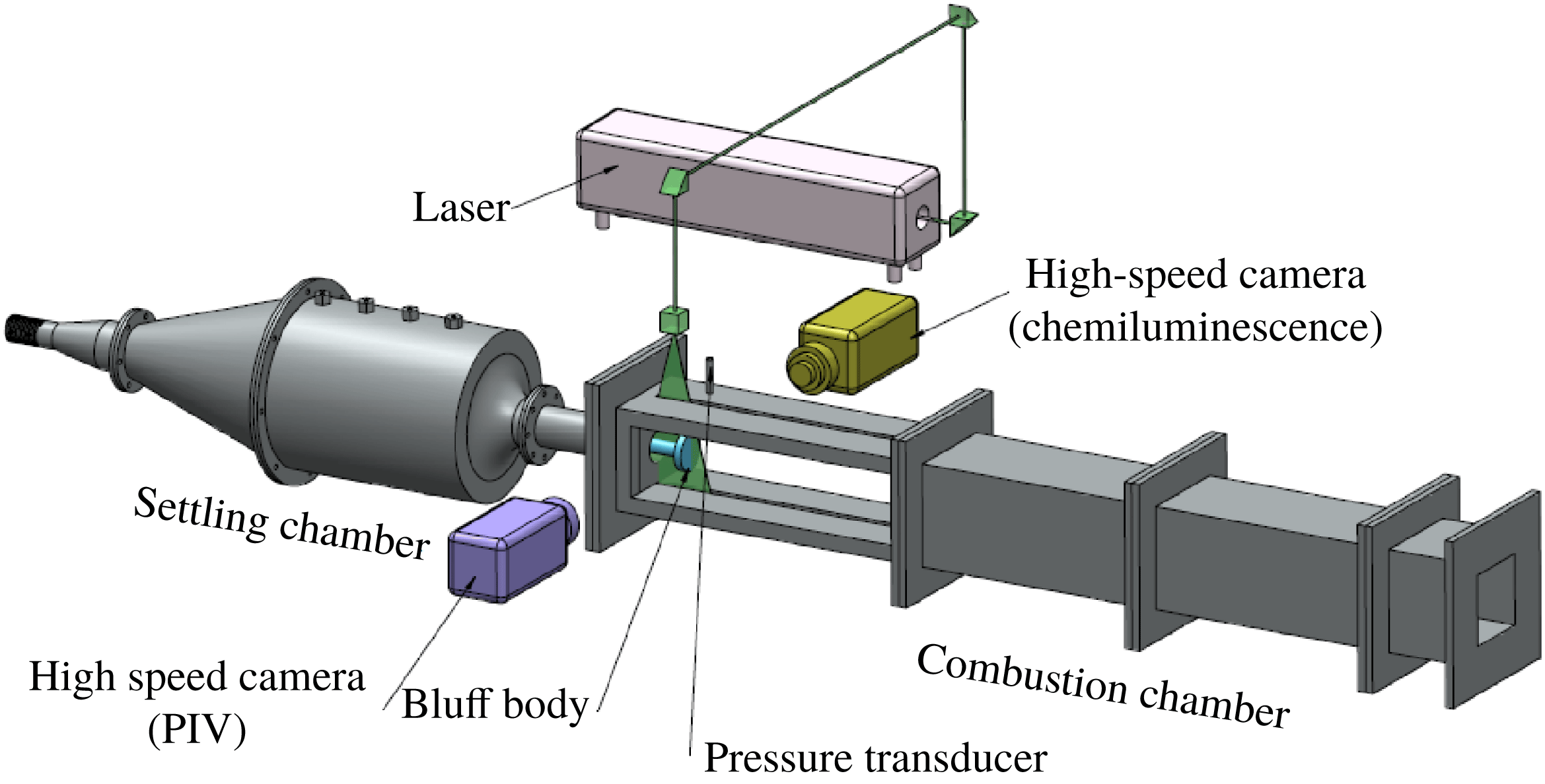
We perform experiments in a backward-facing step combustor with a bluff body as the flame-holding device at high Reynolds number. The experimental set-up, as shown in figure 1, mainly consists of three parts – a settling chamber, a burner and a rectangular combustion chamber. More details regarding the experimental set-up can be found in Nair et al. (Reference Nair, Thampi, Karuppusamy, Gopalan and Sujith2013).
The schematic of the experimental set-up used in the current study. The design of the combustor was adapted from Komarek & Polifke (Reference Komarek and Polifke2010).

The air used for combustion enters the test section through the settling chamber. A blowdown mechanism is used to supply air from high-pressure tanks. A moisture separator removes the water content present in the compressed air before it enters the settling chamber. The settling chamber removes the fluctuations in the inlet air and hence decouples its effect on the spatiotemporal dynamics in the combustion chamber. Liquefied petroleum gas (LPG, 60 % butane and 40 % propane) is used as the fuel in the experiments. The fuel is injected into the burner, at 120 mm upstream of the bluff body, through four radial holes of 1.7 mm diameter using a central shaft. A circular disk of 2 mm thickness and 40 mm diameter with 300 holes of 1.7 mm diameter is located 30 mm downstream of the fuel injection location to act as a flashback arrestor. The combustion chamber consists of a sudden expansion from the circular burner of 40 mm diameter to a square cross-section of 90 mm
 $\times$
90 mm and a length of 1100 mm. The partially premixed fuel–air mixture is spark-ignited in the recirculation zone of the dump plane using an 11 kV ignition transformer. A circular disk (bluff body) of 40 mm diameter and 10 mm thickness is used for flame stabilization. The bluff body is attached at the end of the central shaft and is located at a distance of 45 mm downstream of the backward-facing step.
The control parameter in the experiment is the equivalence ratio (
 $\unicode[STIX]{x1D719}=({\dot{m}}_{fuel}/{\dot{m}}_{air})_{actual}/({\dot{m}}_{fuel}/{\dot{m}}_{air})_{\mathit{stoichiometry}}$
), which is varied by keeping the fuel flow rate constant at 30 SLPM and increasing the air flow rate. The air and fuel flow rates are measured using mass flow controllers (Alicat Scientific, MCR Series, 100 SLPM model for fuel flow, 2000 SLPM for air flow; uncertainty is
 $\pm$
(0.8 % of reading
 $+$
0.2 % of full scale)). Throughout the experiments, the flow is turbulent (
 $Re$
ranges from
 $1.9\times 10^{4}$
to
 $3\times 10^{4}$
, with an uncertainty ranging from
 $\pm 314$
to
 $\pm 400$
). The unsteady pressure is measured using a piezoelectric transducer (PCB 103B02, with a sensitivity of
 $223.4~\text{mV}~\text{kPa}^{-1}$
and an uncertainty of
 $\pm 0.15$
Pa), located at a distance of 40 mm downstream of the dump plane at a sampling frequency of 10 kHz for 3 s. A pair of quartz windows (
 $400~\text{mm}\times 90~\text{mm}\times 10~\text{mm}$
) is provided in the side walls of the combustion chamber to facilitate optical diagnostics. A high-speed CMOS camera (Phantom-v 12.1) is used to capture the
 $\text{OH}^{\ast }$
chemiluminescence from the flame, with a narrow band filter centred at 308 nm (12 nm FWHM). The flame images are recorded at a sampling frequency of 2 kHz, with an exposure time of
 $500~\unicode[STIX]{x03BC}\text{s}$
and a resolution of 800 pixels
 $\times$
600 pixels. The camera is outfitted with a 50 mm ZEISS camera lens at
 $f/2$
aperture. A total of 5034 images is acquired for each equivalence ratio that covers the transition of the turbulent combustor from combustion noise to thermoacoustic instability via intermittency.
We seed the flow with
 $\text{TiO}_{2}$
particles (Kronos, product 1071) of diameter
 $1~\unicode[STIX]{x03BC}\text{m}$
to obtain the Mie scattering images for the high-speed PIV. A single-cavity double-pulsed Nd:YLF laser (Photonics) with a wavelength of 527 nm and a pulse duration of 10 ns is used to illuminate the particle seeded flow. The repetition rate of each of the two pulses is 2 kHz. A second high-speed CMOS camera (Photron FASTCAM SA4), synchronized with the laser, outfitted with a ZEISS camera lens of 100 mm focal length with an aperture at
 $f/5.6$
, is used to acquire the Mie scattering images at a frame rate of 1000 Hz. The measurement domain with a resolution of 640 pixels
 $\times$
480 pixels, located at the centre span of the bluff body, has a physical dimension of length 57 mm and width 33 mm. A bandpass optical filter centred at 527 nm is mounted in front of the camera to filter the flame and other background luminosity. A detailed description of the analysis of PIV with the post-processing algorithms that are used to detect spurious vectors can be found in Unni et al. (Reference Unni, Krishnan, Manikandan, George, Sujith, Marwan and Kurths2018). Simultaneous acoustic pressure measurement,
 $\text{OH}^{\ast }$
chemiluminescence imaging and PIV were performed for different equivalence ratios during the intermittency route to thermoacoustic instability.
3 Network construction
In order to study the spatiotemporal evolution of acoustic power sources, we perform simultaneous high-speed chemiluminescence (
 $\text{OH}^{\ast }$
) imaging of the combustion zone, near the dump plane of the combustor, along with the acoustic pressure measurement at different equivalence ratios during the transition from combustion noise to thermoacoustic instability via intermittency. The
 $\text{OH}^{\ast }$
chemiluminescence serves as a marker for the heat release rate from the flame as the
 $\text{OH}^{\ast }$
intensity depends upon the chemical reaction rate (Hurle et al.
Reference Hurle, Price, Sugden and Thomas1968; Nori & Seitzman Reference Nori and Seitzman2008). Even though the flow field is three-dimensional inside the combustor, we analyse it in a two-dimensional plane focused on the central plane of the combustor, with a depth of focus of 9 mm. The raw images of resolution 800 pixels
 $\times$
600 pixels are cropped to a physical dimension of 57 mm
 $\times$
33 mm, located at a distance of 28 mm downstream of the dump plane. We chose this region for the spatiotemporal analysis as it depicts interesting flow and flame dynamics during the different regimes of combustor operation (Unni & Sujith Reference Unni and Sujith2017).
We measure the unsteady pressure
 $p^{\prime }(t)$
at a point near the dump plane. Nair et al. (Reference Nair, Thampi and Sujith2014) reported that the pressure variation across the combustion zone, in the present experimental set-up, is very small. Hence, we assume the pressure to be constant in the measurement domain at a given instant of time. In order to characterize the spatiotemporal evolution of acoustic power sources during a dynamical state of combustor operation, we multiply the unsteady heat release rate field
 $\dot{q}^{\prime }(x,y,t)$
, obtained from the
 $\text{OH}^{\ast }$
chemiluminescence images, with the unsteady pressure at the corresponding time instant. In this manner, we obtain a series of 5026
 $p^{\prime }\dot{q}^{\prime }$
images for a particular state of combustor operation. This is repeated for different equivalence ratios as the combustor transits from combustion noise to thermoacoustic instability via intermittency.
The product of
 $p^{\prime }$
and
 $\dot{q}^{\prime }$
represents the local acoustic power (Putnam Reference Putnam1971; Poinsot & Veynante Reference Poinsot and Veynante2005). Each pixel of the
 $p^{\prime }\dot{q}^{\prime }$
image represents a local acoustic power source if the value of
 $p^{\prime }\dot{q}^{\prime }$
is positive or a local acoustic power sink if it is negative or zero. For the time-varying spatial network analysis, we consider each pixel of the
 $p^{\prime }\dot{q}^{\prime }$
image to be a node. Two nodes are connected if and only if the values of
 $p^{\prime }\dot{q}^{\prime }$
at these two nodes are positive. As we connect only those nodes where
 $p^{\prime }\dot{q}^{\prime }$
are positive, we track the spatiotemporal evolution of only the acoustic power sources. Since the turbulent combustor is a fluid mechanical system where energy transfer takes place locally amongst the fluid elements mainly due to convection, we consider only the nearest neighbours
 $n_{i}$
of a node (the distance between the nodes should not exceed
 $\surd 2$
) when establishing a link. This implies that a node can have a maximum of only eight links. The average value of
 $p^{\prime }\dot{q}^{\prime }$
at the two connecting nodes (i.e. where
 $p^{\prime }\dot{q}^{\prime }$
is positive and the distance between the nodes is less than or equal to
 $\surd 2$
) is considered as the weight of the link between them. At a given value of the control parameter, we obtain high-speed chemiluminescence images for a duration of 2.513 s (with a sampling frequency of 2000 frames per second). Hence, at a given value of the control parameter, we have 5026 high-speed flame images and therefore 5026 time-varying weighted spatial acoustic power networks. In this manner, we construct 5026 time-varying weighted spatial networks for each equivalence ratio.
In order to characterize the spatiotemporal evolution of acoustic power sources, we use one of the basic weighted network measures – the node strength (Boccaletti et al.
Reference Boccaletti, Latora, Moreno, Chavez and Hwang2006). The node strength (
 $s$
) of a given node
 $i$
is defined as the sum of the weights of the links of a node. It is given by
 $$\begin{eqnarray}s_{i}=\mathop{\sum }_{j\in n_{i}}w_{ij},\end{eqnarray}$$
where
 $i$
and
 $j$
represent nodes of the network,
 $w$
the weight of the link connecting
 $i$
and
 $j$
and
 $n_{i}$
the neighbourhood of the node
 $i$
. A node having higher node strength implies that the links of the given node carry higher weights. Since, in the present study, the weight of the link refers to the average value of
 $p^{\prime }\dot{q}^{\prime }$
at the two connecting nodes, regions of high node strength represent regions of high local acoustic power production.
Unni & Sujith (Reference Unni and Sujith2017) observed that vortices play a significant role in determining the flame dynamics during combustion noise, intermittency and thermoacoustic instability, as mentioned in § 1. Hence, it is imperative that we analyse the vorticity field along with the heat release rate field to understand better the spatiotemporal evolution of the local acoustic power sources. Thus, we construct time-varying weighted spatial networks from the vorticity field, obtained from the analysis of PIV, along with the time-varying local acoustic power networks. The region of interest (ROI) considered for the analysis of PIV is the same as the one used for high-speed chemiluminescence imaging. In the analysis of PIV, the ROI in the flow field is divided into a rectangular grid. Each of the cells of this rectangular grid is known as an interrogation window (Raffel, Willert & Kompenhans Reference Raffel, Willert and Kompenhans2007). From the analysis of PIV, we obtain a velocity vector in each of these interrogation windows at every time instant. We consider these interrogation windows as the nodes of the vorticity network. Two nodes are connected if and only if the vorticity values (
 $\unicode[STIX]{x1D714}$
) at these nodes are either both positive or both negative. This implies that two nodes
 $i$
and
 $j$
are connected if
 $\unicode[STIX]{x1D714}_{i}$
,
 $\unicode[STIX]{x1D714}_{j}>0$
or
 $\unicode[STIX]{x1D714}_{i},\unicode[STIX]{x1D714}_{j}<0$
. Similar to the acoustic power network, here also, we only consider the nearest neighbours
 $n_{i}$
of a node when establishing a link (the distance between the two nodes should not exceed
 $\text{ }\surd 2$
). Hence, a node can have a maximum of only eight connections. The average vorticity (
 $(\unicode[STIX]{x1D714}_{i}+\unicode[STIX]{x1D714}_{j})/2$
) at the two connecting nodes is considered as the weight of the link between them. Positive values of node strength denote regions of anticlockwise vorticity (
 $\unicode[STIX]{x1D714}>0$
) and negative values of node strength denote regions of clockwise vorticity (
 $\unicode[STIX]{x1D714}<0$
). In this manner, we construct both the acoustic power and the vorticity network at every instant of time for each of the equivalence ratios as the turbulent combustor transits from combustion noise to thermoacoustic instability via intermittency.
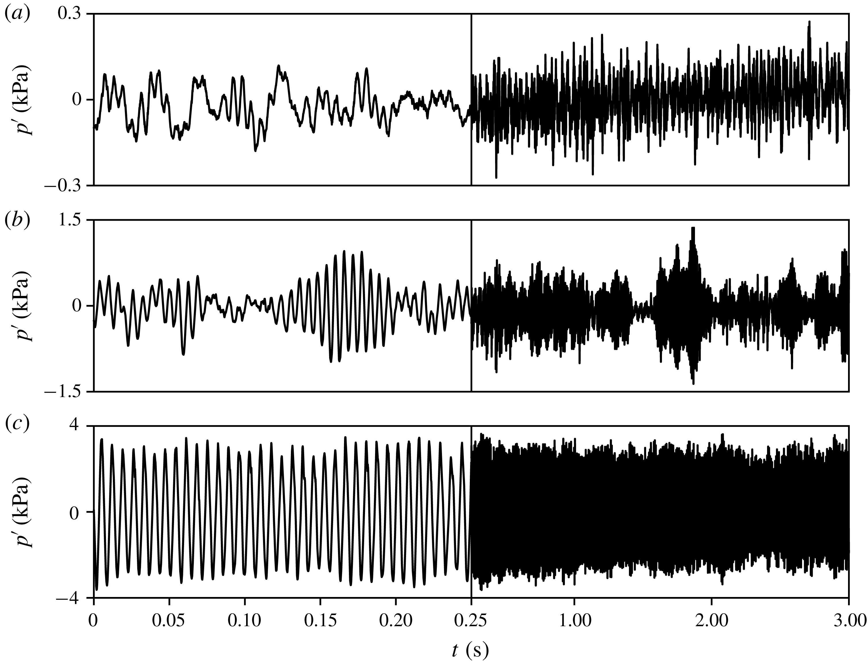
The time series of acoustic pressure obtained from the experiments during (a) combustion noise (
 $\unicode[STIX]{x1D719}=0.97$
), (b) intermittency (
 $\unicode[STIX]{x1D719}=0.81$
) and (c) thermoacoustic instability (
 $\unicode[STIX]{x1D719}=0.62$
). During combustion noise, the pressure fluctuations have low amplitude and are aperiodic in nature. During intermittency, we observe high-amplitude bursts of periodic oscillations embedded amidst epochs of low-amplitude aperiodic fluctuations. Thermoacoustic instability is characterized by high-amplitude periodic oscillations with a frequency of 142 Hz. The equivalence ratio is reduced by keeping the fuel flow rate constant and increasing the air flow rate.

4 Results and discussion
The thermoacoustic system in a turbulent combustor transits from combustion noise to thermoacoustic instability via a dynamical state called intermittency (Nair et al.
Reference Nair, Thampi and Sujith2014). The time trace of pressure fluctuations during the different dynamical states of combustor operation is shown in figure 2, wherein the equivalence ratio is varied from near stoichiometry to lean blowoff conditions. When the equivalence ratio is near stoichiometry (
 $\unicode[STIX]{x1D719}=0.97$
), the temporal dynamics of the combustor is characterized by low-amplitude aperiodic pressure fluctuations. This stable state of combustor operation is called combustion noise (Strahle Reference Strahle1971). As the equivalence ratio is reduced, the turbulent combustor exhibits intermittency. During intermittency (
 $\unicode[STIX]{x1D719}=0.81$
), the time series of acoustic pressure consists of bursts of high-amplitude periodic oscillations sandwiched between epochs of low-amplitude aperiodic fluctuations in a seemingly random manner. On further reduction of the equivalence ratio (
 $\unicode[STIX]{x1D719}=0.62$
), the onset of thermoacoustic instability occurs, which is characterized by high-amplitude periodic pressure oscillations. In the current study, we construct time-varying weighted local acoustic power and vorticity networks during combustion noise, intermittency and thermoacoustic instability. Using the measures from complex network theory, we first examine the spatiotemporal evolution of acoustic power sources visually and then obtain some statistical measures to quantify the dynamics.
4.1 Spatiotemporal evolution of acoustic power sources during combustion noise and thermoacoustic instability
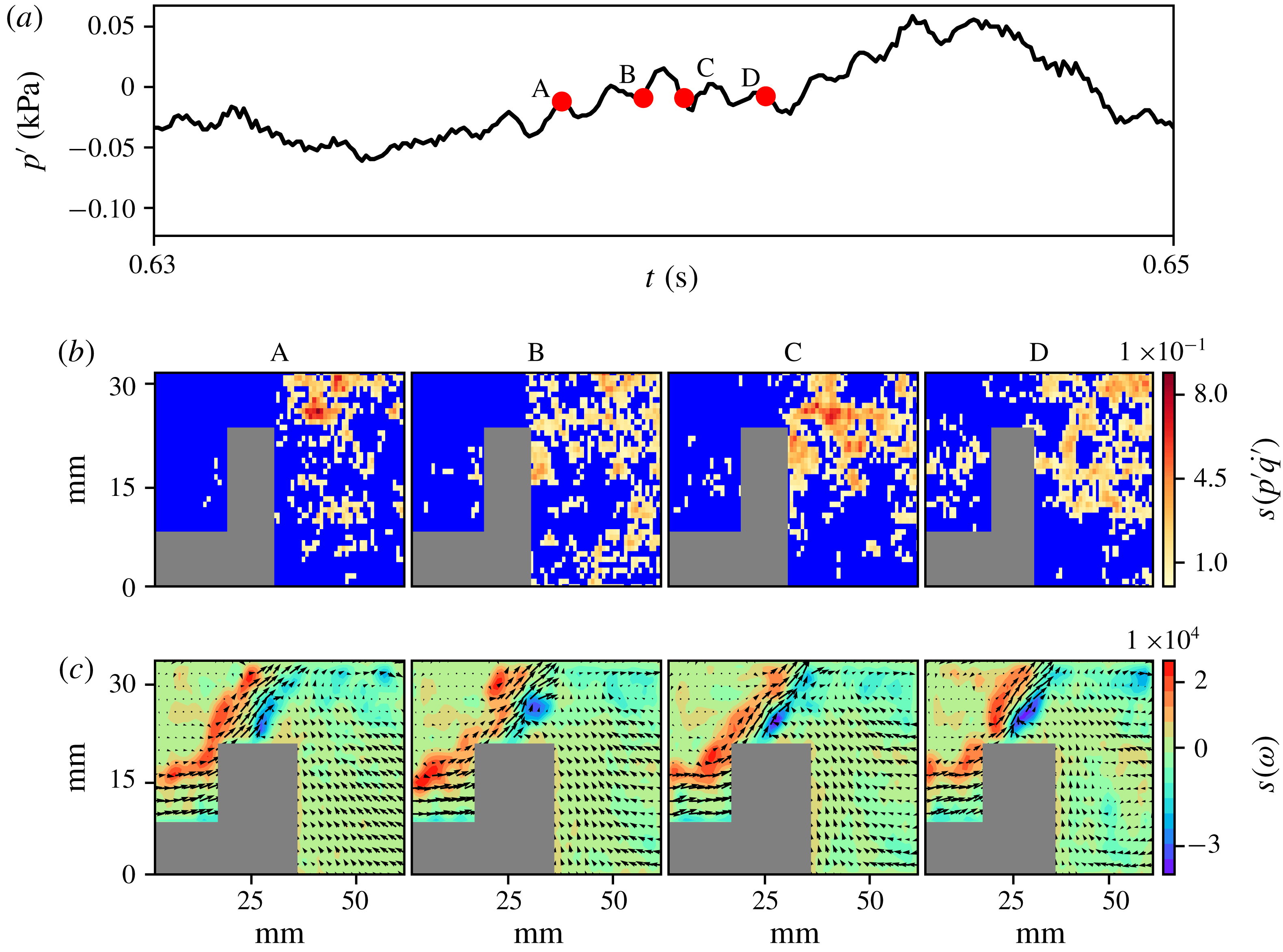
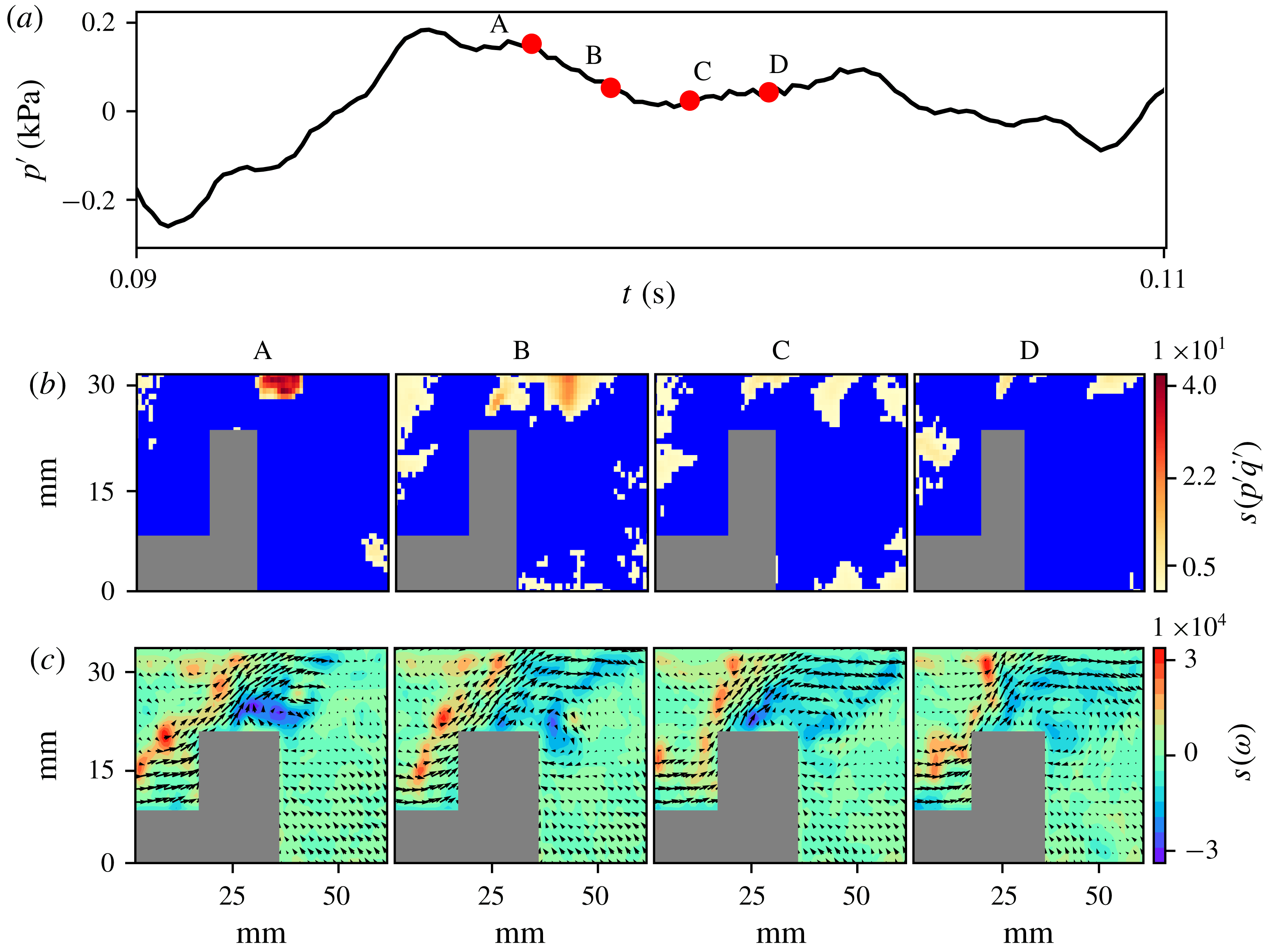
We first examine the spatiotemporal evolution of the acoustic power sources during combustion noise (stable combustion) and thermoacoustic instability (unstable combustion). The spatial distributions of the node strengths (3.1) of the acoustic power and the vorticity networks at different time instants during combustion noise are shown in figure 3. In the acoustic power network (figure 3
b), the blue colour represents the local acoustic power sinks. The colourbar indicates the magnitude of node strength, which corresponds to the local acoustic power production in the turbulent reactive flow field. The spatial distribution of the node strength reveals that the acoustic power production happens in small fragmented clusters during combustion noise. The distribution of the local acoustic power sources resembles small islands scattered in an ocean of acoustic power sinks. In the vorticity network (figure 3
c), the node strength gives the average vorticity in the immediate neighbourhood of a node. Velocity vectors obtained from the analysis of PIV are superimposed onto the vorticity network to understand the flow field better. High values of positive node strength (denoted by red regions) indicate the presence of a train of small discrete vortices in the outer shear layer. High values of negative node strength (denoted by blue regions) in the inner shear layer represents the small vortices shed from the tip of the bluff body. The grey colour mask in the subplots (figures 3
b and c) represents the bluff body. The bluff body shape in figures 3(b) and (c) looks dissimilar due to the fact that in figure 3(b) the nodes are the pixels whereas in figure 3(c), the nodes are the interrogation windows used in the analysis of PIV. The size of the interrogation windows is 32 pixels
 $\times$
32 pixels (Unni et al.
Reference Unni, Krishnan, Manikandan, George, Sujith, Marwan and Kurths2018). Hence, the area that a node occupies in figure 3(c) is bigger than that in figure 3(b). Also, in figure 3(c), the mask includes the region where laser reflection is high.
The spatial distribution of the node strengths of (b) the acoustic power network and (c) the vorticity network at the corresponding time instants (A, B, C and D) marked on (a) the time series of fluctuating pressure during combustion noise. The blue region in the spatial distribution of the node strength of the acoustic power (
 $p^{\prime }\dot{q}^{\prime }$
) network represents local acoustic power sinks. The colourbar in (b) represents the magnitude of the node strength, which indicates the average acoustic power produced in the neighbourhood of a node. The spatial distribution of the node strength shows that acoustic power production happens in small disconnected fragments during combustion noise. In the vorticity network (c), the node strength indicates the average vorticity in the neighbourhood of a node. Positive values of node strength represent the vorticity distribution in the anticlockwise direction, whereas negative node strength indicates the vorticity distribution in the clockwise direction. Velocity vectors are superimposed onto the vorticity network to understand the flow field better. Small vortices are present in the outer shear layer as well, as they are being shed from the tip of the bluff body. The grey rectangles in the subplots represent the bluff body.

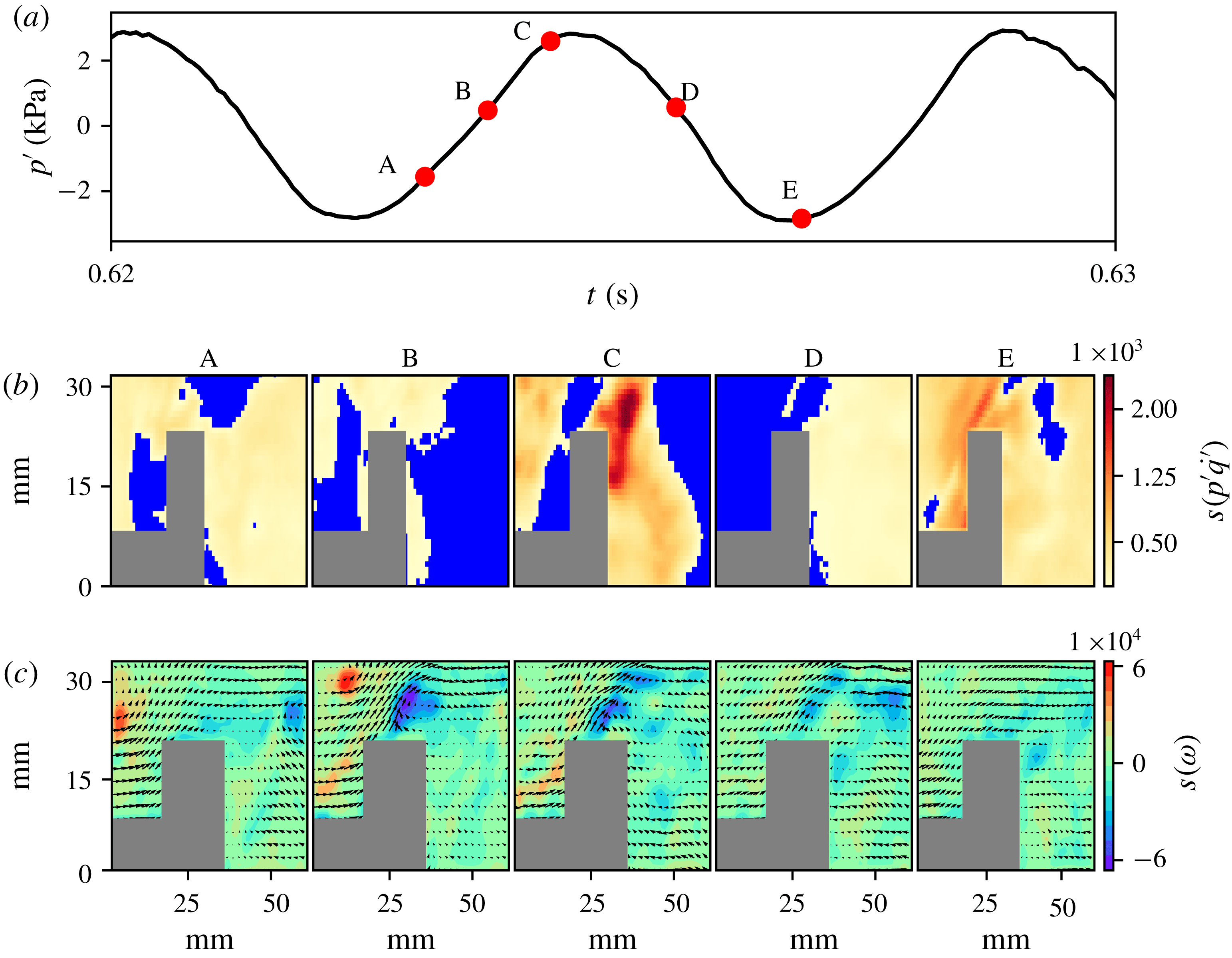
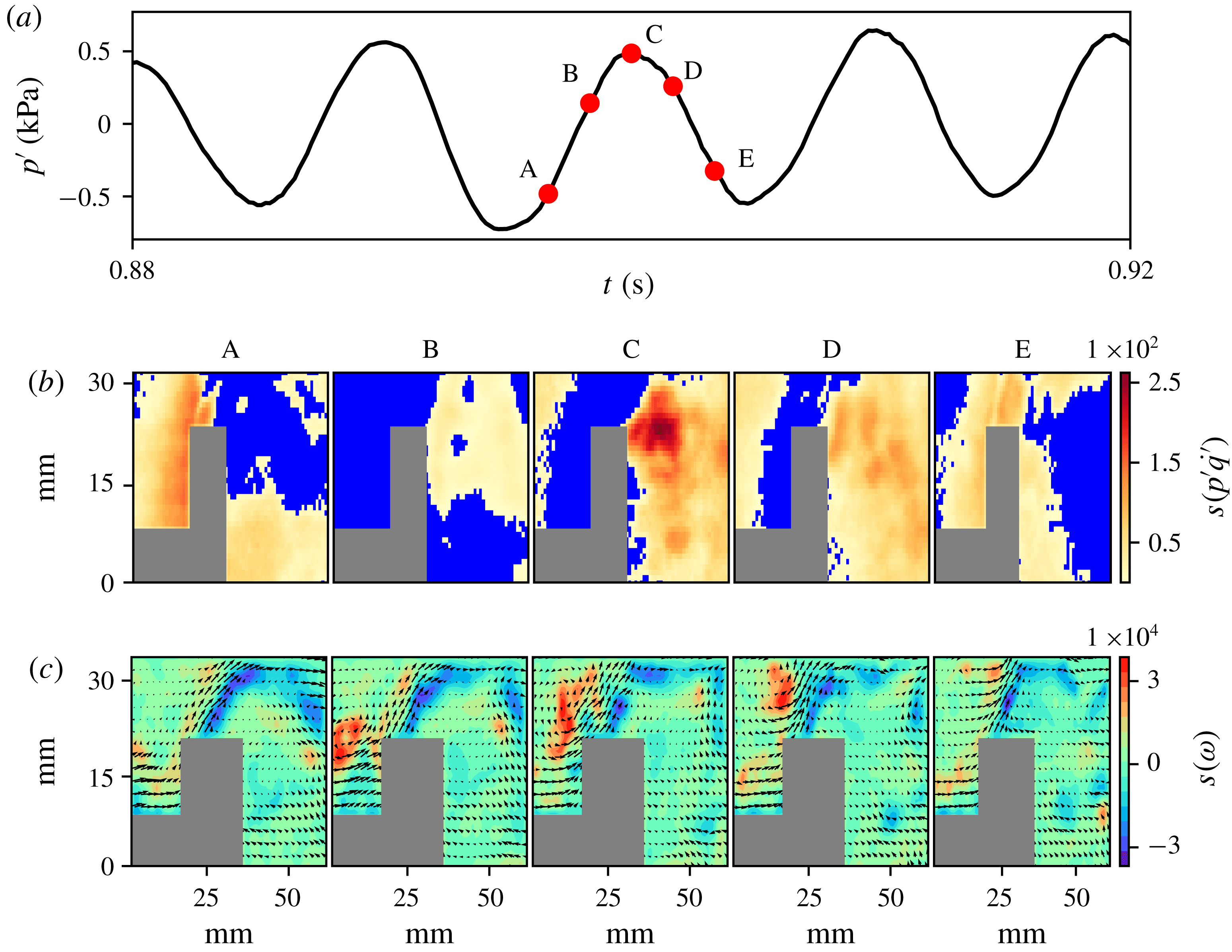
The spatial distribution of the node strengths of (b) the acoustic power network and (c) the vorticity network at the corresponding time instants (A, B, C, D and E) marked on (a) the time series of oscillating pressure during thermoacoustic instability. The spatial distribution of the node strength of the acoustic power network indicates that during thermoacoustic instability, the acoustic power production occurs in large clusters. The high values of positive node strength of the vorticity network coincide with the centre of the coherent structure formed downstream of the dump plane. The maximum acoustic power production occurs when the coherent structure impinges on the top wall of the combustor (C). The magnitude of acoustic power production during thermoacoustic instability is almost three orders of magnitude higher than that during combustion noise, as indicated by the node strength of the acoustic power network.

In figure 4, the spatial distributions of the node strengths of the acoustic power and the vorticity networks at different time instants during a periodic cycle of thermoacoustic instability are shown. Unlike the situation during combustion noise, the acoustic power production happens now in large clusters during thermoacoustic instability (figure 4 b). The acoustic power production during thermoacoustic instability is around three orders of magnitude higher than that during combustion noise, as indicated by high values of node strength. High values of positive node strength in the vorticity network (at time instants A and B in figure 4 c) coincide with the centre of the coherent structure being formed downstream of the bluff body. The coherent structure begins to form at the dump plane, when the acoustic pressure fluctuation is near local minima (E). As the coherent structure convects downstream it grows in size. The formation of large coherent structures at the onset of thermoacoustic instability has been reported in earlier studies, as discussed in § 1. The maximum acoustic power production occurs when the large coherent structure impinges on the top combustor wall.
As the coherent structure convects towards the top of the bluff body (from time instants A to C in figure 4 c), the region between the outer and inner shear layer is compressed against the rear end of the bluff body. This increases the shear strain, which leads to local extinction (Hult et al. Reference Hult, Meier, Meier, Harvey and Kaminski2005). This may be the reason for almost no reaction to take place just upstream of the bluff body, leading to the presence of local acoustic power sinks in the rear end of the bluff body, above the bluff body shaft. As the coherent structure passes over the top of the bluff body, separation of the inner shear layer from the tip of the bluff body happens. This suggests the frequency of formation of the coherent structure downstream of the dump plane and the large vortex from the tip of the bluff body to be almost identical. High values of negative node strength in the vorticity network indicate the shedding of these large vortices from the tip of the bluff body. As the large vortex convects downstream of the bluff body, the region between the outer and the inner shear layer expands. This is accompanied by a flow reversal at the bluff body due to volume expansion because of intense heat release, as well as the reversal of acoustic velocity. This inhibits the flow of fresh reactant mixture into the combustion zone. This is the reason why we have large clusters of acoustic power sources in the flow field when the acoustic pressure fluctuation is negative (see time instants E and A in figure 4 b). When the pressure inside the combustion chamber becomes very low, the flow surges back into the combustion chamber. As the acoustic mode is reinforced by the intense in-phase heat release rate, the velocity fluctuation amplitude increases. This induces the formation of a large coherent structure downstream of the dump plane and the cycle continues.
4.2 Spatiotemporal evolution of acoustic power sources during intermittency
Next, we examine the spatiotemporal evolution of the acoustic power sources during intermittency. Intermittency can be viewed, in simple terms, as a tug of war between the acoustic driving and the acoustic damping present in the system. As the acoustic driving wins over the damping, the growth of the acoustic pressure oscillations occurs. As the damping overtakes the driving, these high-amplitude acoustic pressure oscillations start to decay. It is this competition between the acoustic driving and the damping that leads to the emergence of bursts of high-amplitude periodic oscillations in the background of low-amplitude aperiodic pressure oscillations during intermittency.
In this section, we will see how spatially continuous large clusters of acoustic power sources emerge at the onset of thermoacoustic instability from the small fragmented clusters of acoustic power sources observed during combustion noise. To that end, we investigate the spatial and temporal evolution of acoustic power sources during an aperiodic epoch of intermittency and a periodic epoch of intermittency, the growth of low-amplitude aperiodic pressure fluctuations to high-amplitude periodic oscillations and the decay of high-amplitude periodic pressure oscillations to low-amplitude aperiodic fluctuations. In figure 5, we show the spatiotemporal evolution of acoustic power sources during an aperiodic epoch of intermittency. In this case, similar to the one observed during combustion noise, the acoustic power production happens in small fragmented clusters or islands scattered in an ocean of acoustic power sinks.
Next, we examine the spatiotemporal evolution of acoustic power sources during a periodic epoch of intermittency, as shown in figure 6. We observe coherent structures downstream of the dump plane, as seen during thermoacoustic instability. However, there are a few points to be noted here. Firstly, the size and strength of the coherent structure are not as high as in that observed during thermoacoustic instability. George et al. (Reference George, Unni, Raghunathan and Sujith2018) quantitatively measured the size of the coherent structures during the different stages of combustor operation using a vortex detection technique. Also, the strength of the coherent structure, which is reflected in the magnitude of the positive node strength, is lower than that during thermoacoustic instability. More significantly, the coherent structure impinges on the rear-end tip of the bluff body (see time instant C in figure 6 c) and not on the top wall of the combustor. After impingement, the coherent structure breaks down into small vortices. Since the area of impingement of the coherent structure is lower, the heat release rate that follows is not as intense as in the case of thermoacoustic instability. It is to be noted that these coherent structures are not consistently observed during the periodic epochs of intermittency. They are mostly observed during the high-amplitude peaks of the periodic epochs of intermittency. Here also, we observe the shedding of large vortices from the tip of the bluff body. It is to be noted that the size of the clusters of the acoustic power sources is not as large as that observed during thermoacoustic instability.
The spatial distribution of the node strengths of (b) the acoustic power network and (c) the vorticity network at the corresponding time instants (A, B, C and D) marked on (a) the time series of fluctuating pressure during the aperiodic regime of intermittency. The acoustic power production happens in small fragmented clusters, as in the case of combustion noise.

The spatial distribution of the node strengths of (b) the acoustic power network and (c) the vorticity network at the corresponding time instants (A, B, C, D and E) marked on (a) the time series of fluctuating pressure during the periodic regime of intermittency. The acoustic power production occurs in large clusters as in the case of thermoacoustic instability. However, unlike the case during thermoacoustic instability, the coherent structure impinges the rear-end tip of the bluff body. After impingement, the coherent structure disintegrates into small vortices that convect over the top of the bluff body.

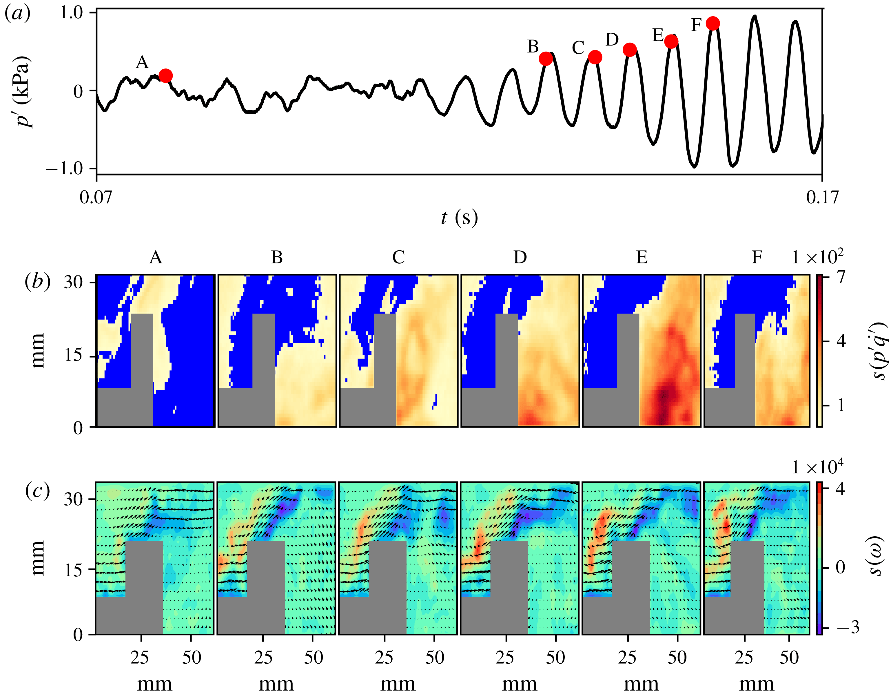
In order to understand how large clusters of acoustic power sources emerge in the flow field during the periodic epoch of intermittency, we examine the spatiotemporal evolution of the acoustic power sources during the growth of low-amplitude aperiodic fluctuations to high-amplitude periodic oscillations, as shown in figure 7. As the pressure oscillations grow, we find the emergence of acoustic power sources at a greater number of spatial locations in the turbulent reactive flow field. We refer to this phenomenon as the nucleation of acoustic power sources in the flow field. Also, as the acoustic pressure amplitude grows, the small fragmented clusters of acoustic power sources coalesce to form large clusters, as reflected in the spatial distribution of the node strength of the acoustic power network (figure 7 b). The mechanism behind the formation of these large clusters can be deduced by examining the vorticity network (figure 7 c). As the acoustic pressure grows, the magnitude of the positive as well as the negative node strength increases; this denotes the increase in the strength of the vorticity field upstream and downstream of the bluff body, respectively.
The spatial distribution of the node strengths of (b) the acoustic power network and (c) the vorticity network at the corresponding time instants (A, B, C, D, E and F) marked on (a) the time series of fluctuating pressure during the growth of pressure oscillations observed during intermittency. As the thermoacoustic system transits from low-amplitude aperiodic oscillations to high-amplitude periodic oscillations during intermittency, the acoustic power sources nucleate, coalesce and grow in size and the strength of acoustic power production also increases.

During the aperiodic epoch of intermittency, a train of small discrete vortices is observed in the outer shear layer downstream of the dump plane. At the same time, small vortices are shed downstream of the bluff body as the inner shear layer gets separated from the tip of the bluff body. As the perturbations near the dump plane increase, these small vortices in the outer shear layer merge to form large vortices. Merging of vortices leads to an increase in fine scale mixing that accelerates combustion (Schadow & Gutmark Reference Schadow and Gutmark1992), thus causing the nucleation of acoustic power sources in the flow field. In addition, as the small vortices merge, coalescence of small fragmented clusters of acoustic power sources occurs. These large vortices convect downstream of the dump plane and impinge on the rear-end tip of the bluff body. Upon impingement, a spike occurs in the heat release rate due to the sudden increased fine scale mixing of the reactants and hot products. This spike in the heat release rate adds energy to the acoustic field, thus acting as a kicked oscillator (Seshadri, Nair & Sujith Reference Seshadri, Nair and Sujith2016). Since the heat release rate occurs in phase with the acoustic pressure oscillation, the amplitude of the acoustic pressure increases, satisfying Rayleigh criteria. This reinforcement of the acoustic mode leads to an increase in the amplitude of velocity fluctuations at the dump plane, thus inducing the formation of a new vortex, and the aforementioned cycle continues. When the perturbation in the flow field is high enough, a large coherent structure forms downstream of the dump plane, gets convected and impinges on the top wall of the combustor. As the large coherent structure carries with it a large pocket of unburnt reactants, upon impingement, the heat release rate is higher. Hence, the energy added to the acoustic field overcomes the damping present in the combustor and the onset of thermoacoustic instability occurs. We note that the convection of the large vortex towards the rear-end tip of the bluff body/top wall of the combustor perturbs the inner shear layer more and hence the size of the vortices shed downstream of the bluff body also increases.
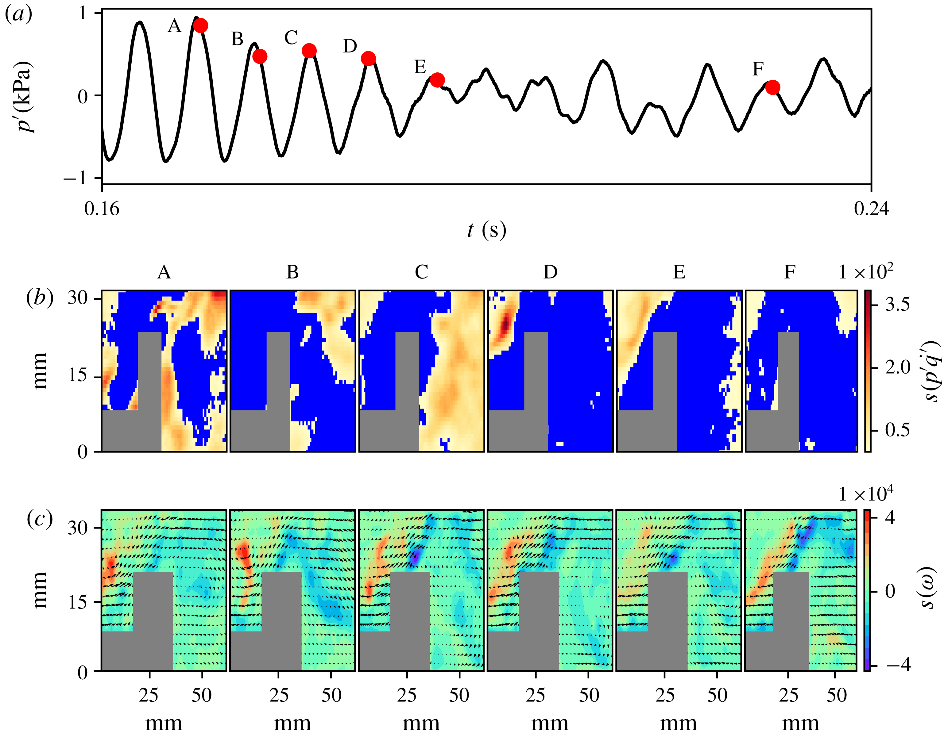
Finally, we examine the spatiotemporal evolution of acoustic power sources during the decay of high-amplitude periodic pressure oscillations to low-amplitude aperiodic pressure fluctuations, as shown in figure 8. During the high-amplitude periodic pressure oscillations, the acoustic power production occurs in large clusters, as evident at time instant A. As the acoustic damping overcomes the acoustic driving in the combustor, the amplitude of the pressure oscillation decays. As the thermoacoustic system transits from high-amplitude periodic oscillations to low-amplitude aperiodic fluctuations, the strength of acoustic power production diminishes and the large clusters disintegrate into small fragmented clusters.
The decay of the acoustic pressure amplitude during intermittency begins to occur once the damping in the turbulent combustor starts to outweigh the acoustic driving. As the damping overcomes the driving, the roll-up of the shear layer into a large vortex, observed during the periodic epochs of intermittency, fails to happen, thus ceasing the formation of large clusters of acoustic power sources. Hence, the amount of energy added to the acoustic field reduces. Henceforth, the periodic epochs of intermittency fail to persist and decay, thus preventing the onset of full-blown thermoacoustic instability.
The spatial distribution of the node strengths of (b) the acoustic power network and (c) the vorticity network at the corresponding time instants (A, B, C, D, E and F) marked on (a) the time series of fluctuating pressure during the decay of pressure oscillations observed during intermittency.

Thus, we observe that the emergence of large clusters of spatially coherent acoustic power sources at the onset of thermoacoustic instability happens via the phenomena of nucleation, coalescence and growth of acoustic power sources. The physical mechanisms behind these phenomena are the merging of small-scale vortices and the formation of larger vortices as the perturbations to the shear layer increase. These findings can be generalized to turbulent thermoacoustic systems involving large-scale vortex shedding. The formation of spatially coherent regions of acoustic power sources at the onset of thermoacoustic instability has also been reported in swirl stabilized combustors (Paschereit, Gutmark & Weisenstein Reference Paschereit, Gutmark and Weisenstein1999; Lee & Santavicca Reference Lee and Santavicca2003; Huang & Ratner Reference Huang and Ratner2009; Tachibana et al. Reference Tachibana, Kanai, Yoshida, Suzuki and Sato2015; Okuno et al. Reference Okuno, Small and Gotoda2015; Kheirkhah et al. Reference Kheirkhah, Geraedts, Saini, Venkatesan and Steinberg2016; Pawaret al. Reference Pawar, Mondal, George and Sujith2018). Hence, we can hypothesize that the phenomena of nucleation, coalescence and growth of acoustic power sources would be happening during intermittency. However, the physical mechanisms leading to the phenomena of nucleation, coalescence and growth may be different as the flow field in a swirl stabilized combustor is different from that observed in a bluff body stabilized combustor.
4.3 Statistical analysis of the clusters of acoustic power sources
In this section, we perform a statistical analysis of the clusters of acoustic power sources as the thermoacoustic system transits from a state of combustion noise to thermoacoustic instability via intermittency. The use of complex network theory enables us to quantify the spatiotemporal evolution of the clusters of acoustic power sources. To that end, we calculate the link density (
 $\unicode[STIX]{x1D70C}$
), the size of the giant cluster (
 $S$
) and the number of clusters (
 $N$
) at different equivalence ratios as the combustor transits from combustion noise to thermoacoustic instability.
Link density refers to the fraction of the links or edges present in the network. If
 $n$
represents the total number of nodes and
 $e$
represents the actual number of links in the network, then link density is given by
 $$\begin{eqnarray}\unicode[STIX]{x1D70C}=\frac{2e}{n(n-1)}.\end{eqnarray}$$
The value of
 $\unicode[STIX]{x1D70C}$
lies between 0 and 1. In simple terms,
 $\unicode[STIX]{x1D70C}$
reflects the number of connections among the nodes of the network. A high value of
 $\unicode[STIX]{x1D70C}$
implies that the network is densely connected and a low value implies that the network is sparsely connected. In the present analysis, a high value of
 $\unicode[STIX]{x1D70C}$
implies that acoustic power production happens in a large number of spatial locations in the flow field as we do not consider acoustic power sinks in the network construction, as explained in § 3.
In graph theory, a connected component of an undirected graph refers to a subgraph in which any two nodes are connected to each other by a path, i.e. a sequence of links (Newman Reference Newman2010). In the present study, the connected components refer to islands or clusters of acoustic power sources. We track the number of such clusters (
 $N$
) as well as the size of the giant cluster (
 $S$
); i.e. the largest connected component of a graph, at each instant of time. In this manner, we obtain, for a given equivalence ratio,
 $\unicode[STIX]{x1D70C}$
,
 $N$
and
 $S$
at every instant of time. Thus, for each equivalence ratio, we construct 2000 acoustic power networks, corresponding to a duration of 1.0 s, as described in § 3.
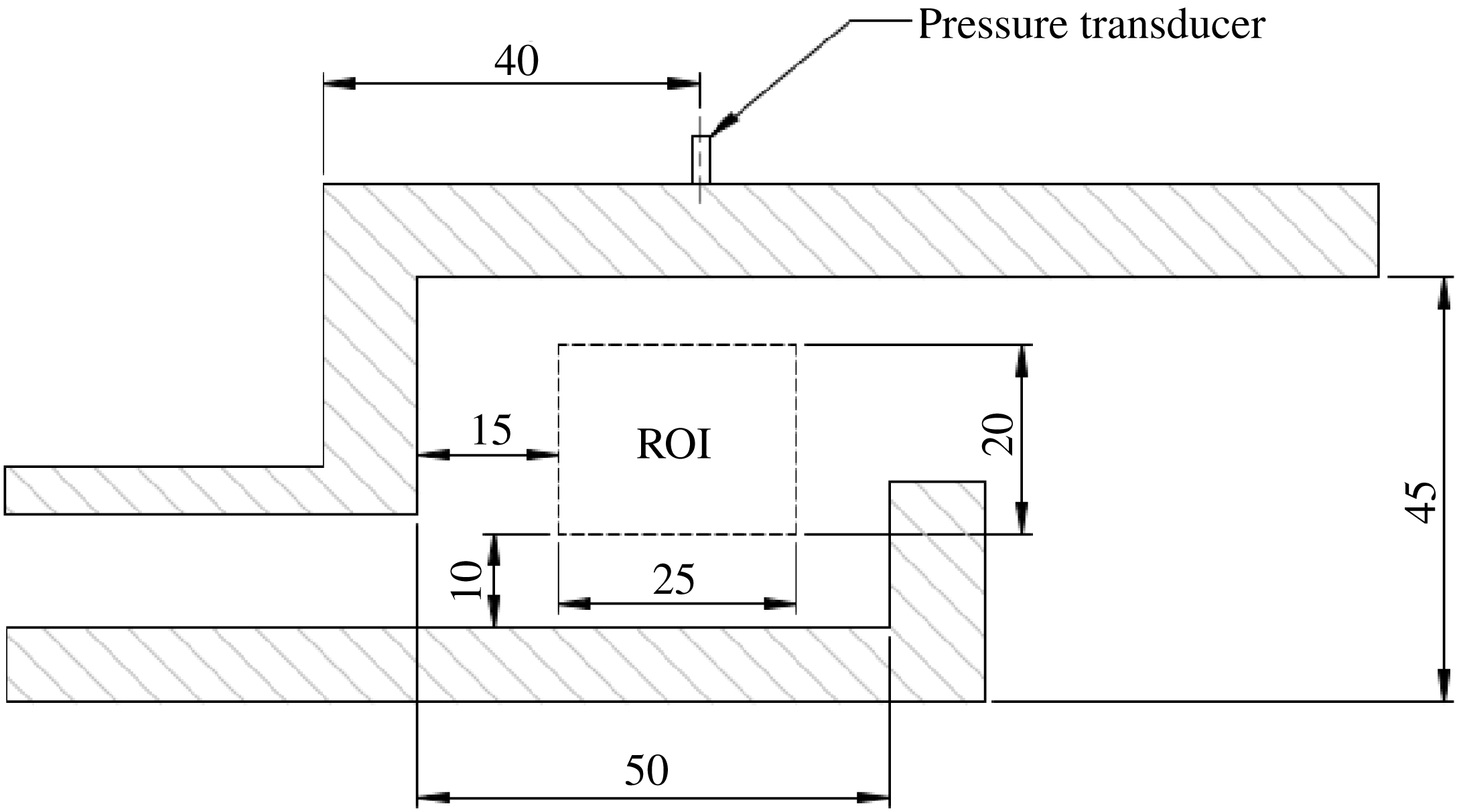
Half cross-section of the combustion chamber showing the ROI, in which the acoustic power network is constructed to compute the network properties. The ROI is chosen such that it coincides with the location of formation of coherent structures downstream of the dump plane. The pressure transducer used for the acoustic pressure measurement is located 40 mm downstream of the dump plane.

Since most of the interesting flow dynamics leading to the coalescence/disintegration of clusters happens upstream of the bluff body, we choose a rectangular ROI upstream of the bluff body for the acoustic power network construction. The chosen ROI, at a distance of 15 mm downstream of the dump plane and 10 mm above the bluff body shaft, has physical dimensions of 25 mm in length and 20 mm in breadth (figure 9). The ROI has a resolution of 225 pixels
 $\times$
180 pixels. Since the calculation of network properties with the original resolution would be computationally very intensive, we downsampled the resolution to 112 pixels
 $\times$
90 pixels (50 % of the original resolution) using bi-cubic interpolation (Zhang et al.
Reference Zhang, Zhao, Zhang, Xiong and Gao2011). Hence, the number of nodes in the network reduces from 40 500 to 10 080. Also, a small threshold (
 $\unicode[STIX]{x1D716}$
) was introduced for the connections among the nodes to prevent the electronic noise of the high-speed camera, used for chemiluminescence measurements, from creeping into the calculation, especially during combustion noise. We choose the threshold for network link connectivity as
 $\unicode[STIX]{x1D716}=1.0$
(around 5 % of the maximum acoustic power production during combustion noise). Hence, two neighbouring nodes are connected if the values of
 $p^{\prime }\dot{q}^{\prime }$
at these nodes are greater than 1.0 instead of 0.0 (without any threshold). The sensitivity of the network properties for different thresholds of network link connectivity (
 $\unicode[STIX]{x1D716}$
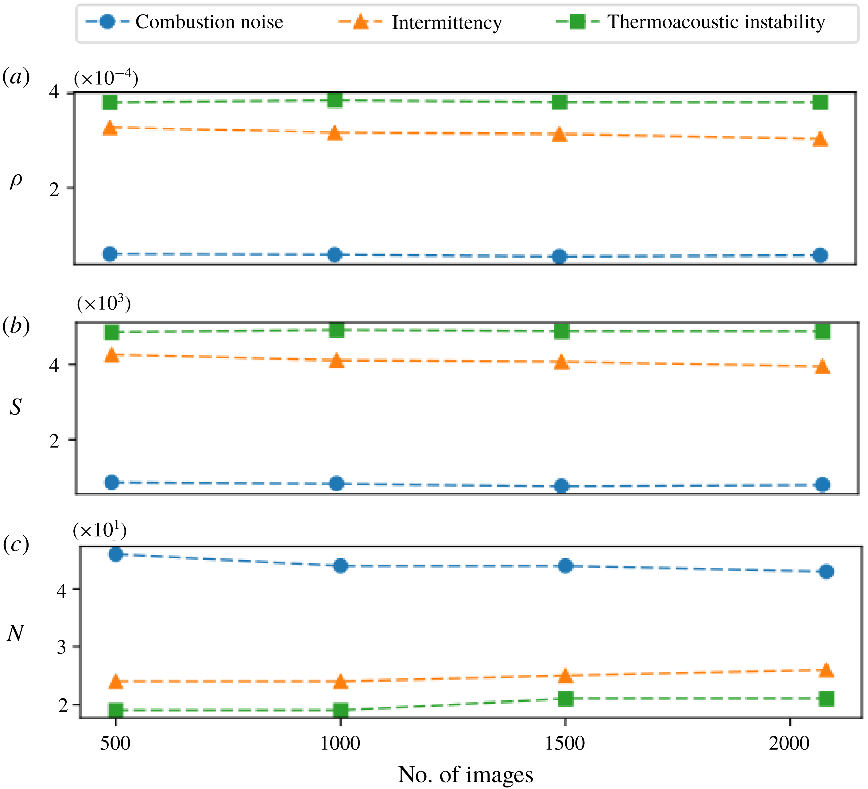
) and the convergence of the network properties with respect to the number of images/networks considered for their calculation are discussed in appendix A (see figures 12 and 13). In this study, we use the NetworkX Python package to calculate the network properties (Hagberg, Swart & Chult Reference Hagberg, Schult, Swart, Varoquaux, Vaught and Millman2008).
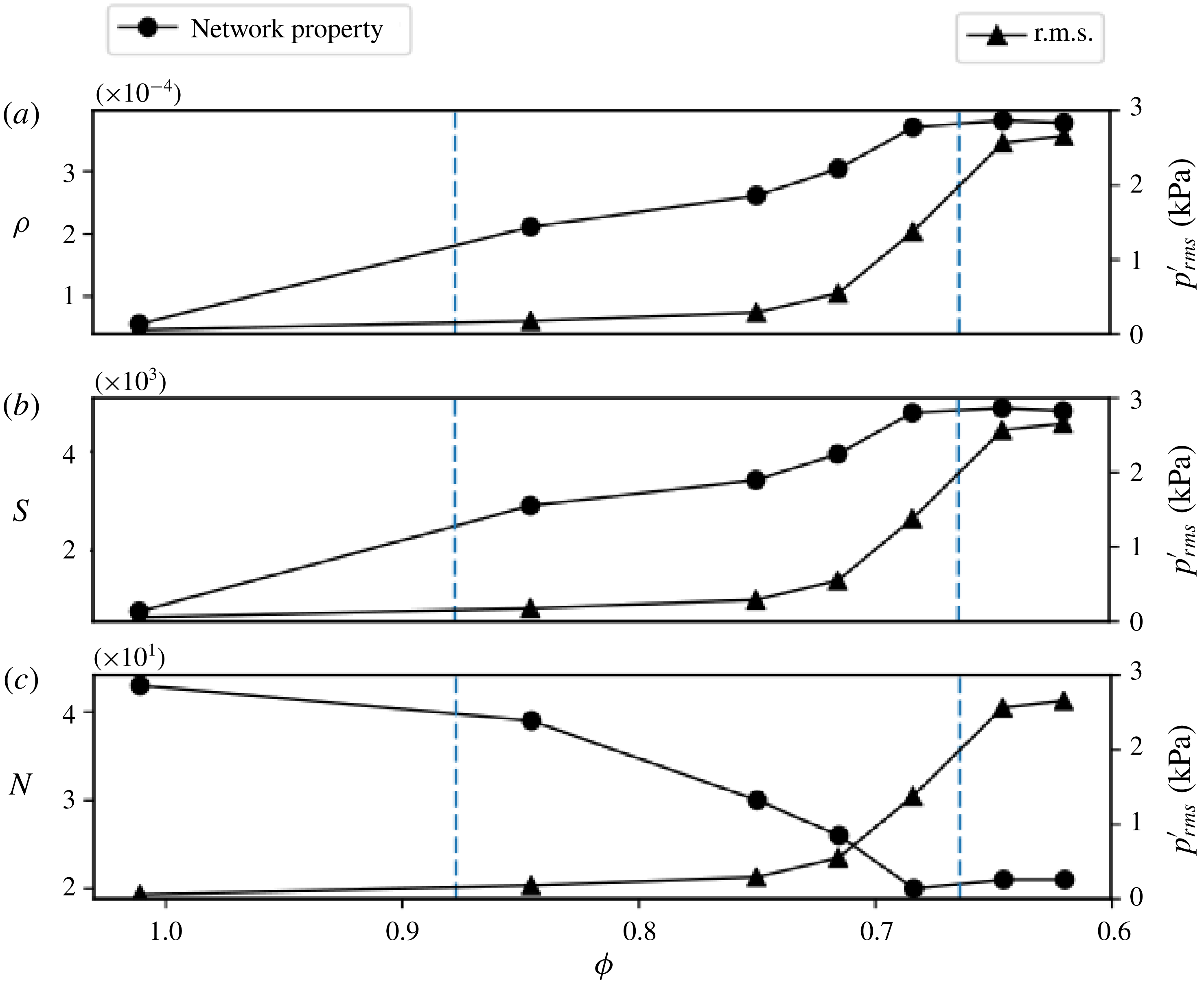
Variation of the temporal mean of the network properties: (a) the link density (
 $\unicode[STIX]{x1D70C}$
), (b) the size of the giant cluster (
 $S$
) and (c) the number of clusters (
 $N$
), along with the variation of the root mean square (r.m.s.) value of the acoustic pressure as the thermoacoustic system transits from combustion noise to thermoacoustic instability via intermittency. The increase in the link density indirectly indicates the increase in the number of locations in the flow field where acoustic power production occurs. The increase in the size of the giant cluster along with the decrease in the number of clusters show that the acoustic power sources coalesce to form large clusters at the onset of thermoacoustic instability. The dashed vertical lines divide the parameter space, i.e. the equivalence ratio
 $(\unicode[STIX]{x1D719})$
, into regimes of combustion noise, intermittency and thermoacoustic instability, respectively.

Figure 10 illustrates the variation of the temporal mean of
 $\unicode[STIX]{x1D70C}$
(figure 10
a),
 $S$
(figure 10
b) and
 $N$
(figure 10
c) of the acoustic power sources at seven different equivalence ratios that cover the transition of the thermoacoustic system from combustion noise to thermoacoustic instability via intermittency. The dashed vertical lines in the plot separate the combustor operational regime into combustion noise, intermittency and thermoacoustic instability, respectively. The variation of the root mean square (r.m.s.) value of the acoustic pressure is also plotted along with the variation of the network properties. As the thermoacoustic system transits from combustion noise to thermoacoustic instability, the average
 $\unicode[STIX]{x1D70C}$
increases sevenfold. This implies that the average number of links during thermoacoustic instability is around seven times that during combustion noise (4.1). A higher value of the average number of links during thermoacoustic instability implies that the acoustic power production occurs at a large number of locations in the flow field when compared to that during combustion noise. This reflects the phenomenon of nucleation of acoustic power sources occurring in the turbulent reactive flow field. The very low value of the average
 $\unicode[STIX]{x1D70C}$
(the maximum value is around 0.0004) is due to the fact that only the nearest neighbours of a node are considered when establishing a link, as mentioned in § 3.
During combustion noise, the acoustic power production happens mostly in a large number of fragmented clusters or islands in an ocean of acoustic power sinks. This explains the presence of a large number of clusters of acoustic power sources during the occurrence of combustion noise in figure 10(c). Mondal et al. (Reference Mondal, Unni and Sujith2017) attributed this spatial incoherence in the acoustic power production to the random distribution of instantaneous phase between the pressure oscillations and the heat release rate oscillations during the occurrence of combustion noise. Also, the average
 $S$
(in figure 10
b) is very small during combustion noise, as the acoustic power production occurs in small fragmented clusters. The average
 $S$
during thermoacoustic instability is approximately six times the value observed during combustion noise. Additionally, we observe only half the average
 $N$
at the onset of thermoacoustic instability when compared to that during combustion noise. These observations clearly show that the large number of fragmented clusters of acoustic power sources observed during combustion noise coalesce to form large clusters at the onset of thermoacoustic instability.
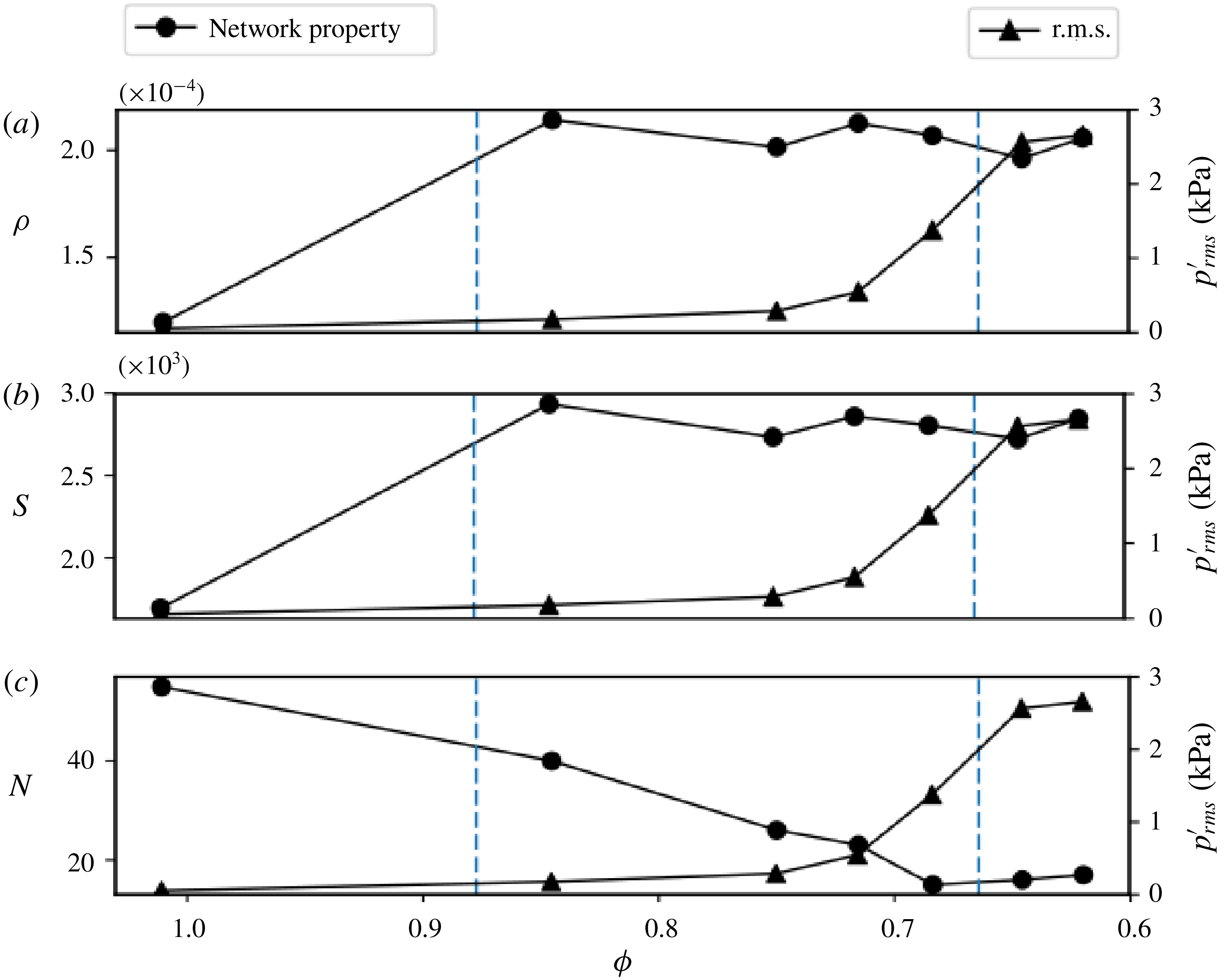
Variation of the standard deviation of the network properties: (a) the link density (
 $\unicode[STIX]{x1D70C}$
), (b) the size of the giant cluster (
 $S$
) and (c) the number of clusters (
 $N$
), along with the variation of the r.m.s. value of the acoustic pressure as the thermoacoustic system transits from combustion noise to thermoacoustic instability via intermittency. The dashed vertical lines divide the parameter space, i.e. the equivalence ratio
 $(\unicode[STIX]{x1D719})$
, into regimes of combustion noise, intermittency and thermoacoustic instability, respectively.

Figure 11 shows the variation of the standard deviation of
 $\unicode[STIX]{x1D70C}$
(figure 11
a),
 $S$
(figure 11
b) and
 $N$
(figure 11
c) of the acoustic power sources, along with the variation of the r.m.s. value of the acoustic pressure. During combustion noise, there are instances where large clusters of acoustic power sources are present in the flow field upstream of the bluff body. However, these large clusters having positive values of
 $p^{\prime }\dot{q}^{\prime }$
occur mostly when the acoustic pressure fluctuation is negative. During combustion noise, most of the reaction occurs in the recirculation zone downstream of the bluff body. In the ROI considered for the calculation of the network properties, which is upstream of the bluff body, not much reaction happens most of the time. Hence, when the acoustic pressure fluctuation (
 $p^{\prime }$
) and the local heat release rate fluctuation (
 $\dot{q}^{\prime }$
) become negative simultaneously, we observe large clusters of acoustic power sources (positive values of
 $p^{\prime }\dot{q}^{\prime }$
) upstream of the bluff body. This explains the high value of the standard deviation for
 $\unicode[STIX]{x1D70C}$
,
 $S$
and
 $N$
during combustion noise. However, we observe high values of standard deviation only for
 $\unicode[STIX]{x1D70C}$
and
 $S$
during intermittency. This can be attributed to the fact that we observe small fragmented clusters of acoustic power sources during the aperiodic epochs of intermittency and large clusters of acoustic power sources during the periodic epochs of intermittency. The standard deviation for the number of clusters of acoustic power sources is low during thermoacoustic instability compared to that during combustion noise (figure 11
c). As discussed earlier, during thermoacoustic instability, the acoustic power production happens mostly in large clusters. Hence, the average number of clusters (see figure 10
c) as well as the standard deviation (figure 11
c) is low during thermoacoustic instability. During one acoustic cycle, when the coherent structure convects out of the ROI towards the top of the bluff body, there will not be many acoustic power sources inside the region of interest. This is the reason for the high value of the standard deviation for link density (figure 11
a) and the size of the giant cluster (figure 11
b) during thermoacoustic instability.
We note that the gradual change in the average network properties happens much before the rise in the r.m.s. of the acoustic pressure as the thermoacoustic system transits from combustion noise to thermoacoustic instability via intermittency (figure 10). This suggests that the transition from small fragmented clusters to large clusters of acoustic power sources is not abrupt. In statistical physics, percolation theory is used in lattice models to study the phenomenon of phase transition. The variation of the size of the giant cluster is used as a marker to study the critical behaviour near the percolation threshold (Newman Reference Newman2010; Barabási Reference Barabási2016). Using complex network theory, researchers have reported percolation-like phase transitions in brain networks (Gallos, Sigman & Makse Reference Gallos, Sigman and Makse2012; Fornito, Zalesky & Bullmore Reference Fornito, Zalesky and Bullmore2016), protein networks (Deb, Vishveshwara & Vishveshwara Reference Deb, Vishveshwara and Vishveshwara2009; Weber & Pande Reference Weber and Pande2015) and recently in climate networks (Lu, Yuan & Fu Reference Lu, Yuan and Fu2016). In the present study, the variation of the average size of the giant cluster (see figure 10 b) reveals a continuous percolation-like phase transition at the onset of thermoacoustic instability in a turbulent combustor. However, a detailed analysis is required to confirm whether this is the case in turbulent combustors with other flame stabilization mechanisms.
5 Conclusions
We used time-varying spatial network analysis of the local acoustic power and the vorticity field in a turbulent combustor with a bluff body stabilized flame during the transition from combustion noise to thermoacoustic instability via intermittency. We find that during combustion noise the acoustic power production occurs in small fragmented clusters, whereas during thermoacoustic instability the acoustic power production happens coherently in large areas. This spatial emergence of large clusters of acoustic power production occurs via nucleation, coalescence and growth of acoustic power sources as the acoustic pressure grows during intermittency. As the acoustic pressure decays, the large clusters of acoustic power sources disintegrate into small fragmented clusters. The presence of large clusters of acoustic power sources during the periodic epochs of intermittency persuades the authors to hypothesize that the disruption of these large clusters can prevent an impending thermoacoustic instability. We quantify the spatiotemporal evolution of the acoustic power sources using network measures such as the link density, the size of the giant cluster and the number of clusters of acoustic power sources. An increase in the link density as well as the size of the giant cluster, along with a decrease in the number of clusters, corroborate our findings. A continuous increase in the size of the giant cluster suggests that the onset of thermoacoustic instability in a turbulent combustor can be viewed as a percolation-like phase transition. The approach presented here can be utilized to study the spatiotemporal evolution of acoustic power sources in combustors with other flame stabilization mechanisms.
Acknowledgements
We acknowledge funding from Siemens Corporate Technology, India, and Office of Naval Research Global (contract monitor Dr R. Kolar). We acknowledge Dr T. Komarek and Professor W. Polifke, TU Munich, Germany, for sharing the design of the combustor. We gratefully thank Dr V. R. Unni and V. Godavarthi for their valuable comments and suggestions that helped in improving the quality of the paper. We also acknowledge Mr N. B. George, Mr R. Manikandan and Mr S. Thilagaraj for help in performing the experiments.
Appendix A
A.1 Sensitivity of network properties with respect to the threshold of network link connectivity (
 $\unicode[STIX]{x1D716}$
)

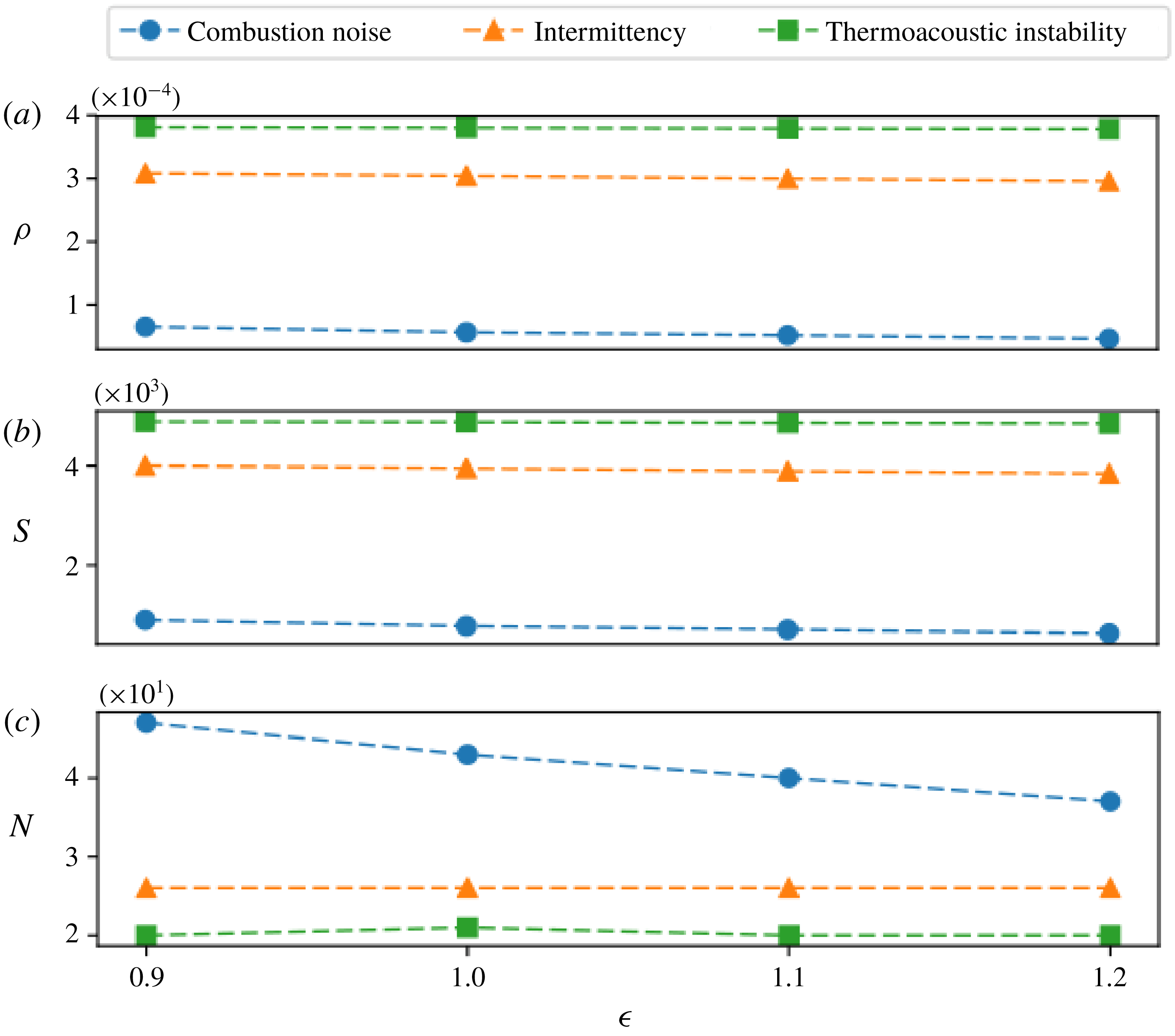
Variation of the temporal mean of the network properties: (a) the link density (
 $\unicode[STIX]{x1D70C}$
), (b) the size of the giant cluster (
 $S$
) and (c) the number of clusters (
 $N$
) with respect to different thresholds of network link connectivity for a case of combustion noise (
 $\unicode[STIX]{x1D719}=1.01$
), intermittency (
 $\unicode[STIX]{x1D719}=0.72$
) and thermoacoustic instability (
 $\unicode[STIX]{x1D719}=0.64$
). Here, the temporal mean is calculated over 2000 images/networks. We observe that the variation in the temporal mean of the network properties for a threshold of 1.0 and above is negligible.

Variation of the temporal mean of the network properties: (a) the link density (
 $\unicode[STIX]{x1D70C}$
), (b) the size of the giant cluster (
 $S$
) and (c) the number of clusters (
 $N$
) calculated over 500, 1000, 1500 and 2080 images/networks for a case of combustion noise (
 $\unicode[STIX]{x1D719}=1.01$
), intermittency
 $(\unicode[STIX]{x1D719}=0.72)$
and thermoacoustic instability (
 $\unicode[STIX]{x1D719}=0.64$
). Here, the threshold for the connectivity of links in the acoustic power network is fixed at 1.0. We observe that the temporal mean of all the network properties for combustion noise, intermittency and thermoacoustic instability remains almost a constant when computed over a total of 1500 images/networks and above.

Figure 12 shows the variation of the temporal mean of the network properties, namely
 $\unicode[STIX]{x1D70C}$
(figure 12
a),
 $S$
(figure 12
b) and
 $N$
(figure 12
c), with respect to different thresholds of network link connectivity (
 $\unicode[STIX]{x1D716}$
) for a case of combustion noise (
 $\unicode[STIX]{x1D719}=1.01$
), intermittency (
 $\unicode[STIX]{x1D719}=0.72$
) and thermoacoustic instability (
 $\unicode[STIX]{x1D719}=0.64$
). The temporal mean is calculated over 2000 images/networks. The average link density and the average size of the giant cluster remain almost a constant for combustion noise, intermittency and thermoacoustic instability for different thresholds of network link connectivity. For the case of combustion noise, we observe a decrease of around 7 % and 7.5 % in the average number of clusters of acoustic power sources when
 $\unicode[STIX]{x1D716}$
is increased from 1.0 to 1.1 and from 1.1 to 1.2, respectively. Nevertheless, the average number of clusters of acoustic power sources does not change for intermittency and thermoacoustic instability for
 $\unicode[STIX]{x1D716}\geqslant 1.0$
. This justifies the use of
 $\unicode[STIX]{x1D716}=1.0$
for the network link connectivity in the current analysis.
A.2 Convergence of network properties with respect to the number of images/networks
Figure 13 shows the variation of the temporal mean of the network properties, namely
 $\unicode[STIX]{x1D70C}$
(figure 13
a),
 $S$
(figure 13
b) and
 $N$
(figure 13
c), calculated over different numbers of images/networks for a case of combustion noise (
 $\unicode[STIX]{x1D719}=1.01$
), intermittency (
 $\unicode[STIX]{x1D719}=0.72$
) and thermoacoustic instability (
 $\unicode[STIX]{x1D719}=0.64$
). The average link density and the size of the giant cluster remain nearly a constant for combustion noise, intermittency and thermoacoustic instability when calculated over the entire range of number of images/networks. The average number of clusters of acoustic power sources saturates for combustion noise, intermittency and thermoacoustic instability when computed over 1500 images/networks and above. This justifies the choice of 2000 images/networks for the computation of the statistical measures of the network properties.