1 Introduction
The dynamics of empty and gas-filled bubbles has been an area of great interest, with applications in fluid dynamics (Brennen Reference Brennen2013), bio-medical physics (Klotz et al. Reference Klotz, Lindvere, Stefanovic and Hynynen2010), condensed matter physics (Browne et al. Reference Browne, Tabor, Chan, Dagastine, Ashokkumar and Grieser2011) and optics (Khalid et al. Reference Khalid, Kappus, Weninger and Putterman2012). The study of the dynamics of a gas-filled cavity immersed in an incompressible liquid was started first by Rayleigh (Reference Rayleigh1917), who derived a collapse time. Liquid viscosity, surface tension and thermal effects were neglected in that early study, and later Plesset & Prosperetti (Reference Plesset and Prosperetti1977) generalized the model to include such terms. The resulting model is a special case of the full Navier–Stokes equations which model the oscillations of a gas-filled spherical cavity immersed in an infinite incompressible fluid, and is therefore nonlinear. As such, the Rayleigh equation and its generalization, referred to as the Rayleigh–Plesset equation, are often studied numerically (Bogoyavlenskiy Reference Bogoyavlenskiy2000; Lauterborn & Kurz Reference Lauterborn and Kurz2010; Doinikov et al. Reference Doinikov, Novell, Escoffre, Bouakaz and Delale2013), although some asymptotic approximations do exist (Obreschkow, Bruderer & Farhat Reference Obreschkow, Bruderer and Farhat2012; Amore & Fern’andez Reference Amore and Fernández2013; Kudryashov & Sinelshchikov Reference Kudryashov and Sinelshchikov2013). Some particular special case solutions for empty and gas-filled bubbles were considered by Kudryashov & Sinelshchikov (Reference Kudryashov and Sinelshchikov2014). In particular, analytical solutions in terms of elliptic and hypergeometric functions were given in these cases, and such results agree well with numerical results both in the literature and in that paper.
While most physically interesting problems take place in one, two or three spatial dimensions, at times there is merit to considering problems in higher dimensions, as it may permit great insight into either the physical problem or the solution approach for such a problem. Prosperetti (Reference Prosperetti2004) obtained equations for higher-dimensional analogues of Rayleigh and oscillatory bubble dynamics in
 $N$
-dimensions, but only focused on the results for three dimensions. Regarding bubble dynamics in particular, higher-dimensional bubbles (hyperspherical bubbles) are of interest in relativistic hydrodynamics (Elze et al.
Reference Elze, Hama, Kodama, Makler and Rafelski1999) and cosmological phase transitions (Dowker et al.
Reference Dowker, Gauntlett, Gibbons and Horowitz1996). The stability of fluid droplets in
 $N$
-dimensions was considered by Cardoso & Gualtieri (Reference Cardoso and Gualtieri2006). Alikakos & Fusco (Reference Alikakos and Fusco1998) analysed the higher-dimensional Cahn–Hilliard equation and obtained the dynamics for a type of bubble solution.
The
 $N$
-dimensional Rayleigh–Plesset equation, where
 $N\geqslant 3$
is the dimension of the space in which the bubble exists, was considered by Klotz (Reference Klotz2013) (although some of the governing equations were discussed in
 $N$
-dimensions previously by Prosperetti (Reference Prosperetti2004)). A number of qualitative properties of higher-dimensional bubbles were discussed through numerical simulations and some analytical results. It was shown that the spatial dimension
 $N$
can strongly influence the temporal dynamics of some types of gas bubbles. It is this higher-dimensional generalization which we shall consider in the present paper, as our analysis is not made more complicated through this general approach. Meanwhile, in order to recover the most physically relevant case of three spatial dimensions, one simply evaluates our results at
 $N=3$
without difficulty.
For a discussion of the derivation of the Rayleigh–Plesset equation in three spatial dimensions, confer with Leighton (Reference Leighton1994). The Rayleigh–Plesset equation governing the time-dependent radius
 $R(T)$
of an
 $N$
-dimensional gas-filled spherical bubble immersed in an infinite incompressible fluid, for which the dynamics is governed by both Rayleigh dynamics and the difference between the internal gas pressure and external pressure in the surrounding fluid, is derived by Prosperetti (Reference Prosperetti2004) and Klotz (Reference Klotz2013), and reads
 $$\begin{eqnarray}\displaystyle \frac{\unicode[STIX]{x1D70C}}{N-2}\left\{R\frac{\text{d}^{2}R}{\text{d}T^{2}}+\frac{N}{2}\left(\frac{\text{d}R}{\text{d}T}\right)^{2}\right\}=P_{int}(R)-P_{ext}. & & \displaystyle\end{eqnarray}$$
The internal pressure term is assumed to take the form of a polytropic process, so
 $$\begin{eqnarray}\displaystyle P_{int}(R)=P_{0}\left(\frac{R_{0}}{R}\right)^{m}, & & \displaystyle\end{eqnarray}$$
where
 $P_{0}$
is a reference value of the internal pressure and the parameter
 $R_{0}$
denotes a reference radius of the bubble. Here,
 $m=N\unicode[STIX]{x1D6FE}$
, where
 $\unicode[STIX]{x1D6FE}$
is the polytropic index. Such an assumption is reasonable when heat and mass transfer are negligibly small (Lin, Storey & Szeri Reference Lin, Storey and Szeri2002). In the isothermal case,
 $\unicode[STIX]{x1D6FE}=1$
and hence
 $m=N$
. For adiabatic systems,
 $\unicode[STIX]{x1D6FE}=f+2/f$
, where
 $f$
is the number of degrees of freedom. For a monatomic ideal gas with
 $N$
translational degrees of freedom (
 $f=N$
), we have
 $\unicode[STIX]{x1D6FE}=N+2/N$
, hence
 $m=N+2$
.
 $P_{ext}$
is the external pressure, which we shall assume constant in time, although a variety of forms might be considered. Indeed, the external pressure can include forcing or driving terms. As an example, Klotz & Hynynen (Reference Klotz and Hynynen2010) considered a periodic acoustic field acting on a bubble. Klotz (Reference Klotz2013) assumes that the external pressure equals a constant equilibrium pressure, but we shall not make that assumption here for all cases considered as this greater generality allows one to consider non-equilibrium dynamics more readily. When
 $P_{0}$
and
 $P_{ext}$
are non-zero, the equilibrium radius
 $R_{eq}$
is related to the reference radius and pressure like
 $$\begin{eqnarray}\displaystyle R_{eq}=R_{0}\left(\frac{P_{0}}{P_{ext}}\right)^{1/m}. & & \displaystyle\end{eqnarray}$$
Both Prosperetti (Reference Prosperetti2004) and Klotz (Reference Klotz2013) derived the Rayleigh–Plesset equation in
 $N$
spatial dimensions. Regarding solutions of this equation, Rayleigh (Reference Rayleigh1917) gave collapse solutions in the absence of pressure for three-dimensional bubbles. Collapse solutions were later generalized by Obreschkow et al. (Reference Obreschkow, Bruderer and Farhat2012) through use of the Rayleigh–Plesset equation in three dimensions. Asymptotic and numerical results were obtained for the Rayleigh–Plesset equation in
 $N$
spatial dimensions by Klotz (Reference Klotz2013). Analytical growth solutions in
 $N$
dimensions were obtained by Klotz for
 $P_{0}=P_{ext}=0$
, while collapse solutions were obtained for the case of no internal pressure (
 $P_{0}=0$
or
 $R_{0}=0$
). Numerical solutions were obtained for bubbles with bounded oscillating radii. Kudryashov & Sinelshchikov (Reference Kudryashov and Sinelshchikov2014) obtained collapse solutions for the empty bubble (
 $P_{0}=0$
) in three dimensions. For gas-filled bubbles, Kudryashov & Sinelshchikov (Reference Kudryashov and Sinelshchikov2014) obtained implicit exact three-dimensional solutions for two special case values of the polytropic exponent, namely
 $\unicode[STIX]{x1D6FE}=3/2$
and
 $\unicode[STIX]{x1D6FE}=4/3$
. While these choices may seem rather specific, both polytropic exponent values permit implicit solutions involving elliptic functions which are periodic, and hence Kudryashov & Sinelshchikov (Reference Kudryashov and Sinelshchikov2014) were able to give exact implicit periodic solutions in those two cases, in three dimensions. These values seem to permit conditional integrability of the Rayleigh–Plesset equation. Later, Kudryashov & Sinelshchikov (Reference Kudryashov and Sinelshchikov2015) extended their prior results to the case of bubbles in
 $N$
dimensions. They again considered empty bubbles, and then the gas-filled bubbles with polytropic exponent equal to either
 $\unicode[STIX]{x1D6FE}=3/2$
or
 $\unicode[STIX]{x1D6FE}=4/3$
, in order to obtain explicit representations for the solutions. For both cases of polytropic exponent, solutions were obtained for arbitrary many dimensions greater then three. When
 $N=3$
, the results of Kudryashov & Sinelshchikov (Reference Kudryashov and Sinelshchikov2015) naturally recover those of Kudryashov & Sinelshchikov (Reference Kudryashov and Sinelshchikov2014). In both studies, explicit solutions were not given for other values of the polytropic exponent (not even
 $\unicode[STIX]{x1D6FE}=1$
, which is the isothermal case), since for other values of
 $\unicode[STIX]{x1D6FE}$
the reduction of the Rayleigh–Plesset equation into an implicit elliptic function form does not work. Of note, a general implicit solution was also given in Kudryashov & Sinelshchikov (Reference Kudryashov and Sinelshchikov2015) for what is
 $m>N$
in our paper; see equation (11) of their paper. In that equation, the Rayleigh–Plesset equation with surface tension effects was integrated, resulting in an implicit representation in terms of arbitrary parameters. For some parameter values, a solution would exist, yet for other values a physical solution would not exist, although this was not really discussed in their paper. We shall later contrast such solutions with our own implicit solutions, which are uniquely determined by physical parameters (rather than arbitrary parameters) and hence are always physical.
The goal of the present paper is to study the possible dynamics under the Rayleigh–Plesset equation (1.1) in terms of arbitrary dimension
 $N$
, polytropic parameter
 $m$
and pressure parameters. This will unify the existing results in the literature valid under certain assumptions or parameter restrictions (as mentioned above) to be recast as a coherent whole, while also allowing us to obtain results for parameter regimes previously unconsidered. In § 2, we consider purely oscillating solutions to the full Rayleigh–Plesset equation when both pressure terms are non-zero, and classify all possible dynamics of such solutions according to the relation between dimension and scaled polytropic index via implicit solutions. In § 3, we consider reductions of the Rayleigh–Plesset equation (1.1) in § 3, which correspond to removing one of the two pressure terms. This allows us to compute several solutions and interesting quantities in closed form. In § 4 we provide a discussion and summary of these results. We also discuss the inclusion of surface tension and viscous effects, demonstrating that surface tension and viscosity terms will modify the dynamics of §§2 and 3 in a quantitative sense. We give conclusions in § 5.
2 Oscillating solutions to the Rayleigh–Plesset equation when
 $P_{0}$
and
$P_{ext}$
are non-zero


To begin, we assume that both pressure terms in (1.1) are non-zero, as this permits bubbles that may persist in time since inner and outer pressures can balance. We then scale our variables in order to simplify (1.1). Let us define the quantities
 $$\begin{eqnarray}\displaystyle r(t)=\frac{R(T)}{aR_{0}},\quad t=a^{1+(m/2)}\sqrt{\frac{P_{0}}{\unicode[STIX]{x1D70C}}}\frac{T}{R_{0}},\quad p=\frac{a^{m}P_{ext}}{P_{0}}, & & \displaystyle\end{eqnarray}$$
under which (1.1) is transformed into
 $$\begin{eqnarray}\displaystyle \frac{1}{N-2}\left(r\ddot{r}+\frac{N}{2}{\dot{r}}^{2}\right)=r^{-m}-p, & & \displaystyle\end{eqnarray}$$
where the dot denotes differentiation with respect to
 $t$
. Here
 $p$
is a constant, as the external pressure is assumed constant. The parameter
 $a$
will denote the initial strain,
 $a=R(0)/R_{0}$
, so that
 $r(0)=1$
in the transformed coordinates. We can write (2.2) in the form
 $$\begin{eqnarray}\displaystyle \frac{1}{N-2}\frac{\text{d}}{\text{d}t}(r^{N}{\dot{r}}^{2})=2(r^{N-m-1}{\dot{r}}-pr^{N-1}{\dot{r}}). & & \displaystyle\end{eqnarray}$$
It is clear that this equation has a first integral, although the form of this first integral will depend on the choice of dimension,
 $N$
, and parameter,
 $m$
. In particular, if
 $N=m$
(the isothermal case), we have a logarithmic term, while if
 $N\neq m$
, we have no such term. We shall therefore consider three distinct cases.
Note from the form of the scaled pressure constant,
 $p$
, that
 $$\begin{eqnarray}\displaystyle p=\left(\frac{R(0)}{R_{eq}}\right)^{m}, & & \displaystyle\end{eqnarray}$$
where
 $R_{eq}$
is the equilibrium radius given in (1.3). We will find that the parameter
 $p$
will act as a type of control parameter for the bounded oscillating solutions, suggesting that the ratio of the initial radius and the equilibrium radius is important to the problem.
For all cases considered, we will take the initial conditions
 $$\begin{eqnarray}\displaystyle r(0)=1\quad \text{and}\quad {\dot{r}}(0)=0. & & \displaystyle\end{eqnarray}$$
This corresponds to a configuration in which the bubble is at maximal radius at time
 $t=0$
. (We may always shift the time variable so that this is true.) For
 $t<0$
, there is expansion, while for
 $t>0$
, there is contraction or collapse.
Let us also note that the scaling (2.1) we have selected enables us to scale out the influence of the initial strain. In other words, we can solve the scaled problem, and then map back into physical coordinates, and the influence of the initial strain will be held in that transformation. That we are able to do this is interesting, in light of the results in Klotz (Reference Klotz2013), which showed a strong dependence of the large-amplitude solutions obtained numerically on the initial strain. For the oscillating bubbles, any such influences should therefore amount to scalings of the period and amplitude of the radius, as well as the pressure. Since the composite pressure parameter
 $p$
scales as a power of the initial strain
 $a$
, this is the only direct effect of the initial strain in the scaled problem. We shall show that the parameter
 $p$
does have a strong influence on the types of solutions possible (including on the existence of oscillating solutions), and through this parameter the initial strain will either allow or forbid certain dynamics.
At this stage we shall assume all pressure terms are non-zero, as this balance of internal and external pressures permits oscillatory bubble dynamics. In the next section of this paper we consider the various possibilities in which one or more pressure terms are zero. One example of such a dynamics would be the standard Rayleigh equation for an empty bubble.
We obtain, for all cases (including the isothermal case) implicit solutions. For certain parameter values, these will reduce to integrals which may be evaluated and inverted, leading to explicit solutions. In the case of
 $m>N$
, an implicit solution was previously obtained in equation (11) of Kudryashov & Sinelshchikov (Reference Kudryashov and Sinelshchikov2015) even for
 $N\geqslant 3$
. (Note that our
 $m>N$
is equivalent to
 $\unicode[STIX]{x1D705}>1$
in the notation of their paper. Solutions for
 $m=N$
or
 $m<N$
were not the focus of their study.) Their implicit solution was given in terms of arbitrary parameters and no bounds, and these would need to be determined in order to both use the solutions and decide which solutions were physically reasonable. However, as stated in Kudryashov & Sinelshchikov (Reference Kudryashov and Sinelshchikov2015), that solution was not really the main focus of the paper, and the authors diverted their attention to some specific cases where explicit solutions could be found. In our derivation of the implicit solutions, we take great care to make sure that the solutions are uniquely determined in terms of only physical parameters, removing any arbitrariness or ill posedness. This enables us to ensure that the solutions are representative of the physical problem and may be plotted. In relevant limits or special cases, we observe that the implicit solutions reduce to explicit solutions, and we recover both new and existing explicit solutions from the literature. Note that we do not include surface tension effects at this point, as this prevents integrability of the solutions and hence precludes analytical analysis. Later, in § 4, we give a discussion on the influence of surface tension, and demonstrate this influence numerically.
2.1 The case of
$m=N$
; the isothermal case

In the case where
 $m=N$
(the isothermal case), and assuming a non-constant solution, equation (2.3) has the first integral
 $$\begin{eqnarray}\displaystyle \frac{1}{N-2}r^{N}{\dot{r}}^{2}=2\ln (r)-\frac{2p}{N}r^{N}+\unicode[STIX]{x1D702}_{1}, & & \displaystyle\end{eqnarray}$$
where
 $\unicode[STIX]{x1D702}_{1}$
is an integration constant. From the initial conditions (2.5), we find
 $\unicode[STIX]{x1D702}_{1}=2p/N$
. In order for this solution to exist, we assume that the right-hand side is always non-negative. Clearly, if
 $p=0$
, this need not be true. So, we need
 $p>0$
large enough to ensure this quantity is always positive. Under the convention that a bubble expands on
 $t<0$
and collapses on
 $t>0$
, we take the positive root for
 $t<0$
near the origin, while the negative root is taken for
 $t>0$
near the origin. Separating variables, we have that, for
 $t>0$
,
 $$\begin{eqnarray}\displaystyle \frac{1}{\sqrt{2(N-2)}}\int _{r(t)}^{1}\frac{\text{d}x}{\sqrt{{\displaystyle \frac{\ln (x)}{x^{N}}}+{\displaystyle \frac{p}{N}}(x^{-N}-1)}}=t. & & \displaystyle\end{eqnarray}$$
This equation implicitly relates the isothermal bubble radius to time, and hence captures the temporal dynamics of the bubble. Conversely, one may view this relation as the time it takes for a bubble of non-dimensional radius 1 to shrink to some value
 $0<r<1$
. By the form of (2.6), the process is time reversible or symmetric from the origin.
Note that the logarithmic term means that the radius of the bubble will never be zero, hence the isothermal bubble will not collapse. Indeed, one may calculate the minimal possible radius from (2.7). To do this, one notes that the integrand is singular at some positive value, say
 $r(t)=r_{min}$
, where
 $0<r_{min}<1$
. Then, the value of the integrand will become complex for
 $r<r_{min}$
. As such,
 $r_{min}$
denotes the minimal value of the bubble radius. At this point, we then take the branch positive of the square root from (2.6), until the scaled maximal value of 1 is attained, after which point we switch again to the negative branch. This process continues, and we see that the bubble radius must oscillate between
 $r_{min}$
and 1.
From (2.7), we see that
 $r_{min}$
satisfies
 $$\begin{eqnarray}\displaystyle \ln (r_{min}^{N})+p(1-r_{min}^{N})=0. & & \displaystyle\end{eqnarray}$$
Note that 1 is always a root. For
 $0<r_{min}<1$
there is at most one root, given by
 $$\begin{eqnarray}\displaystyle r_{min}(p)=\left\{\frac{|W(-p\exp (-p))|}{p}\right\}^{1/N}, & & \displaystyle\end{eqnarray}$$
where
 $W$
denotes the Lambert
 $W$
function. Note that for
 $0\leqslant p\leqslant 1$
, the value of
 $r_{min}(p)=1$
, while for
 $p>1$
,
 $0<r_{min}(p)<1$
. So, there is a solution with radial oscillation for
 $p>1$
. If, instead,
 $0\leqslant p\leqslant 1$
, there is no root
 $0<r_{min}<1$
and the solution never takes values below
 $r=1$
. Either the solution is constant, or a solution does not exist. In the case of a constant solution, see § 2.4. Therefore, if
 $p>1$
, the bubble oscillates between the value given by (2.9) and 1, otherwise we do not have a time-variable solution.
We remark that we could have solved (2.2) numerically, and obtained periodic solutions for both
 $p>1$
and
 $0<p<1$
. However, in the case of
 $0<p<1$
, the solutions would have a minimum at
 $t=0$
rather than a maximum. This simply means that the bubbles would not be appropriately scaled in radius. If we were to re-scale such a bubble so that the maximal value would be one, we would have to re-scale
 $a$
, which in turn would re-scale
 $p$
. Therefore, any periodic solution can be described under a scaling which gives the bubble maximal radius at
 $t=0$
and requires
 $p>1$
. Similar comments hold for the cases considered subsequently throughout this paper.
2.2 The case of
$m<N$

We next consider the
 $m<N$
case. While this is physically not a common scenario, the results are included for completeness. We should note, however, that polytropic indices less than one have been considered for gas or vapour bubbles undergoing phase change (Fuster & Montel Reference Fuster and Montel2015).
Proceeding with the case of
 $m<N$
, we assume a non-constant solution and integrate (2.3) subject to the initial conditions (2.5), to obtain
 $$\begin{eqnarray}\displaystyle {\dot{r}}^{2}=2(N-2)\left\{\frac{p}{N}(r^{-N}-1)-\frac{1}{N-m}(r^{-N}-r^{-m})\right\}. & & \displaystyle\end{eqnarray}$$
As before, we take the positive root for
 $t<0$
near the origin, and the negative root for
 $t>0$
near the origin. For the
 $t>0$
case, we obtain by separation of variables the implicit formulation
 $$\begin{eqnarray}\displaystyle \frac{1}{\sqrt{2(N-2)}}\int _{r(t)}^{1}\frac{\text{d}x}{\sqrt{\displaystyle \frac{p}{N}(x^{-N}-1)-\frac{1}{N-m}(x^{-N}-x^{-m})}}=t. & & \displaystyle\end{eqnarray}$$
For
 $t<0$
, we simply have the time reversal of this equation.
In order for the representation (2.11) to make sense, we must have that the square root term is real. However, it is clear that this depends on
 $p$
. Define the function
 $$\begin{eqnarray}\displaystyle F(x)=\frac{p}{N}(x^{-N}-1)-\frac{1}{N-m}(x^{-N}-x^{-m}). & & \displaystyle\end{eqnarray}$$
We find that there is a critical value of
 $p$
,
 $p=p_{crit}$
, such that
 $F$
will remain positive. In particular,
 $$\begin{eqnarray}\displaystyle p_{crit}=\frac{N}{N-m}. & & \displaystyle\end{eqnarray}$$
Since
 $N>m$
,
 $F^{\prime }(x)<0$
for
 $p>p_{crit}$
yet
 $F(1)=0$
, so
 $F(x)$
must be positive on
 $[0,1]$
. Therefore, the integral (2.11) always exists and is finite, for
 $p>p_{crit}$
. If
 $p=p_{crit}$
, then the highest-order term is removed, leaving
 $$\begin{eqnarray}\displaystyle F(x)=\frac{1}{N-m}(x^{-m}-1), & & \displaystyle\end{eqnarray}$$
and this again is positive and decreases on
 $(0,1)$
until
 $F(1)=0$
. Therefore, when
 $p=p_{crit}$
, the integral (2.11) always exists. If
 $p<p_{crit}$
, then
 $F\rightarrow -\infty$
as
 $x\rightarrow 0^{+}$
since
 $N>m$
. As such, the integrand fails to be real valued as
 $x\rightarrow 0^{+}$
. There will then exist some value
 $0<r_{min}<1$
at which
 $F(r_{min})=0$
. Hence, if
 $p<p_{crit}$
, then the bubble will not collapse but rather will tend toward some minimal radius, before oscillating back to 1. If
 $p\geqslant p_{crit}$
, then the bubble will collapse in finite time.
First, for
 $p=p_{crit}$
, we have from (2.11) that the dynamics of
 $r(t)$
is given by
 $$\begin{eqnarray}\displaystyle \sqrt{\frac{N-m}{2(N-2)}}\int _{r(t)}^{1}\frac{\text{d}x}{\sqrt{x^{-m}-1}}=t. & & \displaystyle\end{eqnarray}$$
Now, the time
 $t=t^{\ast }$
at which the bubble completely collapses,
 $r(t^{\ast })=0$
, is given by setting
 $r(t)=0$
in this equation. We obtain
 $$\begin{eqnarray}\displaystyle t^{\ast }=\sqrt{\frac{N-m}{2(N-2)}}\int _{0}^{1}\frac{\text{d}x}{\sqrt{x^{-m}-1}}=\frac{\sqrt{\unicode[STIX]{x03C0}}}{m}\sqrt{\frac{N-m}{2(N-2)}}\frac{\unicode[STIX]{x1D6E4}\left(\displaystyle \frac{m+2}{2m}\right)}{\unicode[STIX]{x1D6E4}\left(\displaystyle \frac{m+1}{m}\right)}. & & \displaystyle\end{eqnarray}$$
Similarly, for
 $p>p_{crit}$
, the time of complete collapse,
 $t^{\ast }$
, at which
 $r(t^{\ast })=0$
can be given by the integral
 $$\begin{eqnarray}\displaystyle t^{\ast }={\displaystyle \frac{1}{\sqrt{2(N-2)}}}\int _{0}^{1}{\displaystyle \frac{\text{d}x}{\sqrt{\left({\displaystyle \frac{p}{N}}-{\displaystyle \frac{1}{N-m}}\right)x^{-N}+{\displaystyle \frac{1}{N-m}}x^{-m}-{\displaystyle \frac{p}{N}}}}}. & & \displaystyle\end{eqnarray}$$
While a closed form for this integral is not forthcoming in general, it can always be calculated for specific
 $N$
,
 $m$
and
 $p$
.
For
 $p<p_{crit}$
, we see that the dynamics for the bubble is given by (2.11) when the bubble decreases in radius, and the same equation with the negative root taken when the bubble increases in radius. The bubble will therefore oscillate in radius, with
 $r_{min}\leqslant r(t)\leqslant 1$
. This minimal value corresponds to a zero of
 $F(x)$
. Note that
 $\lim _{x\rightarrow 0^{+}}F(x)=-\infty$
,
 $F(1)=0$
, and
 $F^{\prime }(x)=0$
at one unique point in the interval
 $(0,1)$
, say at
 $x=x_{0}$
, where
 $$\begin{eqnarray}\displaystyle x_{0}=\left\{\frac{N}{m}-\frac{N-m}{m}p\right\}^{1/(N-m)}. & & \displaystyle\end{eqnarray}$$
Then,
 $F^{\prime }(x)>0$
on
 $x\in (0,x_{0})$
and
 $F^{\prime }(x)<0$
on
 $x\in (x_{0},1)$
. Therefore, there exists a unique root
 $r_{min}$
such that
 $F(r_{min})=0$
and
 $0<r_{min}<x_{0}$
. Finding this root in closed form involves solving a polynomial equation of arbitrary order. However,
 $r_{min}$
can be calculated for any fixed
 $N$
,
 $m$
and
 $p$
. Note that
 $r_{min}$
satisfies the implicit relation
 $$\begin{eqnarray}\displaystyle \frac{1-r_{min}^{N-m}}{1-r_{min}^{N}}=\frac{N-m}{N}p, & & \displaystyle\end{eqnarray}$$
for which there is a unique solution
 $0<r_{min}<1$
whenever
 $0<p<p_{crit}$
.
What we have shown here is that, when
 $N>m$
, the bubble will collapse in a finite time whenever
 $p\geqslant p_{crit}$
, and the time of collapse is given by (2.17) in general. On the other hand, the bubble persists and oscillates between a scaled radius
 $r_{min}$
and 1, provided that
 $p<p_{crit}$
. Therefore, we have classified all qualitative behaviours of higher-dimensional bubbles in the case
 $N>m$
.
2.3 The case of
$m>N$

In the case where
 $m>N$
, assuming a non-constant solution, and integrating (2.3) subject to the initial conditions (2.5), we obtain
 $$\begin{eqnarray}\displaystyle {\dot{r}}^{2}=2(N-2)\left\{\frac{p}{N}(r^{-N}-1)-\frac{1}{m-N}(r^{-m}-r^{-N})\right\}. & & \displaystyle\end{eqnarray}$$
While this implicit solution will appear superficially like that given in (2.11) for
 $m<N$
, note that the behaviour of the solutions in this case will be qualitatively different. Therefore, we give the
 $m>N$
derivation for both completeness and to demonstrate some of the differences.
Since
 $m>N$
, the
 $r^{-m}$
term is dominant as
 $r\rightarrow 0^{+}$
. Therefore, the right-hand side of (2.20) tends to
 $-\infty$
as
 $r\rightarrow 0^{+}$
. Yet, for real valued dynamics,
 ${\dot{r}}^{2}\geqslant 0$
, hence the limit
 $r\rightarrow 0^{+}$
cannot be possible. Therefore, there must exist a minimal possible value of
 $r(t)$
,
 $r_{min}$
, such that the dynamics corresponding to (2.20) remains real valued. Assuming the existence of such a minimal value for the radius, the dynamics for
 $r_{min}<r(t)<1$
corresponds to the positive root of (2.20) for
 $t<0$
close to the origin, and the negative root for
 $t>0$
close to the origin. By separation of variables, we obtain the implicit relation
 $$\begin{eqnarray}\displaystyle \frac{1}{\sqrt{2(N-2)}}\int _{r(t)}^{1}{\displaystyle \frac{\text{d}x}{\sqrt{{\displaystyle \frac{p}{N}}(x^{-N}-1)-{\displaystyle \frac{1}{m-N}}x^{-m}(1-x^{m-N})}}}=t & & \displaystyle\end{eqnarray}$$
for
 $t>0$
, with the relevant time-reversed solution valid for
 $t<0$
.
Since the behaviour of the solution
 $r(t)$
depends on the lower bound
 $r_{min}$
, we need to obtain conditions under which such a lower bounded exists. Let us define the term under the square root as the function
 $$\begin{eqnarray}\displaystyle G(x)=\frac{p}{N}(x^{-N}-1)-\frac{1}{m-N}(x^{-m}-x^{-N}). & & \displaystyle\end{eqnarray}$$
Then,
 $G(1)=0$
while
 $\lim _{x\rightarrow 0^{+}}G(x)=-\infty$
. Then, there are two possibilities. First, the function
 $G$
could increase monotonically, and with
 $G^{\prime }>0$
for all
 $x\in (0,1)$
, we would have
 $x=1$
as the only root. We would have
 $G^{\prime }(1)\geqslant 0$
. In such a case, no
 $r_{min}$
satisfying
 $G(r_{min})=0$
and
 $0<r_{min}<1$
exists. The other possibility is that
 $G$
increases, becomes positive, and then decreases so that
 $G(1)=0$
. Therefore, one would have
 $G^{\prime }(1)<0$
. In this latter case, there would exist
 $r_{min}$
satisfying
 $G(r_{min})=0$
and
 $0<r_{min}<1$
. Therefore, the condition
 $G^{\prime }(1)>0$
is sufficient for the existence of the desired constant
 $r_{min}$
. From (2.22), we have
 $$\begin{eqnarray}\displaystyle G^{\prime }(x)=\frac{m}{m-N}x^{-m-1}-\left(p+\frac{N}{m-N}\right)x^{-N-1}, & & \displaystyle\end{eqnarray}$$
and hence
 $$\begin{eqnarray}\displaystyle G^{\prime }(1)=\frac{m}{m-N}-p-\frac{N}{m-N}=1-p. & & \displaystyle\end{eqnarray}$$
This implies that
 $G^{\prime }(1)<0$
only if
 $p>1$
. Therefore, when
 $p>1$
, there exists a solution
 $r(t)$
to the implicit (2.21) which tends to a root
 $r_{min}$
of
 $G(x)$
. To find this root, one must solve the polynomial equation
 $G(x)=0$
, obtaining roots on
 $x\in (0,1)$
. In the case of multiple roots, one would need the root nearest to, but less than,
 $x=1$
(which itself is always a root). Since solving
 $G(x)=0$
involves solving a polynomial equation of degree
 $m$
with variable coefficients, a closed-form solution for
 $r_{min}$
in terms of
 $N$
,
 $m$
and
 $p$
is not forthcoming. However, for fixed values of
 $N$
,
 $m$
and
 $p$
, we can always find such a solution, provided that
 $p>1$
.
We have shown that in the case of
 $N<m$
, there exists a solution with oscillating radius satisfying
 $r_{min}\leqslant r(t)\leqslant 1$
provided that
 $p>1$
. Here,
 $r_{min}$
is the largest root of
 $G(x)=0$
satisfying
 $0<r_{min}<1$
. On the other hand, when
 $p\leqslant 1$
, a solution does not exist, since the integrand in (2.21) will become complex valued for such a case.
2.4 Time-constant solutions
Let us finally consider the distinct case in which a solution is constant in time. For such a case, any of the three first integrals given above would not be useful. Clearly, a constant solution
 $r(t)\equiv p^{-1/m}$
exists for the scaled (2.2), provided
 $p>0$
. From the dynamics discussed above, we saw that the bubble radius would oscillate in time, or the bubble would collapse at some finite value of time. Therefore, it makes sense to inquire about the stability of any constant solution
 $r(t)\equiv p^{-1/m}$
to (2.2). Let us convert (2.2) into the form of the two-dimensional first-order system,
 $$\begin{eqnarray}\displaystyle & \displaystyle {\dot{y}}_{1}=y_{2}, & \displaystyle\end{eqnarray}$$
 $$\begin{eqnarray}\displaystyle & \displaystyle {\dot{y}}_{2}=y_{1}^{-m-1}-y_{1}^{-1}-\frac{N}{2}y_{2}^{2}. & \displaystyle\end{eqnarray}$$
At the equilibrium corresponding to
 $r(t)\equiv p^{-1/m}$
, we have
 $y_{1}\equiv p^{-1/m}$
and
 $y_{2}\equiv 0$
. Then, the Jacobian for the system (2.25) evaluated at this equilibrium is
 $$\begin{eqnarray}\displaystyle J=\left[\begin{array}{@{}cc@{}}0 & 1\\ (N-2)\{1-(m+1)p\}p^{2/m} & 0\end{array}\right], & & \displaystyle\end{eqnarray}$$
and
 $J$
has eigenvalues
 $$\begin{eqnarray}\displaystyle \unicode[STIX]{x1D706}_{\pm }=\pm \sqrt{(N-2)[1-(m+1)p]}p^{1/m}. & & \displaystyle\end{eqnarray}$$
As
 $n>2$
and
 $p>0$
, the sign of the term
 $1-(m+1)p$
will completely determine the dynamics. When
 $p<1/m+1$
, we have
 $\unicode[STIX]{x1D706}_{-}<0<\unicode[STIX]{x1D706}_{+}$
, hence the equilibrium is unstable, with deviation from the equilibrium locally like
 $O(\text{e}^{\unicode[STIX]{x1D706}_{+}t})$
. If
 $p=1/m+1$
, then we have
 $\unicode[STIX]{x1D706}_{-}=0=\unicode[STIX]{x1D706}_{+}$
, so the equilibrium is weakly unstable (the instability is order
 $O(t)$
). Finally, if
 $p>1/m+1$
,
 $\unicode[STIX]{x1D706}_{-}$
and
 $\unicode[STIX]{x1D706}_{+}$
are purely imaginary, so the equilibrium is a centre. A small perturbation of the equilibrium in this case will result in a solution which oscillates with amplitude of the order of the small perturbation. This is completely consistent with the result we have derived above, with either oscillations or collapse possible, depending on the value of the pressure term.
2.5 Summary
When
 $N\leqslant m$
, we have that an oscillating solution exists for
 $p>1$
, which in terms of the original physical parameters means that an oscillating solution is found when
 $$\begin{eqnarray}\displaystyle \text{initial strain}~=\frac{R(0)}{R_{0}}>\left(\frac{P_{0}}{P_{ext}}\right)^{1/m}. & & \displaystyle\end{eqnarray}$$
If this condition is not satisfied, an oscillating solution does not exist for
 $N\leqslant m$
. Meanwhile, when
 $N>m$
, an oscillating solution exists for
 $p<p_{crit}=N/N-m$
, which in terms of physical parameters means that
 $$\begin{eqnarray}\displaystyle \text{initial strain}~=\frac{R(0)}{R_{0}}<\left(\frac{N}{N-m}\frac{P_{0}}{P_{ext}}\right)^{1/m}. & & \displaystyle\end{eqnarray}$$
In each case, the oscillating solution is periodic, and both the period of oscillations,
 $\unicode[STIX]{x1D70F}$
, and the amplitude of oscillations,
 $A$
, of such a solution can be calculated in terms of the physical parameters. In the isothermal (
 $N=m$
) case we have
 $$\begin{eqnarray}\displaystyle \unicode[STIX]{x1D70F}=\sqrt{\frac{2\unicode[STIX]{x1D70C}R_{0}^{N+4}N}{P_{0}R(0)^{N+2}(N-2)}}\int _{1-2A}^{1}\left\{\left(\frac{R(0)}{R_{0}}\right)^{N}\frac{P_{ext}}{P_{0}}(x^{-N}-1)+Nx^{-N}\ln (x)\right\}^{-1/2}\text{d}x & & \displaystyle\end{eqnarray}$$
and
 $$\begin{eqnarray}\displaystyle A=\frac{1}{2}-\frac{1}{2}\left\{\frac{\left|W(-R(0)^{N}R_{0}^{-N}P_{ext}P_{0}^{-1}\exp (-R(0)^{N}R_{0}^{-N}P_{ext}P_{0}^{-1}))\right|}{R(0)^{N}R_{0}^{-N}P_{ext}P_{0}^{-1}}\right\}^{1/N}, & & \displaystyle\end{eqnarray}$$
where
 $W$
denotes the Lambert
 $W$
function. When
 $N\neq m$
, and one of the relevant conditions for the existence of oscillating solutions holds, there always exists a solution
 $0<\unicode[STIX]{x1D708}^{\ast }<1$
of the polynomial equation
 $(R(0)/R_{0})^{m}P_{ext}/P_{0}(\unicode[STIX]{x1D708}^{m}-\unicode[STIX]{x1D708}^{N+m})-N/N-m(\unicode[STIX]{x1D708}^{m}-\unicode[STIX]{x1D708}^{N})=0$
. The period of the oscillations is then
 $$\begin{eqnarray}\displaystyle \unicode[STIX]{x1D70F} & = & \displaystyle \sqrt{\frac{2\unicode[STIX]{x1D70C}R_{0}^{m+4}N}{P_{0}R(0)^{m+2}(N-2)}}\nonumber\\ \displaystyle & & \displaystyle \times \,\int _{\unicode[STIX]{x1D708}^{\ast }}^{1}\left\{\left(\frac{R(0)}{R_{0}}\right)^{m}\frac{P_{ext}}{P_{0}}(x^{-N}-1)-\frac{N}{N-m}(x^{-N}-x^{-m})\right\}^{-1/2}\text{d}x,\end{eqnarray}$$
while the amplitude is
 $A=1-\unicode[STIX]{x1D708}^{\ast }/2$
.
A less interesting constant radius solution exists when the pressures exactly balance one another, and this constant solution is given by
 $R(T)=R_{0}(P_{0}/P_{ext})^{1/m}$
.
Solutions which collapse in finite time
 $t=t^{\ast }$
were shown to exist for
 $N>m$
, provided
 $p\geqslant p_{crit}$
(in contrast to the case when
 $N\leqslant m$
, for which no solution exists when the inequality involving the initial strain is reversed). While given in terms of scaled parameters in (2.17), we can write the time of collapse as a function of physical parameters, obtaining
 $$\begin{eqnarray}\displaystyle T^{\ast } & = & \displaystyle \sqrt{\frac{\unicode[STIX]{x1D70C}R_{0}^{m+4}N}{2P_{0}R(0)^{m+2}(N-2)}}\nonumber\\ \displaystyle & & \displaystyle \times \,\int _{0}^{1}\left\{\left(\frac{R(0)}{R_{0}}\right)^{m}\frac{P_{ext}}{P_{0}}(x^{-N}-1)-\frac{N}{N-m}(x^{-N}-x^{-m})\right\}^{-1/2}\text{d}x.\end{eqnarray}$$
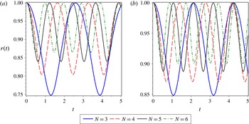
Plot of the normalized bubble radius,
 $r(t)$
, over time for either (a)
 $m=N$
(so that the polytropic index is
 $\unicode[STIX]{x1D6FE}=1$
; recall that
 $\unicode[STIX]{x1D6FE}=1$
corresponds to an isothermal bubble) or (b)
 $m=N+2$
(corresponding to a monatomic ideal gas with
 $N$
translational degrees of freedom). We also fix the scaled pressure at
 $p=1.5$
, while varying the dimension of the bubble,
 $N$
, starting with the most physically relevant case,
 $N=3$
. As the dimension increases, both the amplitude and period of the oscillation decrease. Therefore, the bubbles contract and oscillate more rapidly in higher dimensions. Identical qualitative trends are found in (b) for the monatomic ideal gas, with the amplitude and period of oscillations both decreased relative to the isothermal case shown in (a).

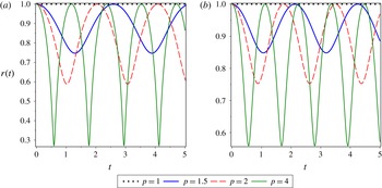
Plot of the normalized bubble radius,
 $r(t)$
, over time for fixed dimension
 $N=3$
and either (a)
 $m=N$
(so that the polytropic index is
 $\unicode[STIX]{x1D6FE}=1$
; recall that
 $\unicode[STIX]{x1D6FE}=1$
corresponds to an isothermal bubble) or (b)
 $m=N+2$
(corresponding to a monatomic ideal gas with
 $N$
translational degrees of freedom). We vary the scaled pressure
 $p$
, finding that an increase in
 $p$
results in an increase in the amplitude of the oscillations. On the other hand, an increase in the scaled pressure,
 $p$
, results in a decrease in the period of these oscillations. Therefore, as the scaled pressure increases, the bubble will oscillate more rapidly and with greater amplitude.

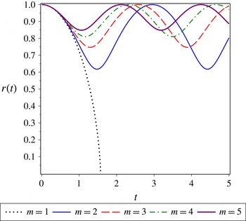
Plot of the normalized bubble radius,
 $r(t)$
, over time for fixed dimension
 $N=3$
and scaled pressure
 $p=1.5$
. We vary the parameter
 $m=N\unicode[STIX]{x1D6FE}$
, where
 $\unicode[STIX]{x1D6FE}$
is the polytropic index. For small enough
 $m$
, the bubble will collapse in finite time. For larger
 $m$
we recover bounded positive solutions which oscillate for all time. As
 $m$
is increased, the period of the oscillations decreases, so the bubbles oscillate more rapidly. The amplitude of the oscillations is also decreased as the polytropic index increases.

In figure 1 we plot the normalized bubble radius
 $r(t)$
over time for various choices of the dimension parameter,
 $N$
. Specific solutions are given for both the isothermal bubble and the bubble containing a monatomic ideal gas with
 $N$
translational degrees of freedom, although qualitative results will be similar for other choices. We find that the extent of extreme oscillations is restricted as dimension increases, with the dimension parameter
 $N$
acting to dampen the oscillations, resulting in less fluctuation in the normalized radius of the bubble over time. On the other hand, the frequency of oscillations increases (or, the period between oscillation decreases) as we increase the dimension parameter
 $N$
. Therefore, the bubbles will oscillate more quickly yet less extremely as the dimension increases. Since the normalization chosen did not depend on dimension, we have that the same qualitative results hold for the non-normalized radius
 $R(T)$
.
In figure 2 we plot the normalized bubble radius
 $r(t)$
over time for various choices of the composite scaled pressure parameter,
 $p$
. Specific solutions are again given for both the isothermal bubble and the bubble containing a monatomic ideal gas with
 $N$
translational degrees of freedom. As the parameter
 $p$
increases, the amplitude of the oscillations increases while the period of the oscillations decreases (the frequency of oscillations increases). Therefore, an increase in
 $p$
destabilizes the bubble, resulting in wilder and more rapid oscillations. Recall that
 $p\sim P_{ext}$
and
 $p^{-1}\sim P_{0}$
. Therefore, the influence of an increase in the external pressure constant
 $P_{ext}$
on the bubble radius will be qualitatively similar to an increase in the composite parameter
 $p$
, while the reverse behaviour will occur given an increase in the internal pressure constant
 $P_{0}$
. Hence, an increase in the external pressure will result in more rapid and frequent oscillations, tending to destabilize the bubble from an equilibrium state (which occurs at
 $p=1$
). On the other hand, an increase in the internal pressure coefficient has a stabilizing effect on the oscillating bubble, reducing both the amplitude and the frequency of oscillations, and can gradually push the bubble toward the equilibrium at
 $p=1$
.
We consider the influence of the scaled polytropic parameter,
 $m$
, in figure 3. Recall that
 $m=N\unicode[STIX]{x1D6FE}$
, where
 $N$
is the dimension and
 $\unicode[STIX]{x1D6FE}$
is the standard polytropic parameter. We see that (holding dimension
 $N$
fixed) an increase in
 $m$
results in a decrease in the amplitude of oscillation of the bubbles, yet an increase in the frequency at which such bubbles oscillation (i.e. the period of oscillation decreases with an increase in
 $m$
). For very small
 $m$
, the internal pressure is too weak, and so the external pressure crushes the bubble until collapse. Such small
 $m$
have been considered for gas or vapour bubbles undergoing phase change (Fuster & Montel Reference Fuster and Montel2015).
Again, figure 3 shows that when internal pressures dominate, the oscillation amplitude will be small, while when external pressures dominate, the bubble can exhibit more extreme oscillations. In the graphic provided, we take
 $N=3$
corresponding to the most physically interesting case, while we note that similar qualitative behaviours are seen at higher dimensions. The case of
 $m=3$
in figure 3 corresponds with the isothermal case, while the
 $m=5$
case corresponds to a monatomic ideal gas with
 $N$
translational degrees of freedom.
The general dynamics we see is consistent with the specific solutions considered in the papers of Klotz (Reference Klotz2013) and Kudryashov & Sinelshchikov (Reference Kudryashov and Sinelshchikov2014, Reference Kudryashov and Sinelshchikov2015).
Before concluding this section, we shall consider directly the period and oscillation of the oscillating bubble. Making use of the scaled pressure
 $p=(R(0)/R_{0})^{m}P_{ext}/P_{0}$
, we have the non-dimensional period of oscillation
 $\unicode[STIX]{x1D70F}_{\ast }$
given by the relation
 $$\begin{eqnarray}\displaystyle \unicode[STIX]{x1D70F}=\sqrt{\frac{2\unicode[STIX]{x1D70C}R_{0}^{N+4}N}{P_{0}R(0)^{m+2}(N-2)}}\unicode[STIX]{x1D70F}_{\ast }, & & \displaystyle\end{eqnarray}$$
and explicitly given by
 $$\begin{eqnarray}\displaystyle \unicode[STIX]{x1D70F}_{\ast }=\left\{\begin{array}{@{}ll@{}}\displaystyle \int _{1-2A}^{1}\left\{p(x^{-N}-1)-\frac{N}{N-m}(x^{-N}-x^{-m})\right\}^{-1/2}\text{d}x\quad & \text{for }N\neq m,\\ \displaystyle \int _{1-2A}^{1}\{p(x^{-N}-1)+Nx^{-N}\ln (x)\}^{-1/2}\text{d}x\quad & \text{for }N=m.\end{array}\right. & & \displaystyle\end{eqnarray}$$
Here, the amplitude
 $A$
of the bubble oscillation is given by the maximal root
 $0<A<1/2$
of the equation
 $$\begin{eqnarray}\displaystyle p((1-2A)^{m}-(1-2A)^{N+m})-\frac{N}{N-m}((1-2A)^{m}-(1-2A)^{N})=0 & & \displaystyle\end{eqnarray}$$
for
 $N\neq m$
, and is given exactly by
 $$\begin{eqnarray}\displaystyle A=\frac{1}{2}-\frac{1}{2}\left\{\frac{|W(-p\exp (-p))|}{p}\right\}^{1/N} & & \displaystyle\end{eqnarray}$$
for
 $N=m$
(where again
 $W$
denotes the Lambert
 $W$
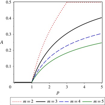
function). In figure 4 we plot the amplitude of the oscillations as a function of both the non-dimensional pressure
 $p$
and the parameter
 $m$
, for fixed
 $N=3$
. In figure 5 we similarly plot the period of the oscillations as a function of both the non-dimensional pressure
 $p$
and the parameter
 $m$
, for of both the non-dimensional pressure
 $p$
and the parameter
 $m$
, for fixed
 $N=3$
. For
 $p<1$
there are no oscillating solutions and hence
 $A=0$
. For
 $p>1$
, the amplitude of the oscillations gradually increases. For larger
 $m$
the rate of increase in the amplitude of the oscillations with
 $p$
is slower, and hence for fixed
 ${>}1$
we see a decreases in the amplitude of the oscillations as we increase
 $m$
. Note that for small
 $m$
the amplitude of the oscillations tends toward
 $A=0.5$
as
 $p$
increases. When
 $A=0.5$
, the bubble has reached the maximal (scaled) deflection from the initial radius, corresponding to
 $r(t)=0$
. Therefore, the bubble will collapse. Hence, for small
 $m$
and large enough
 $p$
, we observe bubble collapse, as expected. This is seen in figure 4 when we take
 $m=2$
and consider
 $p>3$
. For larger
 $m$
, the increase in oscillation amplitude increases more slowly, and finite time collapse of a bubble is prevented. From figure 5 we see that the non-dimensional period of oscillation,
 $\unicode[STIX]{x1D70F}_{\ast }$
, for the bubbles does not strongly depend on
 $m$
, with only a slight decrease with increasing
 $m$
for small pressures. Meanwhile, pressure has a strong influence over
 $\unicode[STIX]{x1D70F}_{\ast }$
, with a sharp decrease in
 $\unicode[STIX]{x1D70F}_{\ast }$
with pressure for small
 $p$
, and a more gradual decrease in
 $\unicode[STIX]{x1D70F}_{\ast }$
with large
 $p$
. As we take
 $p\rightarrow 1^{+}$
the period becomes arbitrarily large, as oscillating solutions do not exist for
 $p<1$
(hence any solutions which do exist would have infinite period).
Plot of the amplitude
 $A$
for oscillations of a bubble with normalized bubble radius,
 $r(t)$
, over time for fixed dimension
 $N=3$
. The solutions are plotted for various fixed
 $m=2,3,4,5$
over the non-dimensional pressure
 $p=(R(0)/R_{0})^{m}P_{ext}/P_{0}$
. For
 $0<p<1$
oscillating solutions do not exist. We see a decrease in the amplitude of oscillations as the polytropic parameter
 $m=N\unicode[STIX]{x1D6FE}$
increases.

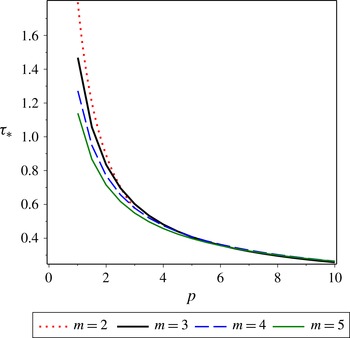
Similarly, for the case where there can be collapse of the bubble, the non-dimensional collapse time
 $T_{\ast }$
can be defined by the relation
 $$\begin{eqnarray}\displaystyle T^{\ast }=\sqrt{\frac{2\unicode[STIX]{x1D70C}R_{0}^{N+4}N}{P_{0}R(0)^{m+2}(N-2)}}T_{\ast }, & & \displaystyle\end{eqnarray}$$
and is explicitly given by
 $$\begin{eqnarray}\displaystyle T_{\ast }=\int _{0}^{1}\left\{p(x^{-N}-1)-\frac{N}{N-m}(x^{-N}-x^{-m})\right\}^{-1/2}\text{d}x. & & \displaystyle\end{eqnarray}$$
This is valid only when
 $N>m$
and
 $p>p_{crit}=N/N-m$
. In figure 6 we plot this non-dimensional collapse time as a function of the non-dimensional pressure
 $p$
and the parameter
 $m$
, for fixed
 $N=3$
. We see that the influence of
 $m$
is minimal (there is a slight increase in the collapse time as
 $m$
increases), while the more pronounced influence is due to the non-dimensional pressure
 $p$
. In particular,
 $T_{\ast }\sim 1/\sqrt{p}$
for large enough
 $p$
. This makes intuitive sense: as the ratio of external to internal pressure is increased, the bubble will collapse more rapidly.
Plot of the non-dimensional oscillation period
 $\unicode[STIX]{x1D70F}_{\ast }$
for oscillations of a bubble with normalized bubble radius,
 $r(t)$
, over time for fixed dimension
 $N=3$
. The solutions are plotted for various fixed
 $m=2,3,4,5$
over the non-dimensional pressure
 $p=(R(0)/R_{0})^{m}P_{ext}/P_{0}$
. For
 $0<p<1$
oscillating solutions do not exist, hence there is blow-up as
 $p\rightarrow 1^{+}$
. We see a decrease in the period of oscillations as the polytropic parameter
 $m=N\unicode[STIX]{x1D6FE}$
increases.

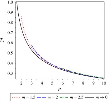
Plot of the non-dimensional collapse time,
 $T_{\ast }$
, for bubbles under the conditions
 $N>m$
and
 $p>p_{crit}=N/N-m$
. In these plots, we take the dimension to be
 $N=3$
. Similar plots can be obtained in higher dimensions. We plot the collapse times over
 $p$
, choosing values
 $m=1.5,2,2.5$
for the polytropic parameter. We find that the dominating parameter is
 $p$
, while collapse times vary little with
 $m$
. For this reason, we can take the limit
 $m\rightarrow 0$
and use the resulting exact solution for
 $T_{\ast }$
in order to obtain a qualitatively accurate approximation to the collapse time for all
 $p>p_{crit}=N/N-m$
. This approximation slightly underestimates the collapse time
 $T_{\ast }$
, and hence we conclude that the smaller the polytropic parameter,
 $m$
, the more rapid the collapse of the bubble (although this influence is relatively small). As the non-dimensional pressure
 $p$
is increased, we see a more pronounced decrease in the collapse time, finding that the collapse time decreases as
 $T_{\ast }\sim 1/\sqrt{p}$
.

Since the collapse time of the bubble appears to vary little with
 $m$
, let us take the limit
 $m\rightarrow 0$
. In this limit, the non-dimensional collapse time
 $T_{\ast }$
can be calculated exactly:
 $$\begin{eqnarray}\displaystyle \lim _{m\rightarrow 0}T_{\ast }=\frac{1}{\sqrt{p-1}}\int _{0}^{1}\frac{\text{d}x}{\sqrt{x^{-N}-1}}=\frac{1}{\sqrt{p-1}}\frac{\sqrt{\unicode[STIX]{x03C0}}}{N}\frac{\unicode[STIX]{x1D6E4}\left({\displaystyle \frac{N+2}{2N}}\right)}{\unicode[STIX]{x1D6E4}\left({\displaystyle \frac{N+1}{N}}\right)}. & & \displaystyle\end{eqnarray}$$
We take the
 $N=3$
case and plot it in figure 6. Note that this exact limiting solution is in good agreement with the results obtained for positive values of
 $m$
. Therefore, from (2.41), the collapse time of a bubble scales like
 $T_{\ast }\sim 1/\sqrt{p-1}$
when the conditions
 $N>m$
and
 $p>p_{crit}=N/N-m$
are satisfied. While such collapse solutions are only possible for
 $m<N$
(i.e.
 $\unicode[STIX]{x1D6FE}<1$
), recall that polytropic indices less than one have been considered for gas or vapour bubbles undergoing phase change (Fuster & Montel Reference Fuster and Montel2015) and therefore such collapse solutions may be physically relevant for such scenarios.
3 Solutions to the Rayleigh–Plesset equation when one or more pressure terms are zero
We now survey the possible cases where the pressure terms in (1.1) do not balance as one or both are zero. In such cases, we have either have physical behaviours (gradual decay) or non-physical behaviours (unbounded growth of the bubble), depending on the particular pressure terms which are discarded. As a special case, we recover the Rayleigh collapse time for
 $N$
dimensions as obtained in Klotz (Reference Klotz2013).
3.1 The case of
$P_{0}=0=P_{ext}$

When
 $P_{0}=0=P_{ext}$
, (1.1) reduces to
 $$\begin{eqnarray}\displaystyle R\frac{\text{d}^{2}R}{\text{d}T^{2}}+\frac{N}{2}\left(\frac{\text{d}R}{\text{d}T}\right)^{2}=0. & & \displaystyle\end{eqnarray}$$
This equation has an exact solution for any dimension
 $N$
and any initial conditions
 $R(0)$
and
 $R^{\prime }(0)$
, which is
 $$\begin{eqnarray}\displaystyle R(T)=R(0)\left\{\left(\frac{N+2}{2}\right)\frac{R^{\prime }(0)}{R(0)}T+1\right\}^{2/(N+2)}, & & \displaystyle\end{eqnarray}$$
for
 $R(0)\neq 0$
. If this solution were to be re-scaled so that
 $R(0)=0$
, we would recover equation (29) of Klotz (Reference Klotz2013). Without any balancing pressures, this bubble gradually expands or contracts in time for
 $R^{\prime }(0)\neq 0$
, with the rate of expansion when
 $R^{\prime }(0)>0$
moderated by the dimension. Meanwhile, if
 $R^{\prime }(0)<0$
, the bubble will contract until it collapses at time
 $$\begin{eqnarray}\displaystyle T^{\ast }=\frac{2R(0)}{(N+2)|R^{\prime }(0)|}. & & \displaystyle\end{eqnarray}$$
For a solution with
 $R^{\prime }(0)=0$
, we obtain a bubble of constant radius over time.
3.2 The case of
$P_{0}=0$

If
 $P_{0}=0$
yet
 $P_{ext}\neq 0$
(corresponding to an empty bubble), then (1.1) reduces to
 $$\begin{eqnarray}\displaystyle \frac{\unicode[STIX]{x1D70C}}{N-2}\left\{R\frac{\text{d}^{2}R}{\text{d}T^{2}}+\frac{N}{2}\left(\frac{\text{d}R}{\text{d}T}\right)^{2}\right\}=-P_{ext}. & & \displaystyle\end{eqnarray}$$
Note from the form of (3.4) that there can be no constant solutions. If we assume a solution has a local maximal or minimal value at
 $t=0$
so that
 $R^{\prime }(0)=0$
(with this choice of
 $R^{\prime }(0)$
motivated by the fact that we will be interested in the time from maximal radius to collapse), we obtain a first integral for (3.4) as has been done for similar cases above, and this takes the form
 $$\begin{eqnarray}\displaystyle \frac{\unicode[STIX]{x1D70C}}{N-2}R^{N}\left(\frac{\text{d}R}{\text{d}T}\right)^{2}=\frac{2P_{ext}}{N}(R(0)^{N}-R^{N}). & & \displaystyle\end{eqnarray}$$
This equation holds for positive
 $R(T)$
only if
 $R(0)\geqslant R(T)$
, and one may show that for
 $P_{ext}>0$
the solution must decrease in radius from
 $t=0$
, so manipulating this first integral gives the implicit relation between
 $R(T)$
and
 $T$
, viz.,
 $$\begin{eqnarray}\displaystyle T & = & \displaystyle \int _{R(T)}^{R(0)}\frac{x^{N/2}\,\text{d}x}{\sqrt{{\displaystyle \frac{2(N-2)P_{ext}}{\unicode[STIX]{x1D70C}N}}(R(0)^{N}-x^{N})}}\nonumber\\ \displaystyle & = & \displaystyle \sqrt{\frac{\unicode[STIX]{x1D70C}}{2P_{ext}}\frac{N}{N-2}}\int _{R(T)}^{R(0)}\left\{\left(\frac{R(0)}{x}\right)^{N}-1\right\}^{-1/2}\text{d}x.\end{eqnarray}$$
The solution will monotonically decrease in time, with eventual collapse at finite time
 $T=T^{\ast }$
given by
 $$\begin{eqnarray}\displaystyle T^{\ast } & = & \displaystyle \sqrt{\frac{\unicode[STIX]{x1D70C}}{2P_{ext}}\frac{N}{N-2}}\int _{0}^{R(0)}\left\{\left(\frac{R(0)}{x}\right)^{N}-1\right\}^{-1/2}\text{d}x\nonumber\\ \displaystyle & = & \displaystyle R(0)\sqrt{\frac{\unicode[STIX]{x1D70C}}{2P_{ext}}\frac{N}{N-2}}\int _{0}^{1}\frac{\text{d}y}{\sqrt{y^{-N}-1}}.\end{eqnarray}$$
One may verify that
 $T^{\ast }$
decreases as the dimension
 $N$
increases. Actually, noting that
 $$\begin{eqnarray}\displaystyle \int _{0}^{1}\frac{\text{d}y}{\sqrt{y^{-N}-1}}=\int _{0}^{1}\frac{y^{N/2}\,\text{d}y}{\sqrt{1-y^{N}}}=\int _{0}^{1}y^{N/2}\mathop{\sum }_{k=0}^{\infty }\frac{1\cdot 3\cdot 5\cdots (2k-1)}{2\cdot 4\cdot 6\cdots (2k)}(-y^{N})^{k}\,\text{d}y, & & \displaystyle\end{eqnarray}$$
we obtain the interesting series relation
 $$\begin{eqnarray}\displaystyle T^{\ast }=R(0)\sqrt{\frac{\unicode[STIX]{x1D70C}}{2P_{ext}}\frac{N}{N-2}}\mathop{\sum }_{k=0}^{\infty }\frac{(-1)^{k}}{\left(k+{\displaystyle \frac{1}{2}}\right)N+1}{\displaystyle \frac{1\cdot 3\cdot 5\cdots (2k-1)}{2\cdot 4\cdot 6\cdots (2k)}}. & & \displaystyle\end{eqnarray}$$
Let us also note that we may express the integral in (3.7) using gamma functions, viz.,
 $$\begin{eqnarray}\displaystyle \int _{0}^{1}\frac{y^{N/2}\,\text{d}y}{\sqrt{1-y^{N}}}={\displaystyle \frac{\sqrt{\unicode[STIX]{x03C0}}}{N}}\frac{\unicode[STIX]{x1D6E4}\left({\displaystyle \frac{1}{2}}+{\displaystyle \frac{1}{N}}\right)}{\unicode[STIX]{x1D6E4}\left(1+{\displaystyle \frac{1}{N}}\right)}, & & \displaystyle\end{eqnarray}$$
and this gives
 $$\begin{eqnarray}\displaystyle T^{\ast }=R(0)\sqrt{\frac{\unicode[STIX]{x03C0}\unicode[STIX]{x1D70C}}{2P_{ext}}\frac{1}{(N-2)N}}\frac{\unicode[STIX]{x1D6E4}\left({\displaystyle \frac{1}{2}}+{\displaystyle \frac{1}{N}}\right)}{\unicode[STIX]{x1D6E4}\left(1+{\displaystyle \frac{1}{N}}\right)}. & & \displaystyle\end{eqnarray}$$
For large
 $N$
, we have the asymptotics
 $$\begin{eqnarray}\displaystyle T^{\ast }=\unicode[STIX]{x03C0}R(0)\sqrt{\frac{\unicode[STIX]{x1D70C}}{2P_{ext}}}\left(\frac{1}{N}-\frac{2\ln (2)-1}{N^{2}}+O(N^{-3})\right). & & \displaystyle\end{eqnarray}$$
As the dimension
 $N$
increases, we see a decrease in the collapse time of the bubble. Note that this formula is exactly that obtained for the Rayleigh collapse in equation (14) of Klotz (Reference Klotz2013).
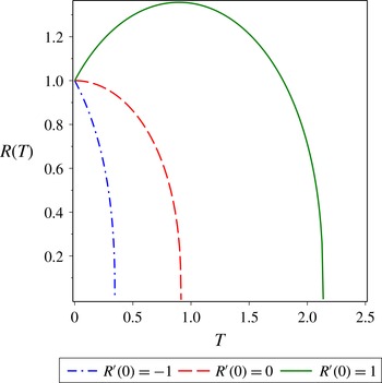
Plot of the bubble radius,
 $R(t)$
, over time for fixed dimension
 $N=3$
in the case where
 $P_{0}=0$
so that only the external pressure is acting on the bubble. This corresponds to a hollow bubble under the traditional Rayleigh dynamics. We take
 $P_{ext}/\unicode[STIX]{x1D70C}=1$
and
 $R(0)=1$
while varying the value of the initial rate of change of the radius,
 $R^{\prime }(0)$
. Naturally, the time to collapse is decreased when the bubble initially is decreasing in radius, and the time to collapse is increased if the radius is initially increasing. The plot corresponding to
 $R^{\prime }(0)=0$
corresponds to the Rayleigh collapse in equation (14) of Klotz (Reference Klotz2013).

These results show that when
 $P_{0}=0$
, the constant external forcing acts destructively on the bubble, resulting in finite time collapse. While we have taken
 $R^{\prime }(0)=0$
above, note that for
 $R^{\prime }(0)>0$
the radius will initially increase before decreasing to zero. If
 $R^{\prime }(0)<0$
, then the radius will decrease more quickly to zero. We provide numerical simulations for these scenarios in figure 7. The qualitative behaviours observed above will remain similar to those for the
 $R^{\prime }(0)=0$
case, with the exception that the quantitative time to collapse will be modified as follows. By the same approach we have used above to obtain (3.6), when
 $R^{\prime }(0)\neq 0$
we find
 $$\begin{eqnarray}\displaystyle T=\pm \int _{R(T)}^{R(0)}\frac{x^{N/2}\text{d}x}{\sqrt{R(0)^{N}(R^{\prime }(0))^{2}+{\displaystyle \frac{2(N-2)P_{ext}}{\unicode[STIX]{x1D70C}N}}(R(0)^{N}-x^{N})}}. & & \displaystyle\end{eqnarray}$$
Note that we must be careful with how we choose the
 $\pm$
root. For
 $R^{\prime }(0)<0$
, we have a solution with monotone decrease in the radius, so we shall pick the ‘
 $+$
’ root. The time to collapse for such a bubble is then
 $$\begin{eqnarray}\displaystyle T^{\ast }=\int _{0}^{R(0)}\frac{x^{N/2}\text{d}x}{\sqrt{R(0)^{N}(R^{\prime }(0))^{2}+{\displaystyle \frac{2(N-2)P_{ext}}{\unicode[STIX]{x1D70C}N}}(R(0)^{N}-x^{N})}}. & & \displaystyle\end{eqnarray}$$
Due to the appearance of the positive constant
 $R(0)^{N}(R^{\prime }(0))^{2}$
, this collapse time is less than was found for the
 $R^{\prime }(0)=0$
case in (3.7). Meanwhile, for
 $R^{\prime }(0)>0$
, the bubble first grows until it attains a maximal radius,
 $R=R_{max}$
, after which it collapses to zero radius in finite time. On the initial temporal region until the maximal radius is obtained, we take the ‘
 $-$
’ root, while on the temporal region corresponding to collapse we take the ‘
 $+$
’ root. Therefore, when
 $R^{\prime }(0)>0$
, we have the time to collapse as
 $$\begin{eqnarray}\displaystyle T^{\ast } & = & \displaystyle \int _{R(0)}^{R_{max}}{\displaystyle \frac{x^{N/2}\text{d}x}{\sqrt{R(0)^{N}(R^{\prime }(0))^{2}+{\displaystyle \frac{2(N-2)P_{ext}}{\unicode[STIX]{x1D70C}N}}(R(0)^{N}-x^{N})}}}\nonumber\\ \displaystyle & & \displaystyle +\,\int _{0}^{R_{max}}{\displaystyle \frac{x^{N/2}\text{d}x}{\sqrt{R(0)^{N}(R^{\prime }(0))^{2}+{\displaystyle \frac{2(N-2)P_{ext}}{\unicode[STIX]{x1D70C}N}}(R(0)^{N}-x^{N})}}}.\end{eqnarray}$$
Here, the maximal possible radius of the bubble,
 $R_{max}$
, can be found analytically by setting
 $R^{\prime }(T)=0$
. Doing so, the exact closed-form value of
 $R_{max}$
is found to be
 $$\begin{eqnarray}\displaystyle R_{max}=\left\{R(0)^{N}+\frac{\unicode[STIX]{x1D70C}R(0)^{N}(R^{\prime }(0))^{2}}{2P_{ext}}\frac{N}{N-2}\right\}^{1/N}=R(0)\left\{1+\frac{\unicode[STIX]{x1D70C}(R^{\prime }(0))^{2}}{2P_{ext}}\frac{N}{N-2}\right\}^{1/N}. & & \displaystyle \nonumber\\ \displaystyle & & \displaystyle\end{eqnarray}$$
The collapse times (3.14) and (3.15) constitute generalizations of the Rayleigh collapse given in equation (14) of Klotz (Reference Klotz2013) which account for various initial configurations of the bubble.
3.3 The case of
$P_{ext}=0$

In the case where the external pressure satisfies
 $P_{ext}=0$
, while
 $P_{0}\neq 0$
, one can look at the scaling of § 2, and take
 $p=0$
. If we consider
 $p=0$
in the definitions of
 $F(r)$
and
 $G(r)$
in §§2.2 and 2.3, respectively, we see that one has
 $F(r)<0$
and
 $G(r)<0$
for every
 $0<r<1$
. Since this
 $r$
represents a scaling of
 $R(T)$
such that
 $\max r(t)=1$
, there can be no oscillating solution in such cases. Therefore, when
 $P_{ext}=0$
, the solutions
 $R(T)$
do not oscillate. Furthermore, if we assume a constant solution when
 $P_{ext}=0$
, we find that (1.1) implies
 $1/R(T)=0$
, which is not possible. Hence, no constant solution can exist when
 $P_{ext}=0$
. As such, when
 $P_{ext}=0$
, the solutions can only collapse or grow in radius asymptotically.
If
 $N>m$
, we can obtain a particular solution in closed form. When
 $P_{ext}=0$
, (1.1) reduces to
 $$\begin{eqnarray}\displaystyle \frac{\unicode[STIX]{x1D70C}}{N-2}\left\{R\frac{\text{d}^{2}R}{\text{d}T^{2}}+\frac{N}{2}\left(\frac{\text{d}R}{\text{d}T}\right)^{2}\right\}=P_{0}R_{0}^{m}R^{-m}. & & \displaystyle\end{eqnarray}$$
Assuming a solution of the general form (3.2), we obtain
 $$\begin{eqnarray}\displaystyle R(T)=\left\{R(0)^{(m/2)+1}\pm \sqrt{\frac{P_{0}(N-2)}{2\unicode[STIX]{x1D70C}(N-m)}}(m+2)R_{0}^{m/2}T\right\}^{2/(2+m)}. & & \displaystyle\end{eqnarray}$$
When the ‘
 $+$
’ root is taken, the solution grows without bound, while when the ‘
 $-$
’ root is taken, the solution monotonically decreases in radius until collapse at a finite time
 $T=T^{\ast }$
given by
 $$\begin{eqnarray}\displaystyle T^{\ast }=\sqrt{\frac{2\unicode[STIX]{x1D70C}(N-m)}{P_{0}(N-2)}}\frac{R(0)^{(m/2)+1}R_{0}^{-m/2}}{m+2}. & & \displaystyle\end{eqnarray}$$
Note that this solution exists only for very specific
 $R^{\prime }(0)$
, unlike the solution (3.2) in which both
 $R(0)$
and
 $R^{\prime }(0)$
are free parameters. Therefore, the bubble collapse is a rather particular case, and we must be more careful with how we investigate this case.
In contrast to the case where
 $P_{0}=0$
yet
 $P_{ext}\neq 0$
in which the negative external forcing resulted in bubble collapse, here we have that the positive pressure will most often result in asymptotic growth of the bubble in the absence of a balancing external pressure (
 $P_{ext}=0$
). The exception is when the initial change in bubble radius is a large enough negative value, so that the small time dynamics results in collapse before the slower dynamics can kick in and increase the bubble radius.
From (3.17), we obtain
 $$\begin{eqnarray}\displaystyle \frac{\unicode[STIX]{x1D70C}}{N-2}\frac{\text{d}}{\text{d}T}\left\{R^{N}\left(\frac{\text{d}R}{\text{d}T}\right)^{2}\right\}=2P_{0}R_{0}^{m}R^{N-m-1}\frac{\text{d}R}{\text{d}T}. & & \displaystyle\end{eqnarray}$$
We may again separate variables and obtain an implicit representation for
 $R$
in terms of
 $T$
. For
 $m=N$
we get
 $$\begin{eqnarray}\displaystyle T=\pm \int _{R(0)}^{R(T)}\frac{x^{N/2}\text{d}x}{\sqrt{R(0)^{N}(R^{\prime }(0))^{2}+{\displaystyle \frac{2(N-2)P_{0}R_{0}^{N}}{\unicode[STIX]{x1D70C}}}\ln (x/R(0))}}, & & \displaystyle\end{eqnarray}$$
while for
 $m\neq N$
, we have
 $$\begin{eqnarray}\displaystyle T=\pm \int _{R(0)}^{R(T)}\frac{x^{N/2}\text{d}x}{\sqrt{R(0)^{N}(R^{\prime }(0))^{2}+{\displaystyle \frac{2P_{0}R_{0}^{N}}{\unicode[STIX]{x1D70C}}}{\displaystyle \frac{N-2}{N-m}}(x^{N-m}-R(0)^{N-m})}}. & & \displaystyle\end{eqnarray}$$
The choice of sign again will depend on whether a solution is increasing or decreasing over some interval of time. Again, if
 $R^{\prime }(0)>0$
, then the solutions will monotonically increase without bound in all cases for
 $T\geqslant 0$
. If
 $R^{\prime }(0)=0$
, the solutions will still monotonically increase without bound in all cases for
 $T>0$
. However, if
 $R^{\prime }(0)<0$
, then the solutions must initially decrease in radius, before increasing without bound. If the rate of initial decrease is strong enough in magnitude, then collapse is possible. Otherwise, the bubble will attain some minimal radius, before unbounded expansion occurs. As we shall prove below, collapse will be possible only for
 $m<N$
. In figure 8 we plot these behaviours in the sample cases of an isothermal gas (
 $m=N$
) and a monatomic ideal gas with
 $N$
translational degrees of freedom (
 $m=N+2$
).
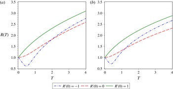
Plot of the bubble radius,
 $R(t)$
, over time for fixed dimension
 $N=3$
when (a)
 $m=N=3$
(so that the polytropic index is
 $\unicode[STIX]{x1D6FE}=1$
; recall that
 $\unicode[STIX]{x1D6FE}=1$
corresponds to an isothermal bubble) or (b)
 $m=N+2=5$
(corresponding to a monatomic ideal gas with
 $N$
translational degrees of freedom). We scale the physical quantities like
 $P_{0}/\unicode[STIX]{x1D70C}=1$
,
 $R(0)=1$
, and
 $R_{0}=1$
, while varying the initial rate of change of the bubble radius,
 $R^{\prime }(0)$
, as a control parameter. We see for
 $R^{\prime }(0)<0$
that the bubble radius initially decreases, before increasing without bound due to the lack of any external pressure to balance the gas pressure inside the bubble. On the other hand, for
 $R^{\prime }(0)\geqslant 0$
, the growth of the radius is immediate and again continues in an unbounded manner. Similar qualitative results are observed for both the isothermal (
 $m=N$
) and monatomic ideal gas with
 $N$
translational degrees of freedom (
 $m=N+2$
), with the only difference being that the decay or growth in the latter case is somewhat moderated as the pressure term is smaller in this case.

Let us assume that
 $R^{\prime }(0)<0$
so that the bubble radius initially decreases. We find that the minimal radius is given by
 $$\begin{eqnarray}\displaystyle R_{min}=R(0)\exp \left(-\frac{\unicode[STIX]{x1D70C}}{2P_{0}(N-2)}\left(\frac{R(0)}{R_{0}}\right)^{N}(R^{\prime }(0))^{2}\right) & & \displaystyle\end{eqnarray}$$
for
 $m=N$
, while when
 $m\neq N$
we must have
 $$\begin{eqnarray}\displaystyle R_{min}=R(0)\left\{1-\frac{\unicode[STIX]{x1D70C}}{2P_{0}}\left(\frac{N-m}{N-2}\right)\left(\frac{R(0)}{R_{0}}\right)^{N}(R^{\prime }(0))^{2}\right\}^{1/(N-m)} & & \displaystyle\end{eqnarray}$$
for
 $m<N$
, and
 $$\begin{eqnarray}\displaystyle R_{min}=R(0)\left\{1+\frac{\unicode[STIX]{x1D70C}}{2P_{0}}\left(\frac{m-N}{N-2}\right)\left(\frac{R(0)}{R_{0}}\right)^{N}(R^{\prime }(0))^{2}\right\}^{-1/(m-N)} & & \displaystyle\end{eqnarray}$$
for
 $m>N$
. Now, in order for a bubble to collapse in finite time, we would need
 $R_{min}\leqslant 0$
, and this is clearly only possible for
 $m<N$
. When
 $m\geqslant N$
, the bubble will decrease in size to the relevant minimal radius value given above, before then increasing in radius without bound.
The minimal value of the bubble radius in the case where
 $R^{\prime }(0)<0$
clearly depends on the value of
 $R^{\prime }(0)$
, with the value decreasing with an increase in the magnitude of
 $R^{\prime }(0)$
. Therefore, we can calculate the critical value of
 $R^{\prime }(0)$
for which the bubble will collapse rather than eventually increase in size. Since this is only possible when
 $m<N$
, we pick the corresponding formula above and set
 $R_{min}=0$
, finding that
 $$\begin{eqnarray}\displaystyle R^{\prime }(0)_{crit}=-\sqrt{\frac{2P_{0}}{\unicode[STIX]{x1D70C}}\left(\frac{R_{0}}{R(0)}\right)^{m}\frac{N-2}{N-m}}. & & \displaystyle\end{eqnarray}$$
Yet, upon taking the derivative of (3.18) and evaluating at
 $T=0$
, we find the exact same value. Hence, at the critical value
 $R^{\prime }(0)=R^{\prime }(0)_{crit}$
, the bubble collapses and the governing equation is exactly solvable. The time to collapse is again given by (3.19). When
 $R^{\prime }(0)<R^{\prime }(0)_{crit}$
, the bubble will still collapse, yet more rapidly. While such a case is not exactly solvable, we can obtain the collapse time through (3.22) by integrating from the initial radius value to a zero radius value, viz., the time of collapse is given by
 $$\begin{eqnarray}\displaystyle T^{\ast }=\int _{0}^{R(0)}\frac{x^{N/2}\text{d}x}{\sqrt{R(0)^{N}(R^{\prime }(0))^{2}+{\displaystyle \frac{2P_{0}R_{0}^{N}}{\unicode[STIX]{x1D70C}}}{\displaystyle \frac{N-2}{N-m}}(x^{N-m}-R(0)^{N-m})}}. & & \displaystyle\end{eqnarray}$$
Again, the collapse time formula (3.27) is valid only for
 $R^{\prime }(0)<R^{\prime }(0)_{crit}$
and when
 $m<N$
. For all other parameter regimes, the bubble will undergo eventual expansion.
4 Influence of surface tension and viscosity on the Rayleigh–Plesset bubble dynamics
It is possible to include surface tension and viscosity effects in (1.1). This was discussed in Prosperetti (Reference Prosperetti2004) and Klotz (Reference Klotz2013), and the resulting equation is
 $$\begin{eqnarray}\displaystyle \frac{\unicode[STIX]{x1D70C}}{N-2}\left\{R\frac{\text{d}^{2}R}{\text{d}T^{2}}+\frac{N}{2}\left(\frac{\text{d}R}{\text{d}T}\right)^{2}\right\}=P_{0}\left(\frac{R_{0}}{R}\right)^{m}-\unicode[STIX]{x1D70E}\frac{N-1}{R}-\unicode[STIX]{x1D707}\frac{2(N-1)}{R}\frac{\text{d}R}{\text{d}T}-P_{ext}, & & \displaystyle\end{eqnarray}$$
where
 $\unicode[STIX]{x1D70E}$
is the surface tension coefficient and
 $\unicode[STIX]{x1D707}$
is the viscosity coefficient. While the calculation of quantities such as surface tension and viscosity in dimensions higher than three is of course theoretical rather than experimental, and even then theoretical work in the area is lacking, there has been some work on the study of hard hyperspheres in dimensions greater than three. Finken, Schmidt & Löwen (Reference Finken, Schmidt and Löwen2001) show that the surface tension increases in value with dimension, while the work of Lue & Bishop (Reference Lue and Bishop2006) suggests that viscosity decreases with dimension in the case of hard hyperspheres.
Multiplying (4.1) by
 $R^{N-1}\text{d}R/\text{d}T$
, we can use the same approach employed elsewhere in this paper to write (4.1) in the conservation form
 $$\begin{eqnarray}\displaystyle \frac{1}{2}\frac{\unicode[STIX]{x1D70C}}{N-2}\frac{\text{d}}{\text{d}T}\left\{R^{N}\left(\frac{\text{d}R}{\text{d}T}\right)^{2}\right\} & = & \displaystyle \{P_{0}R_{0}^{m}R^{N-m-1}-P_{ext}R^{N-1}-\unicode[STIX]{x1D70E}(N-1)R^{N-2}\}\frac{\text{d}R}{\text{d}T}\nonumber\\ \displaystyle & & \displaystyle -\,2\unicode[STIX]{x1D707}(N-1)R^{N-2}\left(\frac{\text{d}R}{\text{d}T}\right)^{2}.\end{eqnarray}$$
Note that (4.2) is not integrable, due to the final term describing the effects of viscosity. Therefore, we do not expect to be able to obtain exact implicit solutions for this general equations, save for any special cases which permit serendipitous cancellations. When
 $\unicode[STIX]{x1D707}=0$
, the (4.2) still allows us to determine surface tension effects in the limit where viscus effects are negligible. Integrating this
 $\unicode[STIX]{x1D707}=0$
reduction of (4.2), we find
 $$\begin{eqnarray}\displaystyle \frac{\unicode[STIX]{x1D70C}}{N-2}R^{N}\left(\frac{\text{d}R}{\text{d}T}\right)^{2}=2\left\{\frac{P_{0}R_{0}^{m}}{N-m}R^{N-m}-\frac{P_{ext}}{N}R^{N}-\unicode[STIX]{x1D70E}R^{N-1}+K_{1}\right\} & & \displaystyle\end{eqnarray}$$
for
 $m\neq N$
, and
 $$\begin{eqnarray}\displaystyle \frac{\unicode[STIX]{x1D70C}}{N-2}R^{N}\left(\frac{\text{d}R}{\text{d}T}\right)^{2}=2\left\{P_{0}R_{0}^{m}\ln (R)-\frac{P_{ext}}{N}R^{N}-\unicode[STIX]{x1D70E}R^{N-1}+K_{2}\right\} & & \displaystyle\end{eqnarray}$$
for
 $m=N$
(the isotropic case). Here
 $K_{1}$
and
 $K_{2}$
are constants of integration. Using the (4.3)–(4.4), separating variables, and obtaining implicit solutions for the radius
 $R(T)$
, we find that
 $$\begin{eqnarray}\displaystyle T=\sqrt{\frac{\unicode[STIX]{x1D70C}}{2(N-2)}}\int _{R(T)}^{R(0)}\frac{x^{N/2}\text{d}x}{\sqrt{{\displaystyle \frac{\unicode[STIX]{x1D70C}R(0)^{N}(R^{\prime }(0))^{2}}{2(N-2)}}+J_{1}(x)}} & & \displaystyle\end{eqnarray}$$
for
 $m\neq N$
, and
 $$\begin{eqnarray}\displaystyle T=\sqrt{\frac{\unicode[STIX]{x1D70C}}{2(N-2)}}\int _{R(T)}^{R(0)}\frac{x^{N/2}\text{d}x}{\sqrt{{\displaystyle \frac{\unicode[STIX]{x1D70C}R(0)^{N}(R^{\prime }(0))^{2}}{2(N-2)}}+J_{2}(x)}} & & \displaystyle\end{eqnarray}$$
Plot of the bubble radius,
 $R(t)$
, over time for fixed dimension
 $N=3$
when (a)
 $m=N=3$
(so that the polytropic index is
 $\unicode[STIX]{x1D6FE}=1$
; recall that
 $\unicode[STIX]{x1D6FE}=1$
corresponds to an isothermal bubble) or (b)
 $m=N+2=5$
(corresponding to a monatomic ideal gas with
 $N$
translational degrees of freedom). We scale the physical quantities like
 $\unicode[STIX]{x1D70C}=1$
,
 $P_{0}=1$
,
 $P_{ext}=2$
,
 $R(0)=1$
,
 $R^{\prime }(0)=0$
and
 $R_{0}=1$
(so that
 $p=2$
in the notation of § 2), while varying the surface tension parameter,
 $\unicode[STIX]{x1D70E}$
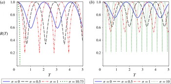
, as a control parameter. While the oscillating solutions are qualitatively similar, the larger value of
 $m$
tends to smooth the dynamics. This is most apparent for large values of the surface tension parameter, for which the
 $m=N=3$
solutions will collapse in finite time, while the
 $m=N+2=5$
solutions persist.

for
 $m=N$
, where
 $$\begin{eqnarray}\displaystyle J_{1}(x)=-\frac{P_{0}R_{0}^{m}}{N-m}(R(0)^{N-m}-x^{N-m})+\frac{P_{ext}}{N}(R(0)^{N}-x^{N})+\unicode[STIX]{x1D70E}(R(0)^{N-1}-x^{N-1}) & & \displaystyle\end{eqnarray}$$
and
 $$\begin{eqnarray}\displaystyle J_{2}(x)=-P_{0}R_{0}^{m}\ln \left(\frac{x}{R(0)}\right)+\frac{P_{ext}}{N}(R(0)^{N}-x^{N})+\unicode[STIX]{x1D70E}(R(0)^{N-1}-x^{N-1}). & & \displaystyle\end{eqnarray}$$
With this, we modify the results of §§2 and 3 in order to account for the influence of surface tension. We omit the details of this here. However, in figure 9, we plot obtained solutions over time for various values of the surface tension parameter,
 $\unicode[STIX]{x1D70E}$
. In all cases considered, an increase in the surface tension parameter,
 $\unicode[STIX]{x1D70E}$
, results in an increase in the amplitude of the bubble oscillations and an increase in the frequency of said oscillations. Therefore, increasing surface tension destabilizes the bubble dynamics. Similar qualitative results are observed for both the isothermal (
 $m=N$
) and monatomic ideal gas with
 $N$
translational degrees of freedom (
 $m=N+2$
) cases, with the only difference in the oscillating bubble dynamics being that the amplitude of oscillations in the latter case is somewhat moderated as the pressure term is in a sense damped by the larger polytropic index.
Note that the monatomic ideal gas bubble solutions (
 $m=N$
) do collapse for large enough
 $\unicode[STIX]{x1D70E}$
, with a critical value of
 $\unicode[STIX]{x1D70E}^{\ast }=10.73$
being found such that collapse occurs for
 $\unicode[STIX]{x1D70E}>\unicode[STIX]{x1D70E}^{\ast }$
. On the other hand, when
 $m=N+2$
, there is no collapse. While we plot solutions up to
 $\unicode[STIX]{x1D70E}=10$
in panel (b) of figure 9, numerical simulations up to
 $\unicode[STIX]{x1D70E}=10^{5}$
did not show collapse. Of course, there may be other parameter values which would permit this collapse. Yet this does demonstrate that the difference in collapse or persistence of the bubble is determined in many cases by the strength of the internal pressure, which acts to mitigate the influence of surface tension when
 $m$
is large enough.
Since (4.1) is not completely integrable for non-zero
 $\unicode[STIX]{x1D707}$
, to understand the influence of viscosity on the bubble dynamics we consider numerical simulations using the RKF45 method to solve the relevant initial value problem. Holding all of the parameters fixed, we provide plots of the bubble dynamics over time for various values of the viscosity parameter,
 $\unicode[STIX]{x1D707}$
, in figure 10. We include cases with non-zero surface tension parameter,
 $\unicode[STIX]{x1D70E}$
, as well, so that we can understand the bubble dynamics in the presence of both parameters.
Plot of the bubble radius,
 $R(t)$
, over time for fixed dimension
 $N=3$
when (a)
 $m=N=3$
and
 $\unicode[STIX]{x1D70E}=0$
(so that the polytropic index is
 $\unicode[STIX]{x1D6FE}=1$
; recall that
 $\unicode[STIX]{x1D6FE}=1$
corresponds to an isothermal bubble) or (b)
 $m=N+2=5$
and
 $\unicode[STIX]{x1D70E}=0$
(corresponding to a monatomic ideal gas with
 $N$
translational degrees of freedom). Plots (c) and (d) give the same physical problems as (a) and (b), respectively, with the difference being we include a surface tension parameter value of
 $\unicode[STIX]{x1D70E}=1$
. We scale the physical quantities like
 $\unicode[STIX]{x1D70C}=1$
,
 $P_{0}=1$
,
 $P_{ext}=2$
,
 $R(0)=1$
,
 $R^{\prime }(0)=0$
and
 $R_{0}=1$
(so that
 $p=2$
in the notation of § 2), while varying the viscosity parameter,
 $\unicode[STIX]{x1D707}$
, as a control parameter.

When there is no surface tension (
 $\unicode[STIX]{x1D70E}=0$
), the inclusion of the viscosity parameter
 $\unicode[STIX]{x1D707}>0$
results in a damped oscillation of the bubble. Eventually, the bubble radius will converge upon a fixed positive equilibrium value. Therefore, the inclusion of the viscous term lends greater stability to the system, and will smooth the bubble oscillations. This of course makes physical sense. In the absence of viscous dissipation (
 $\unicode[STIX]{x1D707}=0$
), the bubble was able to oscillate with constant energy. Mathematically, this corresponded to the integrability of the dynamical system (4.1). However, when we include viscous dissipation, the system will gradually lose energy, hence any oscillations cannot persist indefinitely. As such, the bubble will have to settle into an energy minimizing configuration, corresponding to a constant radius over time. This energy loss manifests mathematically in the fact that the dynamical system (4.1) is not integrable when
 $\unicode[STIX]{x1D707}>0$
, as we have discussed above.
If surface tension and viscosity terms are both included (i.e.
 $\unicode[STIX]{x1D70E}>0$
and
 $\unicode[STIX]{x1D707}>0$
), we see that for small time the surface tension term will destabilize the bubble dynamics, with the oscillation amplitude of the bubble radius increased with an increase in
 $\unicode[STIX]{x1D70E}$
, as was true in figure 9. However, as time increases, even these more extreme oscillations will be smoothed by the viscosity term, with the oscillations dissipating and the bubble settling upon a fixed positive radius for large time.
Plot of the stable equilibrium bubble radius,
 $R_{eq}$
, to which an oscillating bubble will gradually converge in the presence of viscous dissipation. We have taken
 $P_{0}=1$
,
 $R_{0}=1$
and
 $P_{ext}=2$
in (4.9). We plot the equilibrium solutions over the surface tension parameter,
 $\unicode[STIX]{x1D70E}$
, for various values of the spatial dimension parameter,
 $N$
, and the polytropic parameter,
 $m$
. When
 $m=N$
we have an isothermal bubble, while when
 $m=N+2$
we have a bubble containing a monatomic ideal gas with
 $N$
translational degrees of freedom. In all cases, an increase in the surface tension results in a decrease in this equilibrium radius. Hence, larger surface tension effects result in smaller spherical bubbles at equilibrium. On the other hand, an increase in the spatial dimension will result in larger bubbles at equilibrium. The bubbles containing a monatomic ideal gas with
 $N$
translational degrees of freedom will be larger at equilibrium than their isothermal counterparts.

We may calculate the energy minimizing configuration that the bubble must take in the large time limit. For large time, we must have
 $\text{d}R/\text{d}T\rightarrow 0$
. From the plots in figure 10, we notice that such an equilibrium radius is seemingly independent of
 $\unicode[STIX]{x1D707}$
, yet only attracts the solution when
 $\unicode[STIX]{x1D707}>0$
. The role of
 $\unicode[STIX]{x1D707}$
is more closely related to the rate at which a solution converges upon an equilibrium configuration, and the precise value of
 $\unicode[STIX]{x1D707}$
does not influence the actual structure of this equilibrium configuration. In (4.1), we see that when
 $\text{d}R/\text{d}T\rightarrow 0$
, the term involving viscosity vanishes. From (4.1), we find that the equilibrium radius
 $R=R_{eq}$
is given by a positive solution of the polynomial equation
 $$\begin{eqnarray}\displaystyle P_{0}R_{0}^{m}-\unicode[STIX]{x1D70E}(N-1)R_{eq}^{m-1}-P_{ext}R_{eq}^{m}=0. & & \displaystyle\end{eqnarray}$$
In the special case of
 $\unicode[STIX]{x1D70E}=0$
, we recover the equilibrium value given earlier in (1.3). The difference here is that, when
 $\unicode[STIX]{x1D707}>0$
, the equilibrium is attractive, and hence an initially oscillating bubble will tend to
 $R_{eq}$
as
 $T\rightarrow \infty$
. Meanwhile, in the case where
 $\unicode[STIX]{x1D707}=0$
, if we perturb an equilibrium configuration, we will obtain a solution which exhibits oscillations, as per our discussion in § 2.4. In figure 11 we provide values of the equilibrium radius
 $R_{eq}$
for various values of the surface tension and dimension of the bubble, and the results more precisely quantify what we have seen in figure 10.
4.1 Additional extensions
In addition to adding surface tension and viscosity effects, there other ways to extend the results we have presented. We list some of these extensions here.
It is natural to wonder about the utility of obtaining analytical expressions rather than simply numerically integrating the Rayleigh–Plesset equation (1.1) in order to find the bubble radius as a function of time. If one knows exactly what they are looking for, that is concerned with a very specific physical scenario which fixes all model parameters, the numerical solution would be easiest. However, the analytical solutions are useful for better understanding the possible qualitative behaviours of solutions. Such solutions are particularly useful if one is more interested in a range of parameters, rather than some fixed parameter values.
One could consider other time-dependent pressure terms. This would make the most physical sense for the external pressure term, although the internal pressure could be taken as time dependent in order to approximate thermal effects. In such cases, one would not expect the existence of first integrals as discussed in the present paper, so any results would be limited to numerical simulations or asymptotic approximations. Still, the qualitative results outlined in this paper would likely serve as a good prediction of the types of dynamics possible in the time-dependent pressure cases where the variation in time was sufficiently gradual. One could also consider variable internal pressures for the purposes of obtaining new and possibly interesting Navier–Stokes solutions.
While we have considered a bubble immersed in an incompressible fluid, it is possible to model the oscillations of a gas-filled bubble in a compressible fluid. As mentioned in Klotz (Reference Klotz2013), it should be possible to obtain a Herring equation which treats compressibility as a small damping term. See Herring (Reference Herring1941) and also the more accessible references Trilling (Reference Trilling1952) and Vokurka (Reference Vokurka1986). Prosperetti & Lezzi (Reference Prosperetti and Lezzi1986) and Lezzi & Prosperetti (Reference Lezzi and Prosperetti1987) give a systematic treatment of the subject and derive governing equations for such bubble dynamics in a compressible fluid. Prosperetti (Reference Prosperetti1987) obtains a third-order ordinary differential equation governing the bubble radius
 $R(T)$
as an analogue of (1.1) which accurately accounts for compressibility of the fluid. The analysis of such models, along the lines presented here, will be considered in a future work.
5 Conclusions
We have classified all possible pressure-driven dynamics for the Rayleigh–Plesset equation (1.1), and for its various reductions and special cases. Purely oscillating solutions to the full Rayleigh–Plesset equation are shown to exist when both pressure terms are non-zero, and we classify all possible dynamics of such solutions according to the relation involving the spatial dimension and scaled polytropic index. We find that the primary deciding factor for the existence of such solutions is the relative strength of external and internal pressure terms. When there are bubbles that oscillate for all time, we can calculate the period of oscillation for such bubbles in terms of the model parameters. When very specific parameter values are taken (in particular, specific values of the polytropic index), one may recover the results of Kudryashov & Sinelshchikov (Reference Kudryashov and Sinelshchikov2015) and earlier works. The general approach used is also valid for the isotropic case, as such a case gives logarithmic terms which were avoided in other works. In this case, we obtain oscillating and non-oscillating solutions, depending on the parameter values. Summaries of the results are given in § 2.5. From the amplitude and period expressions given there, we obtain a generalized way to understand the bubble dynamics described in some particular cases in Klotz (Reference Klotz2013), Kudryashov & Sinelshchikov (Reference Kudryashov and Sinelshchikov2014, Reference Kudryashov and Sinelshchikov2015), and earlier works.
For other regimes, the bubbles will collapse in finite time rather than oscillate for all time when the external pressures dominate, and we can calculate this collapse time as a function of the model parameters. Such results generalize the standard Rayleigh collapse time to permit internal and external pressure contributions (in addition to the generalization of the spatial dimension). Hence, we recover the Rayleigh collapse, as well as other results such as those of Klotz (Reference Klotz2013).
In order to be complete in our investigation of the possible dynamics under the pressure-driven Rayleigh–Plesset equation (1.1), we also consider various reductions of the equation accounting for cases where one or more of the internal and external pressure terms are negligible. When both pressure terms vanish, we obtain natural generalizations of the algebraic exact solutions in the literature discussed by Obreschkow et al. (Reference Obreschkow, Bruderer and Farhat2012), Klotz (Reference Klotz2013). Such algebraic solutions scale like
 $R(T)\sim (T_{c}\pm T)^{\unicode[STIX]{x1D6FC}}$
in time, where
 $\unicode[STIX]{x1D6FC}=2/N+2$
as suggested in Klotz (Reference Klotz2013), and
 $T_{c}$
is the collapse time of the bubble when the ‘
 $-$
’ solution is taken.
In the case where external pressures dominate and internal pressures can be neglected, the bubble will eventually collapse, as demonstrated in figure 7. We obtain implicit exact solutions for all cases, and from these we can calculate the time to collapse exactly. In the case
 $R^{\prime }(0)=0$
, we recover the Rayleigh-like collapse time given in equation (14) of Klotz (Reference Klotz2013), which itself is a generalization of the Rayleigh (Reference Rayleigh1917) result. If
 $R^{\prime }(0)\neq 0$
, the formula for collapse is modified, as
 $R^{\prime }(0)<0$
will hasten collapse of the bubble, while
 $R^{\prime }(0)>0$
will slow the time to collapse.
For the final case, in which internal pressures dominate and external pressures can be neglected, we find that most often the bubble will undergo continuous expansion and we may give the implicit exact solution for such cases. There is, however, a special case for which the bubble may collapse, even in the presence of dominant internal pressures. This special case corresponds to a strong initial decrease in the radius, i.e.
 $R^{\prime }(0)<R^{\prime }(0)_{crit}$
where
 $R^{\prime }(0)_{crit}<0$
is a critical threshold for the initial decrease in the radius of the bubble. For this to be valid, the dimension and polytropic parameter need to satisfy
 $m<N$
. Yet, this implies that the polytropic index
 $\unicode[STIX]{x1D6FE}$
satisfies
 $\unicode[STIX]{x1D6FE}<1$
. While a polytropic index of less than unity may seem strange physically, there is evidence that this may hold for certain applications in plasma physics. See Pudovkin et al. (Reference Pudovkin, Meister, Besser and Biernat1997) and references therein. Furthermore, it has been shown that the effective polytropic coefficient of gas or vapour bubbles undergoing phase change can be lower than unity (Fuster & Montel Reference Fuster and Montel2015).
The particular dynamics of the bubbles can be predicted in a deterministic manner and can be given solely in terms of the spatial dimension, pressures acting on the bubble and initial strain. The physically interesting bubbles either oscillate or collapse in finite time, and we can give the amplitude and period of the oscillations or the collapse time in terms of the model parameters. In the previous subsection, we also discuss the influence of both surface tension and viscosity when these terms are included in the Rayleigh–Plesset dynamics as per (4.1). We find that the inclusion of surface tension will destabilize the bubbles, resulting in more extreme oscillations, and hence collapse time can be decreased. Otherwise, the qualitative properties of the bubbles are the same as we had seen in earlier sections. In contrast, when including viscous effects, we note that the viscosity term renders (4.1) non-integrable and this term acts as a damping term. The result is that the bubbles will no longer oscillate eternally, and, rather, will tend toward a constant equilibrium radius value for large time. The value of the equilibrium radius does not depend on the value of the viscosity parameter, with the role of the viscosity parameter being to increase the rate at which the bubble tends to this equilibrium value.