

I. Introduction
Credit rating agencies (CRAs) play a key role in financial markets by assessing the credit risk of debt issuers and financial securities. However, many observers have questioned CRAs’ ability to provide reliable credit risk assessments. They argue that the issuer–pays business model, in which clients pay for their own ratings, distorts the incentives of CRAs to the extent that the fear of a loss of reputation or the fear of regulatory penalties are ineffective deterrents. Consistent with this concern, the two major CRAs, S&P and Moody’s, recently settled with the U.S. government for contributing to the financial crisis by inflating the credit ratings of residential mortgage-backed securities (RMBSs) and collateralized debt obligations (CDOs). As part of these settlements, CRAs renewed their commitment to credit rating quality.
CRAs have argued that inaccurate credit ratings were confined to securitized products and explained by their high level of complexity (Credit Rating Agencies and the Financial Crisis (2008)), and therefore, these inaccuracies do not affect other product markets. In this article, we study whether the conflicts of interest of CRAs prevail in the performance-sensitive debt (PSD) market, a much more mature and less complex market than that of securitized products. Importantly, this market allows us to go beyond the literature on the existence of credit rating inflation. The availability of pricing data, both at origination and in secondary markets, allows us to study whether market participants price the conflicts of interest of CRAs and therefore to identify if any market participant is harmed by credit rating inflation. Prior research has not yet established whether secondary market participants (such as mutual funds and pension funds, which are often less informed) are harmed by credit rating inflation. Finally, unlike the market for RMBSs and CDOs, the PSD market did not disappear after 2007. This allows us to study whether CRAs effectively changed their behavior after the settlements.
In performance-sensitive debt contracts, interest payments depend directly on a measure of the borrower’s financial health, such as credit ratings or financial ratios. Normally, if the borrower’s financial health deteriorates, the interest rate associated with the PSD loan increases.Footnote 1 In this article, we focus on the $900 billion subset of the PSD market which has interest payments that depend exclusively on credit ratings. In the context of these loans, a CRA experiences a conflict of interest when a credit rating downgrade causes an increase in the interest rate paid by the borrower (i.e., the client that pays the CRA for the credit rating). Thus, we consider the interest rate increase that would result from a credit rating downgrade as a measure of the conflicts of interest for CRAs for each loan. We then study whether this measure affects a CRA’s rating behavior, such as the probability of issuing a credit rating downgrade.
However, identifying conflicts of interest in PSD is empirically challenging. First, the decision to take a PSD loan, and simultaneously the choice of interest payment schedules, is not random. Firms can self-select into PSD either because they have positive inside information about their future prospects (Manso, Strulovici, and Tchistyi (Reference Manso, Strulovici and Tchistyi2010), Begley (Reference Begley2012)) or because they are overly optimistic (Adam, Burg, Scheinert, and Streitz (Reference Adam, Burg, Scheinert and Streitz2020)). Moreover, even within PSD contracts, it is likely that there is a bias in a naïve comparison of the probability of a downgrade between firms that chose credit rating-based PSD loans and those that did not, with the former set of firms being downgraded less frequently. Second, there is another form of selection often referred to as rating shopping (Faure-Grimaud, Peyrache, and Quesada (Reference Faure-Grimaud, Peyrache and Quesada2009), Skreta and Veldkamp (Reference Skreta and Veldkamp2009), and Sangiorgi and Spatt (Reference Sangiorgi and Spatt2017)). A firm may approach multiple CRAs and then ultimately do business with the CRA that offers the most favorable credit rating. As a result, credit ratings are inflated not due to CRAs yielding to conflicts of interest but rather due to unintentional errors inherent in the credit rating process.
Our empirical setting allows us to mitigate these concerns. First, the ability to observe credit ratings through time allows us to exploit time-series variation within borrowers, effectively controlling for time-invariant characteristics of firms that may affect the choice of PSD contract and subsequent credit rating downgrades. Moreover, our data also allow us to include loan fixed effects in many of our tests. Since interest rate schedules are determined at loan origination, exploiting variation in the cost of downgrades across time and within loan contracts mitigates selection concerns. Second, the richness of the data allows us to account for time-varying firm-level factors such as borrower quality and managerial optimism, as well as various dimensions of loan contracts that are determined at origination.Footnote 2
We start by investigating the relationship between the probability that a borrower is downgraded by a CRA and the increase in borrowing costs that would result from a downgrade. If CRAs internalize the additional cost to their client, a higher cost of a downgrade should be associated with a lower probability of a downgrade. Consistent with this proposition, we find that a one standard deviation increase in the cost of a downgrade is associated with a decreased downgrade likelihood of about 0.67 percentage points (pp) per quarter, which is a 26% reduction relative to the unconditional mean. This result is robust to a wide range of regression specifications (including the inclusion of loan fixed effects), to multiple measures of the cost of a downgrade, and to analyzing the downgrades by S&P and Moody’s separately. We also show that, conditional on downgrading, CRAs are slower to downgrade their clients when the downgrade is more costly. Importantly, our analysis draws inferences from within-borrower–CRA relationships over time (i.e., from downgrades that occur after origination). This is inconsistent with borrowers rating shopping or self-selecting into PSD loans.
Next, we further refine our empirical strategy by exploiting variation in the relevance of each CRA’s rating. When a CRA’s rating is decisive for setting borrowing costs—either because it is the only rating or because it is the better rating—the CRA is significantly less likely to issue a downgrade. This reluctance is particularly pronounced for clients that are potentially more profitable. Moreover, we show that loans approaching maturity are also less likely to be downgraded. Overall, our findings are consistent with the proposition that CRAs yield to conflicts of interest that result from the issuer–pays business model of credit ratings.
One potential challenge to our interpretation of our results is that they could be driven by firms hiding negative financial information from CRAs rather than by CRAs catering to their clients. CRAs issue credit ratings based on the information reported by firms without conducting independent audits, and firms whose borrowing costs would experience a larger increase in the eventuality of a downgrade might be more likely to hide negative information. We exploit a dramatic drop in commodity prices as a highly visible negative shock to the creditworthiness of a subset of firms in our sample. We show that CRAs yield to conflicts of interest even in this setting, where affected firms arguably had little room to hide the negative information.Footnote 3
Another potential challenge to our interpretation of our results is that our results may be driven by loans associated with firms that are close to losing their investment grade classification. CRAs could have implicit approval from investors to inflate credit ratings for those firms because the loss of an investment grade classification could translate not only to increased borrowing costs and a lower future availability of funding for firms but also to reduced investment opportunities for investors due to regulatory restrictions (Bruno, Cornaggia, and Cornaggia (Reference Bruno, Cornaggia and Cornaggia2016)). Inconsistent with this concern, we show that our results hold for borrowers irrespective of their initial rating. We note that this result is also inconsistent with our results being explained by CRAs internalizing the potential negative effects of downgrades on firms’ subsequent access to credit, since these effects should be most prevalent for firms that are close to losing their investment grade classification. We further mitigate the concern that our results are driven by CRAs internalizing negative externalities to the firms they downgrade with empirical tests based on credit rating reversals, by showing that CRAs internalize the positive externalities of credit rating upgrades, and by analyzing downgrades and upgrades jointly using an ordered logit framework.
Next, we consider the possibility that our results are explained by firms with higher cost of downgrade being more aggressive in decreasing leverage when they perceive that their likelihood of experiencing a credit rating downgrade is high. Inconsistent with this concern, we show that there is no relationship between a firm’s cost of downgrade and its debt issuance activities.
Lastly, we consider the possibility that our results are explained by managers with positive inside information about future firm performance selecting into contracts with higher cost of downgrade. We mitigate this concern in multiple ways. First, we show that our results hold even when excluding the first 2 years of the loans’ lives. Since the value of inside information decays rapidly as information is revealed, this result is inconsistent with managers’ optimism driving our results. Second, we proxy for CEO optimism using measures based on option holdings and find no indication that positive insider information is responsible for our findings. Furthermore, our results hold in regressions that exploit variation within loans (i.e., after all loan contract parameters have been set). Finally, we show that firms with higher cost of downgrade do not subsequently outperform their counterparts.Footnote 4
All of our tests are consistent with the proposition that CRAs cater to the firms that pay them. While we recognize that it is possible to propose an alternative explanation for each one of our tests in isolation, it seems improbable that there is an alternative explanation consistent with the multiple tests.
We then investigate whether market participants price the conflicts of interest of CRAs or whether they are harmed by these conflicts. We first focus on well-informed market participants (e.g., the initial lenders). We find that a one standard deviation increase in the average cost of downgrade is associated with a 6% increase in interest spreads relative to the unconditional mean. This is consistent with lenders being (to some extent) aware of the conflicts of interest of CRAs and pricing them in the PSD market.
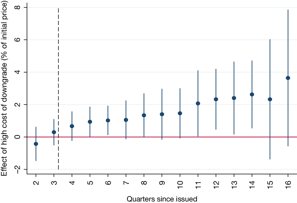
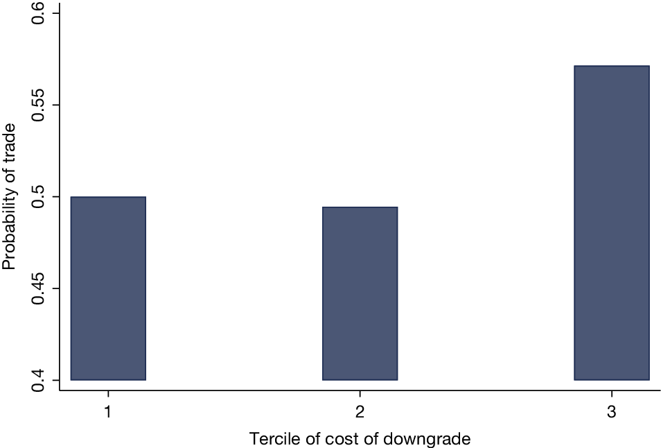
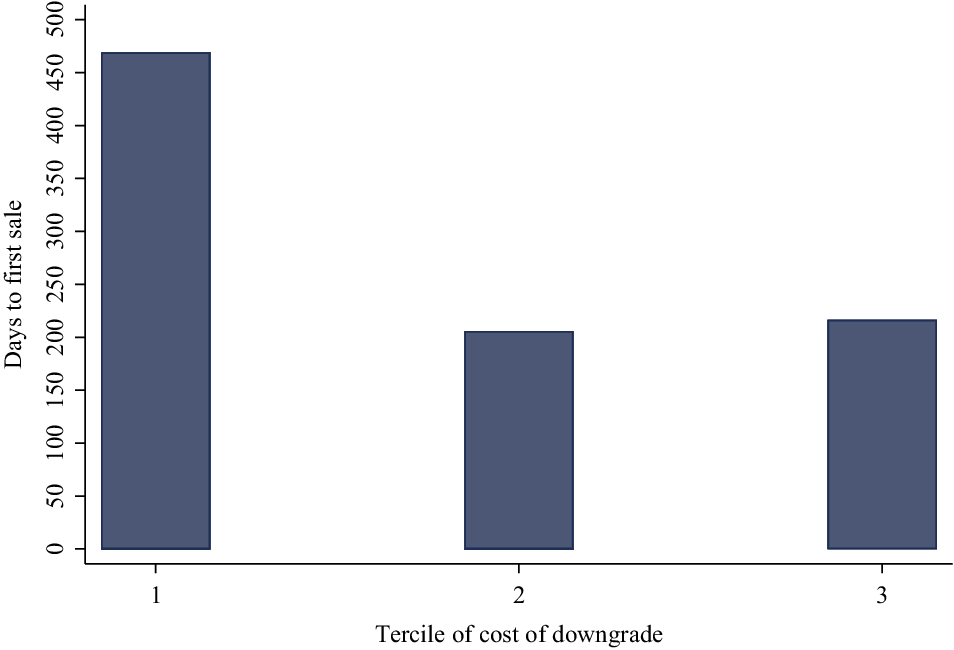
Next, we focus on the secondary market. Investors such as mutual funds and loan funds tend to be less informed than banks. Thus, it is possible that these investors do not internalize the conflicts of interest of CRAs. Consistent with this proposition, we find a significant decrease in the yield premiums associated with high cost of downgrade loans 1 year after loan origination. Moreover, this decrease in premiums persists through the remainder of the loan’s life. In addition, we document that originating banks are more likely to sell loans with high costs of downgrade and that among the loans they sell, loans with high cost of downgrade are sold faster.
Recently, CRAs have been accused of similar catering behavior in the market for RMBSs and CDOs. This behavior contributed to the financial crisis (Griffin (Reference Griffin2019)) and resulted in large settlements between the two major CRAs and the Department of Justice (DOJ). Importantly, the lawsuits and the subsequent settlements were intended not only to punish past misbehavior but also to improve future CRA conduct. In fact, as part of their respective settlements, both CRAs renewed their commitment to credit rating quality and affirmed the importance of credit ratings being impartial and not driven by business concerns. We test whether the relationship between the probability of a downgrade and the cost of a downgrade weakens after the settlements and find no evidence of a weakened relationship. Moreover, CRAs might have adjusted their behavior shortly after the 2008 financial crisis (i.e., before the settlements) due to potential litigation threats. However, inconsistent with this explanation, we find that their catering behavior remained largely stable from 2001 to 2016. Overall, these results suggest that the settlements did not have the intended effect of improving credit rating quality and curbing CRA behavior, at least in the PSD market.
This article relates to a recent literature on CRA behavior in the market for securitized products and its role in the financial crisis. Griffin and Tang (Reference Griffin and Tang2012) show that CRAs adjusted the ratings of securitized products to benefit clients at the expense of investors. Griffin, Nickerson, and Tang (Reference Griffin, Nickerson and Tang2013) show that CRAs inflated credit ratings beyond their models when facing competition. He, Qian, and Strahan (Reference He, Qian and Strahan2011), (Reference He, Qian and Strahan2012) and Efing and Hau (Reference Efing and Hau2015) show that CRAs issued increasingly optimistic credit ratings for asset-backed securities (ABSs) structured by large clients that provided them with more business. These positive credit ratings benefitted CRAs’ clients through higher prices for their securities (Ashcraft, Goldsmith-Pinkham, Hull, and Vickery (Reference Ashcraft, Goldsmith-Pinkham, Hull and Vickery2011)). Our article shows that, despite claims by CRAs to the contrary, credit rating inflation is not limited to structured products but is also a feature of loan markets and that credit rating inflation continued after CRAs settled with the government postcrisis.
This article also relates to the literature that studies the conflicts of interest of CRAs more generally. Opp, Opp, and Harris (Reference Opp, Opp and Harris2013) show that credit rating inflation can be induced by regulatory reliance on the credit ratings themselves. Mathis, McAndrews, and Rochet (Reference Mathis, McAndrews and Rochet2009) and Bolton, Freixas, and Shapiro (Reference Bolton, Freixas and Shapiro2012) develop models in which reputation is not always a sufficient deterrent to prevent CRAs from catering to clients.Footnote 5 In the case of corporate bonds, Becker and Milbourn (Reference Becker and Milbourn2011) show that increased competition from Fitch lowered the credit rating quality of S&P and Moody’s.Footnote 6 In contemporaneous work, Cornaggia, Cornaggia, and Israelsen (Reference Cornaggia, Cornaggia and Israelsen2023) show credit rating inflation in the municipal bond market.
In our setting of PSD loans, prior work compares firms with credit rating-based loans to firms with accounting ratio-based loans. These articles show that firms with credit rating-based loans experience fewer credit rating downgrades (Kraft (Reference Kraft2015)) and more credit rating upgrades (Bannier and Wiemann (Reference Bannier and Wiemann2011)), but they are largely silent on causality. Our article complements this work in multiple ways. First, we show evidence of CRA catering in the PSD market after accounting for selection concerns.Footnote 7 Second, we show that this catering behavior remains prevalent postcrisis, which suggests that government settlements are insufficient deterrents. Third, we show that lenders are aware of and price the conflicts of interest of CRAs. In contrast, secondary market participants seem to be less aware of these conflicts, which suggests that the least informed investors are the most harmed by credit rating inflation.
Finally, this article contributes to the literature that focuses on understanding the use and the implications of PSD loans. Asquith, Beatty, and Weber (Reference Asquith, Beatty and Weber2005) show that PSD loans can prevent agency conflicts and costly re-negotiations. Tchistyi, Yermack, and Yun (Reference Tchistyi, Yermack and Yun2011) show that PSD loans allow managers to gain private benefits at the expense of firm risk.Footnote 8
II. Background
A. Performance-Sensitive Debt
Performance-sensitive debt (PSD) is a type of debt in which interest payments depend on a measure of a borrower’s financial health (e.g., credit ratings, debt-to-cash flow ratio). The idea behind this type of debt obligation is to delay the costly renegotiation that results from borrowers violating covenants. In general, if a borrower’s financial health deteriorates, the interest rate associated with the PSD obligation increases, thus compensating the debt holder for the additional risk.
PSD contracts became common in the early 1990s. Now, the total size of the PSD market is over $2 trillion. In this article, we focus on the $900 billion market in which interest payments depend exclusively on credit ratings.
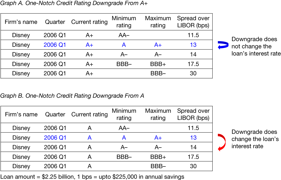
In PSD contracts, interest rates are contractually linked to measures of a borrower’s financial health through a pricing grid. Figure 1 shows the pricing grid from The Walt Disney Co.’s syndicated 5.25-year revolving credit facility issued on Feb. 23, 2005. The loan amount was $2.25 billion. The facility’s pricing grid indicates that The Walt Disney Co. can be subject to pay five different interest rates, depending on its long-term senior debt rating. For example, if the firm’s credit rating by S&P is AA- or better, then The Walt Disney Co. is subject to an interest rate of 11.5 bp over the London Interbank Offered Rate (LIBOR). If their credit rating is between A and A+, the interest rate increases to 13 bp over LIBOR. The highest interest rate that The Walt Disney Co. may be required to pay under this facility is 30.0 bp over LIBOR, which is an increase triggered by a credit rating deterioration to BBB- or worse.
Figure 1 shows the pricing grid from The Walt Disney Co.’s syndicated 5.25-year revolving credit facility issued on Feb. 23, 2005. Graph A shows that there is no change in the loan’s interest rate if the firm’s credit rating changes from A+ to A. Graph B shows that the loan’s interest rate changes from LIBOR +13 bps to LIBOR +14 bps if the firm’s credit rating changes from A to A−. The 1 bps increase translates into additional borrowing costs of as high of $225,000 per year.

FIGURE 1 Long description
The figure contains two tables and a footer note.
Graph A. One-Notch Credit Rating Downgrade From A plus.
The table has six columns: Firm's name (Disney), Quarter (2006 Q 1), Current rating (A plus), Minimum rating, Maximum rating, and Spread over L I B O R (b p s).
* Row 1: Minimum AA minus, Spread 11.5.
* Row 2 (highlighted in blue): Minimum A, Maximum A plus, Spread 13.
* Row 3: Minimum A minus, Maximum A minus, Spread 14.
* Row 4: Minimum BBB minus, Maximum BBB plus, Spread 17.5.
* Row 5: Maximum BBB minus, Spread 30.
A blue U-shaped arrow to the right of rows 2 and 3 points back to row 2 with the text: Downgrade does not change the loan's interest rate.
Graph B. One-Notch Credit Rating Downgrade From A.
The table structure is identical but the Current rating is A.
* Row 1: Minimum AA minus, Spread 11.5.
* Row 2 (highlighted in blue): Minimum A, Maximum A plus, Spread 13.
* Row 3: Minimum A minus, Maximum A minus, Spread 14.
* Row 4: Minimum BBB minus, Maximum BBB plus, Spread 17.5.
* Row 5: Maximum BBB minus, Spread 30.
A red curved arrow to the right points from row 2 down to row 3 with the text: Downgrade does change the loan's interest rate.
Footer note: Loan amount = $2.25 billion, 1 b p s = up to $225,000 in annual savings.
B. Credit Rating Agencies and Conflicts of Interest
The main role of CRAs is to perform a continual assessment of firms’ creditworthiness. CRAs communicate these assessments to financial markets in the form of credit ratings. Credit ratings are important for the rated firm because they affect the firm’s ability to access capital through the value placed on them by investors, either for informational or regulatory reasons. Importantly, it is not the investor who pays for the issuance of the credit rating but rather the rated firm itself. This issuer–pays business model of credit ratings has been subject to extensive criticism because it can generate a conflict of interest that can lead to CRAs catering to the firms that pay them.
In our setting of credit rating-based PSD loans, this conflict arises when a credit rating downgrade by a CRA causes a change in the pricing schedule that increases the interest rate paid by the borrower. For example, in the pricing grid from Figure 1, there is no change in Disney’s borrowing costs (i.e., the interest rate would remain 13 bp over LIBOR) if the firm is downgraded from a credit rating of A+ to a credit rating of A. However, if the firm is downgraded to A−, its borrowing costs would increase to 14 bp over LIBOR, implying additional annual interest expenses of up to approximately $225,000 if the entire credit facility were drawn. This number is about half the median annual cost of a downgrade in our sample (i.e., $520,000). We hypothesize that, all else being equal, a CRA will be more reluctant to downgrade a firm if the downgrade causes higher costs for the borrower. Moreover, the misalignment of incentives should be even more severe when a CRA’s rating is the one that leads directly to an increase in borrowing costs.
Credit ratings are supposed to be an objective and high-quality assessment of borrower creditworthiness. CRAs claim to meet the highest standards of integrity, independence, objectivity, and transparency (U.S. Securities and Exchange Commission (2002)). CRAs are aware that credit ratings can negatively affect borrowers’ funding costs (Moody’s Investors Service (2002)). However, CRAs’ guidelines are explicit in that credit ratings are issued independently of the effect that they may have on the borrower (U.S. Securities and Exchange Commission (2002), S&P Global Ratings (2018)). Similarly, CRAs acknowledge the conflicts of interest that arise from the issuer–pays business model (Department of Justice (2015), (2017)). However, fear of diminished reputation and regulatory penalties is often thought to mitigate these conflicts. Section C of the Supplementary Material includes excerpts from CRA documents, regulator documents, congressional hearings, DOJ press releases, and settlement statements of facts discussing these issues.
CRAs catered to underwriting banks by inflating the credit ratings associated with RMBSs and CDOs, making them important contributors to the financial crisis (Griffin et al. (Reference Griffin, Nickerson and Tang2013)). Recently, both S&P and Moody’s agreed to settlements with the DOJ in which they i) explicitly acknowledged failing to adhere to their own standards when rating securitized products and ii) renewed their commitment to credit rating quality (see Section C of the Supplementary Material).
The catering behavior of CRAs during the run-up to the financial crisis has partly been attributed to the complexity of securitized products (Griffin (Reference Griffin2019)). In this article, we study whether the conflicts of interest affecting CRAs prevail in other less complex markets, such as the PSD market. Importantly, pricing data are more reliable and available for PSD loans than for RMBSs and CDOs, which makes the PSD setting ideal for studying whether market participants recognize and internalize the conflicts of interest, both at origination and in the secondary market. Finally, we also study whether the DOJ settlements were effective in holding CRAs to their renewed commitment to credit rating quality, a question that cannot be answered by studying the RMBS and CDO markets because those markets disappeared before the settlements.
III. Data, Sample Selection, and Empirical Framework
A. Primary Data
We obtain loan-level data on performance pricing (i.e., pricing grids) from LPC DealScan. Recall that we focus on loans with performance provisions that depend exclusively on senior credit ratings. To identify where borrowers stand in the pricing grid, we assign to each loan the corresponding borrower’s long-term senior unsecured credit rating from Bloomberg.Footnote 9 We consider the credit ratings issued by S&P and Moody’s. Following Tchistyi et al. (Reference Tchistyi, Yermack and Yun2011), for cases in which borrowers have received credit ratings from both CRAs, we consider the better of the two ratings as relevant for pricing purposes.
We then use the pricing grids to assign each loan in each quarter the current interest spread and the interest spread that would prevail after a credit rating downgrade. Some contracts give borrowers a choice between different types of reference rates for determining interest spreads (e.g., LIBOR, the bank’s prime rate). Since interest spreads over LIBOR are by far the most common, we use this market rate as our baseline measure for interest spreads.Footnote 10 We use
$ cost\hskip0.35em of downgrade $
 to refer to the difference between the spread at the prevailing credit rating and the spread at the credit rating one notch below it.
B. Secondary Data and Final Sample
Initially, we obtain pricing grid data for 31,005 facilities originated between 2000 and 2016. We link these facilities to Compustat using the latest DealScan-Compustat linking table (Chava and Roberts (Reference Chava and Roberts2008)), which leaves 27,141 loans. We then require all relevant loan and firm information to be nonmissing, which leaves 3,700 loans. Of these loans, 2,075 have pricing grids that depend exclusively on credit ratings. Finally, we require borrowers to have credit ratings issued by S&P or Moody’s.Footnote 11 The final sample consists of 1,988 loans spanning 22,760 loan-quarter observations.Footnote 12 The sample consists of 510 distinct borrowers, of which 415 obtain at least two loans, with an average of 4.1 loans per borrower. Among these, 387 firms have overlapping loans, meaning that they hold more than one loan outstanding at the same time during the sample period.
Panels A and B of Table 1 describe the final sample. The mean increase in borrowing costs following a one-notch downgrade is 13.7 bp, with an interdecile range of 25 bp. Moreover, the cost of downgrade is nonzero 80% of the time. Downgrades are rare: The likelihood of a borrower being downgraded in a given quarter is, on average, only 2.6%. The median credit rating throughout the sample is BBB. The average loan size is $914.0 million, 80% of loans are revolvers, and conditional on being downgraded, the average borrower is downgraded within 4.8 quarters of issuing a loan. The Appendix describes these and the remaining variables used in the article and specifies the numerical equivalence assigned to each credit rating (e.g., AAA/Aaa = 1, AA+/Aa1 = 2, AA/Aa = 3).

TABLE 1 Long description
The table is divided into three sections.
Panel A. Borrower-Quarter Characteristics (N = 22,760 for most rows):
* Cost of downgrade (bps): Mean 13.74, Std. Dev. 12.07, p10 0.00, p50 12.50, p90 25.00.
* Leverage: Mean 0.31, Std. Dev. 0.17, p10 0.12, p50 0.30, p90 0.51.
* Total assets ($ billion): Mean 23.42, Std. Dev. 56.15, p10 2.08, p50 8.81, p90 47.02.
* Intangibles over assets: Mean 0.21, Std. Dev. 0.20, p10 0.00, p50 0.14, p90 0.55.
* Profitability (R O A): Mean 0.01, Std. Dev. 0.02, p10 -0.00, p50 0.01, p90 0.03.
* 1(downgrade) (percent): Mean 2.57, Std. Dev. 15.81, p10 0.00, p50 0.00, p90 0.00.
* Issuer credit rating (numeric): Mean 9.16, Std. Dev. 2.63, p10 6.00, p50 9.00, p90 12.00.
* R & D ($ million, N = 10,401): Mean 283.81, Std. Dev. 620.20, p10 0.00, p50 65.92, p90 718.10.
Panel B. Loan Characteristics (N = 1,988 for most rows):
* No. of financial covenants: Mean 1.46, Std. Dev. 0.83, p10 0.00, p50 1.00, p90 2.00.
* Loan amount ($ million): Mean 914.04, Std. Dev. 910.40, p10 150.00, p50 550.00, p90 2200.00.
* 1(secured): Mean 0.16, Std. Dev. 0.37, p10 0.00, p50 0.00, p90 1.00.
* Average cost of downgrade: Mean 14.82, Std. Dev. 8.50, p10 6.83, p50 12.50, p90 25.00.
* 1(revolver): Mean 0.80, Std. Dev. 0.40, p10 0, p50 1, p90 1.
* Time to downgrade (quarters, N = 455): Mean 4.77, Std. Dev. 5.14, p10 0.00, p50 3.00, p90 12.00.
Panel C. Variation Within Groups (N = 22,760):
* 1(downgrade) (percent): Overall Std. Dev. 15.81, Within Credit Rating 15.59, Within Firm 15.03, Within Year 15.76.
* Cost of downgrade (bps): Overall Std. Dev. 12.07, Within Credit Rating 10.94, Within Firm 8.84, Within Year 11.90.
* Time to downgrade (quarters): Overall Std. Dev. 4.39, Within Credit Rating 4.30, Within Firm 3.56, Within Year 4.17.
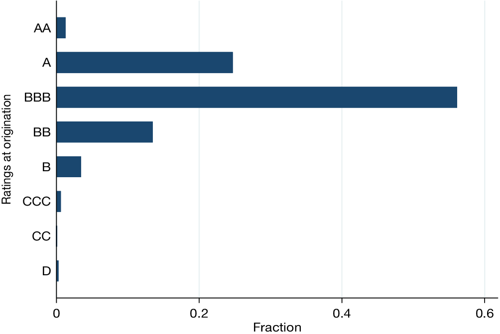
Finally, Figure 2 shows the distribution of credit ratings at origination. The most common rating is BBB, followed by AA. Overall, 93% of observations are rated at or above investment grade.
Figure 2 shows the distribution of credit ratings at the time of loan origination for our sample of credit rating-based PSD loans. The credit rating scale is simplified by combining the credit ratings within each letter credit rating category. For example, we combine the initial credit ratings of A+, A, and A− into one group, A.

FIGURE 2 Long description
The Y-axis is labeled Ratings at origination and lists categories from top to bottom: A A, A, B B B, B B, B, C C C, C C, and D. The X-axis is labeled Fraction and ranges from 0 to 0.6 in increments of 0.2.
* A A: A very short bar near 0.01.
* A: A bar extending to approximately 0.25.
* B B B: The longest bar, extending to approximately 0.56.
* B B: A bar extending to approximately 0.13.
* B: A short bar extending to approximately 0.03.
* C C C: A negligible bar near 0.005.
* C C: A negligible bar near 0.
* D: A negligible bar near 0.
The distribution is heavily concentrated in the investment-grade B B B and A categories, with a significant drop-off for ratings below B B.
C. Empirical Framework
Pricing grids vary within loan contracts (and therefore the change in borrowing costs associated with a credit rating downgrade also varies). Thus, to study whether the conflicts of interest of CRAs affect the credit ratings they issue, we estimate specifications of the form

where
$ 1{(downgrade)}_{i,t} $
 is an indicator that takes the value of 1 if borrower
$ i $
 is downgraded in quarter
$ t $
 , and 0 otherwise. The independent variable of interest is
$ cost\hskip0.35em of\hskip0.1em {downgrade}_{i,l,t} $
 , a measure of the increase in the loan spread that would result from a one-increment credit rating downgrade for loan
$ l $
 in quarter
$ t $
 . Thus, this variable captures the time-varying degree of the CRAs’ conflicts of interest for each loan. The higher the increase in a firm’s borrowing costs following a one-notch downgrade, the stronger the incentive for the CRA to avoid the downgrade. The variable
$ {X}_{i,l,t} $
 is a vector of time-varying loan- and firm-level characteristics and fixed effects. In secondary tests, we also estimate specifications in which the dependent variable is the time interval in which the firm is downgraded after loan origination.
Identifying conflicts of interest in PSD is challenging for multiple reasons. First, firms could self-select into PSD either because they have inside information (Manso et al. (Reference Manso, Strulovici and Tchistyi2010), Begley (Reference Begley2012)) or because they are overly optimistic (Adam et al. (Reference Adam, Burg, Scheinert and Streitz2020)). Even within PSD contracts, a naïve comparison of the probability of a downgrade between firms that self-selected into ratings-based PSD and those that did not is likely to be biased, with the former set of firms being downgraded less frequently. Consistent with this concern, Table 2 shows that firms with credit rating-based PSD loans differ significantly from those with accounting ratio-based PSD loans across a range of observable characteristics. Firms with credit rating-based PSD loans tend to be larger, less leveraged, and more likely to rely on larger, unsecured loans compared to firms whose PSD terms are based on accounting ratios.

TABLE 2 Long description
The table consists of four columns: Metric, Accounting Ratio-Based Mean, Credit Rating-Based Mean, and Difference.
* Leverage: 0.41 vs 0.31, difference 0.10.
* Total assets in dollars billions: 4.92 vs 23.42, difference minus 18.50.
* Intangibles over assets: 0.29 vs 0.21, difference 0.09.
* Profitability R O A: 0.005 vs 0.009, difference minus 0.004.
* R and D in dollars millions: 61.53 vs 283.80, difference minus 220.96.
* Number of financial covenants: 2.12 vs 1.52, difference 1.24.
* Loan amount in dollars millions: 350.9 vs 894.5, difference minus 543.64.
* 1 secured: 0.88 vs 0.18, difference 0.70.
* Cost of one grid in rating or ratio, b p: 18.36 vs 13.74, difference 4.63.
* Number of observations: 21,789 for Accounting Ratio-Based, 22,760 for Credit Rating-Based, totaling 44,549.
Statistical significance is indicated by asterisks on the difference values.
Second, there is another type of selection often referred to as rating shopping. A firm may approach a number of CRAs and then choose to do business with the agency that offers the most positive credit rating.Footnote 13 As a result, credit ratings are overly optimistic due to the unintentional errors inherent in the credit rating process rather than CRAs yielding to conflicts of interest.
Our empirical setting allows us to mitigate both of these selection concerns. Since both selection concerns are borrower-specific, we include borrower (i.e., firm) fixed effects in all specifications, effectively exploiting within-borrower variation in the impact of a credit rating downgrade on loan spreads. However, other variables likely correlated with downgrade likelihood (e.g., borrower quality, managerial optimism) are time-varying, so they are not accounted for by the borrower fixed effects. Thus, we include time-varying variables of financial health in
$ {X}_{i,l,t} $
 , such as the firm’s current credit rating, size (measured by the log of total assets), profitability, asset tangibility, and leverage.
In addition, because the probability of a credit rating downgrade varies with the business cycle (Bar-Isaac and Shapiro (Reference Bar-Isaac and Shapiro2013)), we include year–quarter fixed effects in
$ {X}_{i,l,t} $
 .Footnote 14 We also control for loan-level characteristics that are jointly determined at origination, including loan amount, number of financial covenants, whether the loan is secured, loan type (e.g., revolver or term loan), and deal purpose. Finally, in Section IV.C, we estimate a more stringent specification that includes loan fixed effects.Footnote 15
D. Sources of Variation
The most stringent specification in our initial analysis includes fixed effects for the current credit rating, borrower, and year–quarter. Thus, we exploit variation in credit rating downgrade probabilities and in borrowing costs from three separate sources. That is, we exploit variation in these variables i) across loans and across time within credit ratings, ii) across loans and across time within borrower, and iii) across loans within time. In this section, we show that, even with these tight sets of fixed effects, there is enough variation in the data to identify the effects of CRAs’ conflicts of interest in PSD.
Panel C of Table 1 shows within-group standard deviations of the dependent and independent variables that are most relevant to our regressions. The within-credit rating standard deviation of
$ 1(downgrade) $
 is 15.6 pp, which is very similar to its overall standard deviation of 15.8 pp. Similarly, the within-credit rating standard deviation of
$ cost\hskip0.35em of downgrade $
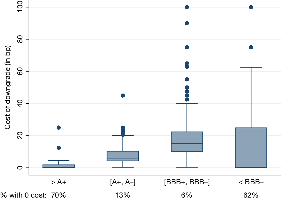
 is 10.9 bp (compared to 12.1 bp overall). Figure 3 shows the distribution of the cost of a one-notch downgrade by credit rating category at origination. Borrowers rated above A+ or below BBB− exhibit a high incidence of zero downgrade costs. In contrast, firms rated between A+ and BBB− face downgrade costs more frequently and show greater variation in these costs.
Figure 3 shows the distribution of the cost of a one-notch credit rating downgrade across the different credit rating groups (at origination). The bottom row tabulates the fraction of observations within each credit rating group that have a cost of downgrade of zero.

FIGURE 3 Long description
The Y axis is labeled Cost of downgrade (in b p) with a scale from 0 to 100. The X axis contains four credit rating groups. From left to right, the data shows:
* Greater than A plus: The box is very low, near 0. The percentage with 0 cost is 70 percent. There are two outliers near 12 and 25 b p.
* Bracket A plus, A minus bracket: The box ranges from approximately 5 to 10 b p with a median around 6. The percentage with 0 cost is 13 percent. Several outliers extend up to 45 b p.
* Bracket B B B plus, B B B minus bracket: The box ranges from approximately 10 to 22 b p with a median around 15. The percentage with 0 cost is 6 percent. Numerous outliers are clustered between 40 and 100 b p.
* Less than B B B minus: The box is larger, ranging from 0 to 25 b p. The percentage with 0 cost is 62 percent. Outliers are present at 75 and 100 b p.
Panel C of Table 1 also shows that the time required for the firm to be downgraded follows the same pattern as downgrades and the cost of a downgrade and that there is significant variation in the previous three variables within firm and within year. Overall, there is more than sufficient variation in the data to expect that our specifications will have power.
IV. Credit Rating Agency Behavior and the Cost of Downgrades
We start by investigating whether CRAs are less likely to downgrade their clients when the downgrade is potentially more costly. Next, we present several refinements to our identification strategy. We then explore additional possible explanations for our results.
A. Probability of Downgrades
Table 3 presents the results from estimating different variants of equation (1). Recall that the dependent variable is
$ 1(downgrade) $
 , which indicates whether a borrower is downgraded by a CRA in a given quarter. The independent variable of interest is
$ cost\hskip0.35em of downgrade $
 , a variable that measures a firm’s increase in borrowing costs following a one-notch downgrade. For ease of exposition,
$ 1(downgrade) $
 is multiplied by 100, and
$ cost\hskip0.35em of downgrade $
 is standardized so that the coefficients represent the effect (in percentage points) on the probability of a downgrade associated with changing the cost variable by one standard deviation. Standard errors are clustered at the borrower (i.e., the firm) level.

TABLE 3 Long description
The table presents regression results for the dependent variable 1 open parenthesis Downgrade close parenthesis across four columns labeled 1 through 4.
* Row 1: Cost of downgrade. Values are minus 0.755 in model 1, minus 0.701 in model 2, minus 0.617 in model 3, and minus 0.674 in model 4. All values are significant at the 1 percent level as indicated by three asterisks.
* Row 2: Standard errors for cost of downgrade. Values are 0.237, 0.213, 0.210, and 0.209 respectively.
* Row 3: Firm F E. Yes for all models.
* Row 4: Year dash quarter F E. Yes for all models.
* Row 5: Rating F E. No for model 1; Yes for models 2, 3, and 4.
* Row 6: Loan controls. No for models 1 and 3; Yes for models 2 and 4.
* Row 7: Firm controls. No for models 1 and 2; Yes for models 3 and 4.
* Row 8: Number of observations. 22,760 for all models.
* Row 9: R-squared. 0.09 for model 1, 0.11 for model 2, 0.12 for model 3, and 0.12 for model 4.
* Row 10: Mean of dependent variable. 2.57 for all models.
Column 1 of Table 3 presents the results from our most basic specification, which includes only firm and year–quarter fixed effects. The point estimate on
$ cost\hskip0.35em of downgrade $
 is
$ - $
 0.76, indicating that a one standard deviation increase in borrowing costs in the eventuality of a one-notch downgrade decreases the quarterly downgrade likelihood by almost 0.8 pp. This effect is statistically significant at the 1% level and is economically important: It represents a 30% decrease relative to the sample mean quarterly downgrade likelihood of 2.57%.
The previous specification presents initial evidence that CRAs are more reluctant to downgrade the credit ratings of borrowers who are the most likely to be negatively affected. However, one remaining concern is that the various features of loan contracts are determined at origination, and these features could correlate with the likelihood of future downgrades. To address this concern, column 2 adds controls for loan-level characteristics such as loan amount, loan type (revolver or term loan), the number of financial covenants, and deal purpose.Footnote 16 Moreover, the specification also includes issuer credit rating fixed effects that capture the average probability of a downgrade at each credit rating level. The coefficient of
$ cost\hskip0.35em of downgrade $
 changes slightly to
$ - $
 0.70 pp.
Another remaining concern is that borrower quality is time variant and therefore not accounted for by the firm fixed effects. Thus, to mitigate this concern, columns 3 and 4 include firm-level control variables that capture a borrower’s time-varying ability to repay. Specifically, the specifications include firm size (i.e., log of assets), leverage, profitability (i.e., return on assets), and asset tangibility (i.e., intangibles divided by assets). In column 3, we replace the loan-level controls with the firm-level controls. The point estimate on
$ cost\hskip0.35em of downgrade $
 is
$ - $
 0.62 pp. Finally, column 4 presents our most complete specification, which includes the full set of fixed effects and control variables. The coefficient of
$ cost\hskip0.35em of downgrade $
 is
$ - $
 0.67 pp, statistically significant at the 1% level. Overall, the results in Table 3 show that CRAs are significantly less likely to downgrade their clients when the downgrade is more costly to the client.
In the Supplementary Material, we present a series of robustness checks for the previous results. Table IA.2 in the Supplementary Material shows that results hold in a subsample of loans that excludes loans rated above A
$ + $
 and below BBB
$ - $
 , that is, those ratings where zero downgrade costs are more prevalent. Table IA.3 in the Supplementary Material shows that the results hold for the subsample of revolver loans, with slightly weaker significance (
$ p $
 -value of 5.1%) in the sample of term loans.Footnote 17 Tables IA.4 and IA.5 in the Supplementary Material show that the main results are robust to alternative constructs of the variable for the costs of a downgrade. Specifically, these alternate constructs are i) constructing the variable based on two-notch downgrades (instead of one notch) and ii) constructing the variable as a dollar cost divided by assets. In Table IA.6 in the Supplementary Material, we analyze the firms rated exclusively by S&P and Moody’s separately, and we find similar regression coefficients as Table 3 in both samples. In Table IA.7 in the Supplementary Material, we conduct a placebo test using a sample of accounting ratio-based PSD loans and find that the steepness of the pricing grid is not associated with a higher probability of a credit rating downgrade for these loans, where conflicts of interest for CRAs are absent.
Finally, in Table IA.8 in the Supplementary Material, we examine the effect of cost of downgrade on a related outcome variable, namely, the number of quarters between origination and the eventual downgrade. Consistent with the previous results, the table’s most stringent specification (in column 4) shows that a one standard deviation increase in the borrowing costs following a one-notch downgrade is associated with 155 additional days (1.72
$ \times $
 90) before the borrower is downgraded by a CRA.
B. Profitability of Borrowers and Decisive Credit Ratings
Next, we investigate whether CRAs are more likely to yield to conflicts of interest when rating clients that are potentially more profitable for the agency. We consider two measures of client profitability: i) the natural logarithm of the total volume of loans issued by the firm in the past 4 years and ii) an indicator variable for whether the firm is a high-yield issuer (i.e., an issuer rated BB+ or lower).Footnote 18 We supplement our main specification with these measures as well as with the interaction of these variables and
$ cost\hskip0.35em of downgrade $
 .
Table 4 presents the estimation results. Specifically, the negative (statistically significant) coefficients on the interaction terms in columns 1 and 2 indicate that CRAs are more likely to yield to conflicts of interest when dealing with more profitable clients. This result is confirmed by the negative coefficient on the triple interaction in column 3 of Table 4.

TABLE 4 Long description
The table presents coefficients and standard errors for three regression models.
Row 1: Cost of downgrade. Model 1: minus 0.256 (0.243). Model 2: minus 0.509 with two asterisks (0.210). Model 3: minus 0.183 (0.247).
Row 2: Cost of downgrade times loan volume. Model 1: minus 0.029 with two asterisks (0.012). Model 2: empty. Model 3: minus 0.021 with one asterisk (0.012).
Row 3: Cost of downgrade times 1(high-yield issuer). Model 1: empty. Model 2: minus 2.459 with three asterisks (0.874). Model 3: 0.159 (1.225).
Row 4: Cost of downgrade times loan volume times 1(high-yield issuer). Model 1: empty. Model 2: empty. Model 3: minus 0.423 with three asterisks (0.090).
Row 5: Loan volume. Model 1: minus 0.012 (0.019). Model 2: empty. Model 3: minus 0.017 (0.018).
Fixed Effects and Controls: All three models include Yes for Firm F E, Year-quarter F E, Rating F E, Loan controls, and Firm controls.
Summary Statistics:
Number of observations: 22,760 for all models.
R-squared: 0.13 for all models.
Mean of dependent variable: 2.57 for all models.
Finally, we exploit variation in the CRAs issuing the decisive credit rating, which occurs when i) a borrower is rated by only one CRA or ii) two CRAs issue different ratings, with the higher rating being decisive (following Tchistyi et al. (Reference Tchistyi, Yermack and Yun2011)). If conflicts of interest affect downgrade decisions, the decrease in downgrade likelihood should concentrate when the CRA’s rating determines borrowing costs.
To test this, we introduce an indicator variable
$ 1\left( decisive rating\right) $
 , which is 1 when the CRA is decisive. We then interact this variable with
$ cost\hskip0.35em of downgrade $
 . The results, shown in Table IA.9 in the Supplementary Material, indicate that CRAs are more hesitant to downgrade when their rating is decisive. For example, when S&P is decisive, the interaction term is statistically significant at
$ - $
 1.2 pp, suggesting that S&P is particularly hesitant to downgrade in these cases. A similar pattern is observed for Moody’s.
In sum, these results suggest that CRAs are more reluctant to downgrade when their rating directly affects borrowing costs.
C. Loan Fixed Effects Regressions
Our previous analysis relies on within-borrower (i.e., firm) variation as a primary source of variation for identification purposes. This reliance on borrower fixed effects is intuitive from an economic perspective and consistent with the pricing analysis that we conduct below, which does not allow accommodating a tighter set of fixed effects. However, in the context of our probability of downgrade regressions, the possibility remains that borrowers self-select into particular types of PSD contracts at different points in time. To address this concern, we estimate a more stringent regression specification that includes loan fixed effects (instead of firm fixed effects). This allows accounting for unobserved dimensions of loan contracts and selection into contracts at origination (i.e., inference stems from borrowers who experience a change in cost of downgrade after loan parameters are set).
The estimation results are presented in Table 5. Specifically, column 1 shows a statistically significant coefficient on
$ cost\hskip0.35em of downgrade $
 of an even greater magnitude than that in column 4 of Table 3. The coefficient of
$ - $
 1.43 indicates that a one standard deviation increase in borrowing costs in the eventuality of a one-notch downgrade decreases the quarterly downgrade likelihood by slightly over 1.4 pp. Once again, results strongly support the idea that CRAs yield to the conflicts of interest that result from the issuer–pays business model of credit ratings.

TABLE 5 Long description
The table presents results for the dependent variable 1(Downgrade) across four numbered columns. Columns are grouped by their source: Column 1 refers to Table 3, while Columns 2, 3, and 4 refer to Table 4.
Independent Variables:
* Cost of downgrade: -1.426 (standard error 0.642) in Column 1; -0.921 (0.702) in Column 2; -0.915 (0.652) in Column 3; -0.508 (0.717) in Column 4.
* Cost of downgrade times loan volume: -0.031 (0.022) in Column 2; -0.012 (0.023) in Column 4.
* Cost of downgrade times 1(high-yield issuer): -5.244 (1.709) in Column 3; -2.444 (1.705) in Column 4.
* Cost of downgrade times loan volume times 1(high-yield issuer): -0.462 (0.105) in Column 4.
* Loan volume: -0.033 (0.025) in Column 2; -0.039 (0.025) in Column 4.
Fixed Effects and Controls (All columns marked ‘Yes’):
* Loan F E
* Year-quarter F E
* Rating F E
* Firm controls
Summary Statistics:
* Number of observations: 22,650 for all columns.
* R-squared: 0.11 for Columns 1, 2, and 3; 0.12 for Column 4.
* Mean of dependent variable: 2.57 for all columns.
Columns 2–4 of Table 5 report regressions analogous to those in Table 4. All coefficients of interest except that when profitability of borrowers is measured using loan volume (column 2) remain strong and statistically significant.Footnote 19 Overall, the inferences from previous sections remain unchanged with the inclusion of loan fixed effects in our regressions.Footnote 20
D. Potential Alternative Explanations
Our evidence indicates that CRAs are significantly less likely to downgrade credit ratings when the downgrade is more costly to the client. This result is consistent with the proposition that CRAs yield to the conflicts of interest that result from the issuer–pays business model of credit ratings. This interpretation is further supported by the fact that the previous result i) is driven by those instances in which the CRA is the decisive one for the determination of the borrowing costs, ii) is stronger when CRAs rate clients that are potentially more profitable for the agency, and iii) holds when exploiting variation in the cost of downgrade within loan contracts. In this section, we address a number of potential challenges to our interpretation of the results.
1. Selection into Steeper Pricing Grids
A first potential challenge to our interpretation of the results is that managers with positive inside information about future firm fundamentals may not just self-select into PSD contracts, but also into steeper pricing grids (Begley (Reference Begley2012)). While the loan fixed effects regressions account for the average steepness of the loan’s pricing grid, we further explore this concern. To do this, we construct a measure of firm creditworthiness based on firm fundamentals. First, we regress observed credit ratings on firm variables, including leverage, size, profitability, cash flow, and asset tangibility, as well as industry and year–quarter fixed effects. Then, we use this model to generate a predicted value, that is, our measure of firm creditworthiness. If managers have inside information about an imminent improvement in firm fundamentals after loan issuance, firm creditworthiness should improve after issuance. Thus, if selection into steeper pricing grids is affecting our previous results, the measure of creditworthiness should decrease more for firms with loans with high cost of downgrade.Footnote 21
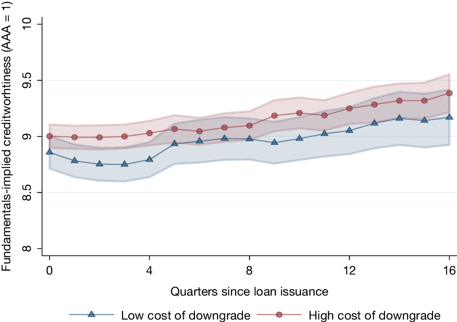
Figure 4 plots the progression of the measure of creditworthiness over the 4-year period following loan issuance for firms with high (above median) and low (below median) cost of downgrade.Footnote 22 The figure shows overall a slight deterioration of creditworthiness during the lifetime of the loan that affects both groups of firms. In addition, there are no distinguishable differences in the progression of the measure between high- and low-cost downgrade firms. In fact, the average difference in the measure of creditworthiness across both groups of firms is only 0.18 notches.
Figure 4 shows the measure of creditworthiness for firms with loans with high (i.e., above median) and low (i.e., below median) costs of downgrade at origination. To construct the measure of creditworthiness, observed (numeric) credit ratings are regressed on firm variables, including leverage, size, profitability, cash flow, and asset tangibility, as well as industry and year fixed effects. Numeric credit ratings reflect the number of notches away from AAA (rating = 1), with a rating of 9 corresponding to BBB and a rating of 8 corresponding to BBB+. The measure of creditworthiness comes from obtaining the fitted values from the regression model. The average cost of a downgrade for the high-cost group (circles) is 22.3 bp, whereas the average cost of a downgrade for the low-cost group (triangles) is 6.7 bp. The analysis is restricted to the first 4 years of each loan’s life. The shaded areas denote the 95% confidence interval for each estimation.

FIGURE 4 Long description
The x-axis is labeled Quarters since loan issuance, ranging from 0 to 16 in increments of 4. The y-axis is labeled Fundamentals-implied creditworthiness (A A A = 1), ranging from 8 to 10 in increments of 0.5.
Two data series are plotted with shaded 95% confidence intervals:
* High cost of downgrade: Represented by a red line with circular markers. It begins at a numeric rating of 9.0 at quarter 0, remains relatively flat until quarter 4, and then trends upward steadily to approximately 9.4 by quarter 16.
* Low cost of downgrade: Represented by a blue line with triangular markers. It starts lower at approximately 8.85 at quarter 0, dips slightly until quarter 3, then follows a similar upward trajectory as the high-cost group, ending at approximately 9.2 at quarter 16.
The high-cost group consistently maintains a higher numeric rating (indicating lower creditworthiness) than the low-cost group throughout the 16-quarter period. The shaded confidence intervals for both groups overlap significantly between quarters 4 and 16.
Next, we provide two additional tests to further mitigate selection concerns. First, we exploit the fact that managers are more likely to possess insider information that is relevant for the short run than for the long run (e.g., Larcker, Levy, Quinn, Tayan, and Taylor (Reference Larcker, Levy, Quinn, Tayan and Taylor2021)).Footnote 23 Specifically, in Table 6, we repeat our main analysis while dropping observations 1, 2, 4, and 8 quarters after loan origination. If managers select into steeper pricing grids because of positive insider information, the relationship between cost of downgrade and probability of downgrade should concentrate in the quarters shortly after loan origination and therefore excluding the early quarters from the sample should weaken the effects shown in Table 3. Inconsistent with this concern, Table 6 shows that the relationship between cost of downgrade and probability of downgrade remains essentially the same irrespective of the time window that we investigate.

TABLE 6 Long description
A data table with four columns labeled 1 through 4, representing time windows excluding the 1st Quarter, 1st Halfyear, 1st Year, and 2nd Years respectively.
Row 1: Cost of downgrade coefficients.
- Column 1: minus 0.635 with three asterisks (standard error 0.204).
- Column 2: minus 0.586 with three asterisks (standard error 0.222).
- Column 3: minus 0.726 with three asterisks (standard error 0.251).
- Column 4: minus 0.590 with two asterisks (standard error 0.283).
Rows 2 through 6: Fixed Effects and Controls.
- Firm F E, Year dash quarter F E, Rating F E, Loan controls, and Firm controls are all marked as Yes for all four columns.
Row 7: Number of observations.
- Column 1: 20,657.
- Column 2: 18,759.
- Column 3: 15,275.
- Column 4: 9,856.
Row 8: R-squared values.
- Column 1: 0.13.
- Column 2: 0.12.
- Column 3: 0.12.
- Column 4: 0.11.
Row 9: Mean of dependent variable.
- Column 1: 2.24.
- Column 2: 2.04.
- Column 3: 2.00.
- Column 4: 1.79.
Second, we follow the corporate governance literature and exploit measures of CEO optimism based on options holdings. Specifically, we proxy for CEO optimism using i) the fraction of CEOs that hold 67% deep-in-the-money options (Campbell, Gallmeyer, Johnson, Rutherford, and Stanley (Reference Campbell, Gallmeyer, Johnson, Rutherford and Stanley2011)) and ii) the fraction of CEOs that hold in-the-money options with less than one year to expiration (Malmendier and Tate (Reference Malmendier and Tate2008)). We add interactions between these measures of CEO optimism and cost of downgrade to our main specification and report the estimation results in Table IA.11 in the Supplementary Material. If CEOs with positive information regarding their firm prospects select into steeper pricing grids, one would expect that the majority of the effect of cost of downgrade is driven by optimistic CEOs (i.e., the coefficients on the interaction terms should be negative and the coefficient on the standalone cost of downgrade should lose its predictive power). However, this is not what Table IA.11 in the Supplementary Material shows. Overall, the results in this section are inconsistent with the proposition that our previous results are driven by self-selection of executives with positive inside information into steeper pricing grids.
Finally, one implication of the previous results is that credit rating inflation should cause ratings to become less accurate over time. That is, a wedge should eventually occur between objective credit quality and nominal credit ratings, similar to the effect caused by credit rating inflation in the RMBS market (Griffin, Nickerson, and Tang (Reference Griffin, Nickerson and Tang2013)). We examine this possibility in Table IA.12 in the Supplementary Material. For each firm in our sample, we proxy for credit quality using Merton’s distance-to-default and then estimate regressions of distance to default on the cost of downgrade. A higher cost of downgrade is associated with a lower distance to default, though this relationship is statistically significant only in the specification with industry-year fixed effects and not in the baseline regression. This approach is appropriate, as default risk is typically highly correlated within industries at any given time, owing to common economic shocks and similar cost and revenue structures among peers. Within each credit rating notch, the pattern in the more stringent specification is generally consistent with the idea that conflicts of interest distort the incentives of CRAs to accurately rate firms.
2. Undisclosed Firm Information
A second potential challenge to our interpretation of the results is that the results could be driven by firms hiding negative financial information from the CRAs rather than by CRAs catering to their clients. CRAs issue credit ratings based on information provided by a borrower, and they do not verify this information (see Section C of the Supplementary Material). Firms whose borrowing costs would experience the highest interest rate increase in the eventuality of a credit rating downgrade have the strongest incentive to hide detrimental information, which could explain why CRAs are less likely to downgrade firms when the downgrade is potentially more costly.
To address this concern, we exploit an observable negative shock to the creditworthiness of a subset of the firms in our sample. Specifically, between the third quarter of 2014 and the end of 2015, commodities experienced a dramatic loss in value, with the Dow Jones Commodity Index plummeting by 50%. Arguably, this loss negatively affected firms that depended on commodity values to generate profits, such as firms from the oil, gas, and mining sectors. Consistent with this proposition, there was significant public concern about the prospects of these affected firms during this time.Footnote 24 The idea of this test is to compare the CRAs’ behavior when they rate firms that were affected by the commodity shock (which the public saw as deteriorated) with the CRAs’ behavior when rating the remaining, unaffected firms. Since the shock was visible and highly public, the ability of borrowers in the affected sectors to hide adverse information was particularly low. If our results are driven by unobserved (i.e., hidden) firm information, we should see a weaker link between the cost of a downgrade and the likelihood of a downgrade among borrowers in the affected sectors during this downturn.Footnote 25
In Table 7, we supplement our main specification with an indicator variable for firms in industry sectors that depend on commodity values (
$ 1(commodities) $
 ), an indicator variable that captures the time when commodity values fell (
$ 1\left( commodities\hskip0.35em shock\right) $
 ), and the interaction of these indicators with
$ cost\hskip0.35em of\hskip0.35em downgrade $
 .Footnote 26 The coefficient on the standalone
$ cost\hskip0.35em of downgrade $
 remains statistically significant and similar in magnitude to the estimates in Table 3 in all specifications. Consistent with falling commodity values adversely affecting borrowers, the coefficient on
$ 1(commodities)\times 1\left( commodities\hskip0.35em shock\right) $
 is positive, ranging from 0.7 to 6.2 pp. However, the coefficient on the triple interaction ranges from
$ - $
 5.7 to
$ - $
 3.9 pp (always statistically significant at the 1% level), indicating that downgrades were concentrated among borrowers for whom the cost of a downgrade is lower. Since arguably all market participants were well aware of these commodity setbacks, these results are inconsistent with the idea that our main results are driven by firms hiding negative financial information. In contrast, these results are consistent with conflicts of interest.

TABLE 7 Long description
The table presents regression results for the dependent variable 1(Downgrade) across four columns labeled 1 through 4.
Key variables and coefficients (standard errors in parentheses):
* Cost of downgrade: -0.629*** (0.238) in model 1; -0.640*** (0.217) in model 2; -0.540** (0.211) in model 3; -0.626*** (0.215) in model 4.
* 1(commodities) times 1(commodities shock): 6.279*** (1.186) in model 1; 3.994*** (1.023) in model 2; 1.121 (1.318) in model 3; 0.841 (1.293) in model 4.
* Cost of downgrade times 1(commodities) times 1(commodities shock): -5.774*** (1.442) in model 1; -4.476*** (1.375) in model 2; -4.048*** (1.492) in model 3; -4.024*** (1.498) in model 4.
* Cost of downgrade times 1(commodities shock): -0.453 (0.620) in model 1; -0.111 (0.576) in model 2; -0.044 (0.552) in model 3; 0.018 (0.553) in model 4.
Fixed Effects (F E) and Controls:
* Firm F E: Yes for all models.
* Year-quarter F E: Yes for all models.
* Rating F E: No for model 1; Yes for models 2, 3, and 4.
* Loan controls: No for models 1 and 3; Yes for models 2 and 4.
* Firm controls: No for models 1 and 2; Yes for models 3 and 4.
* Other interactions: Yes for all models.
Summary Statistics:
* Number of observations: 22,760 for all models.
* R-squared: 0.09 for model 1; 0.11 for model 2; 0.12 for model 3; 0.13 for model 4.
* Mean of dependent variable: 2.57 for all models.
We further examine the possibility that the hiding of negative financial information drives our results in the Supplementary Material. First, we conduct a test based on earnings surprises. Following a similar idea to that of our previous test, we use negative earnings surprises as an unanticipated shock to firm information and quality. Results are presented in Table IA.15 in the Supplementary Material. Similar to the results in Table 7, Table IA.15 in the Supplementary Material shows that in times of negative earnings surprises, the negative relationship between cost of downgrade and probability of downgrade is strongly amplified.
Second, we exploit cross-sectional differences in the ease with which firms can hide or manipulate financial information. Specifically, the idea of this test is to compare i) the CRAs’ behavior when rating firms that are relatively more opaque in nature (i.e., firms that have more room to manipulate their financials) to ii) the CRAs’ behavior when rating the remaining, less opaque firms.
We use a firm’s intangibles divided by total assets and a firm’s R&D expenses as proxies for a firm’s “opaqueness” (Cañibano, Garcia-Ayuso, and Sanchez (Reference Cañibano, Garcia-Ayuso and Sanchez2000), Wyatt (Reference Wyatt2005)). In columns 1 and 2 of Table IA.16 in the Supplementary Material, we supplement our main specification with indicator variables for above-median values of these proxy variables, as well as with the interaction between these indicators and
$ cost\hskip0.35em of downgrade $
 . The coefficients on both interaction terms are statistically insignificant, inconsistent with the proposition that our main results are driven by firms hiding negative financial information from the CRAs.
3. Avoidance of Noninvestment Grade Classification
A third potential challenge to our interpretation of the results is that they could be driven by CRAs being less likely to downgrade a client if the credit rating downgrade would change their client’s classification from investment grade to noninvestment grade. Losing the investment-grade classification could result not only in increased borrowing costs and a lower future availability of funding for borrowers but also reduced investment opportunities for investors. CRAs’ guidelines are clear: Credit ratings should be issued independently of the effect that they may have on the borrower (see Section C of the Supplementary Material). However, when a firm is on the border of a noninvestment grade classification, CRAs may have the implicit consent of investors to avoid downgrading (Bruno et al. (Reference Bruno, Cornaggia and Cornaggia2016)).
To investigate this possibility, we introduce the indicator variable
$ 1\left( border junk\right) $
 , which takes the value 1 when the borrower has a credit rating of BBB− (i.e., just above noninvestment grade), and 0 otherwise. As before, we supplement our main specification with this variable as well as with the interaction between this variable and
$ cost\hskip0.35em of downgrade $
 . We report the results in column 3 of Table IA.16 in the Supplementary Material. While the point estimate on
$ cost\hskip0.35em of downgrade $
 is
$ - $
 0.56 pp (similar to Table 3), the point estimate on the interaction term is statistically insignificant. Overall, this result indicates that CRAs are hesitant to downgrade their clients when the costs of doing so are higher across the whole spectrum of ratings, not just close to the noninvestment grade classification.Footnote 27
4. Prevention of Credit Rating Downgrades by Adjusting Firm Policies
A fourth potential challenge to our interpretation of the results is that they could be driven by firms adjusting their leverage to avoid a credit rating downgrade (e.g., Kisgen (Reference Kisgen2006)). However, inconsistent with this concern, results in the Supplementary Material show that a firm’s cost of downgrade is unrelated to its i) loan and bond issuance activity (Table IA.17 in the Supplementary Material) and ii) investment activity (Table IA.18 in the Supplementary Material). We note that these tests do not imply that firms never manage their credit ratings by adjusting their leverage. Rather, these tests imply that, conditional on having the same initial credit rating, differences in costs of downgrade and probability of downgrade are unrelated to firm leverage policies.
5. Internalization of Externalities
The final challenge to our interpretation of the results is that they could be driven by CRAs internalizing negative externalities to the firms they downgrade. Specifically, a credit rating downgrade can reduce a firm’s access to credit, which subsequently may undermine the firm’s financial health, thereby leading to a self-fulfilling prophecy of creditworthiness deterioration and downgrades (Manso et al. (Reference Manso, Strulovici and Tchistyi2010)). While CRA guidelines explicitly forbid considering the effects of rating actions when issuing or changing ratings (see Section C.4 of the Supplementary Material for excerpts from CRA guidelines), the possibility remains that CRAs differentially deviate more from their guidelines when rating firms with a higher cost of downgrade. While the negative externalities of downgrades should be most prevalent for firms that are close to losing their investment grade classification and thus the fact that our results hold for borrowers irrespective of their initial credit rating mitigates the aforementioned concern (see column 3 of Table IA.16 in the Supplementary Material), we implement two additional empirical tests.
First, we exploit the fact that the internalization of externalities concern should be absent for credit rating upgrades, since these only have positive externalities for borrowers. To test this idea, we first construct a sample of loans with upgrade grids, that is, loans where borrower credit rating at origination is toward the lower end of the grid.Footnote 28 We define two variables: i)
$ 1(upgrade) $
 , which takes the value 1 if the borrower experiences a credit rating upgrade by a CRA in a given quarter, and ii) benefit of upgrade, which measures the lowering in interest rate spreads following a one-notch increase in a credit rating. We then regress
$ 1(upgrade) $
 on the benefit of an upgrade and report the estimation results in Table 8. Column 1 uses the full sample, while column 2 restricts the sample to loans with upgrade grids.

TABLE 8 Long description
The table consists of two columns labeled 1 and 2 under the primary header 1 open parenthesis Upgrade close parenthesis.
Row 1: Benefit of upgrade times 1 open parenthesis upgrade grid close parenthesis. Column 1 is 0.763 with a standard error of 0.996. Column 2 is empty.
Row 2: Benefit of upgrade. Column 1 is minus 0.484 with three asterisks and a standard error of 0.165. Column 2 is 2.107 with one asterisk and a standard error of 1.234.
Row 3: 1 open parenthesis upgrade grid close parenthesis. Column 1 is 2.651 with three asterisks and a standard error of 0.988. Column 2 is empty.
Row 4: Firm F E. Both columns are Yes.
Row 5: Year minus quarter F E. Both columns are Yes.
Row 6: Rating F E. Both columns are Yes.
Row 7: Loan controls. Both columns are Yes.
Row 8: Firm controls. Both columns are Yes.
Row 9: Number of observations. Column 1 is 22,702. Column 2 is 1,889.
Row 10: R-squared. Column 1 is 0.05. Column 2 is 0.15.
Row 11: Mean of dependent variable. Column 1 is 1.70. Column 2 is 3.71.
We find that loans with upgrade grids are more likely to receive upgrades, though the effect is statistically insignificant in the full sample and significant at the 10% level in the subsample. When we include loan fixed effects (Table IA.19 in the Supplementary Material), the effect in the full sample becomes significant at the 5% level.Footnote 29
Next, building on the previous test, we estimate an ordered logit regression, which allows us to incorporate both the cost of downgrades and the benefit of upgrades using a continuous variable. The dependent variable is the change in credit rating, defined such that positive values indicate downgrades and negative values indicate upgrades. Table 9 presents the results. Column 1 reports OLS estimates for completeness and as a benchmark, while column 2 reports the ordered logit results.Footnote 30 Consistent with our earlier findings, the coefficients on the cost of downgrade are negative in both specifications.

TABLE 9 Long description
The table consists of three columns. The first column lists variables and controls, while the second and third columns represent results for O L S 1 and Ordered Logit 2 respectively under the header Worsening in Rating.
* Cost of downgrade: O L S 1 shows minus 0.013 with two asterisks (standard error 0.006). Ordered Logit 2 shows minus 0.141 with two asterisks (standard error 0.066).
* Firm F E: Yes for O L S 1, No for Ordered Logit 2.
* Industry F E: No for O L S 1, Yes for Ordered Logit 2.
* Year-quarter F E: Yes for both models.
* Rating F E: Yes for both models.
* Loan controls: Yes for both models.
* Firm controls: Yes for both models.
* Number of observations: 22,760 for both models.
* R-squared: 0.11 for O L S 1, not applicable for Ordered Logit 2.
* Mean of dependent variable: 0.02 for both models.
Overall, these results are not only inconsistent with the idea that CRAs systematically internalize negative borrower externalities but also suggest that any conflicts of interest may be, to some extent, symmetric.
Second, if CRAs were to internalize the externalities of their downgrade decisions, CRAs should be especially hesitant to issue downgrades when uncertainty is high, for fear of causing unnecessary spillover damages to firms. Thus, if our results are driven by CRAs being more conservative when rating firms with a higher cost of downgrade, then these firms should experience fewer credit rating reversals after a downgrade. To test this conjecture, we introduce the indicator
$ 1(reversal) $
 , which takes the value 1 if a firm receives a credit rating that offsets a previous credit rating change during the lifetime of the same loan (i.e., there was a previous credit rating downgrade followed by a credit rating upgrade or vice versa), and 0 otherwise. We then estimate regressions of
$ 1(reversal) $
 on
$ cost\hskip0.35em of downgrade $
 and report the estimation results in Table IA.21 in the Supplementary Material. We find no relationship between cost of downgrade and the reversal of credit rating decisions.
E. Additional Proxy for Conflicts of Interest
In this section, we consider that, since loans are often rolled over at maturity, a credit rating downgrade shortly before the maturity date can be particularly costly for the borrower, as it negatively affects the terms of a new loan. Accordingly, one would expect loans closer to maturity to be less likely to be downgraded. This relationship also provides a useful benchmark for interpreting the cost-of-downgrade results.
In Table 10, we regress the downgrade indicator on a continuous time-to-maturity variable (column 1) and its interaction with the cost of downgrade (column 2). The results show that loans closer to maturity are less likely to be downgraded, consistent with the idea discussed above, and this effect remains robust after controlling for the cost of downgrade. In economic terms, each additional quarter of remaining maturity is associated with an increase in the probability of downgrade of 9.8–10.9 basis points.

TABLE 10 Long description
The table presents regression results for the dependent variable 1 open parenthesis Downgrade close parenthesis across two columns labeled 1 and 2.
Row 1: Time to maturity open parenthesis quarters close parenthesis shows a coefficient of 0.098 with three asterisks in column 1 and 0.109 with three asterisks in column 2. Standard errors are 0.024 for both.
Row 2: Cost of downgrade multiplied by time to maturity is only present in column 2 with a coefficient of minus 0.061 with two asterisks and a standard error of 0.027.
Row 3: Cost of downgrade is only present in column 2 with a coefficient of minus 0.418 with one asterisk and a standard error of 0.244.
The following rows indicate fixed effects and controls, all marked as Yes for both columns: Firm F E, Year minus quarter F E, Rating F E, Loan controls, and Firm controls.
The bottom section provides summary statistics:
Number of observations is 22,756 for both columns.
R squared is 0.12 for column 1 and 0.13 for column 2.
Mean of dependent variable is 2.57 for both columns.
The previous results provide an alternative perspective on the effect of the cost of downgrade: as shown in Section IV.A, a one standard deviation increase in borrowing costs in the event of a one-notch downgrade reduces the quarterly probability of downgrade by nearly 0.8 pp, equivalent to shortening loan maturity by approximately 7.4 quarters. Overall, these findings support the conclusion that CRAs face significant conflicts of interest, which meaningfully affect their rating behavior.
V. Loan Pricing and the Cost of Downgrades
If CRAs are less likely (or slower) to downgrade a borrower when the costs of doing so are higher for the borrower, loan pricing grids are less effective at compensating the lenders (i.e., investors) for a deterioration in the borrower’s financial health. This may affect loan pricing at the time of loan origination if primary market participants are aware of this problem. Loan contracts that are more affected by the conflicts of interest of CRAs by way of steeper pricing grids should be priced at a discount compared to similar loans with fewer potential agency issues. On the other hand, secondary market participants such as collateralized loan obligation investors or pension funds are arguably less informed than banks in regard to these loan contracts. In this section, we test if agency conflicts stemming from performance sensitive debt are priced in the primary and secondary markets.
A. Loan Pricing and the Cost of Downgrades in the Primary Market
We investigate the relationship between loan spreads and pricing grid design at origination. We introduce the variable
$ average\hskip0.35em cost\hskip0.35em of downgrade $
 , computed as the average cost of downgrade across all rating levels in the initial grid. Thus, this variable is a measure of the ex ante (i.e., expected) conflicts of interest of CRAs captured by the average steepness of the pricing grid, as opposed to a measure of the ex post (i.e., realized) conflicts of interest of CRAs over the life of the loan.Footnote 31 Table 11 shows the results of regressions in which the dependent variable is the loan’s interest rate spread at origination and the independent variable of interest is
$ average\hskip0.35em cost\hskip0.35em of downgrade $
 . As in previous analyses, the variable is standardized, and standard errors are clustered by firm. We retain only one observation per loan (i.e., at origination). Importantly, while the four specifications in Table 11 vary in terms of control variables and fixed effects, they all include firm fixed effects. Thus, the estimations effectively compare loan contracts with different pricing grids by the same borrower.

TABLE 11 Long description
The table presents regression results for Loan Spread across four columns labeled 1 through 4.
* Row 1: Avg. cost of downgrade. Column 1 is 4.683 with three asterisks. Column 2 is 3.823 with three asterisks. Column 3 is 4.106 with three asterisks. Column 4 is 3.685 with three asterisks.
* Row 2: Standard errors for Avg. cost of downgrade. Column 1 is 0.576. Column 2 is 0.438. Column 3 is 0.512. Column 4 is 0.425.
* Row 3: Firm F E. All columns are marked Yes.
* Row 4: Year-quarter F E. All columns are marked Yes.
* Row 5: Rating at origination F E. Column 1 is No. Columns 2, 3, and 4 are Yes.
* Row 6: Loan controls. Column 1 is No. Column 2 is Yes. Column 3 is No. Column 4 is Yes.
* Row 7: Firm controls. Column 1 is No. Column 2 is No. Column 3 is Yes. Column 4 is Yes.
* Row 8: No. of obs. Column 1 is 1,702. Column 2 is 1,697. Column 3 is 1,701. Column 4 is 1,697.
* Row 9: R-squared. Column 1 is 0.77. Column 2 is 0.82. Column 3 is 0.81. Column 4 is 0.83.
* Row 10: Mean of dependent variable. Column 1 is 115.94. Columns 2, 3, and 4 are 116.00.
The point estimates on
$ average\hskip0.35em cost\hskip0.35em of downgrade $
 are positive and statistically significant at the 1% level in the four specifications, ranging from 3.7 to 4.7 bp. Thus, the regression results are consistent with borrowers and lenders being aware of and pricing the conflicts of interest of CRAs.
The previous result can seem somewhat surprising at first, since it indicates that, all else being equal, a steeper pricing grid is detrimental to the borrower (i.e., borrowing costs are higher at origination). Since interest rates increase when the borrower is downgraded, PSD loans effectively embed an insurance mechanism for the lender against the deterioration of the borrower’s financial health. If the pricing grid is steeper, the insurance payment is higher. Intuitively, a loan with a larger premium should be cheaper for the borrower, not more expensive. However, the previous result can be understood in the context of our analysis. Our analysis compares only loans that have a pricing grid to begin with. Specifically, our regressions compare loan spreads across loans that have pricing grids of varying steepness, and the coefficient estimates reflect the decreasing relative efficiency of pricing grids. Compared to a very small increase in interest rates for downgrades, a large increase in interest rates after downgrades is less efficient, since, as the results in Section IV indicate, CRAs are more reluctant to downgrade their clients when the costs of a downgrade are higher.
B. Loan Pricing and the Cost of Downgrades in the Secondary Market
The trading of loans in the secondary market has increased substantially in recent years (Beyhaghi and Ehsani (Reference Beyhaghi and Ehsani2017)).Footnote 32 One concern with these trades is that originating banks may have an advantage over investors in the secondary market because they have superior information regarding loan quality (Dahiya, Puri, and Saunders (Reference Dahiya, Puri and Saunders2003)). While some investors are well-informed and even have access to insider information (Addoum and Murfin (Reference Addoum and Murfin2020)), many, such as mutual funds and loan funds, are nonbank investors (who tend to be less informed). Previously, we showed that the potential for credit inflation is, to some extent, priced at origination. We now investigate whether this pricing of the potential for credit inflation persists once loans are traded in the secondary market.
We obtain secondary market loan pricing data from Refinitiv’s Loan Pricing Corporation (LPC). The secondary market data consist of self-reported information from brokers that quote daily prices on loans. While a quote does not guarantee a trade, brokers tend to make markets for more liquid loans, and any loan in the LPC database is almost surely traded at some point.Footnote 33 We match these data to our sample of PSD loans using a proprietary linking table provided by Refinitiv. The Refinitiv linking table matches 4.1% of the loans in our sample (i.e., 75 loans) to the secondary market data. While this matching rate may seem low, it is similar to the 4.9% matching rate that we find for all loans in DealScan and to the matching rate reported by other research using similar data.Footnote 34 Section A of the Supplementary Material details the matching procedure. Although the sample is small, it supports useful—albeit mostly descriptive—analyses, which are still valuable given the limited evidence on whether secondary market participants price conflicts of interest.
We construct a quarterly panel with quoted prices for the traded loans in our sample and compare the prices of PSD loans with high (i.e., above-median) downgrade cost at origination to the prices of PSD loans with low (i.e., below-median) downgrade cost at origination. Specifically, we estimate a regression where the dependent variable is loan price (measured as the average of the mid-prices quoted each quarter) and the independent variables of interest are the interactions of an indicator for above-median cost of downgrade and indicators for each quarter since loan issuance. The regression includes the same set of control variables and fixed effects as in column 4 of Table 3 (i.e., our most stringent specification) plus loan fixed effects, and we consider the first 4 years of each loan’s lifetime.Footnote 35
Figure 5 shows the coefficients for each quarterly interaction along with their corresponding 95% confidence interval based on standard errors clustered by loan. We use the first quarter’s estimate as our coefficient of reference. The price difference in this quarter is 1.3 pp, meaning the zero line in this graph represents low cost of downgrade loans priced 1.3% higher than high cost of downgrade loans. Thus, since each interaction coefficient captures the average difference in price between PSD loans with high cost of downgrade and PSD loans with low cost of downgrade, a positive coefficient in a given quarter means that the differences in prices between the two groups of loans increased in that quarter relative to the difference that prevailed in the first quarter. Note that an increase in price is equivalent to a decrease in yield. Thus, a positive coefficient implies a decrease in the initial yield premium associated with loans that have a high cost of downgrade.
Figure 5 shows the dynamics of the pricing of loans with high cost of downgrade in the secondary market. Loan price (measured as the average of the mid-prices quoted each quarter) is regressed on the interactions of an indicator for above-median cost of downgrade and indicators for each quarter since loan issuance. The regression includes the same set of control variables and fixed effects as in column 4 of Table 3 plus loan fixed effects, and the first 4 years of each loan’s lifetime are considered. The coefficients associated with the interactions are denoted by solid circles, and the vertical bars denote the corresponding 95% confidence interval (based on standard errors clustered by loan). The dashed vertical line denotes the average time from origination to first sale for loans with above-median cost of downgrade.

FIGURE 5 Long description
A line graph where the Y axis is labeled Effect of high cost of downgrade (% of initial price) with a scale from minus 2 to 8. The X axis is labeled Quarters since issued with a scale from 2 to 16. A horizontal red baseline is set at 0. A vertical dashed line is positioned between quarters 3 and 4.
Data points are represented by solid blue circles with vertical 95% confidence interval bars.
* At quarter 2, the point is slightly below 0.
* At quarter 3, the point is just above 0.
* From quarter 4 to quarter 10, there is a steady linear increase from approximately 0.5 to 1.5.
* At quarter 11, there is a noticeable jump to approximately 2.
* From quarters 12 to 16, the points continue a general upward trend, reaching nearly 4 by quarter 16.
* The vertical confidence interval bars widen significantly as time progresses, particularly from quarter 11 onward, indicating increased variance in the later quarters.
The figure shows that there is no change in price differences between high and low cost of downgrade loans in the first three quarters after loan origination. Coincidently, the average time from origination to first recorded sale for loans with above-median cost of downgrade is 100 days (denoted by the dashed vertical line in the figure). From the fourth quarter onward, coefficient estimates turn positive, consistent with a decrease in the premium associated with high cost of downgrade loans as they are sold to secondary market participants. On average, these loans become about 2% more expensive than low cost of downgrade loans 3 years after the first quarter of trading. Overall, the point estimates in Figure 5 are consistent with secondary market participants overpaying for above-median cost of downgrade loans (and therefore pricing less of the conflicts of interest of CRAs) relative to originating banks.
C. Probability of Trade and Time to First Trade
To complement the previous analysis, we also study whether there is a relationship between a loan’s cost of downgrade, its probability of being traded, and the speed at which it is first traded. We continue to focus on the 75 loans in our sample for which we have secondary market pricing data. Since this sample is relatively small and the nature of this analysis is cross-sectional, we lack the additional observations provided by the quarterly-panel structure from the previous section. Consequently, we display the results graphically.
We begin by investigating whether banks are more likely to sell loans with higher CRA conflicts. To facilitate the comparison between loans that are traded and loans that are not traded, we match the 75 loans with similar nontraded loans using a nearest neighbor matching technique based on all continuous control variables.Footnote 36 We then split these 150 observations into three groups based on their cost of downgrade and plot the probability of a loan being sold by the originating bank for each group in Figure 6.
Figure 6 shows the probability of loan trade in the secondary market by terciles of average cost of downgrade. The sample consists of 75 traded loans and 75 nontraded loans. The nontraded loans are selected so that they resemble the traded loans using a nearest neighbor matching framework based on firm characteristics (current credit rating, size, profitability, asset tangibility, and leverage) and loan characteristics (amount, number of financial covenants, loan type, and whether the loan is secured or not).

The figure shows a nonlinear relationship between our measure of CRA conflicts and the likelihood of a loan being traded. Loans in the highest group of cost of downgrade have a 58% probability of being traded in the secondary market, almost 10% higher than that of the other two groups with lower downgrade costs.
Next, we investigate whether banks, conditionally on selling a loan, are selling loans with higher CRA conflicts faster. The underlying assumption for this analysis is that originating banks sell parts of the loan on the same day a dealer quotes a price for the loan for the first time. Thus, we compare the time elapsed between loan origination and when the loan gets quoted for the first time across groups of loans based on costs of downgrade. As before, we split the sample into three groups based on cost of downgrade and plot the average time-to-first-trade for each group in Figure 7.
Figure 7 shows the average time-to-first-trade (days) in the secondary market by terciles of average cost of downgrade. The sample consists of 75 traded loans.

Once again, the figure shows a nonlinear relationship between our measure of CRA conflicts and the outcome variable. Loans in the lowest group of cost of downgrade stay on banks’ balance sheets for about 470 days before getting quoted, whereas loans in the other two groups experience their first quote after about 200 days, on average. This is a 270-day difference, equivalent to a 57% relative change. Overall, the results in this section are consistent with banks being more likely to sell loans with a higher potential for credit rating inflation. The results are also consistent with these loans being traded faster. Note that we only observe quotes for the most liquid loans that have brokers providing daily prices. Since 40% (i.e., about 8 times as many loans as in our sample) are traded (Beyhaghi and Ehsani (Reference Beyhaghi and Ehsani2017)), the actual number of loans and investors affected by CRA conflicts is arguably quite large.
VI. Credit Rating Agency Behavior and Settlements with the DOJ
Recently, both S&P and Moody’s agreed to settlements with the DOJ for failing to adhere to their standards when rating securitized products during the run-up to the financial crisis.Footnote 37 The statements of facts indicate that both CRAs deviated from their methodologies without disclosing those changes to investors or the public. Moreover, both CRAs avoided the downgrading of underperforming assets because doing so could negatively affect their business (see Section C of the Supplementary Material for excerpts from these statements of facts). The results in Section IV show that the conflicts of interest of CRAs were pervasive and were not restricted to structured products. S&P and Moody’s also avoided downgrading their clients when the downgrade would translate into an increase in the borrowing costs associated with their PSD obligations. Consistent with CRAs catering to their clients, this reluctance to downgrade is driven precisely by those instances in which the CRA’s credit rating is the decisive one in determining borrowing costs.
As a result of these settlements, CRAs committed to improving their credit models, becoming more transparent, and addressing conflicts of interest more generally. In this section, we investigate whether CRAs have delivered on these commitments.
The question of whether CRAs improved their approach to credit ratings post-settlements cannot be answered by studying the securitized products market, where the infractions linked to the settlements occurred. The main limitation is that the nonagency RMBS and CDO markets virtually disappeared after the financial crisis. In contrast, in our setting of PSD loans, issuances have remained relatively stable during the last 15 years (Figure IA.1 in the Supplementary Material).
We study whether the relationship between the probability of a downgrade and the increase in borrowing costs after a downgrade varies with the settlements. We introduce the indicator variable
$ 1\left( post- settlement\right) $
 , which takes the value 1 from the second quarter of 2015 (i.e., the quarter after S&P settled with the DOJ) and 0 before the second quarter of 2015. We focus on the date of S&P’s settlement because i) our data coverage ends in December 2016 (i.e., before the Moody’s settlement) and ii) the first (and largest) settlement in the history of CRAs is likely to affect the rest of the market. Once again, we supplement our main specification with this variable, as well as with the interaction between this variable and the cost of a downgrade.
The estimation results are presented in Table 12. All specifications include the complete set of controls and fixed effects. If CRAs changed their approach to credit ratings to deal with conflicts of interest post-settlement, the coefficient on the interaction term should be positive. However, column 1 of Table 12 shows a statistically insignificant and negative coefficient on
$ cost\hskip0.35em of downgrade\times 1\left( post- settlement\right) $
 .Footnote 38 In contrast, consistent with the results in Section IV, the coefficient on the standalone variable that represents the cost of a downgrade continues to be statistically significant and negative. Column 2 of Table 12 also yields a statistically insignificant coefficient on
$ cost\hskip0.35em of downgrade\times 1\left( post- settlement\right) $
 when considering the time required for the firm to be downgraded after loan origination as the dependent variable in the regression.

TABLE 12 Long description
A table with three columns. The first column lists variables, the second column is labeled 1 (Downgrade) Model 1, and the third column is labeled Time to Downgrade Model 2.
* Cost of downgrade: -0.513 with three asterisks (standard error 0.176) in Model 1; 1.396 with two asterisks (standard error 0.560) in Model 2.
* Cost of downgrade multiplied by 1 (post-settlement): -0.587 (standard error 0.476) in Model 1; 1.223 (standard error 2.523) in Model 2.
* Firm F E: Yes for both models.
* Year F E: No for Model 1; Yes for Model 2.
* Year-quarter F E: Yes for Model 1; No for Model 2.
* Rating F E: Yes for both models.
* Loan controls: Yes for both models.
* Firm controls: Yes for both models.
* Number of observations: 22,760.00 for Model 1; 247.00 for Model 2.
* R-squared: 0.11 for Model 1; 0.74 for Model 2.
* Mean of dependent variable: 1.57 for Model 1; 6.10 for Model 2.
In the Supplementary Material, we consider the possibility that immediately after the financial crisis, CRAs may have changed their credit rating behavior due to the potential threat of litigation. In Table IA.25 in the Supplementary Material, we estimate regressions similar to those in Table 12, replacing the post-settlement indicator with a postcrisis indicator, which takes a value of one from 2008 to 2015. The interaction coefficient between the cost of downgrade and the postcrisis indicator is statistically indistinguishable from zero in both the downgrade (column 1) and time-to-downgrade (column 2) regressions, indicating no evidence of a change in behavior. As a refinement, Figure IA.2 in the Supplementary Material shows the effect of the cost-of-downgrade variable on the probability of a downgrade year by year throughout the sample period, confirming that the results are consistent across all years.
Overall, the previous results suggest that the DOJ settlements did not have the intended effect of improving credit rating quality, and CRAs did not change their credit rating behavior, at least almost 2 years after the settlement and when rating firms associated with PSD. Notably, these results are also consistent with recent allegations by the Securities and Exchange Commission that credit rating catering has resurfaced after the recovery of the RMBS market (see https://www.sec.gov/news/press-release/2022-205).
VII. Conclusion
We show evidence that conflicts of interest affect the behavior of CRAs, specifically in the context of credit rating-dependent PSD. CRAs are significantly less likely to downgrade borrowers if these downgrades would translate into larger increases in borrowing costs for their clients. This behavior is driven by instances in which the CRA’s credit rating is the decisive one in determining loan spreads and by instances in which the CRA rates clients that are potentially more profitable for the agency. This indicates that CRAs cater to their clients outside the market for complex structured products. Even conditionally on eventually downgrading, CRAs delay their decision when the costs of downgrading are higher.
The potential for credit inflation is, to some extent, priced at origination. This suggests that borrowers and lenders are aware of these problems. In contrast, secondary market participants do not seem to internalize the conflicts of interest of CRAs: yield premiums decrease when these loans are sold. In addition, also consistent with originating banks internalizing the additional risk, originating banks are more likely to sell loans with high costs of downgrade, and among the loans that they sell, loans with high cost of downgrade are also sold faster. A concerning implication of these findings is that originating banks, arguably the most informed market participants and the ones in an ideal position to monitor CRAs, have little incentive to do so.
Overall, our results suggest that the catering behavior of CRAs is not confined to complex markets such as the securitized products market. The major CRAs settled with the DOJ for inflating the credit ratings of nonagency RMBSs and CDOs during the run-up to the financial crisis, and they renewed their commitment to credit rating quality. However, we find no evidence of reduced catering in the market for PSD post-settlements. This result calls into question the effectiveness of the settlements in influencing CRA behavior, and it highlights the pervasiveness of these conflicts of interest that stem from the issuer–pays business model of CRAs.
Appendix Variable Description
Borrower-Quarter Characteristics
- Assets:
-
Total assets (in billions USD)
- Credit rating:
-
Long-term issuer credit rating. Either from S&P or Moody’s depending on which CRA is decisive. Ratings are converted into a numerical scale ranging from 1 (AAA/Aaa) to 22 (D), following the standard ordering of S&P and Moody’s long-term rating categories (e.g., 1 = AAA/Aaa, 2 = AA+/Aa1, 3 = AA/Aa2, …, 10 = BBB–/Baa3, …, 22 = D).
- Leverage:
-
Total liabilities $ \div Assets $

- Loan volume:
-
Cumulative volume of loans issued in the rolling 4-year windows prior to each loan, excluding the actual loan
- Profitability:
-
EBITDA $ \div Assets $
- 1(border junk):
-
Indicator variable that takes the value of 1 if the borrower has a credit rating of BBB-, and 0 otherwise
- 1(commodities):
-
Indicator variable that takes the value of 1 if the firm is in the oil and gas extraction, coal mining, metal ore mining, or the support activities for mining sectors (i.e., NAICS codes 2111, 2121, 2122, and 2131), and 0 otherwise.
- Intangibles over assets:
-
Intangibles $ \div Assets $
- 1(high intangibles):
-
Indicator variable that takes the value of 1 if intangibles divided by assets is above the sample median, and 0 otherwise.
- R&D:
-
Research and development expenses (in millions USD)
- 1(high R&D):
-
Indicator variable that takes the value of 1 if R&D is above the sample median, and 0 otherwise.
- 1(high-yield issuer):
-
Indicator variable that takes the value of 1 if the borrower has a credit rating at of BB+ or lower, and 0 otherwise.


Loan Characteristics at Origination
- All in spread drawn:
-
All in spread drawn above LIBOR
- Loan size:
-
Total loan size (in millions USD)
- Loan type:
-
Set of indicator variables for the following loan types: i) revolver, ii) term loan, and iii) other. The “other” category primarily includes facilities such as acquisition facilities, bridge loans, and standby letters of credit.
Loan-Quarter Characteristics
- Cost of downgrade:
-
The increase in a loan’s interest spread that results from a credit downgrade of one notch (in basis points).
- Cost of 2-notch downgrade:
-
The increase in a loan’s interest spread that results from a downgrade of two notches (in basis points).
- Cost of downgrade (% of assets):
-
The increase in the costs that results from a downgrade of one notch measured as $ Cost\hskip0.35em of downgrade\times Loan\hskip0.35em size\div Assets $
. - 1(decisive rating):
-
Indicator variable that takes the value of 1 if the CRA holds the decisive rating, and 0 otherwise.
- 1(commodities shock):
-
Indicator variable that takes the value of 1 from 2014:Q3 to 2015:Q4, and 0 otherwise.
- 1(post settlement):
-
Indicator variable that takes the value of 1 from 2015:Q2 to 2016:Q4, and 0 otherwise.

Supplementary Material
To view supplementary material for this article, please visit http://doi.org/10.1017/S0022109025102391.