A New Look at the Old Terms of Trade Debate

Debate over trends in the terms of trade between primary products and manufactures, their causes and their impact, has dominated the growth and development literature for almost two centuries. Classical economists claimed that the relative price of primary products should improve over time, since land and other natural resources were in inelastic supply while capital and labour were not. The experience over the half-century or so before the 1870s proved them right: the relative price of manufactures underwent a spectacular decline, while those of primary products soared (see Figures 1 and 2). In the early 1950s, however, Raúl Prebisch and Hans Singer challenged the classical view, asserting that the terms of trade of the primary-producing third world had deteriorated since the late nineteenth century.Footnote ¹ Prebisch, indeed, calculated that in the 1930s a given quantity of primary products would purchase only 63 per cent of the finished manufactures that could have been bought in the 1860s.Footnote ²

Fig. 1.

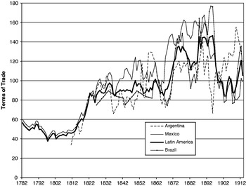
The Poor Periphery: Net Barter Terms of Trade, 1796–1913 (1900=100). Source: Williamson, ‘Globalization and the Great Divergence: Terms of Trade Booms and Volatility in the Poor Periphery 1782–1913’, European Review of Economic History, vol. 12, no. 3 (2008), p. 365.

Fig. 2.

Latin America: Net Barter Terms of Trade, 1782–1913 (1900=100).

Source: Williamson, ‘Globalization and the Great Divergence: Terms of Trade Booms’, p. 366.

Prebisch and Singer argued that this secular deterioration in the terms of trade damaged growth potential in the periphery. Yet they never really tested their hypothesis, and since theory tells us that a deterioration in the terms of trade, equivalent to a relative rise in the price of manufactures, must also have stimulated industry in the poor periphery, the Prebisch–Singer hypothesis may be in doubt.Footnote ³ The pre-1870s secular upswing of the terms of trade in the periphery clearly caused primary-product export-led growth, and deindustrialisation.Footnote ⁴ However, Prebisch, Singer and their followers ignored a symmetric corollary: on the downside following the 1870s, deterioration in the secular terms of trade implied a stimulus to import-competing industry in the periphery.Footnote ⁵ Prebisch and Singer stressed instead the short-run economic damage that a relative fall in commodity prices would do to a periphery specialising in primary products. The literature generated by Prebisch and Singer has another weakness. Typically, it deals with the relative price of primary products in world markets as a whole, not with the terms of trade facing any given primary-product-exporting country. Prebisch, Singer and the literature that followed never assessed the economic impact on the poor periphery of the secular fall, or of a cessation of the rise, in its terms of trade. Rather, they assumed it.

We try to do better when assessing the Latin American industrialisation experience after 1870, those critical decades before the economic disaster of the interwar years, and before the introduction of anti-global import substitution industrialisation (ISI) policies between the 1930s and 1970s. In addition, we try to assess the relative contribution of world prices and domestic policy towards the performance of the Latin American industrial leaders. The next section uses new evidence to establish the timing and location of Latin American industrialisation, with a primary focus on Argentina, Brazil, Chile and Mexico. Industrialisation was fastest in Brazil and Mexico, especially when compared with the rest of Latin America, the Middle East and most of Asia. Why? We then list the leading potential (though not necessarily competing) explanations for this impressive industrialisation performance: changing world prices, changing productivity, changing policy and changing wage competitiveness. We stress changing, because it is change in the rate of industrialisation that we wish to explain. The following sections explore these in turn, starting with the dramatic reversal in trends in the net barter terms of trade in much of Latin America, especially compared with the rest of the periphery. We argue that if, as the conventional literature asserts, a spectacular rise in the net barter terms of trade caused deindustrialisation in the periphery prior to 1870 (through ‘Dutch Disease’ effects), then their stability or fall thereafter must have helped cause what might be called ‘reindustrialisation’. The next section explores the possible role of an acceleration in total factor productivity (TFP) growth in the export sector, especially mining. The latter should have raised the income terms of trade, and, as Edward Beatty has argued so persuasively for Mexico, it should have contributed to export-led industrialisation.Footnote ⁶ We ask whether the Mexican experience was exceptional, or whether it was repeated in other Latin American industrial leaders. We then consider other sources of Latin America's increasing industrial competitiveness in its own markets, such as cheaper food, which might keep the nominal industrial wage low, and then the impact of real exchange rate depreciation, a force that would have improved the competitiveness of local manufacturing against foreign imports. The paper concludes with a tentative judgement about the relative importance of changes in prices, policies and productivity, and suggests a future research agenda for augmenting the Latin American country sample and improving the evidence documenting these potential explanations.

Measuring the Industrial Lift-off Across Latin America

We are not the first to argue that industrialisation started long before the 1930s in Latin America, indeed, even before World War I. There is a vast body of literature supporting this argument.Footnote ⁷ Warren Dean made the case for Brazil, and Luis Ospina Vázquez for Colombia, at a time when dependency theory and the assumption that the late nineteenth century was a period solely of export-led growth were the dominant paradigms.Footnote ⁸ In the 1970s Ezequiel Gallo made a similar case for Argentina, Rosemary Thorp and Geoffrey Bertram for Peru, and Henry Kirsch for Chile.Footnote ⁹ A decade later, Stephen Haber made the case for Mexico.Footnote ¹⁰ While impressive, what is missing from this pioneering literature is an explicit comparative assessment of the timing, pace and location of industrialisation in Latin America, and a comprehensive assessment of its causes. We try to fill part of that gap here.

Whether measured by employment, output or value added, textile production dominated manufacturing in the late nineteenth century, and it is also the best-documented sector of industry, so we start there. Imports satisfied a significant part of Latin American total textile demand in the 1870s. Mexico, for example, imported 40 million square metres of cloth in 1879, compared with 60 million square metres produced domestically.Footnote ¹¹ Thus foreigners supplied 40 per cent of the domestic market. Yet these same data imply that domestic producers were able to claim 60 per cent of the local market, a fairly large amount for a country that had been flooded with cheap, factory-made, European textiles for almost a century. Indeed, Table 1 documents that domestic textile manufactures controlled 75 per cent of the home market in the 1800s, so European imports increased their share from 25 to 40 per cent over the seven decades of deindustrialisation. But things were even worse elsewhere in the poor periphery. The share of the domestic market supplied by India's local textile producers fell from 95 per cent in 1833 to 35–42 per cent in 1877, the latter much lower than Mexico's 60 per cent in 1879.Footnote ¹² The deindustrialisation forces were even more powerful in the Ottoman Empire, where the local textile industry's market share of domestic demand fell from 97 per cent in the early 1820s to only 20–26 per cent in the 1910s.Footnote ¹³ They were equally powerful in Indonesia, where the local textile industry's market share of domestic demand fell from 82 per cent in 1822 to 11 per cent in 1913.Footnote ¹⁴ Thus, despite the significance of foreign imports, the Mexican textile industry had been able to fend off some of the foreign invasion of manufactures up to the 1870s, at least compared with the rest of the periphery.Footnote ¹⁵ Nonetheless, deindustrialisation and Dutch Disease effects were certainly ubiquitous up to the 1870s. But note what happened after the 1870s: the Mexican textile industry was able to win back all it had lost and more so by 1906–8. Powerful reindustrialisation forces were at work in Mexico during the years of the Porfiriato.

Table 1.

Comparative Industrialisation in Latin America, 1800s–1913: Manufacturers' Import Penetration

Sources: Textile Sources: Mexico 1800s and 1879 from Dobado González et al., ‘Mexican Exceptionalism’, Table 4; Mexico 1906–8 from W. A. Gregory Clark, Cotton Goods in Latin America, Part i: Cuba, Mexico, and Central America (Washington DC, Department of Commerce, Special Agents Series no. 31, 1909), pp. 20 and 39; Peru from Thorp and Bertram, Peru 1890–1977, p. 34; Colombia 1870s from José Antonio Ocampo, ‘El sector externo de la economía colombiana en el siglo XIX’ (paper presented at the Seminario Internacional sobre Historia Económica de Colombia en el Siglo XIX, Banco de la República, Bogotá, 15–16 Aug. 2007), p. 35; Brazil 1907 from W. A. Gregory Clark, Cotton Goods in Latin America, Part ii: Brazil, Colombia, and Venezuela (Washington DC, Department of Commerce, Special Agents Series no. 36, 1910), p. 6; Argentina 1913 reports two estimates, the lower from L. S. Garry, Textile Markets in Argentina, Uruguay and Paraguay (Washington DC, Department of Commerce, Special Agents Series no. 194, 1920), pp. 22 and 31, and the upper from Adolfo Dorfman, Historia de la industria argentina (Buenos Aires, 1970), p. 310.

Other Sources: Mexico 1903–11 from Compañía Fundidora de Fierro y Acero de Monterrey, Annual Report to the General Assembly (Mexico City, 1923); Argentina from Dorfman, Historia de la industria argentina, p. 310.

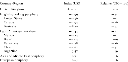
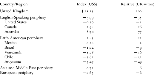
Table 2 offers another index of industrial performance at the end of the period, net exports (+) or imports (−) of cotton textile manufactures per capita in 1910, an index that includes yarn, thread and cloth of all sorts. While, once again, it is limited to (cotton) textiles, it augments the Latin American observations to include five countries – Argentina, Brazil, Chile, Mexico and Venezuela – and offers comparisons with other parts of the periphery. The United Kingdom, the world leader, had a net cotton textile export position of US$ 11.25 per capita. The remainder of the regions listed in Table 2 recorded a net import position (−), but note that Mexico had a net import balance close to zero (US$ 0.24 per capita), a figure lower than the United States (US$ 0.36)! No Latin American country did better than Mexico, the closest competitor being Brazil (net imports of US$ 1.04 per capita), and most did far worse. Indeed, Argentina (net imports of US$ 5.47) joined Australia (US$ 8.70) in recording the highest dependence on imported cotton textile manufactures in the periphery.

Table 2.

An Index of Industrialisation in Latin America around 1910: Net Exports (+) and Net Imports (−) Per Capita of Cotton Manufactures

Sources: Trade data are from US Department of Commerce, Bureau of Foreign and Domestic Commerce, The Foreign Commerce and Navigation of the United States (Washington DC, 1912), Tables 106 and 107, pp. 214–19. Population data are from A. Maddison, Monitoring the World Economy 1820–1992 (Paris, 1995).

Note: Regional averages are unweighted.

We have already discussed the nineteenth-century evidence in the first panel of Table 1, where estimates of the share of the home market for textiles supplied by domestic industry are reported. Now consider the early twentieth-century evidence. Two notable facts emerge. First, by the early part of the century, Brazil's domestic textile industry had carved out an impressive share of its local market, 65.3 per cent in 1907. While this was considerably smaller than that of Mexico, 77.9 per cent, it was far higher than in the Ottoman Empire (20–6 per cent), India (39 per cent), or Dutch Indonesia (11 per cent).Footnote ¹⁶ By this measure alone Brazil and Mexico were more successful industrially than the rest of the periphery. Peru was very successful in developing its textile industry up to the end of the 1890s, but the rate of growth of the industry declined thereafter.Footnote ¹⁷ Argentina, on the other hand, could report very little development of its textile industry by 1913, local firms claiming only 15.5 to 17.5 per cent of the home textile market. Food processing was the most important branch of manufacturing in Argentina, but unfortunately we do not have the data documenting this sector to make a comparison similar to that carried out for textiles. So much for light industry. Theory tells us to expect much less heavy industry in early industrialisation since it takes time to develop a comparative advantage in such skill- and capital-intensive industries. The second panel of Table 1 is consistent with theory: it reports smaller market shares for heavy industrial product groups. Still, what data we do have reports the market shares of domestic heavy industry to have been on a steep rise for Mexico: the country's domestic producers' share of the local iron and steel market rose from 6 to 28 per cent between 1903 and 1911, while that for coke rose from 17 to 47 per cent. The 1913 figure for metals and machinery in Argentina was 12 per cent, about a decade behind Mexico.

This trade evidence offers strong support for the view that the Latin American industrial leaders did indeed experience a lift-off before 1913, and certainly long before the 1930s and its early ISI policies. However, we want to know more about exactly when the lift-off took place before we ask why it took place.

Stephen Haber dates the beginning of the Mexican industrial lift-off to the late 1880s. Almost half a century after Mexico's initial mechanisation efforts, industry in 1888 was, according to Haber, still small and unproductive, although he might have added that it was considerably larger and more productive than almost anywhere else in the poor periphery. But in the decade that followed, ‘the industry more than doubled in size. By 1911, the industry had grown an additional 50 per cent. Estimates of total factor productivity (TFP) growth … indicate increases of between 1.5 per cent (lower bound) and 3.3 per cent (upper bound) per year. Labour productivity grew even faster … between 3.0 and 4.7 per cent per year.’Footnote ¹⁸ Such growth rates meant that Mexican textile producers had displaced most imported cloth by 1914.Footnote ¹⁹ Furthermore, by about 1910, the Mexican textile industry had a machine per worker index 77 per cent that of Britain, suggesting that Mexican technology had been partially catching up over the previous four decades. Furthermore, Mexico was not the only part of Latin America with that distinction: Brazil and Peru recorded machine/worker indices (67 and 78 per cent of that of Britain, respectively) higher than China (34), India (33), Japan (52), Greece (39), Egypt (65), Austria-Hungary (65) and even Germany (63).Footnote ²⁰

Tables 1 and 2 confirm Haber's inference: the first shows that Mexican net imports of cotton manufactures per capita were almost zero in 1910, and the second shows that local producers claimed more than three-quarters of the domestic market for all textiles in 1906–8. The only foreign textiles still being imported were high-quality, fine-weave fabrics. Table 1 also suggests a modification to Haber's dating of the Mexican lift-off; the trade data suggest that it got an even earlier start than 1888.

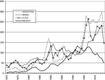
In an effort to better identify the Latin American industrial leaders and the timing of their industrialisation experience in the decades before the First World War, Table 3 and Figure 3 report evidence based on exports to Latin America from the United States and the United Kingdom. These were the main suppliers of industrial intermediates, energy sources and capital goods used in Latin American industry, so we assume that imports of manufacturing machinery, iron and steel, and coal (all in constant US dollars) are good proxies for relative industrial growth. Tables 3 and 4 and Figure 3 allow us to compare industrialisation progress among Latin American countries between 1870 and 1914. Others have used similar data before, but not comparatively as we do here.Footnote ²¹ Xavier Tafunell, Albert Carreras and César Yáñez have used data documenting capital goods exports to Latin America to estimate gross capital formation levels in 20 Latin American countries between 1890 and 1930.Footnote ²² Their work has shown that these data are reliable, and that most machinery exports to Latin America came from just three sources: the United States, the United Kingdom and Germany.Footnote ²³

Fig. 3.

Index of Coal, Iron and Steel, and Machinery Imports in Constant US Dollars, 1870–1914 (1900=100). Source: See Appendix.

Table 3.

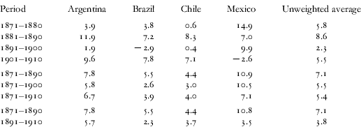
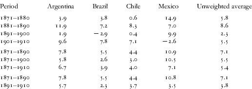
Growth Rates Per Annum in Intermediates and Capital Goods. Imports from the US and UK (US$) 1871–1911 (per cent)

Sources: The imports data are reported exports in 1890–1914 US dollars from the US and the UK in iron and steel, coal and manufacturing machinery. The US data are taken from US Department of Commerce, Bureau of Foreign and Domestic Commerce, The Foreign Commerce and Navigation of the United States (Washington DC), 1870–1913. The UK data are taken from UK, Annual Statement of the Trade of the United Kingdom with Foreign Countries and British Possessions, Parliamentary Papers, 1870–1914.

Table 4.

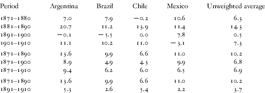
Growth Rates per annum in Manufacturing Capital Goods Imports from the US and UK (US$) 1871–1911 (in %)

Sources: The import data are reported exports of manufacturing machinery in 1890–1914 US dollars from the US and the UK: see Table 3 for details.

Here we consider only the iron and steel products and machinery that were used by manufacturing. Following Wilson Suzigan, we exclude machinery used in mining, construction, agriculture, railways and electricity generation.Footnote ²⁴ The exclusion of items not related to manufacturing is more difficult to achieve with the iron and steel data since most of these imports were used for several purposes. Yet, whenever the category explicitly referred to purposes other than manufacturing, we excluded it.Footnote ²⁵ We aggregate imports from the United States and the United Kingdom only.Footnote ²⁶ Since we wish to compare trends and not the levels of machinery imports across Latin America, it is unlikely that the exclusion of German and other countries' machinery exports to Latin America distorts the picture.Footnote ²⁷

Figure 3 plots the import time series for the combination of manufacturing machinery (hereafter machinery), iron and steel (hereafter iron), and coal from 1870 to 1914 (1900=100). According to this proxy, all four of the Latin American countries plotted there – Argentina, Brazil, Chile, and Mexico – exhibited impressive growth over the four decades. True, three of them experienced high volatility: Argentina, Brazil and Chile all recorded large booms in the late 1880s and early 1890s, and again in the run up to the First World War, as well as a big bust in the 1890s. Mexico did not undergo this volatility before 1900, but it did undergo a secular slowdown from 1902 up to and during the Revolution (1910–20).Footnote ²⁸

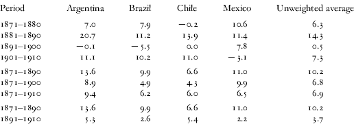
Tables 3 and 4 report the growth rates of both proxies (in US dollars). Table 3 documents growth rates of the combined import package: the volatility of Argentina, Brazil and Chile is revealed once more, and so is Mexico's dominant industrialisation up to 1902. Import growth rates increased in the 1880s relative to the 1870s in all countries; in the 1890s they declined in Brazil, Argentina and Chile, but not in Mexico. However, between 1901 and 1911 Mexico's growth rate became negative while the other three countries recovered their 1881–91 growth rates.Footnote ²⁹ Between 1871 and 1901, Mexico grew almost twice as fast as the average (10.5 versus 5.5 per cent per annum), and it grew a bit slower when the run-up to the Revolution is included (7.1 per cent between 1871 and 1911, versus 5.4 per cent per annum). In addition, Table 3 shows that the lift-off started during the first two decades of this period, not just after 1888 as Haber argues.

The growth of imports of manufacturing machinery reported in Table 4 repeats the findings of Table 3: prior to 1901, Mexican growth rates exceed the average, 9.9 per cent versus 6.8 per cent per annum. However, the growth of Mexican machinery imports for the whole period (1871–1911) was 6.5 per cent, a bit lower than the 6.9 per cent average for the four republics. Its growth rate before 1891 (11 per cent) exceeds those afterwards (2.2 per cent), primarily because of the setbacks that occurred after 1901.

These data are consistent with Henry Kirsch's documentation of slow Chilean industrialisation using other evidence. The slow growth in capital goods imports for the 1870s (Tables 3 and 4) is consistent with the view that industrialisation got under way only after the War of the Pacific (1879–84). Kirsch estimates that, while relatively modest compared with Argentina, Brazil and certainly Mexico, Chilean industrial activity increased from 1880 to 1913 at an average annual rate of growth of 2.1 per cent, but that the 1880–90 and 1900–10 decades experienced a little more robust growth (3 per cent), while the period between 1890 and 1900 appears to have been one of stagnation. Table 3, Table 4 and Figure 3 document patterns of decadal growth similar to those described by Kirsch.Footnote ³⁰ In short, the Chilean performance was much more modest than that of the other three countries analysed. According to Gabriel Palma this was in part due to the fact that nitrate exporting did not call for local processing activities, nor for large amounts of manufacturing inputs or machinery, and therefore it did not generate backward linkages to local manufacturing.Footnote ³¹ In other words, Dutch Disease effects suppressed Chilean industrialisation.

Wilson Suzigan argues that industrial growth in Brazil started at the end of the 1860s after the war with Paraguay (1865–70).Footnote ³² His position is consistent with the slow growth in capital goods imports that Tables 3 and 4 document for the 1871–81 period. Between 1880 and 1895 Brazil experienced rapid industrial growth, a performance that is consistent with the coffee export boom and rising immigration. However, industrial investment fell during the 1890s with the bust in coffee export markets in 1896–1901. Investment rates recovered in 1902, initiating a new era of expansion until 1913: indeed, the decade before 1913 recorded the fastest growth in Brazil's capital goods imports.

According to Fernando Rocchi, Argentine factories were virtually non-existent until the 1870s. But after the 1873 crisis local manufacturing began to grow. Rocchi's industrial output figures show annual growth averaging 8.1 per cent for the decade following 1880, followed by a decline to 3 per cent in the 1890s, and 4.7 per cent for the decade 1900–10.Footnote ³³ The modest growth rates after 1890 hardly exceed population growth (3.2 per cent per annum), and they are consistent with the abrupt fall in the growth rates of capital goods imports shown in Table 4.Footnote ³⁴ The 1880s boom must have been partly a result of the unprecedented capital inflows that went into Argentina during that decade, when it attracted between 40 and 50 per cent of all British overseas lending, enabling the government to finance large infrastructure projects. After the Baring Crisis in 1890 the interest rate premium rose for Argentina and for other Latin American republics, making foreign capital more expensive, choking off foreign investment, and thus contributing to the slowdown of capital goods imports in Argentina, Brazil and Chile during the 1890s.Footnote ³⁵ Although Rocchi thinks that most Argentine manufacturing firms grew during the 1890s, our capital goods import data suggest that the recovery was slow until 1902, after which it increased at unprecedented rates until the 1907 crisis.Footnote ³⁶ Over the full period between 1871 and 1911, Argentina recorded the highest growth in imports of manufacturing machinery in Latin America, 9.4 per cent compared to a regional average of 6.9 per cent, although that wide margin is diminished when we use per capita figures.

To summarise, this section documents the following points: industrialisation in the leading Latin American economies was very impressive between 1870 and 1913; the industrial lift-off started well before 1890; Mexico recorded the most rapid industrialisation before 1901; and after 1900 Argentina, Chile and Brazil all recorded rapid industrial growth, while Mexico's growth rates declined.

Some Potential Explanations for the Latin American Industrial Lift-off

What explains the timing and location of the Latin American industrial lift-off? While the available evidence may not yet permit definitive answers, we think it is useful to assess the initial plausibility of five leading possibilities.

First, we now know that Latin America was far more protectionist than anywhere else in the late nineteenth century.Footnote ³⁷Figure 4 shows that Latin America had the highest tariffs in the world from the late 1880s onwards (Argentina, Brazil, Chile, Colombia, Peru and Mexico were among the most protectionist countries), and that before the late 1880s only the United States had higher average tariff rates.Footnote ³⁸ Still, the typical average tariff rate in Latin America did not rise by much between 1870 and 1914, and it is changes in protection that matter.

Fig. 4.

Unweighted Average of Regional Tariff Before the Second World War. Source: John H. Coatsworth and Jeffrey G. Williamson, ‘Always Protectionist? Latin American Tariffs from Independence to Great Depression’, Journal of Latin American Studies, vol. 36, part 2 (2004), Figure 2.

Certainly there were substantial differences in tariff policy between the Latin American republics. Figure 5 shows that Colombia had the most steeply rising tariff rates. Argentina, however, did not introduce a more protectionist regime during the four decades. On the contrary, its ad valorem tariff rates declined after 1899. Mexico started from extremely high tariff rates and experienced an important decline in them during the 1890s. In Chile the Congress legislated higher specific duties in 1897 and exempted a wide range of intermediate inputs from tariffs.Footnote ³⁹ However, ad valorem rates declined as a consequence of inflation after 1894.Footnote ⁴⁰Figure 5 shows that ad valorem tariff rates in Brazil underwent no significant upward trend, but recorded great volatility throughout the period.Footnote ⁴¹ This was hardly a policy favourable to Brazilian industrialisation. In short, average levels of protection did not rise much, if at all, over the four decades in Argentina, Brazil, Chile or Mexico. But what about the protection of manufacturing, and what about the effective rate of protection there? Here the story is quite different.

Fig. 5.

Tariff ad valorem rates in major Latin American countries. Sources: Data underlying Coatsworth and Williamson, ‘Always Protectionst?’, Figure 3. For Mexico: 1885–90, Sandra Kuntz Ficker, El comercio exterior de México en la era del capitalismo liberal 1870–1929 (Mexico, 2007), p. 220; 1873, 1874 and 1891–1914 kindly provided by Graciela Márquez.

As the leader of the policy pack, Mexico adopted far more coherent and consistent pro-industrial tariff policies under the Porfirian regime. Policymakers in late nineteenth-century Latin America were certainly aware of infant industry arguments, but tariffs were not used specifically and consciously to foster industry in Mexico until the early 1890s.Footnote ⁴² Mexico sharply increased its average tariff rates in 1890 and graduated from having the lowest levels of protection among major Latin American countries to having levels similar to the rest. But this policy transformation did not just entail a change in tariff levels. It also entailed a profound change in the tariff structure, a change which served to raise the effective rate of protection for manufacturing. Edward Beatty and Graciela Márquez have argued persuasively that the 1880s and 1890s saw the introduction of a modern pro-industrial policy in Mexico, including a rational structure of protection.Footnote ⁴³ This policy was followed with a lag elsewhere in Latin America: Brazil and Chile a little later in the 1890s, and Colombia in the early 1900s.Footnote ⁴⁴ Oddly enough, Argentina did not join this policy trend. As Fernando Rocchi has argued, ‘The kind of protectionism Argentine authorities displayed in the period 1880–1930 was nowhere near being [pro-industrial] but rather was a result of lobbying activities on specific items. Actually [net levels of protection were much lower than those that] Edward Beatty had found in Porfirian Mexico between 1880 and 1910.’Footnote ⁴⁵

Haber agrees with Márquez and Beatty: ‘In 1891 Mexico was using tariffs to protect the cotton textile industry [which perhaps would have otherwise been uncompetitive] … This meant high tariffs on competing goods and low tariffs on inputs. The tariff on imported cloth tended to be twice that of the tariff on imported raw cotton. The result was an effective rate of protection that varied from 39 to 78 per cent.’Footnote ⁴⁶ This explanation is especially appealing since it helps account for the fast industrial lift-off in Brazil and Mexico compared with the rest of the periphery. Most of Asia and the Middle East did not have the autonomy to pursue pro-industrial policies, and we also know that Mexico's pro-industrial policy led the rest of the autonomous Latin American republics by a decade or two. Still, the magnitude of the change in the level of manufacturing protection does not seem large enough to account for more than a small share of the industrial lift-off in any of the Latin American leaders.

Now consider four other influences that might have contributed even more to the industrial lift-off in Latin America. The first is world prices and the net barter terms of trade. As shown below, there was a large secular reversal in world relative price trends facing most Latin American economies after the 1870s, a change that no longer penalised local manufacturing, and textiles in particular. Elsewhere, we have shown that a good part of the exceptionally modest Mexican deindustrialisation experience in the century before 1870 was due to an exceptionally modest terms of trade boom from the 1800s to the 1870s compared with the rest of Latin America, Asia and the Middle East.Footnote ⁴⁷ We believe that the same was true of the half-century after 1870, but in the opposite direction: as shown below, Latin America's net barter terms of trade fell earlier and faster than anywhere else in the periphery, especially in Mexico. Second, there was also an acceleration in TFP growth in one key export activity in Latin America, mining (including the nitrate industry). This served to contribute to the fall in the net barter terms of trade, but, given a price elastic demand facing most metals (and chemicals such as nitrate), it also served to raise the income terms of trade. It appears that these productivity events were unusual for the poor periphery at that time, including much of Latin America itself. Third, there is some evidence supporting the view that, compared with the rest of the periphery, Latin American industry may have been kept more competitive since it faced weaker upward pressure on the nominal wage, forces induced by weaker upward pressure on food prices. The latter could be explained by low policy barriers on food imports and the domestic market integration stimulated by the railways. Finally, there is the impact of the depreciation of local currencies to consider. As we shall see, the biggest real exchange rate depreciation between 1870 and 1913 took place in Brazil and Mexico, forces which must have contributed to their relatively impressive industrialisation performance.

No More Dutch Disease in Latin America?

In the 1870s, Latin America faced a large secular change in world relative price trends, a change that no longer penalised local manufacturing. Furthermore, the secular change was bigger and earlier than elsewhere in the poor periphery. The spectacular Dutch Disease effects that had dominated until the 1870s evaporated thereafter.

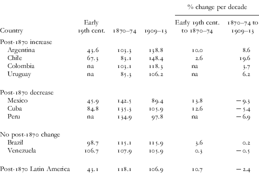
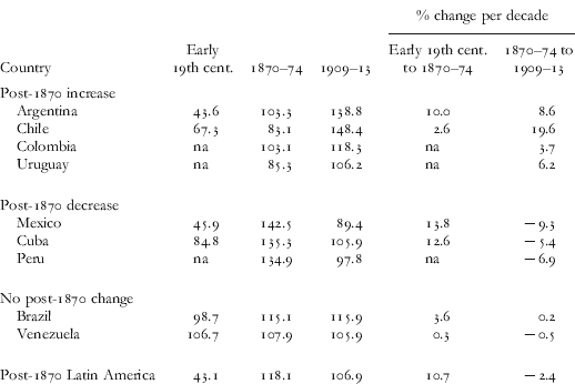
Figure 1 (p. 665, above) shows that the net barter terms of trade for Latin America reached a secular peak in the mid–late 1870s after a seven-decade rise, dropped, then rose again to the early–mid-1890s (regaining the previous peak), after which the index fell far more dramatically up to the early 1900s than elsewhere in the periphery. It never recovered even a third of the previous peaks by 1913. In 1912 net barter terms of trade were only 21 per cent of what they had been in 1895. Between 1870–4 and 1909–13, the terms of trade in Latin America fell by 10 per cent (2.4 per cent per decade, see Table 5), this after rising by 174 per cent, or 10.7 per cent per decade, over the 70 years between 1800–4 and 1870–4.Footnote ⁴⁸ In contrast, the rest of the periphery underwent no net fall over the four decades: the Middle East and Southeast Asia underwent a continuous improvement in terms of trade from the mid-1870s onwards, while South Asia and East Asia experienced no change either way. Figure 2 (p. 666, above) and Table 5 show which parts of Latin America underwent the biggest reversal in the terms of trade trend.

Table 5.

Net Barter Terms of Trade Changes in Latin America: Early Nineteenth Century to 1900–13 (1900=100)

Sources: Williamson, ‘Globalization and the Great Divergence: Terms of Trade Booms’, data underlying Table 2.

Note: Latin America is an 1870 population weighted average. In calculating the percentage change per decade before 1870–4, the country starting points depend on data availability. Thus the starting ponts are Argentina (1810–14), Chile (1810–14), Mexico (1800–4), Cuba (1830–4), Brazil (1826–9) and Venezuela (1830–4).

Only two countries, Argentina and Chile, continued the century-long terms of trade boom until the First World War. As we shall see, Colombia and Uruguay experienced a modest increase, and the rest underwent no change or suffered a fall. Mexico had the biggest fall in its terms of trade after the early–mid-1890s: the index fell by half between 1890 and 1902, a decline twice that of the remainder of Latin America.Footnote ⁴⁹ Furthermore, while the primary products boom in the decade or so before 1913 is reflected in a rise in terms of trade everywhere in the poor periphery, the rise was very modest in Mexico, and it did not come close to recovering the secular peak in the late 1870s and early 1880s. Indeed, the Mexican terms of trade fell by 37.2 per cent (or 9.3 per cent per decade) between 1870–4 and 1910–13 (Table 5). While Mexico was exceptional, there were other Latin American deviants, namely Cuba (−21.7 per cent) and Peru (−27.5 per cent). Brazil and Venezuela experienced hardly any change at all in their terms of trade over the four decades. The important point is that even stability or a modest rise after 1870 represented a marked change in world economic conditions after 70 years of sharply rising terms of trade for Latin America, and thus sharply falling relative prices of manufactures.

Table 5 documents the magnitudes on the upside of the great Latin American terms of trade boom: to repeat, on average the net barter terms of trade rose by 10.7 per cent per decade from the early nineteenth century to the 1870s, and this happened all over Latin America. In some republics the reversal was huge: Mexico underwent a change from +13.8 per cent per decade on the upside to −9.3 per cent on the downside, for an enormous net change of 23.1 percentage points per decade; and Cuba went from +12.6 to −5.4, for another big net change of 18 percentage points per decade. But on average the net change was large for Latin America as a whole: that rise of 10.7 per cent per decade up to the 1870s was followed by a fall of 2.4 per cent per decade afterwards, for a net change of 13.1 percentage points per decade.

In summary, a fall (or no rise) in the net barter terms of trade implied a rise (or no fall) in the relative price of imported manufactures, an event which favoured (or no longer penalised) domestic industry. If, as the literature has long argued, rising terms of trade caused deindustrialisation and Dutch Disease effects in the six or seven decades before the 1870s, it follows that a falling or stable terms of trade index after 1870 should have helped cause a good share of the industrialisation experience among the Latin American leaders up to 1913, even though Argentina and Chile were not among them.Footnote ⁵⁰

Productivity Change, the Income Terms of Trade, and Export-Led Growth

Thus far it has been assumed that the Latin American republics had no influence over their export or import prices, and thus that their terms of trade were determined exogenously in world markets. While this was certainly true of those countries in Table 5 whose commodity exports were only a small share of world exports of that commodity, such as Argentina (maize, wheat), Colombia (coffee, gold), Cuba (sugar, tobacco), Peru (sugar, copper), Uruguay (wool, meat) and Venezuela (coffee, cacao), it certainly was not true of the others in Table 5: Chile (nitrates, copper), Mexico (silver) and Brazil (coffee, rubber). Indeed, Beatty has argued that Mexican mineral supplies to the world market, especially silver, did in fact help to precipitate the large decline in its net barter terms of trade: by flooding the market with silver, Mexico lowered the world price and worsened its terms of trade.Footnote ⁵¹ Beatty also argues that it was rapid productivity advance in Mexican mining that produced that result, but since the demand for minerals was price elastic, total export values and foreign exchange earnings boomed, creating export-led growth.

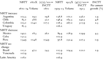
Figure 6 describes the two hypotheses. In case 6B, the country takes its export prices as exogenous: export prices fall in world markets (from P to P′), but domestic supply expands sufficiently fast (S to S′) to offset the price decline, augmenting total export revenue. One can imagine an even greater domestic supply shift (to S″ ) which would have produced more exports and more foreign exchange earnings. Clearly, whatever economic success was observed in this case would be attributed unambiguously to the domestic export supply growth, rather than to changing conditions in world markets. More to the point of this paper, the fall in its net barter terms of trade (P_X/P_M) could not have been a powerful industrialisation stimulus in this case since the improved relative price of industrial output must have been at least partially offset by the improved productivity in the commodity export sector that pushed S outwards.Footnote ⁵² This case seems to apply to Cuba, Peru and Venezuela, countries which experienced a decline in their net barter terms of trade (Table 5) and only a very modest improvement in their income terms of trade (Table 6). Now consider the case in 6B, where export prices rise (from P to P″), a case which appears to apply to Argentina and Colombia, both of which underwent a large increase in their net barter and their income terms of trade. There was no stimulus to industrialisation in this case either, but rather deindustrialisation and Dutch Disease penalties.

Fig. 6.

Alternative Views of the Terms of Trade in Latin America. 6A. The Endogenous Export Price Hypothesis; 6B. The Exogenous Export Price Hypothesis.

Table 6.

Income Terms of Trade (INCTT) Growth 1870–1913 (1900=100)

Sources: The NBTT data are taken from the sources underlying Figure 5, and Latin America is an 1870 population weighted average. The export (X) volume data are taken from Angus Maddison, The World Economy in the 20th Century (Paris, 1989), p. 140, and Angus Maddison, Monitoring the World Economy, 1829–1992 (Paris, 1995), p. 236. INCTT=(NBTT)(X) or XP_X/P_M, where P_X is the export prices and P_M the import prices. The table uses the first equation.

Now consider Beatty's hypothesis in case 6A. Here, the same export supply expansion (S to S′) lowers the country's export price since it is a big player in world markets. But given a price elastic demand, and given an additional outward shift in demand (D to D′), export revenues and foreign exchange earnings expand: the bigger the outward supply shift (and productivity advance in the export sector), the bigger the fall in the net barter terms of trade and the rise in the income terms of trade.Footnote ⁵³ Mexico appears to be the Latin American exception: a very large decline in the net barter terms of trade, after a long secular boom, was consistent with a very large increase in the income terms of trade. While Table 6 confirms Beatty's prediction, his supply-side argument cannot apply to minerals-producing Chile, since its net barter terms of trade did not fall, but rather rose. Table 6 also suggests that Beatty's hypothesis gets ambiguous support at best for Brazil, where its post-1870 net barter terms of trade trend was flat (with great short-run volatility) and its income terms of trade underwent only a modest increase.

Industrial Competitiveness in Latin America: Keeping the Lid on Wages?

The share of the 1895 Latin American labour force in manufacturing never exceeded 25 per cent.Footnote ⁵⁴ Employment shares like these imply that real wages – nominal wages divided by the cost of living (w/P_C) – were determined by labour productivity elsewhere in the economy, in mining, construction, agriculture and services, rather than in manufacturing. Slow-growing labour productivity in the rest of the economy would have given Latin American manufacturing the advantage of modest upward pressure on per unit wage costs, making it more competitive with North America and western Europe, where the upward pressure was much stronger. It was, of course, the own-wage that mattered to employers in manufacturing, that is, the nominal wage divided by the price of manufactures (w/P_M). Since the price of foodstuffs (P_A) was a large component of the cost of living, a fall in P_A/P_M would have improved wage competitiveness in Latin American manufacturing compared with foreign firms. Is there any reason to think that P_A/P_M should have fallen? Yes, and in two respects: first, to the extent that the post-1870s grain invasion flooded Latin America in the food deficit regions; and second, to the extent that railways brought cheaper grain to urban markets in the interior where much Latin American manufacturing was located.Footnote ⁵⁵ The issue is, how much?

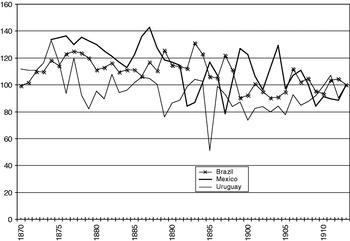
Figure 7 reports P_A/P_M trends for three countries which offer the necessary times series data: Brazil, Mexico and Uruguay. Mexico recorded the biggest P_A/P_M decline from 1874–8 to 1913, 34 per cent; Brazil the second, 21 per cent; and Uruguay the third, 11 per cent. Thus, the grain-invasion-cum-railways prediction is confirmed, and, furthermore, the two fastest industrialising countries recorded the biggest fall in P_A/P_M.

Fig. 7.

Prices of Food Relative to Manufactures (1913=100). Source: See Appendix.

But did cheaper grains necessarily mean lower nominal wages and thus greater wage competitiveness of local manufacturing? Figure 8 reports the own-wage facing manufacturing firms (w/P_M) for four countries which offer the necessary time series data: Brazil, Chile, Mexico and Uruguay. Based on this evidence it appears that Brazil and Uruguay had the industrial advantage on this score, since the upward pressure on the own-wage in manufacturing was much greater in Chile and Mexico. Indeed, over the period 1870–1913 as a whole, the own-wage in Brazil grew no faster than it did in the United States, the former remaining competitive with the latter on that score at least. By the same criteria, wage competitiveness in Chile deteriorated relative to the United States, as it did in Mexico (but not as much as Chile). Of course, there were other forces determining competitiveness, but if we are looking for explanations for precocious industrialisation in Chile and Mexico, better wage competitiveness was not one of them. Nor does it appear likely to have played a big role in Brazil.

Fig. 8.

Own-Wage in Latin American Manufacturing (1913=100). Source: See Appendix.

Did Real Currency Depreciation Increase Manufacturing Profitability?

Depreciation of the domestic currency favours local manufacturing since it makes imported manufactures more expensive in the local market. Currency appreciation does the opposite. When trading partners have different rates of inflation, the nominal exchange rate must be adjusted to take account of the differential inflation rates, yielding a real exchange rate. The real exchange rate (RER) is yet another force that could have helped account for the timing and location of industrialisation in Latin America before 1913.

In a previous working paper we reported RER trends for four Latin American republics: Argentina, Brazil, Chile and Mexico.Footnote ⁵⁶ The evidence clearly showed that manufacturing in Chile must have been greatly disadvantaged by real exchange rate trends, since it underwent significant real currency appreciation. This was even more true of Colombia, which experienced a 20 per cent real currency appreciation between 1881 and 1899, followed by an even more spectacular appreciation during the inflation of the period between 1899 and 1905.Footnote ⁵⁷ The appreciation of the RER must have suppressed the first symptoms of modern industrial development in Colombia during the late nineteenth century, delaying that process until the early twentieth century.Footnote ⁵⁸ Argentina underwent no secular change in its real exchange rate between 1884 and 1913, so it could not have been a source of any stimulus to import-competing manufacturing there. However, the real exchange rate did undergo secular depreciation in Brazil and Mexico, and the magnitudes appear to have been large. Mexico experienced a real currency depreciation of 137 per cent between the mid-1870s and 1902, when capital goods imports surged, and the real currency depreciation for the whole period was an enormous 81 per cent. Brazil also underwent a significant, though not quite so large, real currency depreciation of 34 per cent between 1870–4 and 1913.

In short, some part of the industrial lift-off in Brazil and Mexico can indeed be explained by a real exchange rate depreciation up to 1913. This was not true of Argentina, Chile or Colombia.

A Future Research Agenda: Decomposing the Sources of the Industrial Lift-off

This paper does not offer any explicit empirical decomposition of the sources of the industrial lift-off in Latin America between 1870 and the First World War, although we certainly hope that future research will do so. At this point, we do not believe the evidence is yet sufficient for that demanding task. We have thus been content to lay out five possible explanations, to offer what we hope is some plausible support for them, and to set out an agenda to strengthen the case.

Our strong expectation is that changing fundamentals, in the form of institutions and government, will end up playing a less dominant role in contributing to the industrial lift-off than the current development literature supposes.Footnote ⁵⁹ We stress the word changing, since it had to have been changing fundamentals raising productivity in manufacturing, or changing external terms of trade, or changing domestic wage competitiveness, or changing tariffs, or changing real exchange rates, improving profitability in manufacturing. It would have been those changes that accounted for the lift-off, not the levels of any of these contending forces.

This paper has paid little attention to rising total factor productivity in Latin American manufacturing. There are two explanations for its omission. First, manufacturing productivity growth has not yet been systematically estimated for Latin America for the four decades after 1870, except for Mexico, or for other poor periphery regions with which Latin America might be compared. The debate desperately needs this information. Second, we know that the United States, Britain and other competitors to Latin American manufacturing were themselves undergoing rapid productivity advance, so we would have to find evidence of even faster TFP growth in the Latin American leaders in order to explain industrial growth there. While the data are not yet available to offer much more than an informed guess, ours is that such evidence will be hard to find. Until our guess is confirmed, we are left with this key question: if it was not productivity catch-up in Latin American manufacturing that explains the industrial lift-off, what was it?

Changing external terms of trade must have played a significant role, as the immense pre-1870 boom in the external terms of trade gave way to a post-1870 rise (or at least no fall) in the relative price of imported manufactures. What had been a virulent Dutch Disease before 1870 became a healthy ‘Dutch revival’ after 1870. Furthermore, the two industrial leaders – Mexico, followed by Brazil – experienced the biggest reversals in their secular terms of trade trends. Thus, relative price trends favoured industrialisation in these two republics compared to much of the rest of the poor periphery. These terms of trade forces were strong, and it is time for the literature to pay more attention to them. Yet they did not prevail in Argentina and Chile, which implies that this took the steam out of any industrial stimulus in those two republics.

Changing tariff and real exchange rate policy also must have played a large role, at least in some parts of Latin America. Average tariff rates in Latin America rose hardly at all over these four decades, but the effective rate of protection for manufacturing rose a lot as the tariff structure was rationalised. Since Mexico led the way, it had the ‘first strike’ advantage of effective pro-industrial policy, and this was long before the early ISI protectionist policies of the 1930s. In addition, the real exchange rate for both Brazil and Mexico depreciated, offering more benefits to import-competing industry. Since the other major Latin American republics, including Argentina, did not experience the same real currency depreciation, the two leaders enjoyed a pro-industrial advantage, long before the well-known real currency depreciations of the 1930s. In addition, we now have two reasons why industrialisation in Argentina and Chile should have lagged behind that in Brazil and Mexico: terms of trade trends and commercial policies were both far less favourable to manufacturing.

We doubt that improved wage competitiveness played a role, since the effects, though positive, seem to have been too small to matter much.

This paper has documented impressive industrialisation rates in the Latin American leaders, Brazil and Mexico, between 1870 and 1913. The next step is to seek more precise answers to the ‘sources of industrialisation’ question regarding the quantitative roles of changing prices, policy and productivity. The answers for the pre-1913 period should give us a much better understanding of the twentieth-century Latin American experience with industrialisation, especially when it is compared with the ISI policy epoch between the 1930s and 1970s, as well as with the free trade epoch that followed.