

1 Introduction
Taylor–Couette (TC) flow of a viscous fluid in the annular gap between two concentric cylinders, where one or both cylinders are rotating, is a classical turbulent flow that exhibits interesting shear-flow phenomena (Taylor Reference Taylor1923; Coles Reference Coles1965; Grossmann, Lohse & Sun Reference Grossmann, Lohse and Sun2016). TC flow is perhaps more experimentally accessible than the related plane-Couette (PC) flow (e.g. Pirozzoli, Bernardini & Orlandi Reference Pirozzoli, Bernardini and Orlandi2014) owing to the cylindrical geometry and the convenience of torque measurement. The parameter space covered by most experimental and computational studies of TC flow includes independent Reynolds numbers associated with inner and/or outer cylinder, rotational speed and cylinder radius ratio. There is also a distinction between co-rotating and counter-rotating cylinder motion. TC flow can be defined by two independent length and two independent velocity scales. For incompressible TC flow of a Newtonian fluid, this gives four dimensionless numbers, which typically are the radius ratio  $\unicode[STIX]{x1D702}=R_{i}/R_{o}$, the inner and outer Reynolds numbers
 $Re_{i}=\unicode[STIX]{x1D6FA}_{i}R_{i}d/\unicode[STIX]{x1D708}$ and
 $Re_{o}=\unicode[STIX]{x1D6FA}_{o}R_{o}d/\unicode[STIX]{x1D708}$, respectively, and the ratio of cylinder angular velocities
 $a=-\unicode[STIX]{x1D6FA}_{o}/\unicode[STIX]{x1D6FA}_{i}$. Here
 $\unicode[STIX]{x1D6FA}_{i}$,
 $\unicode[STIX]{x1D6FA}_{o}$ are the rotation angular velocities of the inner and outer cylinders, respectively,
 $R_{i}$,
 $R_{o}$ are the radii of the inner and outer cylinders,
 $\unicode[STIX]{x1D708}$ the kinematic viscosity of the fluid and
 $d=R_{o}-R_{i}$ is the radial gap. Additionally, a fifth number
 $\unicode[STIX]{x1D6E4}=L_{y}/d$, for evaluating the effect of a spanwise domain, can be important, where
 $L_{y}$ is the spanwise domain size. Alternative specifications are sometimes useful, such as the Taylor number
 $Ta$, the Nusselt number
 $Nu$ for the purpose of analogy with Rayleigh–Bénard flow and
 $Re_{w}$, a Reynolds number based on the standard deviation of the radial velocity Huisman et al. (Reference Huisman, van Gils, Grossmann, Sun and Lohse2012).
Figure 1 of Andereck, Liu & Swinney (Reference Andereck, Liu and Swinney1986), reproduced as figure 2 of Grossmann et al. (Reference Grossmann, Lohse and Sun2016), shows a classification of observed flow types in an  $Re_{i}-Re_{o}$ plane up to moderate Reynolds number
 $Re_{i}\approx 2000$. These include wavy vortex flow, modulated waves, spiral turbulence and Taylor vortex flow among others. The review article of Grossmann et al. (Reference Grossmann, Lohse and Sun2016) surveys and summarizes research on these fluid-dynamical phenomena associated with TC flow. At sufficiently large
 $Re_{i}$ (or Taylor number
 $Ta$, which for
 $Re_{o}=0$ is proportional to
 $Re_{i}^{2}$) they argue that the near-wall layers on the cylinder walls become turbulent, signalling a transition toward what is referred to as an ‘ultimate regime’ defined in terms of the large Reynolds number scaling of the Nusselt number with the Taylor number. Here, the two cylinder wall layers appear to conform to the classical law of the wall and are separated by a region of bulk flow that is dominated by large-scale phenomena such as spanwise Taylor roll structures that, at sufficiently large Reynolds numbers, may themselves be turbulent (Lathrop, Fineberg & Swinney Reference Lathrop, Fineberg and Swinney1992a,Reference Lathrop, Fineberg and Swinneyb; Huisman et al. Reference Huisman, van Gils, Grossmann, Sun and Lohse2012). A mechanism for the locking of the turbulent Taylor vortex is discussed by Sacco, Verzicco & Ostilla-Mónico (Reference Sacco, Verzicco and Ostilla-Mónico2019).
Experiments at different  $\unicode[STIX]{x1D702}$ have been conducted in this regime in the range
 $Ta=10^{11}{-}10^{13}$ (Van Gils et al. Reference Van Gils, Huisman, Bruggert, Sun and Lohse2011, Reference Van Gils, Huisman, Grossmann, Sun and Lohse2012; Merbold, Brauckmann & Egbers Reference Merbold, Brauckmann and Egbers2013). These show a Nusselt number
 $Nu$ – the ratio of torque required to maintain the motion to the laminar-flow torque – variation with
 $Ta$ that can be reasonably approximated over this range by
 $Nu\sim Ta^{p}$ where
 $p$ is less than
 $0.5$.
Ostilla-Mónico et al. (Reference Ostilla-Mónico, Verzicco, Grossmann and Lohse2016) report direct numerical simulation (DNS) of TC flow with the outer cylinder stationary up to  $Re_{i}=3\times 10^{5}$ for
 $\unicode[STIX]{x1D702}=0.909$. This corresponds to a maximum Taylor number
 $Ta=9.969\times 10^{10}$. Their DNS shows two Taylor rolls and also demonstrates that the bulk region separating the cylinder wall layers consists of a region of almost constant mean angular momentum density with magnitude equal to the average of that corresponding to the rotational motion of the two cylinders.
Presently, Taylor–Couette flow at relatively large Reynolds numbers is investigated using the numerical technique of large-eddy simulation (LES). Our aim in part is to provide data at larger  $Re_{i}$ than is presently available from DNS as a prelude to wall-modelled LES at even larger
 $Re_{i}$. Parameter values
 $\unicode[STIX]{x1D702}=0.909$ with
 $Re_{o}=0$ and
 $Re_{i}=10^{5},3\times 10^{5},6\times 10^{5},10^{6}$ are used, with a maximum Taylor number
 $Ta=1.108\times 10^{12}$. In § 2 we outline the numerical method and the subgrid-scale model for our wall-resolved LES. This is followed in § 3 by an account of the present LES results. Good agreement with the DNS of Ostilla-Mónico et al. (Reference Ostilla-Mónico, Verzicco, Grossmann and Lohse2016) is obtained at our lower
 $Re_{i}$. The higher
 $Re_{i}$ results show a clear log-like profile for the wall layer of the inner cylinder. All LES reproduce a bulk inner region with almost constant azimuthal–spanwise-averaged angular momentum. Section 4 describes an empirical, one-dimensional (radial) model for the mean TC flow for relatively large Reynolds numbers and cylinder co-rotation. This comprises wall-bounded regions with law-of-the wall mean-velocity profiles together with a uniform angular momentum central region. The model is closed with a scaling hypothesis concerning the relative thickness of the inner wall layer. It is shown that the model gives satisfactory agreement with experiment, DNS and LES for several important mean-flow parameters. In § 5 an extension of the model to rough-wall layers is described, while concluding remarks are presented in § 6.
2 Large-eddy simulation
2.1 LES equations
The governing equations for LES of incompressible viscous flow are derived by formally applying a spatial filter to the Navier–Stokes equations to give
 $$\begin{eqnarray}\frac{\unicode[STIX]{x2202}\tilde{u} _{i}}{\unicode[STIX]{x2202}t}+\frac{\unicode[STIX]{x2202}\tilde{u} _{i}\tilde{u} _{j}}{\unicode[STIX]{x2202}x_{j}}=-\frac{\unicode[STIX]{x2202}\tilde{p}}{\unicode[STIX]{x2202}x_{j}}+\unicode[STIX]{x1D708}\frac{\unicode[STIX]{x2202}^{2}\tilde{u} _{i}}{\unicode[STIX]{x2202}x_{j}^{2}}-\frac{\unicode[STIX]{x2202}T_{ij}}{\unicode[STIX]{x2202}x_{j}},\quad \frac{\unicode[STIX]{x2202}\tilde{u} _{i}}{\unicode[STIX]{x2202}x_{i}}=0,\end{eqnarray}$$
with  $\tilde{u} _{i}$ the filtered velocity and
 $\tilde{p}$ the filtered pressure (divided by density), and where
 $T_{ij}=\widetilde{u_{i}u_{j}}-\widetilde{u_{i}}\widetilde{u_{j}}$ denotes the effect of subgrid scales on the resolved-scale motion. In practice, this is represented on a computational grid using a subgrid-scale (SGS) model. Cylindrical coordinates (
 $r,\unicode[STIX]{x1D703},y$) with velocity components (
 $u_{r},u_{\unicode[STIX]{x1D703}},u_{y}$) are convenient for diagnosing results. General curvilinear coordinates
 $(\unicode[STIX]{x1D702},\unicode[STIX]{x1D709},y)$ will be described for the implementation of the numerical method.
2.2 Numerical method
In the curvilinear coordinate system, the (formally) filtered governing equations in conservation-law form can be written as (Zang, Street & Koseff Reference Zang, Street and Koseff1994)
 $$\begin{eqnarray}\frac{\unicode[STIX]{x2202}U^{m}}{\unicode[STIX]{x2202}\unicode[STIX]{x1D709}^{m}}=0,\quad \frac{J^{-1}\unicode[STIX]{x2202}\tilde{u_{i}}}{\unicode[STIX]{x2202}t}+\frac{\unicode[STIX]{x2202}F_{i}^{m}}{\unicode[STIX]{x2202}\unicode[STIX]{x1D709}^{m}}=0,\end{eqnarray}$$
where  $U^{m}$ and
 $F_{i}^{m}$ are given as
 $$\begin{eqnarray}U^{m}=J^{-1}\frac{\unicode[STIX]{x2202}\unicode[STIX]{x1D709}^{m}}{\unicode[STIX]{x2202}x_{i}}\widetilde{u_{i}}\quad \text{and}\quad F_{i}^{m}=U^{m}\widetilde{u_{i}}+J^{-1}\frac{\unicode[STIX]{x2202}\unicode[STIX]{x1D709}^{m}}{\unicode[STIX]{x2202}x_{j}}T_{ij}+J^{-1}\frac{\unicode[STIX]{x2202}\unicode[STIX]{x1D709}^{m}}{\unicode[STIX]{x2202}x_{i}}\tilde{p}-\unicode[STIX]{x1D708}G^{mn}\frac{\unicode[STIX]{x2202}\widetilde{u_{i}}}{\unicode[STIX]{x2202}\unicode[STIX]{x1D709}^{n}},\end{eqnarray}$$
respectively, where  $J^{-1}$ is the inverse of the Jacobian and
 $G^{mn}$ is the mesh skewness tensor defined as:
 $$\begin{eqnarray}J^{-1}=\det \left(\frac{\unicode[STIX]{x2202}x_{i}}{\unicode[STIX]{x2202}\unicode[STIX]{x1D709}^{j}}\right),\quad G^{mn}=J^{-1}\frac{\unicode[STIX]{x2202}\unicode[STIX]{x1D709}^{m}}{\unicode[STIX]{x2202}x_{j}}\frac{\unicode[STIX]{x2202}\unicode[STIX]{x1D709}^{n}}{\unicode[STIX]{x2202}x_{j}}.\end{eqnarray}$$
A semi-implicit fractional step method was used to solve the governing equations with successive solution of the modified Helmholtz equations that result from implicit treatment of the viscous terms, pressure Poisson equation and the velocity correction step. Integration in time is implemented using an Adams–Bashforth method for explicit terms and Crank–Nicolson for implicit terms. A parallel multi-grid solver with a line-relaxed Gauss–Seidel iteration method is used for numerical solution of the Poisson equation. The spatial discretization of the nonlinear term utilizes a fourth-order, non-staggered, energy-conservative scheme of the skew–symmetric form (Morinishi et al. Reference Morinishi, Lund, Vasilyev and Moin1998), while all other terms are discretized using a fourth-order central difference scheme. The present code framework has been verified and validated for several flows that include flow over an airfoil using both DNS (Zhang et al. Reference Zhang, Cheng, Gao, Qamar and Samtaney2015) and wall-modelled LES (Gao et al. Reference Gao, Zhang, Cheng and Samtaney2019), and also wall-resolved LES of flow over a circular cylinder in different configurations (Cheng et al. Reference Cheng, Pullin, Samtaney, Zhang and Gao2017, Reference Cheng, Pullin and Samtaney2018a; Cheng, Pullin & Samtaney Reference Cheng, Pullin and Samtaney2018b). All LES described presently were performed on the Cray XC40 supercomputer Shaheen at KAUST.
2.3 Stretched-vortex SGS model
The stretched-vortex (SV) SGS model (Misra & Pullin Reference Misra and Pullin1997; Voelkl, Pullin & Chan Reference Voelkl, Pullin and Chan2000; Chung & Pullin Reference Chung and Pullin2009) is active in regions away from the wall. This is a structure-based model where the subgrid flow is represented by tube-like, spiral vortices (Lundgren Reference Lundgren1982) stretched by the rate-of-strain tensor of the local resolved-scale flow. Inside a computational cell there exists an (virtual) SGS vortex with direction vector  $\boldsymbol{e}^{v}$ resulting in the subgrid stress
 $$\begin{eqnarray}T_{ij}=(\unicode[STIX]{x1D6FF}_{ij}-\boldsymbol{e}_{i}^{v}\boldsymbol{e}_{j}^{v})K,\end{eqnarray}$$
where  $K$ is the subgrid kinetic energy, expressed as an integral of the SGS energy spectrum as
 $$\begin{eqnarray}K=\int _{k_{c}}^{\infty }E(k)\,\text{d}k=\frac{{\mathcal{K}}_{0}^{\prime }}{2}\unicode[STIX]{x1D6E4}\left[-1/3,\frac{2\unicode[STIX]{x1D708}k_{c}^{2}}{3|\tilde{a}|}\right].\end{eqnarray}$$
In (2.6),  $\unicode[STIX]{x1D6E4}[..,\,..]$ is the incomplete gamma function,
 $k_{c}=\unicode[STIX]{x03C0}/\unicode[STIX]{x1D6E5}_{c}$ is the cutoff wavenumber,
 $\tilde{a}=\boldsymbol{e}_{i}^{v}\boldsymbol{e}_{j}^{v}\widetilde{\unicode[STIX]{x1D61A}}_{ij}$ is the resolved-scale stretching along the subgrid vortex, with
 $\widetilde{\unicode[STIX]{x1D61A}}_{ij}$ the resolved-scale rate-of-strain tensor. The
 $\boldsymbol{e}_{j}^{v}$ are aligned with the principal extensional eigenvector of
 $\widetilde{\unicode[STIX]{x1D61A}}_{ij}$ while the parameter
 ${\mathcal{K}}_{0}^{\prime }$ can be calculated dynamically from the resolved-scale velocity using a matching procedure as
 ${\mathcal{K}}_{0}^{\prime }=\langle F_{2}\rangle /\langle Q(\unicode[STIX]{x1D705}_{c},d)\rangle$, where
 $\langle \cdots \rangle$ denotes an averaging strategy, computed as the arithmetic mean of
 $26$ neighbouring points, and
 $\unicode[STIX]{x1D705}_{c}=k_{c}(2\unicode[STIX]{x1D708}/3|\tilde{a}|)^{1/2}$ (Chung & Pullin Reference Chung and Pullin2009). The second-order local structure function of the resolved-scale velocity field is
 $F_{2}$ and
 $Q(\unicode[STIX]{x1D705}_{c},d)$ is calculated using an asymptotic approximation with
 $d=r/\unicode[STIX]{x1D6E5}_{c}$, where
 $r$ the distance from neighbour point to the vortex axis. The SV SGS model is implemented in a strictly local setting and does not require either local isotropy or homogeneity in one or more coordinate directions. For details see Misra & Pullin (Reference Misra and Pullin1997), Voelkl et al. (Reference Voelkl, Pullin and Chan2000) and Chung & Pullin (Reference Chung and Pullin2009). The present LES is ‘wall resolved’, meaning that the wall-normal grid size at the wall is of order the local viscous wall scale
 $\unicode[STIX]{x1D708}/u_{\unicode[STIX]{x1D70F}}$, where
 $u_{\unicode[STIX]{x1D70F}}\equiv \sqrt{|\unicode[STIX]{x1D70F}_{w}|/\unicode[STIX]{x1D70C}}$ is the friction velocity with
 $|\unicode[STIX]{x1D70F}_{w}|$ the magnitude of the wall shear stress and
 $\unicode[STIX]{x1D70C}$ the constant fluid density.
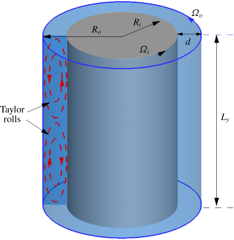
Flow configuration for Taylor–Couette flow with co-rotating cylinders.  $R_{i}$ is the radius of the inner cylinder,
 $R_{o}$ is the radius of the outer cylinder and
 $d=R_{o}-R_{i}$.

Parameters for LES at varying  $Re_{i}$ with
 $\unicode[STIX]{x1D702}=0.909$.
 $N_{\unicode[STIX]{x1D703}}$,
 $N_{r}$ and
 $N_{y}$ are mesh numbers in the azimuthal, radial and spanwise directions, respectively. For all cases, the domain size is a sector
 $\unicode[STIX]{x0394}\unicode[STIX]{x1D703}=\unicode[STIX]{x03C0}/10$ in the azimuthal
 $\unicode[STIX]{x1D703}$ direction and is
 $L_{y}=2\unicode[STIX]{x03C0}d/3$ in the spanwise
 $y$ direction.
 $Re_{\unicode[STIX]{x1D70F}_{i}}=u_{\unicode[STIX]{x1D70F}i}d/2\unicode[STIX]{x1D708}$ as calculated from the LES. Mesh sizes in viscous wall scaling are
 $r_{i}\unicode[STIX]{x0394}\unicode[STIX]{x1D703}^{+}$ and
 $\unicode[STIX]{x0394}y^{+}$ respectively, uniform in both the azimuthal and spanwise directions.
 $\unicode[STIX]{x0394}r_{min}^{+}$ is the minimal near-wall mesh size and
 $\unicode[STIX]{x0394}r_{max}^{+}$ is the maximum mesh size.

3 LES results
3.1 Cases implemented
The geometrical configuration for Taylor–Couette flow is shown in figure 1. In the present LES of Taylor–Couette flow, the outer cylinder is stationary;  $\unicode[STIX]{x1D6FA}_{o}=0$, corresponding to
 $a=-\unicode[STIX]{x1D6FA}_{o}/\unicode[STIX]{x1D6FA}_{i}=0$. The relevant dimensionless parameters defining the flow are then the radius ratio
 $\unicode[STIX]{x1D702}$ and the inner-cylinder Reynolds number
 $Re_{i}$. The inner-cylinder friction Reynolds number is
 $$\begin{eqnarray}Re_{\unicode[STIX]{x1D70F}_{i}}={\displaystyle \frac{u_{\unicode[STIX]{x1D70F}_{i}}d}{2\unicode[STIX]{x1D708}}},\end{eqnarray}$$
where  $u_{\unicode[STIX]{x1D70F}_{i}}=\sqrt{\unicode[STIX]{x1D70F}_{i,w}/\unicode[STIX]{x1D70C}}$ is the inner-cylinder friction velocity, with
 $\unicode[STIX]{x1D70F}_{i,w}$ the shear stress at the wall. Generally, and in experiments, both
 $\unicode[STIX]{x1D702},Re_{i}$ (and
 $a$) are fixed but
 $Re_{\unicode[STIX]{x1D70F}_{i}}$ must be determined by measurement, numerical simulation, theory or modelling. The torque that must be applied to the outer cylinder to sustain the motion is
 $T=2\unicode[STIX]{x03C0}R_{i}^{2}L_{y}\unicode[STIX]{x1D70F}_{i,w}$. In the present LES we use
 $\unicode[STIX]{x1D702}=0.909$ and vary only
 $Re_{i}$. For numerical verification we utilize DNS at
 $Re_{i}$ equal to
 $10^{5}$ and
 $3\times 10^{5}$ (Ostilla-Mónico et al. Reference Ostilla-Mónico, Verzicco, Grossmann and Lohse2016). LES at higher
 $Re_{i}$, up to
 $10^{6}$, are also presented. Parameters for the five LES performed are listed in table 1.
In cylindrical  $(r,\unicode[STIX]{x1D703},y)$ coordinates, the computational domain in each LES is a sector of angle
 $\unicode[STIX]{x03C0}/10$ in the
 $\unicode[STIX]{x1D703}$-direction, which is a well-accepted domain size in DNS simulation by Ostilla-Mónico, Verzicco & Lohse (Reference Ostilla-Mónico, Verzicco and Lohse2015), Ostilla-Mónico et al. (Reference Ostilla-Mónico, Verzicco, Grossmann and Lohse2016). In the spanwise direction the domain length is
 $L_{y}=2\unicode[STIX]{x03C0}d/3$. Periodic boundary conditions are implemented in both
 $\unicode[STIX]{x1D703}$ and
 $y$. The grid resolution in each direction
 $(N_{r},N_{\unicode[STIX]{x1D703}},N_{y})$ is shown in table 1. Grid spacing is uniform in both
 $\unicode[STIX]{x1D703}$ and
 $y$ but is stretched in the
 $r$ direction using a tanh mapping
 $r=R_{i}+d\tanh (\unicode[STIX]{x1D6FE}r_{u})/\tanh (\unicode[STIX]{x1D6FE})$ with
 $r_{u}=[-1,1]$ in order to fulfil the near-wall resolution condition
 $\unicode[STIX]{x0394}r_{min}^{+}\approx 1$ with a restriction on
 $N_{r}$.
The Taylor number, which is defined as (Grossmann et al. Reference Grossmann, Lohse and Sun2016)
 $$\begin{eqnarray}Ta=\frac{(1+\unicode[STIX]{x1D702})^{4}}{64\unicode[STIX]{x1D702}^{2}}\frac{(R_{o}-R_{i})^{2}(R_{o}+R_{i})^{2}(\unicode[STIX]{x1D6FA}_{i}-\unicode[STIX]{x1D6FA}_{o})^{2}}{\unicode[STIX]{x1D708}^{2}},\end{eqnarray}$$
is also shown. Using  $a=-\unicode[STIX]{x1D6FA}_{o}/\unicode[STIX]{x1D6FA}_{i}$ this becomes
 $$\begin{eqnarray}Ta={\displaystyle \frac{(1+\unicode[STIX]{x1D702})^{6}}{64\unicode[STIX]{x1D702}^{4}}}(1+a)^{2}Re_{i}^{2}.\end{eqnarray}$$
Using  $a=0,\unicode[STIX]{x1D702}=0.909$, this is
 $Ta=1.1076Re_{i}^{2}$.
Each LES was started with a coarse mesh and the initial condition comprised of laminar flow. During the flow transition into turbulence, the mesh was refined in stages. Transition was considered completed when the dynamically monitored, instantaneous skin-friction velocities at both inner and outer cylinders reached statistically stationary states. For the purpose of time averaging, each LES was then continued for 2–3 transit times of the inner wall through the computational domain.
For the purpose of defining averaged quantities the flow is assumed to be statistically stationary in time over a sufficiently long time period following initial transients, and spatially homogeneous in the  $\unicode[STIX]{x1D703}$ direction only. In the spanwise direction the flow is generally non-homogenous owing to the presence of Taylor rolls. Starting from a scalar field
 $\unicode[STIX]{x1D719}(r,\unicode[STIX]{x1D703},y,t)$, ‘
 $\hat{..}$’ denotes an average of a space–time-dependent quantity in both time and the azimuthal (
 $\unicode[STIX]{x1D703}$) direction, resulting in
 $\hat{\unicode[STIX]{x1D719}}(r,y)$, while ‘
 $\bar{..}$’ denotes an additional spanwise average of
 $\hat{\unicode[STIX]{x1D719}}(r,y)$, resulting in
 $\overline{\hat{\unicode[STIX]{x1D719}}}(r)$.
The mean velocity in the laboratory frame of reference is  $\boldsymbol{U}(r)\equiv \overline{\hat{\boldsymbol{u}}}$, with components in coordinates
 $(r,\unicode[STIX]{x1D703},y)$ given by
 $(0,U_{\unicode[STIX]{x1D703}}(r),0)$. For the computation of turbulent statistics, a velocity fluctuation is first defined as
 $\boldsymbol{u}^{\prime }(r,\unicode[STIX]{x1D703},y,t)=\boldsymbol{u}(r,\unicode[STIX]{x1D703},y,t)-\hat{\boldsymbol{u}}(r,y)$. Then, the turbulent intensity is computed as
 $R_{\boldsymbol{u}\boldsymbol{u}}=\overline{\widehat{\boldsymbol{u}^{\prime }\boldsymbol{u}^{\prime }}}$. With this definition, for example, the azimuthal turbulence intensity is
 $$\begin{eqnarray}\overline{\widehat{u_{\unicode[STIX]{x1D703}}^{\prime }u_{\unicode[STIX]{x1D703}}^{\prime }}}(r)=\overline{\widehat{u_{\unicode[STIX]{x1D703}}^{2}}(r,y)-\left(\widehat{u_{\unicode[STIX]{x1D703}}}(r,y)\right)^{2}}.\end{eqnarray}$$
In displaying data, both mean-velocity and turbulent intensities are scaled using  $u_{\unicode[STIX]{x1D70F}_{i}}$. With focus on the inner cylinder, following Ostilla-Mónico et al. (Reference Ostilla-Mónico, Verzicco, Grossmann and Lohse2016), we use a scaled and adjusted mean-azimuthal velocity
 $U^{+}=(\unicode[STIX]{x1D6FA}_{i}R_{i}-U_{\unicode[STIX]{x1D703}})/u_{\unicode[STIX]{x1D70F}i}$ and scaled turbulent intensities
 $(u_{j}u_{j})^{+}=R_{u_{j}u_{j}}/u_{\unicode[STIX]{x1D70F}i}^{2}$ with
 $j$ denoting
 $r$,
 $\unicode[STIX]{x1D703}$ or
 $y$. These comprise the one-point turbulent statistics in the present LES study.
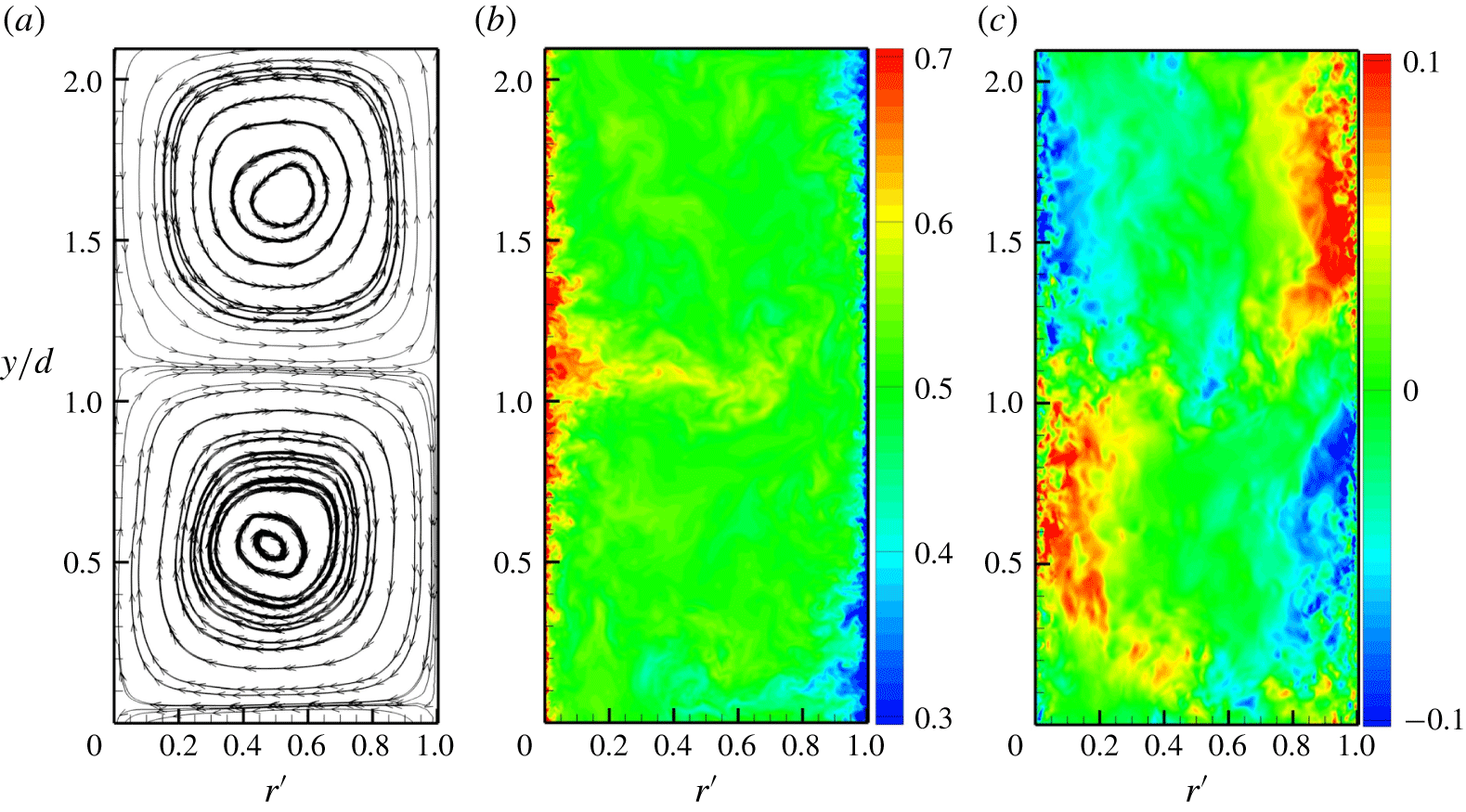
Visualization of an instantaneous flow field in a radial–spanwise plane:  $r^{\prime }=(r-R_{i})/d,y$.
 $Re_{i}=10^{5}$,
 $\unicode[STIX]{x1D702}=0.909$. (a) Streamlines of the azimuthally averaged flow field
 $(u_{r},u_{y})$; (b) instantaneous azimuthal velocity field at a mid-span plane; (c) instantaneous spanwise velocity field at a mid-span plane.

3.2 Verification with DNS at  $Re_{i}=10^{5},3\times 10^{5}$

Verification of our LES is documented using the benchmark DNS of Ostilla-Mónico et al. (Reference Ostilla-Mónico, Verzicco, Grossmann and Lohse2016) at both  $Re_{i}=10^{5}$ and at their highest
 $Re_{i}$ of
 $3\times 10^{5}$. Comparisons mainly include mean-velocity profiles and also turbulent intensities. Figure 2 shows diagnostics of the flow field at
 $Re_{i}=10^{5}$ viewed in an
 $r$-
 $y$ or radial–spanwise plane, where coordinates are scaled using the cylinder gap
 $d$. In the
 $r$ direction, a dimensionless length scale is defined based on the radial distance from the inner cylinder as
 $r^{\prime }=(r-R_{i})/d$. Here,
 $r^{\prime }=0,1$ correspond to the inner rotating cylinder and the outer static cylinder, respectively. Figure 2(a) shows streamlines of the streamwise-averaged, instantaneous flow field in an (
 $r$-
 $y$) plane. One pair of Taylor rolls is observed. The centre and right-hand panels show colour-coded images of the instantaneous azimuthal component
 $u_{\unicode[STIX]{x1D703}}$ and the spanwise velocity component
 $u_{y}$, respectively.
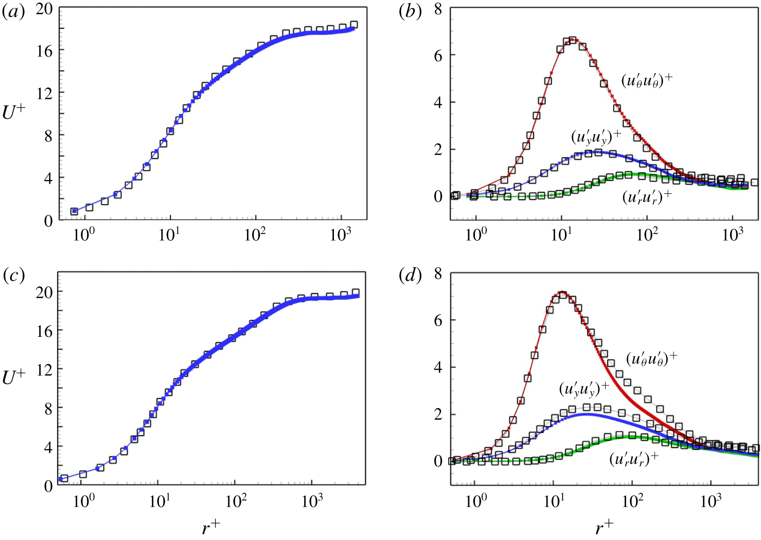
In figure 3, radial profiles of the mean-azimuthal velocity and turbulent intensities are shown for  $Re_{i}=10^{5},3\times 10^{5}$. Both mean and turbulent intensities are scaled with
 $u_{\unicode[STIX]{x1D70F}_{i}}$, with
 $U^{+}$ in the left panels and
 $(u_{\unicode[STIX]{x1D703}}^{\prime }u_{\unicode[STIX]{x1D703}}^{\prime })^{+}$,
 $(u_{y}^{\prime }u_{y}^{\prime })^{+}$ and
 $(u_{r}^{\prime }u_{r}^{\prime })^{+}$ in the right panels versus the scaled length
 $r^{+}=(r-R_{i})/l^{+}$ with
 $l^{+}=\unicode[STIX]{x1D708}/u_{\unicode[STIX]{x1D70F}_{i}}$. The LES mean-velocity profile shows satisfactory agreement with the DNS by Ostilla-Mónico et al. (Reference Ostilla-Mónico, Verzicco, Grossmann and Lohse2016) for both
 $Re_{i}$. A clear log variation is evident in both
 $U^{+}$ versus
 $r^{+}$ plots. The present LES mesh is substantially coarser than required for DNS. For
 $Re_{i}=10^{5}$, the total LES mesh count
 $N=N_{\unicode[STIX]{x1D703}}N_{r}N_{z}$ is
 $1/32$ that of the corresponding DNS, while for
 $Re_{i}=3\times 10^{5}$, this fraction is
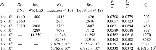
 $1/24$. In table 2 we list values of both
 $Re_{\unicode[STIX]{x1D70F}_{i}}$ and Nusselt number
 $Nu$ for the present LES, in comparison with DNS (Ostilla-Mónico et al. Reference Ostilla-Mónico, Verzicco, Grossmann and Lohse2016).
Comparison of LES with DNS by Ostilla-Mónico et al. (Reference Ostilla-Mónico, Verzicco, Grossmann and Lohse2016). (a) Mean-flow velocity profiles  $U^{+}$ at
 $Re_{i}=10^{5}$; (b) turbulent intensities
 $(u_{\unicode[STIX]{x1D703}}^{\prime }u_{\unicode[STIX]{x1D703}}^{\prime })^{+},(u_{y}^{\prime }u_{y}^{\prime })^{+},(u_{r}^{\prime }u_{r}^{\prime })^{+}$ at
 $Re_{i}=10^{5}$. (c)
 $U^{+}$ at
 $Re_{i}=3\times 10^{5}$; (d) turbulent intensities at
 $Re_{i}=3\times 10^{5}$. Square symbols: DNS by Ostilla-Mónico et al. (Reference Ostilla-Mónico, Verzicco, Grossmann and Lohse2016). Solid lines with filled squares: present LES.

Comparison of skin-friction Reynolds number  $Re_{\unicode[STIX]{x1D70F}_{i}}$ and Nusselt number
 $Nu$ between LES and DNS at varying
 $Re_{i}$ with
 $\unicode[STIX]{x1D702}=0.909$.

3.3 Mean profiles
As shown for TC flows at  $Re_{i}=10^{5}$ and
 $3\times 10^{5}$, the log variation in the velocity profile
 $U^{+}$ persists only in a range of
 $r^{+}$. For large
 $r^{+}$ the mean-azimuthal velocity profile deviates substantially from the log law. Unlike the classical wake profile seen in boundary-layer and pipe flows, this deviation falls below the log line. This can be attributed to the strong spanwise redistribution effect produced by Taylor vortices which results in a central bulk region of almost constant angular momentum. In the estimate of Ostilla-Mónico et al. (Reference Ostilla-Mónico, Verzicco, Grossmann and Lohse2016),
 $r^{+}=0.1Re_{\unicode[STIX]{x1D70F}}$ is considered as an upper bound for the log layer for
 $\unicode[STIX]{x1D702}=0.909$. Mean-velocity profiles
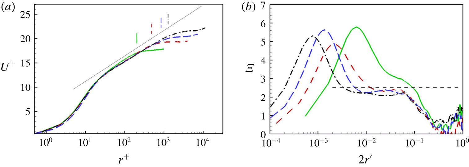
 $U^{+}(r^{+})$ obtained from LES at higher
 $Re_{i}$ are shown in figure 4, which plots five curves, representing the five cases implemented. Also shown is a log profile with
 $\unicode[STIX]{x1D705}=0.42$. Ostilla-Mónico et al. (Reference Ostilla-Mónico, Verzicco and Lohse2015) find that
 $\unicode[STIX]{x1D705}$ obtained from their DNS can depend on both the azimuthal and spanwise domain sizes, with a larger spanwise domain resulting in a somewhat larger
 $\unicode[STIX]{x1D705}$. In figure 4(a), we also plot several vertical lines that indicate the wall-layer thicknesses
 $r_{\unicode[STIX]{x1D6FF}_{i}}^{+}$ predicted by a model to be discussed subsequently. See table 3.
Mean-velocity profiles for all present LES. (a) The mean-azimuthal velocity versus  $r^{+}$; (b), parameter
 $\unicode[STIX]{x1D6EF}$ versus
 $2r^{\prime }$ with
 $r^{\prime }=(r-R_{i})/d$. Lines for different
 $Re_{i}$: ——,
 $10^{5}$, - - - -;
 $3\times 10^{5}$; – – – –
 $6\times 10^{5}$; —⋅—,
 $10^{6}$. Short vertical lines denote the wall-layer thickness
 $r_{\unicode[STIX]{x1D6FF}_{i}}^{+}$ as defined in table 3. A solid line denoting a log profile with Kármán constant
 $\unicode[STIX]{x1D705}=0.42$ is also shown in (a) for comparison.

Model calculations compared with DNS of Ostilla-Mónico et al. (Reference Ostilla-Mónico, Verzicco, Grossmann and Lohse2016) and the present wall-resolved LES,  $a=0$,
 $\unicode[STIX]{x1D702}=0.909$. Two versions of the model calculations for
 $Re_{\unicode[STIX]{x1D70F}_{i}}$ are shown in columns 4 and 5. The predicted outer limit of the log layer,
 $r_{\unicode[STIX]{x1D6FF}_{i}}^{+}=2Re_{\unicode[STIX]{x1D70F}_{i}}\unicode[STIX]{x1D6FF}_{i}/d$ in inner scaling is shown in the last column. For cases corresponding to the present LES, these values are plotted in figure 4(a) as short vertical lines for corresponding
 $Re_{i}$.

Another way to clarify a possible log region is a scaled parameter which is typically defined as
 $$\begin{eqnarray}\unicode[STIX]{x1D6EF}=r^{+}\frac{\text{d}U^{+}}{\text{d}r^{+}}.\end{eqnarray}$$
In the sense of a classic log law,  $\unicode[STIX]{x1D6EF}$ is equal to the inverse of the Kármán constant,
 $1/\unicode[STIX]{x1D705}$. In figure 4(b), we show plots of
 $\unicode[STIX]{x1D6EF}$ for all cases. A horizontal straight line at
 $\unicode[STIX]{x1D6EF}=2.5$ is also shown, corresponding to
 $\unicode[STIX]{x1D705}=0.4$. At our largest
 $Re_{i}$,
 $\unicode[STIX]{x1D6EF}$ is approximately constant over approximately a decade of
 $r^{\prime }$.
3.4 Turbulence intensity profiles
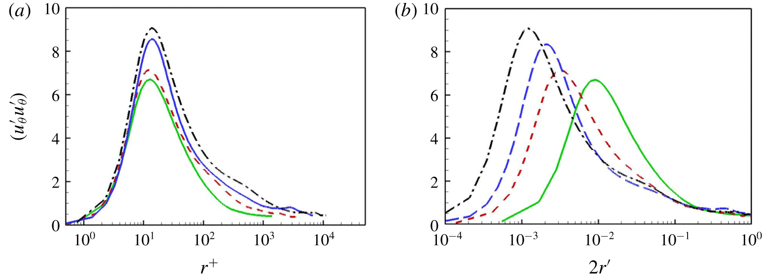
Turbulent intensities  $(u_{\unicode[STIX]{x1D703}}^{\prime }u_{\unicode[STIX]{x1D703}}^{\prime })^{+}$. Lines for different
 $Re_{i}$: ——,
 $10^{5}$; - - - -,
 $3\times 10^{5}$; – – – –,
 $6\times 10^{5}$; —⋅—,
 $10^{6}$. (a) Inner scaling:
 $(u_{\unicode[STIX]{x1D703}}^{\prime }u_{\unicode[STIX]{x1D703}}^{\prime })^{+}$ versus
 $r^{+}$. (b) Outer scaling:
 $(u_{\unicode[STIX]{x1D703}}^{\prime }u_{\unicode[STIX]{x1D703}}^{\prime })^{+}$ versus
 $^{\prime }r^{\prime }=(r-R_{i})/d$.

In figure 5, we show the scaled radial variation of  $(u_{\unicode[STIX]{x1D703}}^{\prime }u_{\unicode[STIX]{x1D703}}^{\prime })^{+}$ using two different length scales. Figure 5(a) uses inner scaling in the form
 $(u_{\unicode[STIX]{x1D703}}^{\prime }u_{\unicode[STIX]{x1D703}}^{\prime })^{+}$ versus
 $r^{+}$, while in figure 5(b), the outer scale
 $r^{\prime }$ is utilized. For the purpose of readability we follow channel flow where
 $2r^{\prime }$ reaches unity at the gap centreline.
When  $(u_{\unicode[STIX]{x1D703}}^{\prime }u_{\unicode[STIX]{x1D703}}^{\prime })^{+}$ is plotted versus
 $r^{+}$, all present LES with
 $\unicode[STIX]{x1D702}=0.909$ show an inner peak, denoted by
 $(u_{\unicode[STIX]{x1D703}}^{\prime }u_{\unicode[STIX]{x1D703}}^{\prime })_{max}^{+}$, at location
 $r_{max}^{+}$, with the latter in the range
 $10<r_{max}^{+}<16$. Further,
 $(u_{\unicode[STIX]{x1D703}}^{\prime }u_{\unicode[STIX]{x1D703}}^{\prime })_{max}^{+}$ shows an increasing tendency with
 $Re_{i}$, or in other words,
 $Re_{\unicode[STIX]{x1D70F}_{i}}$. In figure 5(b), for larger
 $r^{\prime }$,
 $(u_{\unicode[STIX]{x1D703}}^{\prime }u_{\unicode[STIX]{x1D703}}^{\prime })^{+}$ shows a plateau, which extends to the centreline
 $r^{\prime }=1/2$. This behaviour differs from that found in either channel flow or pipe flow. In the latter, streamwise turbulent intensities in the near-centre region, for example
 $y/\unicode[STIX]{x1D6FF}>0.2$ with
 $\unicode[STIX]{x1D6FF}$ the half-height in channel flow and the radius in pipe flow, show monotonically decreasing behaviour in the wall-normal direction away from the wall, approaching a minimum at the centreline. No obvious plateau region is observed. The plateau region of
 $(u_{\unicode[STIX]{x1D703}}^{\prime }u_{\unicode[STIX]{x1D703}}^{\prime })^{+}$ near the centreline region for TC flow can probably be ascribed to turbulent spanwise roll motion, which transports and redistributes angular momentum.
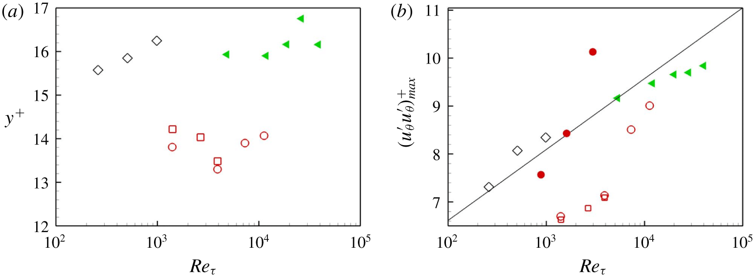
Figure 6(a,b) shows the variation of  $r_{max}^{+}$ and
 $(u_{\unicode[STIX]{x1D703}}^{\prime }u_{\unicode[STIX]{x1D703}}^{\prime })_{max}^{+}$, respectively, versus friction Reynolds number. The present LES results are depicted with the symbol ○. For comparison, DNS results and experimental measurements for TC and plane-Couette flows are shown. Also shown for reference purposes are the pipe flow data of Willert et al. (Reference Willert, Soria, Stanislas, Klinner, Amili, Eisfelder, Cuvier, Bellani, Fiorini and Talamelli2017) and, in figure 6(b), an empirical fitted line
 $(u_{\unicode[STIX]{x1D703}}^{\prime }u_{\unicode[STIX]{x1D703}}^{\prime })_{max}^{+}=3.66+0.642\ln (Re_{\unicode[STIX]{x1D70F}})$ suggested by Lee & Moser (Reference Lee and Moser2015). Here, and in the figure, a generic
 $Re_{\unicode[STIX]{x1D70F}}$ is used to refer to the single friction Reynolds number that characterizes both pipe flow and PC flow and also to the present
 $Re_{\unicode[STIX]{x1D70F}_{i}}$.
(a) Position of peak value of  $(u_{\unicode[STIX]{x1D703}}^{\prime }u_{\unicode[STIX]{x1D703}}^{\prime })^{+}$ versus
 $Re_{\unicode[STIX]{x1D70F}_{i}}$. (b) Peak value
 $(u_{\unicode[STIX]{x1D703}}^{\prime }u_{\unicode[STIX]{x1D703}}^{\prime })_{max}^{+}$ versus
 $Re_{\unicode[STIX]{x1D70F}_{i}}$. ○, Present LES of TC flow. Reference DNS data (hollow symbols): ▫, TC flow by Ostilla-Mónico et al. (Reference Ostilla-Mónico, Verzicco, Grossmann and Lohse2016); ♢, plane-Couette flow by Pirozzoli et al. (Reference Pirozzoli, Bernardini and Orlandi2014). Reference experimental data (filled symbols): ◂, pipe flow by Willert et al. (Reference Willert, Soria, Stanislas, Klinner, Amili, Eisfelder, Cuvier, Bellani, Fiorini and Talamelli2017); ●, TC flow by Huisman et al. (Reference Huisman, Scharnowski, Cierpka, Kähler, Lohse and Sun2013). Dashed line:
 $(u_{\unicode[STIX]{x1D703}}^{\prime }u_{\unicode[STIX]{x1D703}}^{\prime })_{max}^{+}=3.66+0.642\ln [Re_{\unicode[STIX]{x1D70F}}]$ Lee & Moser (Reference Lee and Moser2015).

In wall units, the present LES results do not show a clear tendency for  $r_{max}^{+}$ to move outwards as
 $Re_{\unicode[STIX]{x1D70F}_{i}}$ increases to our largest values. For the two low
 $Re_{i}$ cases, our LES agree well with the DNS of Ostilla-Mónico et al. (Reference Ostilla-Mónico, Verzicco, Grossmann and Lohse2016) (symbol ▫). Their values, around
 $r_{max}^{+}=13.5$, are roughly consistent with the peak location at
 $r^{+}\approx 12$ in TC flow experiments with
 $\unicode[STIX]{x1D702}=0.716$ and
 $Re_{\unicode[STIX]{x1D70F}_{i}}$ up to
 $3200$ (Huisman et al. Reference Huisman, Scharnowski, Cierpka, Kähler, Lohse and Sun2013). Peak locations obtained for pipe flow at
 $Re_{\unicode[STIX]{x1D70F}}$ up to 40 000 by Willert et al. (Reference Willert, Soria, Stanislas, Klinner, Amili, Eisfelder, Cuvier, Bellani, Fiorini and Talamelli2017) (with symbol ◂) also generally reside in this range. In DNS of plane-Couette flow, large-scale rolls are also observed in the spanwise direction. Pirozzoli et al. (Reference Pirozzoli, Bernardini and Orlandi2014) find
 $r_{max}^{+}$ obtained from DNS of plane-Couette flow (symbol ♢) that increases with
 $Re_{\unicode[STIX]{x1D70F}}$, reaching
 $r_{max}^{+}=16.5$ for
 $Re_{\unicode[STIX]{x1D70F}}=1000$.
In figure 6(b) the present LES results for  $(u_{\unicode[STIX]{x1D703}}^{\prime }u_{\unicode[STIX]{x1D703}}^{\prime })_{max}^{+}$ agree quite well with the DNS of Ostilla-Mónico et al. (Reference Ostilla-Mónico, Verzicco, Grossmann and Lohse2016) (symbol ▫) at our lower
 $Re_{\unicode[STIX]{x1D70F}_{i}}$. The LES results show a clear tendency for
 $(u_{\unicode[STIX]{x1D703}}^{\prime }u_{\unicode[STIX]{x1D703}}^{\prime })_{max}^{+}$ to increase with
 $Re_{\unicode[STIX]{x1D70F}_{i}}$. This is broadly consistent with TC flow experiments with
 $\unicode[STIX]{x1D702}=0.716$ and
 $880<Re_{\unicode[STIX]{x1D70F}_{i}}<3200$ (Huisman et al. Reference Huisman, Scharnowski, Cierpka, Kähler, Lohse and Sun2013) (symbol ●). The latter do, however, show a substantially faster increase with
 $Re_{\unicode[STIX]{x1D70F}_{i}}$ than other data or DNS. For boundary-layer flow, Marusic, Mathis & Hutchins (Reference Marusic, Mathis and Hutchins2010) attribute the continued increase of
 $(u_{\unicode[STIX]{x1D703}}^{\prime }u_{\unicode[STIX]{x1D703}}^{\prime })_{max}^{+}$ with friction Reynolds number to an imprint of outer, large-scale energy, possibly associated with very large motion in the outer layer (Kim & Adrian Reference Kim and Adrian1999), on the small-scale, near-wall dynamics. In TC flow, the corresponding outer-flow energy on the scale of the cylinder gap is most likely provided by the action of turbulent Taylor rolls.
In the numerical study of canonical turbulent channel flow (Lee & Moser Reference Lee and Moser2015) or boundary-layer flow (Simens et al. Reference Simens, Jiménez, Hoyas and Mizuno2009), the effect of simulation parameters, such as those associated with the extent of the computational domain and the mesh size, on mean-velocity and turbulent intensity profiles has been carefully studied. For PC flow and TC flow, it is known that spanwise roll motion can strongly impact the zone of wall-bounded turbulence. In order to alleviate spurious effects for PC flow, large computational domains, of order  $30d$ in the streamwise direction and
 $8d$ in the spanwise direction are needed for
 $Re_{\unicode[STIX]{x1D70F}}$ up to
 $1000$ (Pirozzoli et al. Reference Pirozzoli, Bernardini and Orlandi2014), where
 $d$ is the flat-plate gap. Further, according to Lee & Moser (Reference Lee and Moser2018), even longer turbulent structures are observed in plane-Couette flow, which can extend to the entire
 $50\unicode[STIX]{x03C0}d$ domain for
 $Re_{\unicode[STIX]{x1D70F}}=500$. Ostilla-Mónico et al. (Reference Ostilla-Mónico, Verzicco and Lohse2015) investigated the effect of both spanwise and azimuthal domain size on TC flow. They found that finite-domain effects on both the structure of the near-wall log region and on turbulent intensity profiles were generally non-negligible at moderate Reynolds numbers. The issue remains to be resolved.
Finally, we note that, owing to the existence of spanwise roll motion for the present TC flow, the definition of one-point turbulent intensities is not unambiguous. A diagnostic has been used that includes only local small-scale turbulence, and that does not explicitly recognize the presence of large-scale roll motion. According to our present azimuthal intensity metric, a tendency to form a hump and possibly a second peak as the driving Reynolds number increases up to  $Re_{i}=10^{6}$, is not observed. Nor was this found by the DNS of Ostilla-Mónico et al. (Reference Ostilla-Mónico, Verzicco, Grossmann and Lohse2016) with this same metric up to
 $Re_{i}=3\times 10^{5}$ where
 $Re_{\unicode[STIX]{x1D70F}_{i}}=3920$. The detailed study of alternative definitions of turbulent intensity that additionally includes clarification of the effect of domain size is beyond the scope of the present study.
3.5 Angular momentum $L$

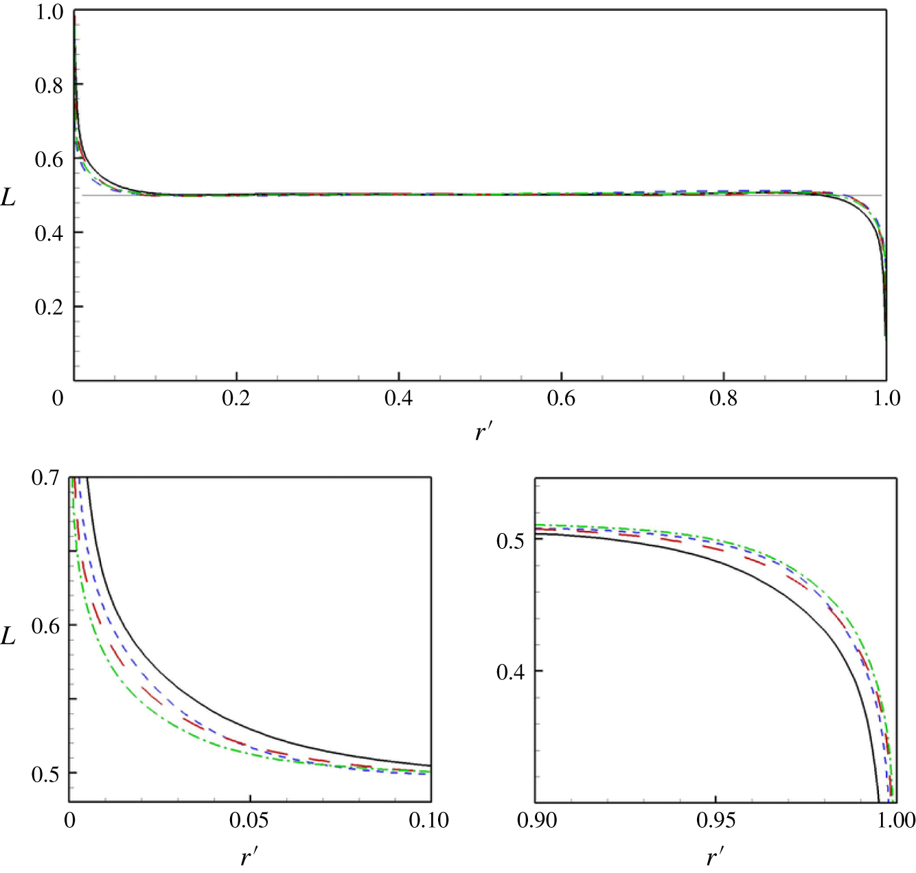
Non-dimensional angular momentum profiles.  $L=rU_{\unicode[STIX]{x1D703}}/(\unicode[STIX]{x1D6FA}_{i}R_{i}^{2})$ lines for different
 $Re_{i}$: ——,
 $10^{5}$; - - - -,
 $3\times 10^{5}$; – – – –,
 $6\times 10^{5}$; —⋅—,
 $10^{6}$.

The presence of Taylor vortices is thought to transport angular momentum per unit mass  $ru_{\unicode[STIX]{x1D703}}$ between the two cylinders, leading to constant angular momentum in the region separating the two cylinder wall layers (Wereley & Lueptow Reference Wereley and Lueptow1999; Ostilla-Mónico et al. Reference Ostilla-Mónico, Verzicco, Grossmann and Lohse2016). The constant is equal to the average of the angular momentum per unit mass of two particles rotating with the angular velocities of both the inner and outer cylinders. For
 $\unicode[STIX]{x1D6FA}_{o}=0$, this is
 $L_{av}=\unicode[STIX]{x1D6FA}_{i}R_{i}^{2}/2$. Figure 7 shows radial profiles of the non-dimensional angular momentum
 $L=rU_{\unicode[STIX]{x1D703}}/(\unicode[STIX]{x1D6FA}_{i}R_{i}^{2})$. A horizontal straight line of
 $L=1/2$ is also plotted for comparison. For all
 $Re_{i}$ shown,
 $L\approx 1/2$ over most of the gap between the two cylinders. The close-up plots near both inner- and outer-cylinder walls in figure 7 show a clear tendency for both wall layers to decrease in thickness relative to the gap width
 $d$, with increasing
 $Re_{i}$.
4 Empirical flow model
4.1 Three-region model
The constancy of angular momentum across the cylinder gap within a region bounded by the two turbulent wall layers adjacent to the cylinder walls suggests a simple empirical mean-flow model of the present TC flow with the outer cylinder stationary. The model development to follow is strictly one-dimensional in the radial direction. While our LES is for an stationary outer cylinder, we develop the model to include both a stationary outer cylinder and a co-rotating cylinder. With  $a=-\unicode[STIX]{x1D6FA}_{o}/\unicode[STIX]{x1D6FA}_{i}$, co-rotation corresponds to
 $a<0$. The model requires that the central region have constant mean angular momentum equal to the average of that associated with the angular velocities of the inner and outer cylinders. The DNS of Ostilla-Mónico et al. (Reference Ostilla-Mónico, van der Poel, Verzicco, Grossmann and Lohse2014) provides some evidence for this for co-rotating TC flow with
 $a=-0.2$. Their figure 4(a) plots
 $(U_{\unicode[STIX]{x1D703}}/r-\unicode[STIX]{x1D6FA}_{o})/(\unicode[STIX]{x1D6FA}_{i}-\unicode[STIX]{x1D6FA}_{o})$ versus
 $r^{\prime }$ for various values of
 $a$. These plots can be converted to angular momentum
 $L$ versus
 $r^{\prime }$. The case
 $a=-0.2$ shows an almost constant angular momentum zone with
 $L$ the average of the inner- and outer-cylinder values. This provides some confidence in extending the present model to the co-rotating case.
The presence of three distinct regions corresponding to wall layers and a central bulk core has been discussed for both Rayleigh–Bénard and Taylor–Couette flows (Chavanne et al. Reference Chavanne, Chilla, Castaing, Hebral, Chabaud and Chaussy1997; Grossmann & Lohse Reference Grossmann and Lohse2011; Grossmann et al. Reference Grossmann, Lohse and Sun2016; Ostilla-Mónico et al. Reference Ostilla-Mónico, Verzicco, Grossmann and Lohse2016). The radial domain  $R_{i}\leqslant r\leqslant R_{o}$ is first divided into three regions, denoted I, II, III. In regions I and III the azimuthal mean flow is modelled as wall layers represented by log-like profiles relative to the wall while, in the central region,
 $U_{\unicode[STIX]{x1D703}}$ corresponds to radially constant angular momentum. The dimensions and mean-velocity profiles in the laboratory frame are then given by
(I)
$R_{i}\leqslant r\leqslant R_{i}+\unicode[STIX]{x1D6FF}_{i}$ with mean-azimuthal velocity: (4.1)$$\begin{eqnarray}U_{\unicode[STIX]{x1D703}}=\unicode[STIX]{x1D6FA}_{i}R_{i}-u_{\unicode[STIX]{x1D70F}_{i}}\left(\frac{1}{\unicode[STIX]{x1D705}}\ln \left(\frac{(r-R_{i})u_{\unicode[STIX]{x1D70F}_{i}}}{\unicode[STIX]{x1D708}}\right)+A\right).\end{eqnarray}$$(II)
$R_{i}+\unicode[STIX]{x1D6FF}_{i}\leqslant r\leqslant R_{o}-\unicode[STIX]{x1D6FF}_{o}$ with mean-azimuthal velocity corresponding to constant angular momentum (4.2)$$\begin{eqnarray}U_{\unicode[STIX]{x1D703}}={\displaystyle \frac{1}{2r}}\left(\unicode[STIX]{x1D6FA}_{i}R_{i}^{2}+\unicode[STIX]{x1D6FA}_{o}R_{o}^{2}\right).\end{eqnarray}$$(III)
$R_{o}-\unicode[STIX]{x1D6FF}_{o}\leqslant r\leqslant R_{o}$ with mean-azimuthal velocity (4.3)Here,$$\begin{eqnarray}U_{\unicode[STIX]{x1D703}}=\unicode[STIX]{x1D6FA}_{o}R_{o}+u_{\unicode[STIX]{x1D70F}_{o}}\left(\frac{1}{\unicode[STIX]{x1D705}}\ln \left(\frac{(R_{o}-r)u_{\unicode[STIX]{x1D70F}_{o}}}{\unicode[STIX]{x1D708}}\right)+A\right).\end{eqnarray}$$$u_{\unicode[STIX]{x1D70F}_{i}}$, $u_{\unicode[STIX]{x1D70F}_{o}}$ are friction speeds at the inner/outer cylinder surfaces, $\unicode[STIX]{x1D6FF}_{i}$, $\unicode[STIX]{x1D6FF}_{o}$ are, respectively, the thicknesses of the inner- and outer-cylinder wall layers and $\unicode[STIX]{x1D705}$ and $A$ are the Kármán constant and turbulent boundary-layer offset parameter, respectively. The model replaces the wake region, present in pipe and boundary-layer flows, by a central zone of constant but known azimuthal velocity corresponding to constant angular momentum. Subsequently, we will refer to the model log-like regions as ‘wall layers’.





For given  $\unicode[STIX]{x1D6FA}_{i},\unicode[STIX]{x1D6FA}_{o},R_{i},R_{o}$ and
 $\unicode[STIX]{x1D708}$, there are four unknowns:
 $(u_{\unicode[STIX]{x1D70F}_{i}},u_{\unicode[STIX]{x1D70F}_{o}},\unicode[STIX]{x1D6FF}_{i},\unicode[STIX]{x1D6FF}_{o})$. Two equations can be obtained by matching
 $U_{\unicode[STIX]{x1D703}}$ at
 $r=R_{i}+\unicode[STIX]{x1D6FF}_{i}$ and
 $r=R_{i}-\unicode[STIX]{x1D6FF}_{o}$. A third is the relation, obtained by equality of the magnitudes of the torques exerted at each cylinder surface on the fluid
 $$\begin{eqnarray}u_{\unicode[STIX]{x1D70F}_{o}}=\unicode[STIX]{x1D702}u_{\unicode[STIX]{x1D70F}_{i}}.\end{eqnarray}$$
The velocity matching equations are
 $$\begin{eqnarray}\displaystyle & \displaystyle \unicode[STIX]{x1D6FA}_{i}R_{i}-u_{\unicode[STIX]{x1D70F}_{i}}\left(\frac{1}{\unicode[STIX]{x1D705}}\ln \left(\frac{\unicode[STIX]{x1D6FF}_{i}u_{\unicode[STIX]{x1D70F}_{i}}}{\unicode[STIX]{x1D708}}\right)+A\right)-{\displaystyle \frac{\unicode[STIX]{x1D6FA}_{i}R_{i}^{2}+\unicode[STIX]{x1D6FA}_{o}R_{o}^{2}}{2(R_{i}+\unicode[STIX]{x1D6FF}_{i})}}=0, & \displaystyle\end{eqnarray}$$
 $$\begin{eqnarray}\displaystyle & \displaystyle \unicode[STIX]{x1D702}u_{\unicode[STIX]{x1D70F}_{i}}\left(\frac{1}{\unicode[STIX]{x1D705}}\ln \left(\frac{\unicode[STIX]{x1D6FF}_{o}\unicode[STIX]{x1D702}u_{\unicode[STIX]{x1D70F}_{i}}}{\unicode[STIX]{x1D708}}\right)+A\right)-{\displaystyle \frac{\unicode[STIX]{x1D6FA}_{i}R_{i}^{2}+\unicode[STIX]{x1D6FA}_{o}R_{o}^{2}}{2(R_{o}-\unicode[STIX]{x1D6FF}_{o})}}=0, & \displaystyle\end{eqnarray}$$
where (4.4) has been used in (4.6). It is noted that this gives a gradient discontinuity at both radial matching locations. Continuity of the azimuthal velocity derivative would perhaps require the addition of intermediate matching regions. While more physically realistic we would expect such extended modelling to add substantial complexity compared to the present model. For our purposes, it will be sufficient to consider (4.5), which is one equation for the two unknowns  $(u_{\unicode[STIX]{x1D70F}_{i}},\unicode[STIX]{x1D6FF}_{i})$. A closure relation is required.
The present LES shows turbulent wall layers that are confined, probably by the action of the spanwise motion associated with Taylor vortices balancing wall-normal turbulent diffusion. Further, the LES indicates an inner-cylinder wall-layer thickness that decreases on the gap scale  $d$, with increasing
 $Re_{i}$; see figure 7. In order to obtain a closure relationship, we consider an analogy with confined viscous layers in laminar wall layers subject to an external lateral straining motion or to Kármán-type swirling flows, where an equilibrium layer thickness scales as
 $\unicode[STIX]{x1D6FF}\sim (\unicode[STIX]{x1D708}/\unicode[STIX]{x1D6FE})^{1/2}$, where
 $\unicode[STIX]{x1D6FE}$ is an imposed outer strain rate or swirl angular velocity. Here, we take
 $\unicode[STIX]{x1D6FE}\sim \unicode[STIX]{x1D6FA}_{i}$,
 $\unicode[STIX]{x1D6FF}\rightarrow \unicode[STIX]{x1D6FF}_{i}$ and utilize an eddy viscosity for large turbulent eddies
 $\unicode[STIX]{x1D708}_{T}\sim \unicode[STIX]{x1D6FF}_{i}u_{\unicode[STIX]{x1D70F}_{i}}$. This gives
 $$\begin{eqnarray}\unicode[STIX]{x1D6FF}_{i}=K\frac{u_{\unicode[STIX]{x1D70F}_{i}}}{\unicode[STIX]{x1D6FA}_{i}},\end{eqnarray}$$
where  $K$ is a dimensionless constant independent of
 $\unicode[STIX]{x1D702}$. Equation (4.7) can be expressed in a dimensionless form as
 $$\begin{eqnarray}\frac{\unicode[STIX]{x1D6FF}_{i}}{d}=\unicode[STIX]{x1D6FC}{\displaystyle \frac{Re_{\unicode[STIX]{x1D70F}_{i}}}{Re_{i}}}{\displaystyle \frac{\unicode[STIX]{x1D702}}{1-\unicode[STIX]{x1D702}}},\end{eqnarray}$$
where  $\unicode[STIX]{x1D6FC}=2K$ and
 $R_{i}=d\unicode[STIX]{x1D702}/(1-\unicode[STIX]{x1D702})$ has been used. Next, substitute (4.8) into (4.5) to obtain a single equation for
 $Re_{\unicode[STIX]{x1D70F}_{i}}$ when other parameters are specified. After some algebra, this can be expressed in non-dimensional form as
 $$\begin{eqnarray}\displaystyle & & \displaystyle \left(1+\frac{a}{\unicode[STIX]{x1D702}^{2}}\right)Re_{i}^{2}-4\unicode[STIX]{x1D6FC}ARe_{\unicode[STIX]{x1D70F}_{i}}^{2}+2(\unicode[STIX]{x1D6FC}-2A)Re_{i}Re_{\unicode[STIX]{x1D70F}_{i}}\nonumber\\ \displaystyle & & \displaystyle \qquad -\,\frac{4}{\unicode[STIX]{x1D705}}Re_{\unicode[STIX]{x1D70F}_{i}}(Re_{i}+\unicode[STIX]{x1D6FC}Re_{\unicode[STIX]{x1D70F}_{i}})\ln \left(\frac{2\unicode[STIX]{x1D6FC}\unicode[STIX]{x1D702}Re_{\unicode[STIX]{x1D70F}_{i}}^{2}}{Re_{i}(1-\unicode[STIX]{x1D702})}\right)=0.\end{eqnarray}$$
In (4.9)  $\unicode[STIX]{x1D705},A$ can be chosen via standard log-law parameters but
 $\unicode[STIX]{x1D6FC}$ is a model-dependent parameter. When these are specified together with
 $\unicode[STIX]{x1D702}$ and
 $Re_{i}$, equation (4.9) can be solved numerically for
 $Re_{\unicode[STIX]{x1D70F}_{i}}$. Then
 $\unicode[STIX]{x1D6FF}_{i}/d$ can be calculated from (4.8). Once the parameters of the inner-cylinder wall layer are known, then (4.6) can be used to determine the single remaining parameter
 $\unicode[STIX]{x1D6FF}_{o}/d$.
In the sequel, canonical values  $A=4.5$,
 $\unicode[STIX]{x1D705}=0.4$ will be chosen. Ostilla-Mónico et al. (Reference Ostilla-Mónico, Verzicco, Grossmann and Lohse2016) find
 $Re_{\unicode[STIX]{x1D70F}_{i}}=1410$ with
 $\unicode[STIX]{x1D702}=0.909$,
 $Re_{i}=10^{5}$. Solving (4.9) with these parameters and with
 $\unicode[STIX]{x1D6FC}=0.25,0.5,0.75,1.0$ gives
 $Re_{\unicode[STIX]{x1D70F}_{i}}=1529,1418,1360,1323$ respectively. For all subsequent calculations with the present model, we will use
 $\unicode[STIX]{x1D6FC}=0.5$, which gives satisfactory agreement with DNS for this case. Setting
 $\unicode[STIX]{x1D6FC}=1/2$ in (4.9) leads to our basic model equation
 $$\begin{eqnarray}\displaystyle & & \displaystyle \left(1+\frac{a}{\unicode[STIX]{x1D702}^{2}}\right)Re_{i}^{2}-2ARe_{\unicode[STIX]{x1D70F}_{i}}^{2}+(1-4A)Re_{i}Re_{\unicode[STIX]{x1D70F}_{i}}\nonumber\\ \displaystyle & & \displaystyle \qquad -\,\frac{2}{\unicode[STIX]{x1D705}}Re_{\unicode[STIX]{x1D70F}_{i}}(2Re_{i}+Re_{\unicode[STIX]{x1D70F}_{i}})\ln \left(\frac{\unicode[STIX]{x1D702}Re_{\unicode[STIX]{x1D70F}_{i}}^{2}}{Re_{i}(1-\unicode[STIX]{x1D702})}\right)=0.\end{eqnarray}$$
According to the structure of the model, the presence of a uniform angular momentum zone separating the two wall layers means that these behave somewhat independently but are connected by (4.4). This decoupling implies that, for the purpose of modelling the inner wall layer, an explicit outer wall-layer mean-flow model is not strictly required. It is included presently for completeness. The determination of  $u_{\unicode[STIX]{x1D70F}_{o}}$ is fixed by (4.4), which is model independent. For the present outer wall model, the calculation of
 $\unicode[STIX]{x1D6FF}_{o}$ is straightforward. Details are given in appendix A, where it is shown that, for the present range of parameters, to two or three significant digits,
 $\unicode[STIX]{x1D6FF}_{o}=\unicode[STIX]{x1D6FF}_{i}/\unicode[STIX]{x1D702}$.
4.2 Approximate analytical solution
Equation (4.10) is not solvable in terms of standard special functions. Ostilla-Mónico et al. (Reference Ostilla-Mónico, Verzicco, Grossmann and Lohse2016) report  $Re_{\unicode[STIX]{x1D70F}_{i}}=1410$ at
 $Re_{i}=10^{5}$ and
 $Re_{\unicode[STIX]{x1D70F}_{i}}=3920$ at
 $Re_{i}=3\times 10^{5}$, giving
 $Re_{\unicode[STIX]{x1D70F}_{i}}/Re_{i}=0.0141,0.0131$ respectively. This suggest the useful approximation
 $Re_{\unicode[STIX]{x1D70F}_{i}}\ll Re_{i}$. According to the present model, this can be shown to improve with increasing
 $Re_{i}$. Neglecting the
 $Re_{\unicode[STIX]{x1D70F}_{i}}^{2}$ term and also the
 $Re_{\unicode[STIX]{x1D70F}_{i}}^{2}$ term multiplying the
 $\ln$ and dividing by
 $Re_{i}$ leads to
 $$\begin{eqnarray}\left(1+\frac{a}{\unicode[STIX]{x1D702}^{2}}\right)Re_{i}+Re_{\unicode[STIX]{x1D70F}_{i}}(1-4A)-\frac{4}{\unicode[STIX]{x1D705}}Re_{\unicode[STIX]{x1D70F}_{i}}\ln \left(\frac{\unicode[STIX]{x1D702}Re_{\unicode[STIX]{x1D70F}_{i}}^{2}}{Re_{i}(1-\unicode[STIX]{x1D702})}\right)=0.\end{eqnarray}$$
This reduction is supported by inspection of the numerical order of magnitude of all terms in (4.10) for solutions with parameters in the present range of interest. This (not shown) indicates that the neglected terms are subdominant. Equation (4.11) will be shown to provide a good analytical approximation to exact numerical solutions of (4.10) over the range of parameters considered presently.
Equation (4.11) has the analytic solution
 $$\begin{eqnarray}\displaystyle Re_{\unicode[STIX]{x1D70F}_{i}}(Re_{i},\unicode[STIX]{x1D702},a) & = & \displaystyle \frac{\unicode[STIX]{x1D705}\left(1+{\displaystyle \frac{a}{\unicode[STIX]{x1D702}^{2}}}\right)Re_{i}}{8W(Z_{1})},\nonumber\\ \displaystyle Z_{1} & = & \displaystyle \frac{\unicode[STIX]{x1D705}\left(1+{\displaystyle \frac{a}{\unicode[STIX]{x1D702}^{2}}}\right)\unicode[STIX]{x1D702}^{1/2}Re_{i}^{1/2}\exp [\unicode[STIX]{x1D705}(4A-1)/8]}{8(1-\unicode[STIX]{x1D702})^{1/2}},\end{eqnarray}$$
where  $W(Z)$ is the principal branch of the Lambert (or ProductLog) function, defined as the inverse of
 $Z=W\ln W$. The
 $W$-function often appears in solutions for the wall friction velocity in wall-bounded flows, see for example Grossmann & Lohse (Reference Grossmann and Lohse2011). The Lambert function is sub-logarithmic, with expansion for large
 $Z$ (Corless et al. Reference Corless, Gonnet, Hare, Jeffrey and Knuth1996)
 $$\begin{eqnarray}\displaystyle W(Z) & = & \displaystyle L_{1}-L_{2}+{\displaystyle \frac{L_{2}}{L_{1}}}+{\displaystyle \frac{L_{2}(-2+L_{2})}{2L_{1}^{2}}}+{\displaystyle \frac{L_{2}(-6-9L_{2}+2L_{2}^{2})}{6L_{1}^{3}}}\nonumber\\ \displaystyle & & \displaystyle +\,{\displaystyle \frac{L_{2}(-12+36L_{2}-22L_{2}^{2}+3L_{2}^{3})}{12L_{1}^{4}}}+O\left(\left({\displaystyle \frac{L_{2}}{L_{1}}}\right)^{6}\right),\nonumber\\ \displaystyle & & \displaystyle L_{1}=\ln (Z),\quad L_{2}=\ln (\ln (Z)).\end{eqnarray}$$
For  $a=0$, results are shown in table 3 for comparison with the DNS of Ostilla-Mónico et al. (Reference Ostilla-Mónico, Verzicco, Grossmann and Lohse2016) and also with the results of the present wall-resolved LES. Results using both (4.10) and (4.12) are shown, where differences in calculated values of
 $Re_{\unicode[STIX]{x1D70F}_{i}}$ are less than 0.5 %. Other values of
 $\unicode[STIX]{x1D702}$ in the range
 $0.5-0.91$ show similar errors in the approximate versus exact numerical model estimates of
 $Re_{\unicode[STIX]{x1D70F}_{i}}(\unicode[STIX]{x1D702},Re_{i})$. Also shown are calculations for both
 $\unicode[STIX]{x1D6FF}_{o}/d$ and
 $\unicode[STIX]{x1D6FF}_{i}/d$, where
 $\unicode[STIX]{x1D6FF}_{o}=\unicode[STIX]{x1D6FF}_{i}/\unicode[STIX]{x1D702}$. Equations (4.12) and (4.8) show that
 $\unicode[STIX]{x1D6FF}_{i}/d$ decreases slowly with increasing
 $Re_{\unicode[STIX]{x1D70F}_{i}}$ as the reciprocal of the Lambert function with an argument proportional to
 $Re_{\unicode[STIX]{x1D70F}_{i}}^{1/2}$. The right-hand column of table 3 shows the model estimate of the extent of the wall log layer, expressed in viscous wall units as
 $r_{\unicode[STIX]{x1D6FF}_{i}}^{+}=2Re_{\unicode[STIX]{x1D70F}_{i}}\unicode[STIX]{x1D6FF}_{i}/d$. These values are shown as short vertical lines in figure 4(a).
4.3 Nusselt number approximation
The Taylor number is defined by equation (3.3). The Nusselt number  $Nu$ is defined as the ratio of the torque required to sustain a statistical steady state of turbulent motion to the torque required for strictly laminar viscous motion at the same
 $Re_{i}$ (Grossmann et al. Reference Grossmann, Lohse and Sun2016). Using the viscous flow solution and the definition of
 $u_{\unicode[STIX]{x1D70F}_{i}}^{2}=\unicode[STIX]{x1D70F}_{w,i}/\unicode[STIX]{x1D70C}$,
 $Nu$ can be expressed as
 $$\begin{eqnarray}Nu=\frac{2\unicode[STIX]{x1D702}(1+\unicode[STIX]{x1D702})Re_{\unicode[STIX]{x1D70F}_{i}}^{2}}{(1+a)Re_{i}}.\end{eqnarray}$$
Hence, for given  $\unicode[STIX]{x1D702},a$ and
 $Re_{i}$, if
 $Re_{\unicode[STIX]{x1D70F}_{i}}$ is known from a solution to (4.10), then both
 $Ta$ and
 $N_{u}$ can be calculated. Alternatively, when (4.12) is combined with (4.14), this gives
 $$\begin{eqnarray}\displaystyle & \displaystyle Nu(Ta,\unicode[STIX]{x1D702},a)=\frac{\unicode[STIX]{x1D705}^{2}(a+\unicode[STIX]{x1D702}^{2})^{2}Ta^{1/2}}{4(1+a)^{2}\unicode[STIX]{x1D702}(1+\unicode[STIX]{x1D702})^{2}(W(Z_{2}))^{2}}, & \displaystyle\end{eqnarray}$$
 $$\begin{eqnarray}\displaystyle & \displaystyle Z_{2}=\frac{\unicode[STIX]{x1D705}(a+\unicode[STIX]{x1D702}^{2})Ta^{1/4}\exp [\unicode[STIX]{x1D705}(4A-1)/8]}{2^{3/2}(1+a)^{1/2}\unicode[STIX]{x1D702}^{1/2}(1-\unicode[STIX]{x1D702})^{1/2}(1+\unicode[STIX]{x1D702})^{3/2}}. & \displaystyle\end{eqnarray}$$
Specific calculations show that, for the range of  $\unicode[STIX]{x1D702}$ and
 $Ta$ considered currently, numerical solutions of (4.10) together with (4.14) agree with (4.15) to 1 % or better, improving with increasing
 $Ta$.
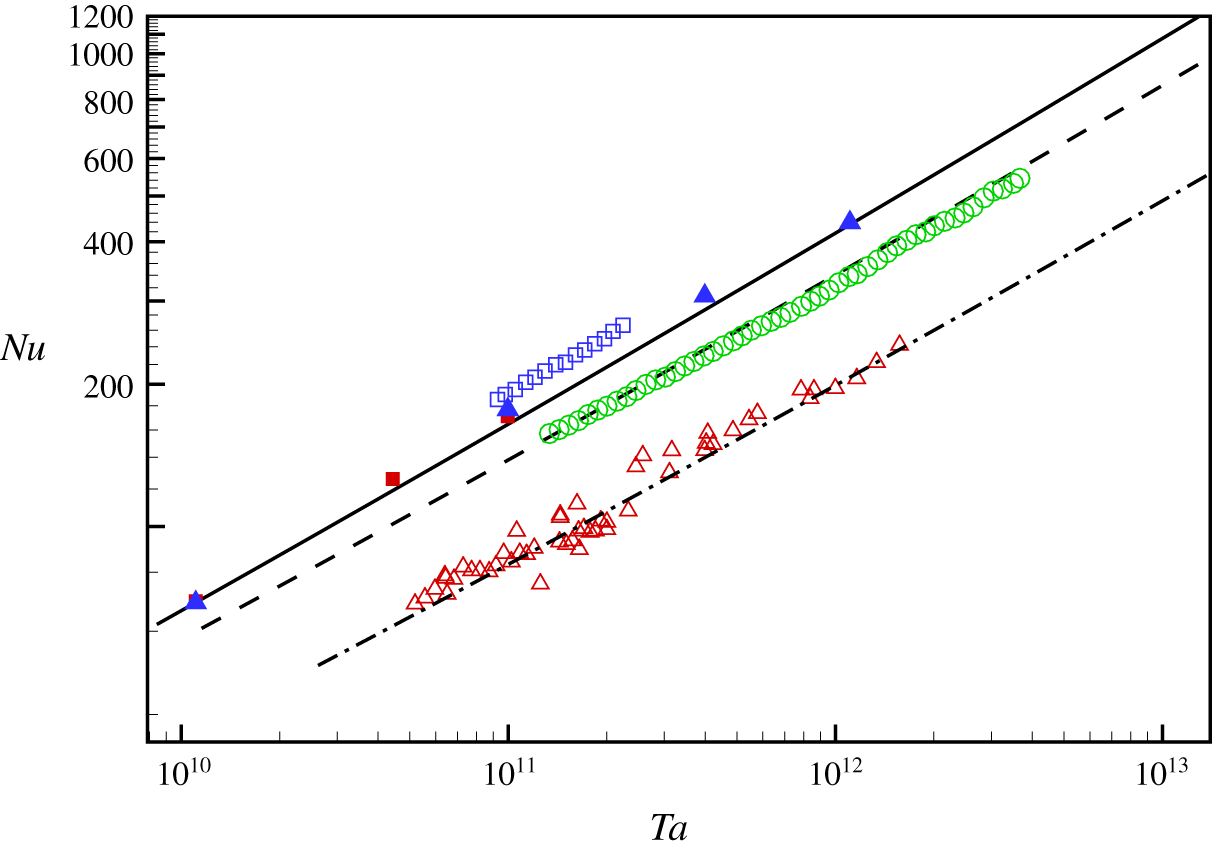
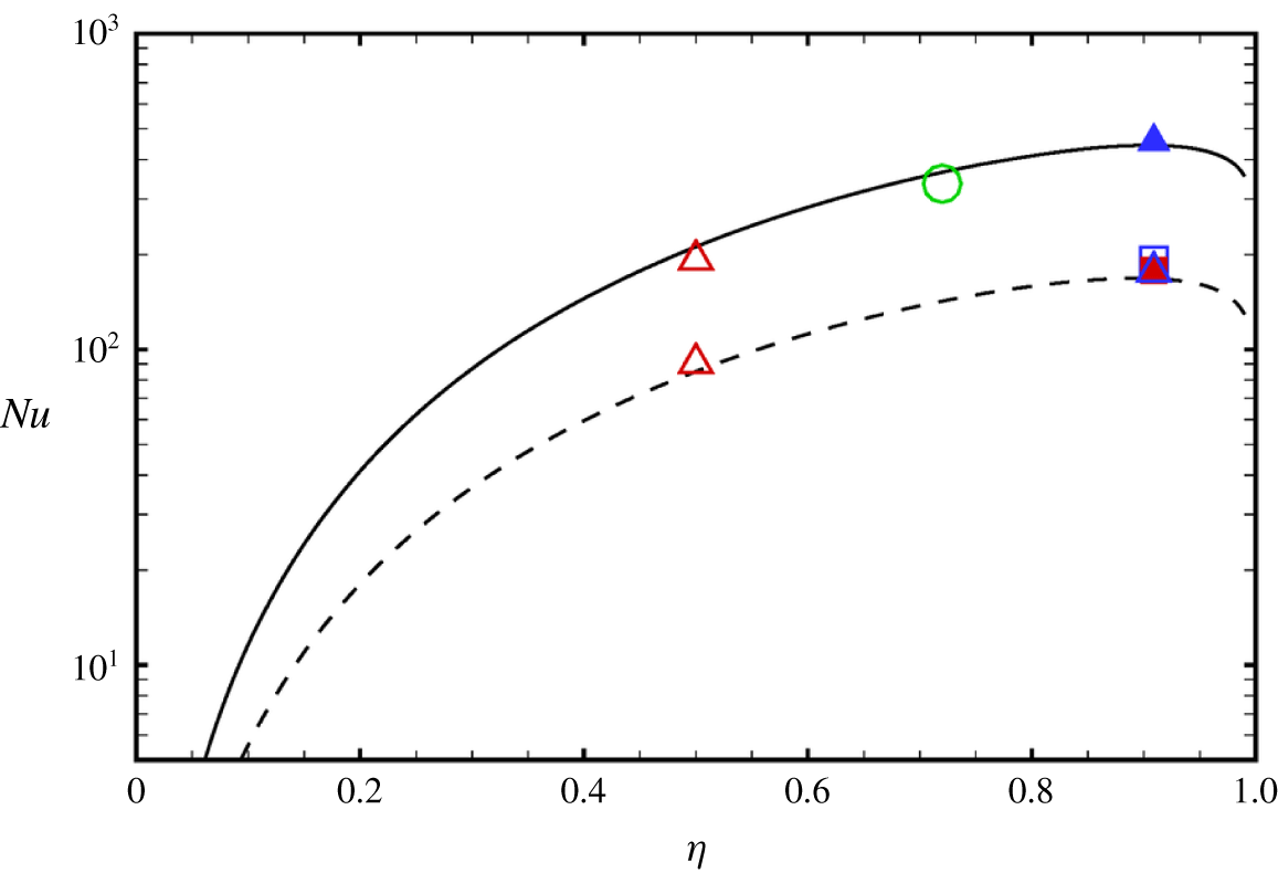
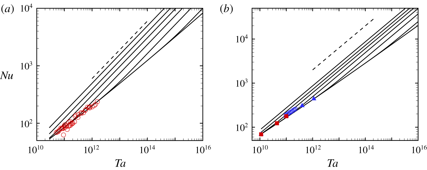
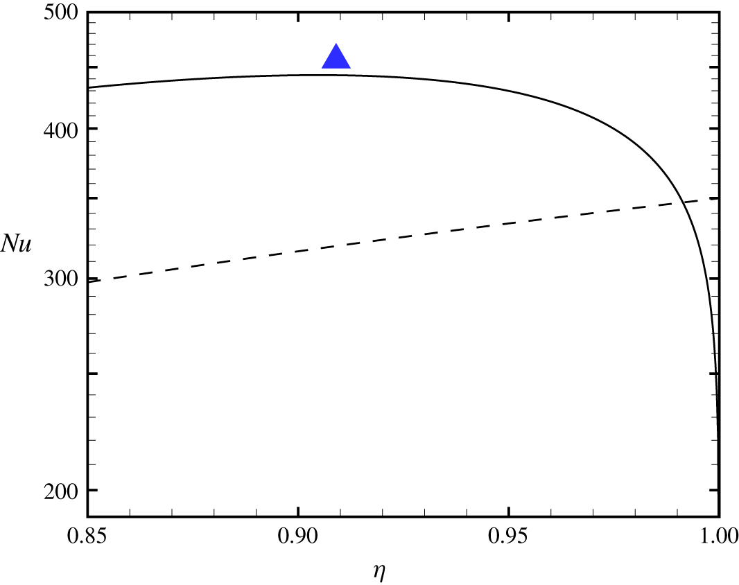
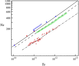
Figure 8 shows  $Nu$ verses
 $Ta$ for
 $a=0$,
 $\unicode[STIX]{x1D702}$ fixed using (4.15) compared with DNS of Ostilla-Mónico et al. (Reference Ostilla-Mónico, Verzicco, Grossmann and Lohse2016), our wall-resolved LES for
 $\unicode[STIX]{x1D702}=0.909$ and with data for
 $\unicode[STIX]{x1D702}=0.5,0.72,0.909$ (Merbold et al. Reference Merbold, Brauckmann and Egbers2013; Van Gils et al. Reference Van Gils, Huisman, Bruggert, Sun and Lohse2011, Reference Van Gils, Huisman, Grossmann, Sun and Lohse2012) obtained from Grossmann et al. (Reference Grossmann, Lohse and Sun2016), while figure 9 shows
 $Nu$ versus
 $\unicode[STIX]{x1D702}$ for two values of
 $Ta=10^{11},10^{12}$. The model captures well the dependence of
 $Nu(Ta,\unicode[STIX]{x1D702})$ on both
 $Ta$ and
 $\unicode[STIX]{x1D702}$ over the range shown. The decrease of
 $Nu$ with
 $\unicode[STIX]{x1D702}$ larger than approximately
 $\unicode[STIX]{x1D702}=0.91$ is surprising. When
 $\unicode[STIX]{x1D702}\rightarrow 1$, the turbulent flow is expected to be similar to plane-Couette flow. Substitution of (4.12) into (4.8) gives
 $\unicode[STIX]{x1D6FF}_{i}/d$ as a function of
 $(Re_{i},\unicode[STIX]{x1D702},a)$, which can be converted to
 $(Ta,\unicode[STIX]{x1D702},a)$. At fixed
 $Ta$ in the present range of interest, and with
 $a=0$, it is found that both
 $\unicode[STIX]{x1D6FF}_{i}/d$,
 $\unicode[STIX]{x1D6FF}_{o}/d$ rapidly increase until a limit is reached where
 $\unicode[STIX]{x1D6FF}_{i}+\unicode[STIX]{x1D6FF}_{o}=d$. This means that the wall layers occupy the entire gap with the extent of the angular momentum zone reducing to zero. This may be taken as defining limits on the validity of the present three-region model. For
 $a=0$,
 $Ta=10^{10},10^{12},10^{14},10^{16}$ it is found that the limit values are
 $\unicode[STIX]{x1D702}=0.98867,0.99084,0.99234,0.99342$ respectively. For
 $\unicode[STIX]{x1D702}$ greater than these values, an alternative model may be more appropriate, for example two wall layers that meet near the gap centre (Grossmann & Lohse Reference Grossmann and Lohse2011). This is discussed in more detail in appendix B. We know of no TC DNS or experimental data in this range of
 $\unicode[STIX]{x1D702}$.
Value of  $Nu$ versus
 $Ta$. Open symbols; experiment
 $\unicode[STIX]{x1D702}=0.909$ (▫),
 $0.72$ (○) Van Gils et al. (Reference Van Gils, Huisman, Bruggert, Sun and Lohse2011, Reference Van Gils, Huisman, Grossmann, Sun and Lohse2012);
 $\unicode[STIX]{x1D702}=0.5$ (▵) Merbold et al. (Reference Merbold, Brauckmann and Egbers2013). ▪; DNS of
 $\unicode[STIX]{x1D702}=0.909$ by Ostilla-Mónico et al. (Reference Ostilla-Mónico, Verzicco, Grossmann and Lohse2016). ▴; present LES of
 $\unicode[STIX]{x1D702}=0.909$. Lines: from (4.15).——,
 $\unicode[STIX]{x1D702}=0.909$. - - - -;
 $\unicode[STIX]{x1D702}=0.72$. —⋅—;
 $\unicode[STIX]{x1D702}=0.5$.

Value of  $Nu$ versus
 $\unicode[STIX]{x1D702}$,
 $a=0$. Dashed line
 $Ta=10^{11}$. Solid line
 $Ta=1.108\times 10^{12}$. Symbols key; see figure 8.

It is clear from the analytic form and the known behaviour of the Lambert function, that  $Nu(\unicode[STIX]{x1D702},Ta)$ with
 $\unicode[STIX]{x1D702}$ fixed increases more slowly than
 $Ta^{1/2}$. Using (4.13), (4.15) with
 $a=0$ has the leading-order asymptotic form
 $$\begin{eqnarray}Nu(Ta,\unicode[STIX]{x1D702})=\frac{\unicode[STIX]{x1D705}^{2}\unicode[STIX]{x1D702}^{3}Ta^{1/2}}{4(1+\unicode[STIX]{x1D702})^{2}(\ln (Z_{3})-\ln (\ln (Z_{3})))^{2}}+HOT,\end{eqnarray}$$
with ‘HOT’ denoting high-order term. For gigantic  $Ta$, this becomes
 $$\begin{eqnarray}Nu(Ta,\unicode[STIX]{x1D702})=\frac{4\unicode[STIX]{x1D705}^{2}\unicode[STIX]{x1D702}^{3}Ta^{1/2}}{(1+\unicode[STIX]{x1D702})^{2}(\ln [Ta])^{2}}+HOT.\end{eqnarray}$$
Equation (4.18) is not a useful practical approximation to (4.15) at  $Ta$ typical of the highest
 $Ta$ experimental data.
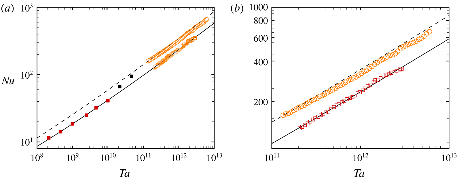
In figure 10 results using (4.15) are compared with the experimental results of Van Gils et al. (Reference Van Gils, Huisman, Bruggert, Sun and Lohse2011, Reference Van Gils, Huisman, Grossmann, Sun and Lohse2012) and DNS of Ostilla-Mónico et al. (Reference Ostilla-Mónico, van der Poel, Verzicco, Grossmann and Lohse2014) for  $\unicode[STIX]{x1D702}=0.714$ and
 $a=0,-0.2$. Figure 10(b) is a magnification over
 $10^{11}\leqslant Ta\leqslant 10^{13}$. The agreement with experiment is better for the case with co-rotation,
 $a=-0.2$, than for
 $a=0$. For the latter, there is a small mismatch in local slope with a maximum discrepancy between the model and experiment of approximately 8 % at the largest
 $Ta$ of the experiment. The model does somewhat over-estimate DNS results for
 $a=0$ at lower
 $Ta$. Whether the present model could be successfully applied to counter-rotating flow with
 $a>0$ remains an open question because available data are perhaps insufficient to clarify parameter bounds in the
 $(\unicode[STIX]{x1D702},Re_{i},a)$ space characterizing the existence of an inner, bulk region of constant angular momentum.
Value of  $Nu$ versus
 $Ta$ for
 $\unicode[STIX]{x1D702}=0.714$. Lines: from (4.10). - - - -;
 $a=0$.——,
 $a=-0.2$ (co-rotating). Open symbols; experiment Van Gils et al. (Reference Van Gils, Huisman, Bruggert, Sun and Lohse2011, Reference Van Gils, Huisman, Grossmann, Sun and Lohse2012), ○,
 $a=0$; ▫,
 $a=-0.2$. Solid symbols, DNS Ostilla-Mónico et al. (Reference Ostilla-Mónico, van der Poel, Verzicco, Grossmann and Lohse2014). Black,
 $a=0$; red,
 $a=-0.2$. Right-hand panel is a close up over
 $10^{11}\leqslant Ta\leqslant 10^{13}$.

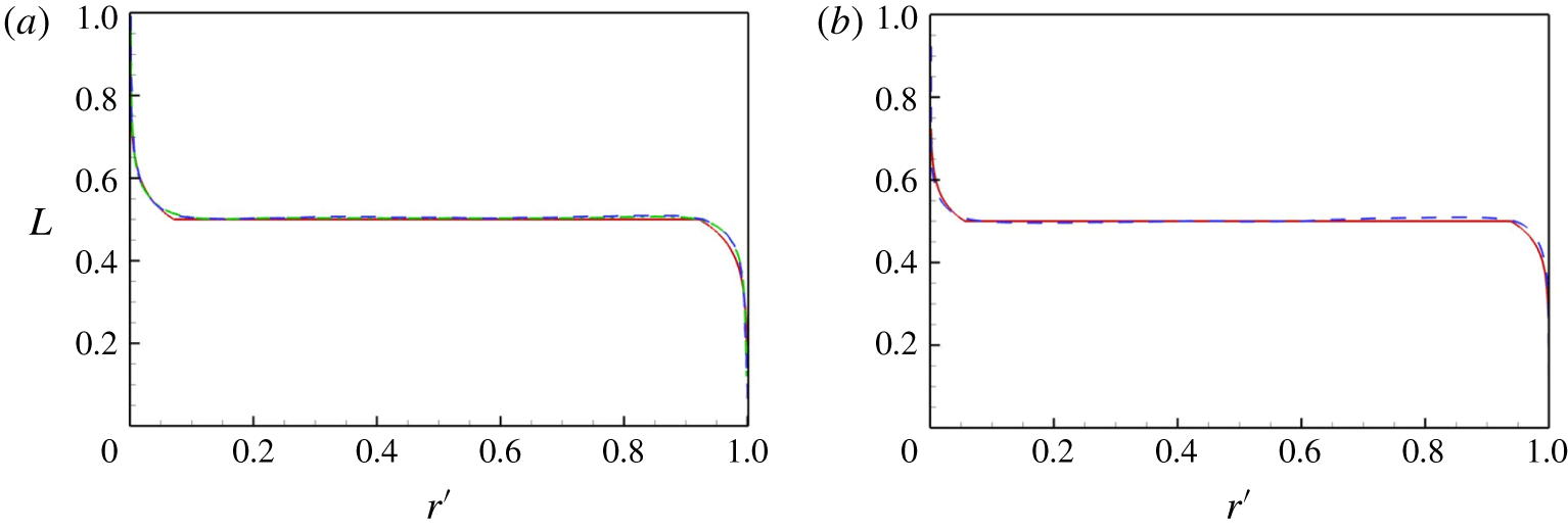
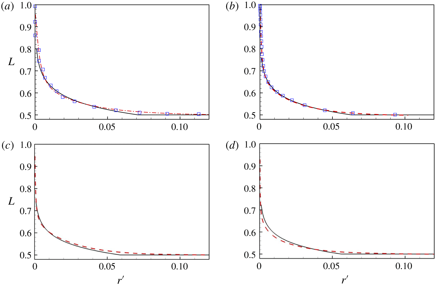
Radial angular momentum profiles. Model compared with DNS and LES. (a)  $Re_{i}=10^{5}$. (b)
 $Re_{i}=10^{6}$. ——, model prediction; - - - -, present LES; —⋅—, DNS by Ostilla-Mónico et al. (Reference Ostilla-Mónico, Verzicco, Grossmann and Lohse2016).

Radial angular momentum profiles. Model compared with DNS and LES. (a)  $Re_{i}=10^{5}$. (b)
 $Re_{i}=3\times 10^{5}$. (c)
 $Re_{i}=6\times 10^{5}$. (d)
 $Re_{i}=10^{6}$. ——, model prediction; - - - -, present LES; square symbols, DNS by Ostilla-Mónico et al. (Reference Ostilla-Mónico, Verzicco, Grossmann and Lohse2016).

4.4 Angular momentum profiles
It is straightforward to calculate profiles of the angular momentum  $L$ from the model. When normalized such that
 $L=rU_{\unicode[STIX]{x1D703}}/(\unicode[STIX]{x1D6FA}_{i}R_{i}^{2})$, this gives, with
 $r^{\prime }=(r-R_{i})/d$,
(I)  $L=(((1-\unicode[STIX]{x1D702})r^{\prime }/\unicode[STIX]{x1D702})+1)(1-(2Re_{\unicode[STIX]{x1D70F}_{i}}/Re_{i})((1/\unicode[STIX]{x1D705})\ln [2Re_{\unicode[STIX]{x1D70F}_{i}}r^{\prime }]+A)),0\leqslant r\leqslant \unicode[STIX]{x1D6FF}_{i}/d$,
(II)  $L=0.5,\unicode[STIX]{x1D6FF}_{i}/d\leqslant r^{\prime }\leqslant 1-\unicode[STIX]{x1D6FF}_{o}/d$,
(III)  $L=(((1-\unicode[STIX]{x1D702})r^{\prime }/\unicode[STIX]{x1D702})+1)(2\unicode[STIX]{x1D702}Re_{\unicode[STIX]{x1D70F}_{i}}/Re_{i})((1/\unicode[STIX]{x1D705})\ln [2\unicode[STIX]{x1D702}Re_{\unicode[STIX]{x1D70F}_{i}}(1-r^{\prime })]+A),1-\unicode[STIX]{x1D6FF}_{o}/d\leqslant r^{\prime }\leqslant 1$.
Figure 11 shows a comparison of the model and LES angular momentum profiles at  $Re_{i}=10^{5},10^{6}$, while figure 12 shows close-ups near the inner-cylinder walls for
 $Re_{i}=10^{5}$,
 $3\times 10^{5}$,
 $6\times 10^{5}$ and
 $10^{6}$. Comparisons between DNS (Ostilla-Mónico et al. Reference Ostilla-Mónico, Verzicco, Grossmann and Lohse2016), LES and the present model are satisfactory, except perhaps in the vicinity of the gradient discontinuity at the azimuthal velocity matching point. Since the wall-layer thickness decreases on outer scaling as
 $Re_{i}$ increases, the effect of the gradient discontinuity is more apparent as
 $Re_{i}$ increases. This could be addressed at the cost of an increase in model complexity.
4.5 Wall-layer thickness
Once the parameters  $Re_{\unicode[STIX]{x1D70F}_{i}}$ and
 $\unicode[STIX]{x1D6FF}_{i}$ have been determined, the velocity profile in the log region can be calculated. This allows calculations of the displacement and momentum thicknesses as functions of
 $Re_{\unicode[STIX]{x1D70F}_{i}}$. For the inner cylinder, these are defined presently as
 $$\begin{eqnarray}\unicode[STIX]{x1D6FF}^{\ast }=\int _{0}^{\unicode[STIX]{x1D6FF}_{i}}\left(1-\frac{\unicode[STIX]{x1D6FA}_{i}R_{i}-U_{\unicode[STIX]{x1D703}}}{U_{L}}\right)\text{d}r,\quad \unicode[STIX]{x1D703}=\int _{0}^{\unicode[STIX]{x1D6FF}_{i}}\frac{\unicode[STIX]{x1D6FA}_{i}R_{i}-U_{\unicode[STIX]{x1D703}}}{U_{L}}\left(1-\frac{\unicode[STIX]{x1D6FA}_{i}R_{i}-U_{\unicode[STIX]{x1D703}}}{U_{L}}\right)\text{d}r,\end{eqnarray}$$
where  $U_{L}=\unicode[STIX]{x1D6FA}_{i}R_{i}-\frac{1}{2}\unicode[STIX]{x1D6FA}_{i}R_{i}^{2}/(R_{i}+\unicode[STIX]{x1D6FF}_{i})$. Using the log part of the velocity profile in (4.1), these expressions can be evaluated analytically. The resulting expressions are shown in appendix C. Both
 $\unicode[STIX]{x1D6FF}^{\ast }$ and
 $\unicode[STIX]{x1D703}$ can be calculated from DNS and LES. An issue is the upper cutoff in the integrations. Presently, this was determined as
 $\unicode[STIX]{x1D6FF}_{99}=R_{i}-r$ where
 $r$ satisfies
 $$\begin{eqnarray}{\displaystyle \frac{(\unicode[STIX]{x1D6FA}_{i}R_{i}-U_{\unicode[STIX]{x1D703}})-(\unicode[STIX]{x1D6FA}_{i}R_{i}-0.5\unicode[STIX]{x1D6FA}_{i}R_{i}^{2}/r)}{(\unicode[STIX]{x1D6FA}_{i}R_{i}-0.5\unicode[STIX]{x1D6FA}_{i}R_{i}^{2}/r)}}<0.01.\end{eqnarray}$$
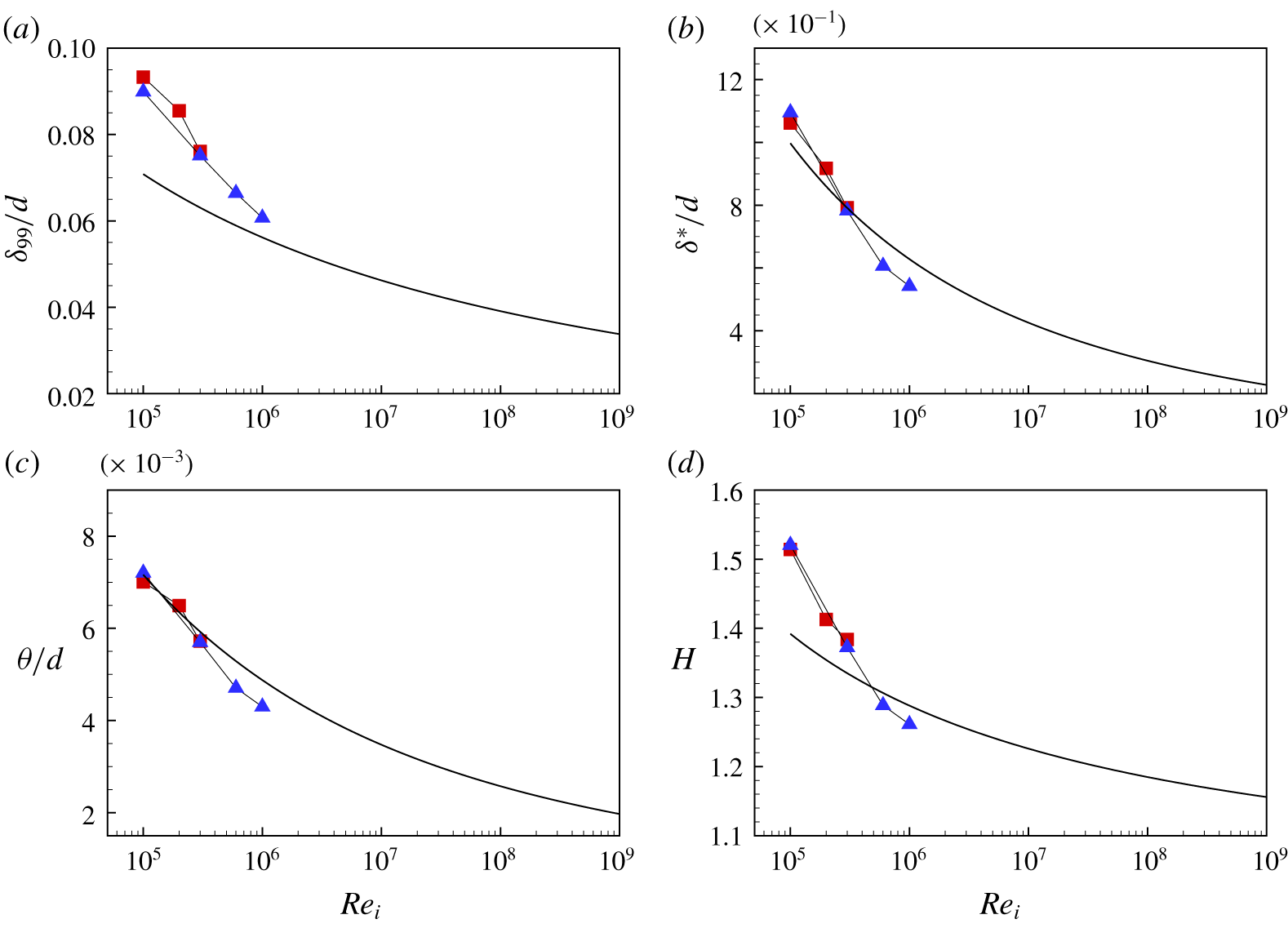
Results for  $\unicode[STIX]{x1D6FF}_{99},\unicode[STIX]{x1D6FF}^{\ast },\unicode[STIX]{x1D703}$ and the shape factor
 $H=\unicode[STIX]{x1D6FF}^{\ast }/\unicode[STIX]{x1D703}$ from the model are shown in figure 13 in comparison with both DNS and LES. Identifying
 $\unicode[STIX]{x1D6FF}_{i}$ with the measured
 $\unicode[STIX]{x1D6FF}_{99}$ provides an over-estimate. Both DNS and LES indicate a decline in the respective measures of wall-layer thicknesses as
 $Re_{i}$ increases, in agreement with the model.
Measures of boundary-layer thickness and shape factor  $H$ parameter versus
 $Re_{i}$. (a)
 $\unicode[STIX]{x1D6FF}_{99}/d$; (b)
 $\unicode[STIX]{x1D6FF}^{\ast }/d$; (c)
 $\unicode[STIX]{x1D703}/d$; (d)
 $H$. Solid line; present model. Symbols: ▪, DNS by Ostilla-Mónico et al. (Reference Ostilla-Mónico, Verzicco, Grossmann and Lohse2016); ▴ LES.

4.6 Discussion
The large  $Re_{i}$ limit of the model behaviour is of interest. It is clear that the model indicates that, when
 $Re_{i}(Ta)$ increases at fixed
 $\unicode[STIX]{x1D702}$ for smooth-wall flow on both cylinder surfaces,
 $\unicode[STIX]{x1D6FF}_{i}/d$ and
 $\unicode[STIX]{x1D6FF}_{o}/d$ (for the present outer wall profile) decline as the inverse of the Lambert
 $W$-function. This follows from (4.12) and (4.8). If the constant
 $L$ region separating the two wall layers remains intact at exceptionally large
 $Re_{i}$ or
 $Ta$, this suggests a limiting mean flow consisting of two asymptotically thinning wall layers in relation to the cylinder gap
 $d$, separated by a region where
 $$\begin{eqnarray}U_{\unicode[STIX]{x1D703}}={\displaystyle \frac{1}{2r}}(\unicode[STIX]{x1D6FA}_{i}R_{i}^{2}+\unicode[STIX]{x1D6FA}_{o}R_{o}^{2}).\end{eqnarray}$$
The present model does not contain a description of turbulent intensities, however, both DNS and LES appear to support the hypothesis that  $u_{\unicode[STIX]{x1D703}}^{\prime }u_{\unicode[STIX]{x1D703}}^{\prime }$ and other intensities scale as
 $u_{\unicode[STIX]{x1D70F}_{i}}^{2}$. An estimate can be made. Suppose that the peak azimuthal turbulence intensities are bounded by
 $(u_{\unicode[STIX]{x1D703}}^{\prime }u_{\unicode[STIX]{x1D703}}^{\prime })_{max}^{+}=A_{1}+B_{1}\ln (Re_{\unicode[STIX]{x1D70F}_{i}})$ (Lee & Moser Reference Lee and Moser2015) for absolute constants
 $A_{1},B_{1}$. Then
 $$\begin{eqnarray}\frac{(u_{\unicode[STIX]{x1D703}}^{\prime }u_{\unicode[STIX]{x1D703}}^{\prime })_{max}}{\unicode[STIX]{x1D6FA}_{i}^{2}R_{i}^{2}}\sim \frac{\left(A_{1}+B_{1}\ln (Re_{\unicode[STIX]{x1D70F}_{i}})\right)Re_{\unicode[STIX]{x1D70F}_{i}}^{2}}{Re_{i}^{2}}.\end{eqnarray}$$
For arbitrarily large  $Re_{i}$, (4.12) indicates that
 $Re_{\unicode[STIX]{x1D70F}_{i}}\sim Re_{i}/\text{ln}(Re_{i})$. It follows that, for a strictly smooth-wall flow,
 $(u_{\unicode[STIX]{x1D703}}^{\prime }u_{\unicode[STIX]{x1D703}}^{\prime })_{max}/(\unicode[STIX]{x1D6FA}_{i}^{2}R_{i}^{2})\sim \ln (Re_{\unicode[STIX]{x1D70F}_{i}})/(\ln (Re_{i}))^{2}$ when
 $Re_{i}\rightarrow \infty$. This shows slow but monotonic decrease to zero in this limit. Hence, the present results may be interpreted to imply that, for smooth-wall flow, the very large
 $Re_{i}$ state consists of a mean flow over most of the cylinder gap described by (4.21) together with slowly declining turbulent intensities in relation to the square of the driving cylinder surface speed
 $\unicode[STIX]{x1D6FA}_{i}R_{i}$. Huge
 $Re_{i}$ would be required to access this asymptotic state.
5 Rough walls
5.1 Roughness function
The extension of the present empirical model to turbulent, rough-wall flow with small-scale sandgrain-type roughness of scale  $k_{s}$ is now developed. For simplicity,
 $a=0$ is considered. The effects of sandgrain roughness is represented by use of a (Hama Reference Hama1954) roughness function
 $\unicode[STIX]{x0394}U^{+}(k_{s}^{+})$ where
 $k_{s}^{+}=k_{s}u_{\unicode[STIX]{x1D70F}_{i}}/\unicode[STIX]{x1D708}$. High Reynolds number pipe flow data for small-scale roughness (Shockling, Allen & Smits Reference Shockling, Allen and Smits2006) and recent DNS (Berghout et al. Reference Berghout, Zhu, Chung, Verzicco, Stevens and Lohse2019) at low Reynolds numbers both favour a Nikuradse-type (Nikuradse Reference Nikuradse1933) empirical correlation for
 $\unicode[STIX]{x0394}U^{+}(k_{s}^{+})$ in the transitional range of
 $k_{s}^{+}$. A generalized form of the (Colebrook Reference Colebrook1939) roughness function is utilized, given by
 $$\begin{eqnarray}\unicode[STIX]{x0394}^{+}U(k_{s}^{+})={\displaystyle \frac{1}{p\unicode[STIX]{x1D705}}}\ln (1+\unicode[STIX]{x1D6FD}(k_{s}^{+})^{p}),\quad \unicode[STIX]{x1D6FD}=\exp \left(p\unicode[STIX]{x1D705}(A-B)\right),\end{eqnarray}$$
where  $B$ is the Nikuradse constant and
 $p\geqslant 1$. The functional form for
 $\unicode[STIX]{x1D6FD}$ in (5.1) guarantees that, when
 $k_{s}$ is very large,
 $\unicode[STIX]{x0394}^{+}U(k_{s}^{+})\rightarrow 1/\unicode[STIX]{x1D705}\ln (k_{s}^{+})+A-B$ which is the large
 $k_{s}^{+}$, asymptotic Nikuradse form. The value
 $p=1$ corresponds to the Colebrook (Reference Colebrook1939) form. The limit
 $p\rightarrow \infty$ gives
 $\unicode[STIX]{x0394}^{+}U(k_{s}^{+})\rightarrow 0$ for
 $k_{s}^{+}<\exp [\unicode[STIX]{x1D705}(B-A)]$ and is equal to the Nikuradse limit form for
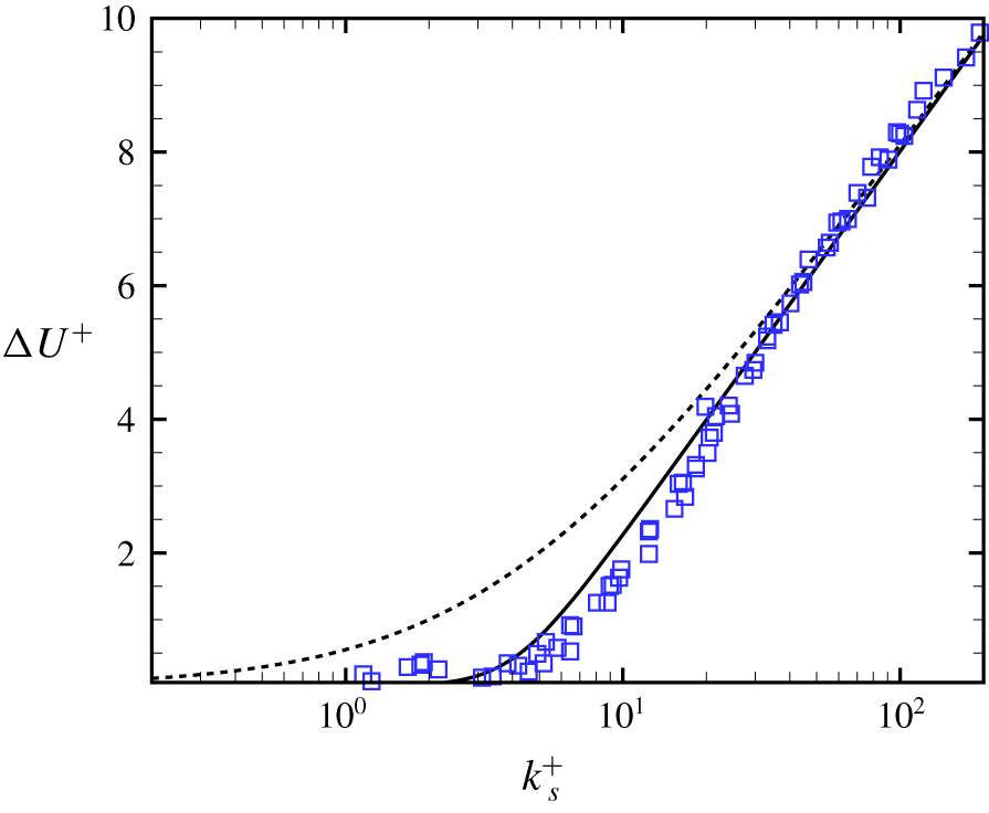
 $k_{s}^{+}>\exp [\unicode[STIX]{x1D705}(B-A)]$. Figure 14 shows equation (5.1) for
 $p=1$ (Colebrook) and
 $p=4$ with
 $\unicode[STIX]{x1D705}=0.4$,
 $A=4.5$,
 $B=8.0$ compared with the Nikuradse sandgrain data (Jiménez Reference Jiménez2004). Use of
 $p=4$, gives a substantially improved approximation to the data over
 $p=1$.
Value of  $\unicode[STIX]{x0394}U^{+}(k_{s}^{+})$ compared with the Nikuradse sandgrain data (Jiménez Reference Jiménez2004).
 $\unicode[STIX]{x1D705}=0.4$,
 $A=4.5$,
 $B=8.0$. Dashed line; (5.1),
 $p=1$. Solid line; (5.1),
 $p=4$.

5.2 Rough-wall empirical model
The inner wall can again be treated in isolation provided that the uniform angular momentum region exists, separating the wall layers on the inner- and outer-cylinder walls. For the inner wall, the velocity matching equation (4.5) is replaced by
 $$\begin{eqnarray}\unicode[STIX]{x1D6FA}_{i}R_{i}-u_{\unicode[STIX]{x1D70F}_{i}}\left(\frac{1}{\unicode[STIX]{x1D705}}\ln \left({\displaystyle \frac{\unicode[STIX]{x1D6FF}_{i}u_{\unicode[STIX]{x1D70F}_{i}}}{\unicode[STIX]{x1D708}}}\right)+A-\frac{1}{p\unicode[STIX]{x1D705}}\ln \left(1+\unicode[STIX]{x1D6FD}(k_{s}^{+})^{p}\right)\right)-{\displaystyle \frac{\unicode[STIX]{x1D6FA}_{i}R_{i}^{2}}{2(R_{i}+\unicode[STIX]{x1D6FF}_{i})}}=0.\end{eqnarray}$$
Equation (4.8) is retained. Again, a single equation for  $Re_{\unicode[STIX]{x1D70F}_{i}}$ can be obtained by substituting (4.8) into (5.2) with
 $\unicode[STIX]{x1D6FC}=1/2$, and converting to non-dimensional parameters to give
 $$\begin{eqnarray}-2ARe_{\unicode[STIX]{x1D70F}_{i}}+{\displaystyle \frac{Re_{i}(Re_{i}+Re_{\unicode[STIX]{x1D70F}_{i}})}{2Re_{i}+Re_{\unicode[STIX]{x1D70F}_{i}}}}-{\displaystyle \frac{2Re_{\unicode[STIX]{x1D70F}_{i}}}{p\unicode[STIX]{x1D705}}}\ln \left({\displaystyle \frac{(\unicode[STIX]{x1D702}Re_{\unicode[STIX]{x1D70F}_{i}}^{2})^{p}}{((1-\unicode[STIX]{x1D702})Re_{i})^{p}(1+\unicode[STIX]{x1D6FD}(2\unicode[STIX]{x1D716}Re_{\unicode[STIX]{x1D70F}_{i}})^{p})}}\right)=0,\end{eqnarray}$$
where  $\unicode[STIX]{x1D716}=k_{s}/d$ is the ratio of the sandgrain roughness scale to the cylinder gap. When
 $\unicode[STIX]{x1D716}=0$, equation (4.10) (with
 $a=0$) is recovered.
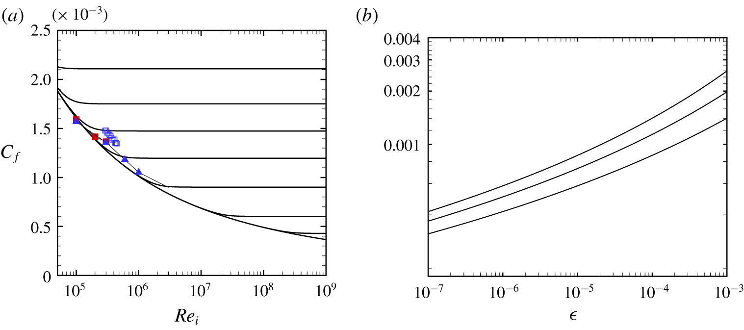
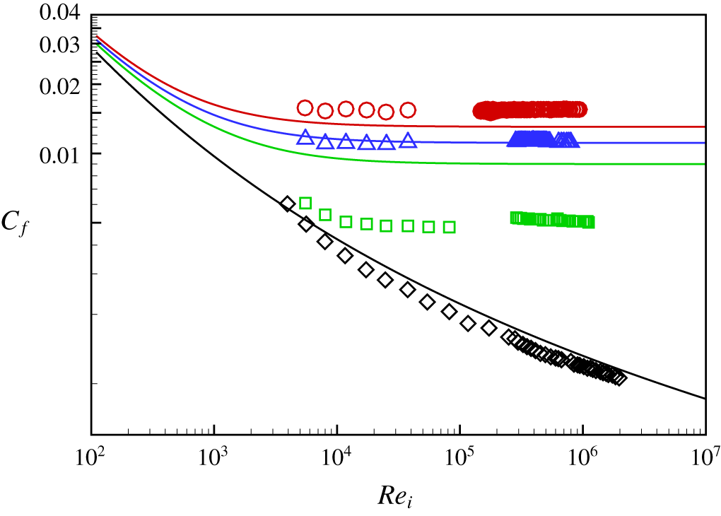
To illustrate the behaviour with rough walls, it is preferable to utilize the skin-friction coefficient defined as  $C_{f}\equiv 2\unicode[STIX]{x1D70F}_{i,w}/(\unicode[STIX]{x1D6FA}_{i}R_{i})^{2}$ where
 $\unicode[STIX]{x1D70F}_{i,w}=\unicode[STIX]{x1D70C}u_{\unicode[STIX]{x1D70F}_{i}}^{2}$. In terms of the other parameters
 $C_{f}$ can be expressed as
 $$\begin{eqnarray}C_{f}=8{\displaystyle \frac{Re_{\unicode[STIX]{x1D70F}_{i}}^{2}}{Re_{i}^{2}}}={\displaystyle \frac{4Nu}{\unicode[STIX]{x1D702}(1+\unicode[STIX]{x1D702})Re_{i}}}.\end{eqnarray}$$
Substituting an expression for  $Re_{\unicode[STIX]{x1D70F}_{i}}$ obtained from the first of (5.4) into (5.3) gives, after some algebra,
 $$\begin{eqnarray}\displaystyle & & \displaystyle 2-{\displaystyle \frac{8}{8+\sqrt{2}\sqrt{C_{f}}}}-\sqrt{2C_{f}}A\nonumber\\ \displaystyle & & \displaystyle \qquad -\,{\displaystyle \frac{\sqrt{2C_{f}}}{p\unicode[STIX]{x1D705}}}\ln \left({\displaystyle \frac{(\unicode[STIX]{x1D702}C_{f}Re_{i})^{p}}{(4(1-\unicode[STIX]{x1D702}))^{p}(2^{p}+(\sqrt{2C_{f}}\unicode[STIX]{x1D716}Re_{i})^{p}\exp (p\unicode[STIX]{x1D705}(A-B)))}}\right)=0.\end{eqnarray}$$
5.3 Fully rough-wall limit
Two limits are of interest. The first is the smooth-wall case  $\unicode[STIX]{x1D716}\rightarrow 0$ with
 $Re_{i}$ fixed. This follows directly by using
 $\unicode[STIX]{x1D716}=0$ in (5.5), The second is
 $Re_{i}\rightarrow \infty$ at any finite
 $\unicode[STIX]{x1D716}>0$, which takes the form
 $$\begin{eqnarray}2-{\displaystyle \frac{8}{8+\sqrt{2}\sqrt{C_{f}}}}-{\displaystyle \frac{\sqrt{2C_{f}}}{\unicode[STIX]{x1D705}}}\left(B\unicode[STIX]{x1D705}+\ln \left({\displaystyle \frac{\unicode[STIX]{x1D702}\sqrt{C_{f}}}{4\sqrt{2}\unicode[STIX]{x1D716}(1-\unicode[STIX]{x1D702})}}\right)\right)=0,\end{eqnarray}$$
which, as expected, is independent of  $p$. Hence, for fully rough-wall, turbulent wall-layer flow, the skin friction, and therefore the torque required to sustain the motion, becomes independent of
 $Re_{i}$, and depends only on
 $\unicode[STIX]{x1D702}$ and
 $\unicode[STIX]{x1D716}$.
Neither (5.5) nor (5.6) can be solved analytically for  $C_{f}$. But if the first two terms of the left-hand side of (5.6) are replaced by their leading-order Taylor expansion in the small quantity
 $\sqrt{C_{f}}$, then the result is
 $$\begin{eqnarray}1+{\displaystyle \frac{\sqrt{C_{f}}}{4\sqrt{2}}}-{\displaystyle \frac{\sqrt{2C_{f}}}{\unicode[STIX]{x1D705}}}\left(B\unicode[STIX]{x1D705}+\ln \left({\displaystyle \frac{\unicode[STIX]{x1D702}\sqrt{C_{f}}}{4\sqrt{2}\unicode[STIX]{x1D716}(1-\unicode[STIX]{x1D702})}}\right)\right)=0.\end{eqnarray}$$
This equation has the solution
 $$\begin{eqnarray}C_{f}={\displaystyle \frac{\unicode[STIX]{x1D705}^{2}}{2W^{2}(Z)}},\quad Z={\displaystyle \frac{\unicode[STIX]{x1D705}\unicode[STIX]{x1D702}\exp (B\unicode[STIX]{x1D705}-\unicode[STIX]{x1D705}/8)}{8\unicode[STIX]{x1D716}(1-\unicode[STIX]{x1D702})}}.\end{eqnarray}$$
For the range of parameters considered presently, numerical solutions to (5.5) agree with (5.8) to 3–4 significant figures. Other relevant quantities can now be calculated as
 $$\begin{eqnarray}k_{s}^{+}={\displaystyle \frac{1}{\sqrt{2}}}\unicode[STIX]{x1D716}\sqrt{C_{f}}Re_{i},\quad {\displaystyle \frac{\unicode[STIX]{x1D6FF}_{i}}{d}}={\displaystyle \frac{\unicode[STIX]{x1D702}\sqrt{C_{f}}}{4\sqrt{2}(1-\unicode[STIX]{x1D702})}}.\end{eqnarray}$$
Together with (5.7), the second of (5.9) shows that, when  $Re_{i}\rightarrow \infty$,
 $\unicode[STIX]{x1D6FF}_{i}/d$ is also independent of
 $Re_{i}$. The model predicts that, at sufficiently high
 $Re_{i}$ and sufficiently small
 $\unicode[STIX]{x1D716}$, the asymptotic rough-wall state consists of constant
 $C_{f}$ and wall-layer thickness
 $\unicode[STIX]{x1D6FF}_{i}/d$ that are independent of
 $Re_{i}$ (and hence of
 $Ta$). Figure 15(a) shows
 $C_{f}$ versus
 $Re_{i}$ with
 $\unicode[STIX]{x1D702}=0.909$ with several values of
 $\unicode[STIX]{x1D716}$ including the smooth-wall limit
 $\unicode[STIX]{x1D716}\rightarrow 0$, obtained from numerical solution of (5.5) with
 $p=4$,
 $\unicode[STIX]{x1D705}=0.4$,
 $A=4.5$,
 $B=8.0$. This is essentially a Moody (Reference Moody1944) diagram for a TC flow with a uniformly rough inner cylinder and an outer stationary cylinder, and with small-scale roughness. Figure 15(b) shows the fully rough
 $C_{f}(\unicode[STIX]{x1D702},\unicode[STIX]{x1D716})$ given by (5.8).
Skin-friction coefficient  $C_{f}$ for different roughness levels. (a)
 $C_{f}$ versus
 $Re_{i}$ for
 $\unicode[STIX]{x1D702}=0.909$. Solid lines: model prediction. Top to bottom
 $\unicode[STIX]{x1D716}=k_{s}/d=4\times 10^{-3},2\times 10^{-3},10^{-3},4\times 10^{-4},10^{-4},10^{-5},10^{-6},0$. ▪, DNS by Ostilla-Mónico et al. (Reference Ostilla-Mónico, Verzicco, Grossmann and Lohse2016); ▴, present LES. (b)
 $C_{f}$ versus
 $\unicode[STIX]{x1D716}=k_{s}/d$. Top to bottom
 $\unicode[STIX]{x1D702}=0.5,0.72,0.909$.

The large  $Re_{i}$ limit behaviour at finite
 $\unicode[STIX]{x1D716}$ is clear. For
 $\unicode[STIX]{x1D702}=0.909$, the second of (5.9) shows that
 $\unicode[STIX]{x1D6FF}_{i}/d=1.766\sqrt{C_{f}}$. Hence figure 15(a) with the ordinate rescaled also shows the large
 $Re_{i}$ behaviour of
 $\unicode[STIX]{x1D6FF}_{i}/d\sim \sqrt{C_{f}}$. For
 $\unicode[STIX]{x1D716}=10^{-3},10^{-4},10^{-5},10^{-6}$, the limiting values are
 $\unicode[STIX]{x1D6FF}_{i}/d=6.7\times 10^{-2},5.30\times 10^{-2},4.33\times 10^{-2},3.66\times 10^{-2}$ respectively. The model can be expected to be physically consistent provided that
 $\unicode[STIX]{x1D6FF}_{i}/k_{s}>10$ approximately, so that the log-like wall layer can exist. This is satisfied by all numerical solutions presented. In fact, a predictive estimate can be made of an upper bound on
 $\unicode[STIX]{x1D716}$ in order that
 $\unicode[STIX]{x1D6FF}_{i}/k_{s}\geqslant 10$. Using
 $\unicode[STIX]{x1D716}=(k_{s}/\unicode[STIX]{x1D6FF}_{i})\times (\unicode[STIX]{x1D6FF}_{i}/d)$ with
 $(k_{s}/\unicode[STIX]{x1D6FF}_{i})=1/10$ and using the second of (5.9) we can obtain
 $$\begin{eqnarray}10\unicode[STIX]{x1D716}_{b}={\displaystyle \frac{\unicode[STIX]{x1D702}\sqrt{C_{f}(\unicode[STIX]{x1D716}_{b})}}{4\sqrt{2}(1-\unicode[STIX]{x1D702})}}.\end{eqnarray}$$
Together with (5.8), it can be concluded that this bound  $\unicode[STIX]{x1D716}_{b}$ is a function of
 $\unicode[STIX]{x1D702}$ only. For
 $\unicode[STIX]{x1D702}=0.909,0.714,0.5$, solving (5.10) numerically gives
 $\unicode[STIX]{x1D716}_{b}=0.00884$,
 $0.00221$
 $0.000885$ respectively.
For completeness, the rough-wall model results in  $Nu,Ta$ variables are also shown. Using (5.4),
 $Nu$ is proportional to
 $Re_{i}$ with a coefficient proportional to
 $C_{f}$, and that depends on both
 $\unicode[STIX]{x1D702}$ and
 $\unicode[STIX]{x1D716}$. Using (3.3) and (5.4) we can obtain generally
 $$\begin{eqnarray}Nu={\displaystyle \frac{2\unicode[STIX]{x1D702}^{3}C_{f}}{(1+\unicode[STIX]{x1D702})^{2}}}Ta^{1/2}.\end{eqnarray}$$
Hence, in the fully rough limit, it follows that  $Nu\sim Ta^{1/2}$, again with a coefficient that depends on both
 $\unicode[STIX]{x1D702}$ and
 $\unicode[STIX]{x1D716}$. Figure 16 shows model results for
 $Nu$ versus
 $Ta$ for rough walls. The transition from smooth-wall flow where
 $Nu\sim Ta^{1/2}$ with Lambert function corrections to fully rough behaviour
 $Nu\sim Ta^{1/2}$ is clear.


Zhu et al. (Reference Zhu, Verschoof, Bakhuis, Huisman, Verzicco, Sun and Lohse2018) measures skin friction in TC flow with wall roughness consisting of 1–192 spanwise vertical rigs with square cross-section and with height ranging from 1.5 % to 10 % of the gap  $d$. Although these roughness heights are larger than the bound
 $\unicode[STIX]{x1D716}_{b}$ provided above, and are generally of the order of the present model estimate of the wall-layer thickness, and although the equivalent sandgrain roughness values are not known, a comparison between the present model and their data is nonetheless shown in figure 17. Here, the present
 $\unicode[STIX]{x1D716}=k_{s}/d$ is made equal to
 $h/d$, where
 $h$ is the rib height. The model calculation is reasonably close to experimental values for
 $h/d=0$,
 $0.075$ and
 $0.1$ but there are differences of order a factor of two for
 $h/d=0.05$. This is probably attributable to the reasons discussed above.
Comparison of roughness model (generalized Colebrook,  $p=4$), with data by Zhu et al. (Reference Zhu, Verschoof, Bakhuis, Huisman, Verzicco, Sun and Lohse2018). Model prediction: lines. From bottom to top:
 $\unicode[STIX]{x1D716}=h/d=0$,
 $0.05$,
 $0.075$ and
 $0.1$. Data by Zhu et al. (Reference Zhu, Verschoof, Bakhuis, Huisman, Verzicco, Sun and Lohse2018): ▫,
 $h/d=0$; ▫ (green),
 $h/d=0.05$; ▵,
 $h/d=0.075$; ○,
 $h/d=0.1$.

6 Conclusion
The present study uses wall-resolved large-eddy simulation to simulate Taylor–Couette flow with a narrow gap (radius ratio  $\unicode[STIX]{x1D702}=R_{i}/R_{o}=0.909$) between the inner, rotating cylinder and the outer stationary cylinder. The LES is implemented via a general curvilinear coordinate code with a non-staggered, velocity mesh. Fourth-order central difference schemes are used for all spatial discretization.
Two cases at  $Re_{i}=10^{5}$ and
 $3\times 10^{5}$ are used as verification cases. By comparing the mean-velocity profile
 $U^{+}$ and turbulent intensities
 $(u_{\unicode[STIX]{x1D703}}^{\prime }u_{\unicode[STIX]{x1D703}}^{\prime })^{+}$,
 $(u_{y}^{\prime }u_{y}^{\prime })^{+}$ and
 $(u_{r}^{\prime }u_{r}^{\prime })^{+}$, it is shown that the present LES framework can reasonably capture the main features of TC flows, including the quantitative behaviour of spanwise Taylor rolls, the log profile in the inner-cylinder mean-velocity profile and the angular momentum redistribution due to the presence of Taylor rolls, up to
 $Re_{i}=1\times 10^{6}$, which corresponds to a Taylor number
 $Ta=1.108\times 10^{12}$. Azimuthal turbulence intensities near the inner-cylinder wall indicate that the peak intensity scaled on the friction velocity increases though our full range of
 $Re_{i}$ while its location with respect to the inner wall surface, when scaled on inner variables, shows little variation.
A simple empirical model is developed that describes the mean-flow properties of Taylor–Couette flow when the outer cylinder is either stationary or co-rotating. The model consists of three contiguous flow regions; two contain turbulent wall layers, one at each cylinder wall, while the third is a central annular region of constant angular momentum. The model requires that this constant angular momentum per unit mass is known and equal to the average of angular momentum corresponding to rotation with inner- and outer-cylinder angular velocities  $\unicode[STIX]{x1D6FA}_{i},\unicode[STIX]{x1D6FA}_{o}$. It is supposed that this three-region state is produced by redistribution of angular momentum by either mean-flow or instantaneous fluctuating Taylor-roll motion, and further, that this persists to arbitrarily high Taylor number. Inside each wall layer, the flow is modelled by a standard log-like profile with
 $\unicode[STIX]{x1D705}=0.4,A=4.5$. The model takes an analytic form by implementing equality of azimuthal velocity at the region boundaries. It is closed by additional modelling of the thickness of the inner-cylinder wall layer as confined by a balance between radial turbulent diffusion and the wall-confinement effect of Taylor rolls. This gives the approximation that the inner wall-layer thickness is proportional to the local friction velocity divided by the cylinder angular velocity. A single arbitrary parameter is present which is set equal to
 $0.5$. The composite model is shown to postdict the effects of the cylinder ratio
 $\unicode[STIX]{x1D702}$, the Taylor number
 $Ta$ and the angular velocity ratio for co-rotation over the range of available DNS, experiment and the present LES. At large
 $Ta$, an approximate but sufficiently accurate model reduction gives a specific analytical form where the Nusselt number grows somewhat slower than the square root of the Taylor number. As
 $Ta$ increases, the wall layers shrink in thickness on the cylinder gap scale but grow on their respective inner scales.
A model extension to a rough inner wall comprising uniform sandgrain roughness is described in § 5. Use of a generalized Colebrook-type roughness function allows construction of a Moody diagram for Taylor–Couette flow. For given  $\unicode[STIX]{x1D702}$ and ratio of sandgrain roughness to cylinder gap, an asymptotic rough-wall state is found when
 $Re_{i}\rightarrow \infty$ with constant skin friction and wall-layer thickness that are both independent of
 $Re_{i}-Ta$ but that depend of the cylinder radii ratio
 $\unicode[STIX]{x1D702}$. Here, the Nusselt number is proportional to
 $Ta^{1/2}$.
At gigantic  $Re_{i}(Ta)$, for strictly smooth-wall flow, an asymptotic state is indicated where the uniform angular momentum region occupies almost all of the cylinder gap, with turbulence intensities that approach zero when
 $Re_{i}\rightarrow \infty$. This is consistent with some estimates of the infinite Reynolds number, smooth-wall limit for pipe flow (Pullin, Inoue & Saito Reference Pullin, Inoue and Saito2013; Cantwell Reference Cantwell2019). For any real cylinder surface, some small roughness level in relation to the cylinder gap dimension is expected. If this roughness is homogeneous, the roughness model extension predicts that the fully rough state will be the limit flow. This is a candidate for the ‘ultimate regime’ for Taylor–Couette flow discussed by Grossmann et al. (Reference Grossmann, Lohse and Sun2016). It is expected that the present roughness model can be used as a guide for the design of TC flow experiments with small-scale, homogeneous surface roughness.
Acknowledgements
This work was partially supported by the KAUST baseline research funds of R.S. The Cray XC40, Shaheen, at KAUST was utilized for all the reported LES. The authors gratefully acknowledge helpful comments from B. McKeon and N. Hutchins.
Declaration of interests
The authors report no conflict of interest.
Appendix A. Outer wall-layer thickness
Our aim here is to determine the outer wall-layer thickness given  $\unicode[STIX]{x1D6FF}_{o}$. Casting both (4.5)–(4.6) in non-dimensional form, and eliminating
 $Re_{i}$ in each equation using (4.8) gives, after some algebra,
 $$\begin{eqnarray}\displaystyle & \displaystyle \frac{a+\unicode[STIX]{x1D702}(2\tilde{\unicode[STIX]{x1D6FF}}_{i}(1-\unicode[STIX]{x1D702})+\unicode[STIX]{x1D702})}{2\tilde{\unicode[STIX]{x1D6FF}}_{i}(1-\unicode[STIX]{x1D702})(\tilde{\unicode[STIX]{x1D6FF}}_{i}(1-\unicode[STIX]{x1D702})+\unicode[STIX]{x1D702})}-4\left(\frac{1}{\unicode[STIX]{x1D705}}\log (2\tilde{\unicode[STIX]{x1D6FF}}_{i}Re_{\unicode[STIX]{x1D70F}_{i}})+A\right)=0, & \displaystyle\end{eqnarray}$$
 $$\begin{eqnarray}\displaystyle & \displaystyle \frac{a(1-2\tilde{\unicode[STIX]{x1D6FF}}_{o}(1-\unicode[STIX]{x1D702}))+\unicode[STIX]{x1D702}^{2}}{\tilde{\unicode[STIX]{x1D6FF}}_{i}(1-\tilde{\unicode[STIX]{x1D6FF}}_{o}(1-\unicode[STIX]{x1D702}))(1-\unicode[STIX]{x1D702})}-8\unicode[STIX]{x1D702}\left(\frac{1}{\unicode[STIX]{x1D705}}\log (2\tilde{\unicode[STIX]{x1D6FF}}_{o}\unicode[STIX]{x1D702}Re_{\unicode[STIX]{x1D70F}_{i}})+A\right)=0, & \displaystyle\end{eqnarray}$$
where  $\tilde{\unicode[STIX]{x1D6FF}}_{i}=\unicode[STIX]{x1D6FF}_{i}/d$ and
 $\tilde{\unicode[STIX]{x1D6FF}}_{o}=\unicode[STIX]{x1D6FF}_{o}/d$. Eliminating
 $\log (Re_{\unicode[STIX]{x1D70F}_{i}})$ from (A 1)–(A 2) gives a single equation linking
 $\tilde{\unicode[STIX]{x1D6FF}}_{o}$ and
 $\tilde{\unicode[STIX]{x1D6FF}}_{i}$
 $$\begin{eqnarray}\frac{\unicode[STIX]{x1D705}\left(\tilde{\unicode[STIX]{x1D6FF}}_{i}(1-2\tilde{\unicode[STIX]{x1D6FF}}_{o}(1-\unicode[STIX]{x1D702}))-\unicode[STIX]{x1D702}\tilde{\unicode[STIX]{x1D6FF}}_{o}\right)(\unicode[STIX]{x1D702}^{2}-a)}{\tilde{\unicode[STIX]{x1D6FF}}_{i}(1-\tilde{\unicode[STIX]{x1D6FF}}_{o}(1-\unicode[STIX]{x1D702}))(\tilde{\unicode[STIX]{x1D6FF}}_{i}(1-\unicode[STIX]{x1D702})+\unicode[STIX]{x1D702})}-8\unicode[STIX]{x1D702}\log \left(\frac{\tilde{\unicode[STIX]{x1D6FF}}_{i}}{\unicode[STIX]{x1D702}\tilde{\unicode[STIX]{x1D6FF}}_{o}}\right)=0.\end{eqnarray}$$
For the present application it is expected that both  $\tilde{\unicode[STIX]{x1D6FF}}_{i}$,
 $\tilde{\unicode[STIX]{x1D6FF}}_{o}$ are rather smaller than unity. This suggests the expansion
 $\tilde{\unicode[STIX]{x1D6FF}}_{o}=\unicode[STIX]{x1D700}\tilde{\unicode[STIX]{x1D6FF}}_{i}^{(1)}+\unicode[STIX]{x1D700}^{2}\tilde{\unicode[STIX]{x1D6FF}}_{i}^{(2)}+\unicode[STIX]{x1D700}^{3}\tilde{\unicode[STIX]{x1D6FF}}_{i}^{(3)}+\cdots$ where
 $\unicode[STIX]{x1D700}$ is a nominally small parameter. Next, substitute into (A 3) and Taylor expand in
 $\unicode[STIX]{x1D700}$ about
 $\unicode[STIX]{x1D700}=0$. Equating the coefficients of ascending powers of
 $\unicode[STIX]{x1D700}$ to zero gives a sequence of equations for
 $\tilde{\unicode[STIX]{x1D6FF}}_{o}^{(n)},n=1,2\ldots$ . These can be solved sequentially. To the third order it is then found that
 $$\begin{eqnarray}\displaystyle \tilde{\unicode[STIX]{x1D6FF}}_{0} & = & \displaystyle \frac{1}{\unicode[STIX]{x1D702}}\tilde{\unicode[STIX]{x1D6FF}}_{i}+\frac{2\unicode[STIX]{x1D705}(1-\unicode[STIX]{x1D702})(\unicode[STIX]{x1D702}^{2}-a)}{\unicode[STIX]{x1D702}^{4}(8-\unicode[STIX]{x1D705})+\unicode[STIX]{x1D705}a\unicode[STIX]{x1D702}^{2}}\tilde{\unicode[STIX]{x1D6FF}}_{i}^{2}\nonumber\\ \displaystyle & & \displaystyle +\,\frac{4\unicode[STIX]{x1D705}^{2}(1-\unicode[STIX]{x1D702})^{2}(\unicode[STIX]{x1D702}^{2}-a)^{2}(\unicode[STIX]{x1D702}^{2}(12-\unicode[STIX]{x1D705})+a\unicode[STIX]{x1D705})}{(\unicode[STIX]{x1D702}^{3}(8-\unicode[STIX]{x1D705})+a\unicode[STIX]{x1D702}\unicode[STIX]{x1D705})^{3}}\tilde{\unicode[STIX]{x1D6FF}}_{i}^{3}+\cdots \,.\end{eqnarray}$$
For the cases considered presently, the leading order on the right-hand side of (A 4) agrees to two, and generally to three, significant digits with numerical solutions to (A 3). As an example take  $Re_{i}=10^{6}$,
 $\unicode[STIX]{x1D702}=0.909$,
 $a=0$ for which we find
 $\tilde{\unicode[STIX]{x1D6FF}}_{i}=0.0589$. Numerical solution of (A 3) gives
 $\tilde{\unicode[STIX]{x1D6FF}}_{o}=0.064836737\!\ldots$ . Truncating (A 4) at the first, second and third terms respectively gives the sequence
 $\tilde{\unicode[STIX]{x1D6FF}}_{o}=0.064796479\!\ldots \!,0.064836698\!\ldots \!,0.064836736\!\ldots$ respectively. Perhaps interestingly, the leading-order approximation
 $\tilde{\unicode[STIX]{x1D6FF}}_{0}=\tilde{\unicode[STIX]{x1D6FF}}_{i}/\unicode[STIX]{x1D702}$, when combined with (4.4), shows that
 $\unicode[STIX]{x1D6FF}_{o}^{+}=\unicode[STIX]{x1D6FF}_{i}^{+}$: relative to their own local skin-friction conditions, both wall layers are of equal extent in their respective inner scalings.
Appendix B. Small gap limit $\unicode[STIX]{x1D702}\rightarrow 1$

When  $\unicode[STIX]{x1D702}\rightarrow 1$ at fixed
 $Ta$, the three-region model reaches a limit because the extent of the central constant angular momentum region reduces to zero. In other words, the two log layers occupy the whole gap. For values of
 $\unicode[STIX]{x1D702}$ greater than this limiting value, a more physically appropriate model would be two log layers that meet at the gap centre (Grossmann & Lohse Reference Grossmann and Lohse2011). Brief details are given where again we take
 $a=0$. The two wall-layer profiles (4.1) and (4.3) are assumed to be equal at the gap centre
 $r=R_{i}+d/2$. Following the analysis of § 4, a single equation for
 $Re_{\unicode[STIX]{x1D70F}_{i}}$ can be developed as
 $$\begin{eqnarray}Re_{i}-2A(1+\unicode[STIX]{x1D702})Re_{\unicode[STIX]{x1D70F}_{i}}-\frac{2Re_{\unicode[STIX]{x1D70F}_{i}}}{\unicode[STIX]{x1D705}}\left[(1+\unicode[STIX]{x1D702})\ln Re_{\unicode[STIX]{x1D70F}_{i}}+\unicode[STIX]{x1D702}\ln \unicode[STIX]{x1D702}\right]=0.\end{eqnarray}$$
No closure equation is required. This equation has an analytic solution. When expressed in terms of  $(Nu,Ta)$, this is
 $$\begin{eqnarray}Nu(Ta,\unicode[STIX]{x1D702},a)=\frac{4\unicode[STIX]{x1D705}^{2}\unicode[STIX]{x1D702}^{3}Ta^{1/2}}{(1+\unicode[STIX]{x1D702})^{4}(W(Z_{3}))^{2}},\quad Z_{3}=\frac{4\unicode[STIX]{x1D705}\unicode[STIX]{x1D702}^{2+\unicode[STIX]{x1D702}/(1+\unicode[STIX]{x1D702})}Ta^{1/2}\exp [\unicode[STIX]{x1D705}A]}{(1+\unicode[STIX]{x1D702})^{4}}.\end{eqnarray}$$
Figure 18 shows (B 2) compared with (4.15) for  $Ta=10^{12}$. The curves intersect at
 $\unicode[STIX]{x1D702}=0.99134$, which is close to the value
 $\unicode[STIX]{x1D702}=0.99084$ where
 $\unicode[STIX]{x1D6FF}_{i}+\unicode[STIX]{x1D6FF}_{o}=d$ for the present three-region model. These are not identical because, at the latter value, the three-region model still contains one point (gap centre) where the angular momentum corresponds to the constraint, whereas this plays no role in the two-region model. The above suggests a transition from a three-region structure for values of
 $\unicode[STIX]{x1D702}$ less than that at the intersection point, to a two-region structure that is close to plane-Couette flow for greater values. It is noted that the two-region model gives a poor approximation to the LES estimate of
 $Nu$ at
 $\unicode[STIX]{x1D702}=0.909$.
Value of  $Nu$ versus
 $\unicode[STIX]{x1D702}$,
 $a=0$.
 $Ta=10^{12}$. Dashed line; two-region model, (B 2). Solid line; present three-region model. Filled triangle; LES.

Appendix C. Expressions for $\unicode[STIX]{x1D6FF}^{\ast },\unicode[STIX]{x1D6FF}_{\unicode[STIX]{x1D703}}$

Here expressions for  $\unicode[STIX]{x1D6FF}^{\ast }/d$ and
 $\unicode[STIX]{x1D6FF}_{\unicode[STIX]{x1D703}}/d$ are provided. These are dimensionless forms of the integral definitions given in (4.19)
 $$\begin{eqnarray}\frac{\unicode[STIX]{x1D6FF}^{\ast }}{d}=\tilde{\unicode[STIX]{x1D6FF}}_{i}-{\displaystyle \frac{4(\tilde{\unicode[STIX]{x1D6FF}}_{i}(1-\unicode[STIX]{x1D702})+\unicode[STIX]{x1D702})((\unicode[STIX]{x1D705}A-1)Re_{\unicode[STIX]{x1D70F}_{i}}+\log (2\tilde{\unicode[STIX]{x1D6FF}}_{i}Re_{\unicode[STIX]{x1D70F}_{i}}))}{G}},\end{eqnarray}$$
 $$\begin{eqnarray}\displaystyle \frac{\unicode[STIX]{x1D6FF}_{\unicode[STIX]{x1D703}}}{d} & = & \displaystyle -\left(4\right.\tilde{\unicode[STIX]{x1D6FF}}_{i}QRe_{\unicode[STIX]{x1D70F}_{i}}\left(4\right.(2+\unicode[STIX]{x1D705}A(\unicode[STIX]{x1D705}A-2))QRe_{\unicode[STIX]{x1D70F}_{i}}-\unicode[STIX]{x1D705}(\unicode[STIX]{x1D705}A-1)Re_{i}S+\log [2\tilde{\unicode[STIX]{x1D6FF}}_{i}Re_{\unicode[STIX]{x1D70F}_{i}}]\nonumber\\ \displaystyle & & \displaystyle \times \,(8(\unicode[STIX]{x1D705}A-1)QRe_{\unicode[STIX]{x1D70F}_{i}}-\unicode[STIX]{x1D705}Re_{i}S+4Q\log [2\tilde{\unicode[STIX]{x1D6FF}}_{i}Re_{\unicode[STIX]{x1D70F}_{i}}])\!\!\left.\right)\!\!\left.\right)\!/G^{2},\end{eqnarray}$$
where  $\tilde{\unicode[STIX]{x1D6FF}}_{i}=\unicode[STIX]{x1D6FF}_{i}/d$, and
 $$\begin{eqnarray}S=2\tilde{\unicode[STIX]{x1D6FF}}_{i}(1-\unicode[STIX]{x1D702})+\unicode[STIX]{x1D702},\quad Q=\tilde{\unicode[STIX]{x1D6FF}}_{i}(1-\unicode[STIX]{x1D702})+\unicode[STIX]{x1D702},\quad G=\unicode[STIX]{x1D705}Re_{i}S.\end{eqnarray}$$