1 Introduction
The entity relation detection (ERD) task aims at finding relationships between pairs of named entities (NEs) in text. NEs such as persons may be related to organization entities via organization affiliation relation (‘John is the founder of Xyz Corp.’). Organization entities may be related to location entities via physical location relation (‘Xyz Corp is located in North Carolina’) and persons may be related to one another via social relations (‘John and Mary were married last year’).
Availability of annotated corpora (Doddington et al. Reference Doddington, Mitchell, Przybocki, Ramshaw, Strassel and Weischedel2004) and introduction of shared tasks (e.g., Carreras and Màrquez Reference Carreras and Màrquez2005; Farkas et al. Reference Farkas, Vincze, Móra, Csirik and Szarvas2010) have spurred a large amount of research in this field in recent times. Researchers have used supervised and semi-supervised approaches (Hasegawa, Sekine and Grishman Reference Hasegawa, Sekine and Grishman2004; Jiang Reference Jiang2009; Mintz et al. Reference Mintz, Bills, Snow and Jurafsky2009), and explored rich features (Kambhatla Reference Kambhatla2004),, kernel design (Culotta and Sorensen Reference Culotta and Sorensen2004; Bunescu and Mooney Reference Bunescu and Mooney2005; Zhou et al. Reference Zhou, Jian, Jie and Min2005; Qian et al. Reference Qian, Zhou, Kong, Zhu and Qian2008), and joint inference (Chan and Roth Reference Chan and Roth2011), to detect predefined relations between NEs.
In this work, we explore how the latent semantics of the text can help in detecting entity relations. Specifically, we are interested in the underlying topic distributions. Intuitively, topics such as marriage or birth could be indicative of a social relationship between the participating entities. Similarly, topics such as nationality or recruitment could be indicative of an affiliation relation between the participating entities. Thus in this paper, we investigate if hidden topic distributions indicative of entity relations can be effectively learned.
In order to achieve this, we adapt the Latent Dirichlet Allocation (LDA) approach to solve the ERD task. There are a number of challenges in employing the LDA framework for ERD. Primarily, the basic LDA model is unsupervised, and hence the discovered topics may not help classification. This problem has been solved in supervised models such as labeled LDA (LLDA) (Ramage et al. Reference Ramage, Hall, Nallapati and Manning2009) and supervised LDA (sLDA) (Blei and McAuliffe Reference Blei and McAuliffe2008). While LLDA and sLDA are powerful generative models that capture the underlying semantics of texts pertinent to classes of interest, we found during our preliminary experiments that they have trouble discovering marginal classes in ERD and do not naturally incorporate rich feature sets.
In order to incorporate the capabilities desirable for relation detection, we build our ERD system, ERD-MedLDA, based on Maximum Entropy Discriminant Latent Dirichlet Allocation (MedLDA) from Zhu, Ahmed and Xing (Reference Zhu, Ahmed and Xing2009). MedLDA is a supervised extension of LDA that combines the capability of capturing latent semantics with maximum margin learning. Specifically, MedLDA is a combination of sLDA and support vector machines (SVMs); thus, it integrates maximum likelihood estimation (MLE) and maximum margin estimation (MME). Further, in order to employ rich and heterogeneous features we introduce a separate exponential family distribution for each feature, similar to Shan, Banerjee and Oza (Reference Shan, Banerjee and Oza2009), into our ERD-MedLDA model.
The relation detection task is formulated within the topic model framework in ERD-MedLDA as follows. Occurrences of pairs of NE mentionsFootnote 1 in a document and the text between them is considered as a mini-document. Each mini-document has a relation type (analogous to the response variable in a supervised topic model). The supervised topic model discovers a latent topic representation of the mini-documents and a response parameter distribution. The topic representation is discovered with observed response variables during training, which influences topic discovery towards the response variables. During prediction, the topic distribution of each mini-document can form a prediction of the relation types.
We carry out experiments to measure the effectiveness of our approach and compare it to SVM-based and LLDA-based models, as well as to a previous work using the same corpus. We also analyze the discovered topics and measure the effectiveness of incorporating different features in our model relative to other models. Our approach exhibits better overall precision, recall, and F-measure than baseline systems. We also find that ERD-MedLDA shows consistent capability for incorporation and improvement due to a variety of heterogeneous features.
The rest of the paper is organized as follows. We describe the proposed model in Section 2, and Section 3 describes the data and the task formulation. The features that we incorporate are explained in Section 4. Section 5 presents the experiments and Section 6 presents analyses. We discuss the related work in Section 7 before concluding in Section 8.
2 ERD-MedLDA
ERD-MedLDA is based on the principle of hierarchical Bayesian models. The basic LDA is an unsupervised model and the resulting topics may not help with classification tasks. However, with the explicit addition of supervised information (such as response variables), the resulting topic models have good predictive power for classification and regression. MedLDA model from Zhu et al. (Reference Zhu, Ahmed and Xing2009) is one such extension of LDA, where the class information is added to the model. Further, MedLDA integrates maximum margin learning and topic models by optimizing a single objective function with a set of expected margin constraints.
In this section, we explain the development of ERD-MedLDA as follows: We first explain the MedLDA model from Zhu et al. (Reference Zhu, Ahmed and Xing2009) and our modifications to it in Section 2.1. Section 2.2 describes further modifications that allow for the incorporation of heterogeneous features, Section 2.3 describes inference and estimation procedures, and, finally, Section 2.4 describes how relation detection is performed under the model.
The following notation is used in this paper:
K – The total number of topics
N – The total number of words and features in a document
C – The total number of relation types
α1:K – K-dimensional parameter of a Dirichlet distribution
β1:K – Parameters for K component distribution over the words
θ1:K – K-dimensional parameters of topic distribution variables over a
– document
η1:C – Parameters for C component distribution over the relation types
z d1:dN – Variables representing a sequence of topics in a specific document, d
w d1:dN – A finite set of observed variables that represent a specific document, d
y 1:C – A finite set of observed variables which represents relation types
D – A collection of documents denoted by D = w1, w2, . . ., wD
For brevity, we use bold case symbols for vectors and drop the subscript where dimensionality is unambiguous.
2.1 MedLDA
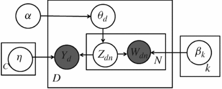
The MedLDA model described in Zhu et al. (Reference Zhu, Ahmed and Xing2009) is illustrated in Figure 1. Here, θ is a K-dimensional topic distribution variable, which is sampled from a Dirichlet distribution Dirichlet(α). Like common LDAs, MedLDA uses independence assumption for a finite set of random variables Z 1, . . ., Zn which are independent and identically distributed, conditioned on the parameter, θ. Like its predecessor, sLDA, MedLDA is a supervised model. A response variable Y connected to each document is added for incorporating supervised side information. The supervised side information is expected to make MedLDA topic discoveries more useful for classification tasks. Zhu, Ahmed and Xing's (Reference Zhu, Ahmed and Xing2009) MedLDA model can be used in both regression and classification. Concretely, Y is drawn from η1:C, a C × K-dimensional vector and the topic distribution z 1:N. Note that the plate diagram for MedLDA is quite similar to sLDA (Blei and McAuliffe Reference Blei and McAuliffe2008). But there is a difference – sLDA focuses on building regression models, and thus the response variable Y in sLDA is generated by a normal distribution. In regression, similar to sLDA, a normal distribution is used for generating Y, while in classification, MedLDA uses the maximum-margin principle to directly generate Y.
MedLDA.
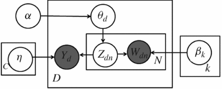
Based on the plate diagram, the joint distribution of latent and observable variables for our MedLDA-based relation detection is given by:

Another important difference from sLDA lies in the fact that MedLDA does joint learning with both MME and MLE. The joint learning for classification is done in two stages, unsupervised topic discovery and multi-class classification. During training, EM algorithms are utilized to infer the posterior distribution of the hidden variables θ, z, and η. During testing, the trained models are used to predict relation types y.
2.2 Fine mixed-membership MedLDA
MedLDA is already a mixed-membership model and although the MedLDA model described above can be applied to detection and classification tasks, we felt a few modifications were necessary before it can be effective in predicting relation types. In particular, MedLDA is designed for using a homogeneous component distribution and we required it to use heterogeneous features.
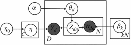
As we can see from the plate model in Figure 1, each of w 1:N is assumed to be generated from one of the discrete component distributions. In each document, bag of words are the same type of objects. The set of distributions remain the same across all words. Thus the original MedLDA is designed to handle data points with homogeneous features such as words. But previous work in relation detection has shown that it is important to incorporate part-of-speech tags, NEs, grammatical dependencies, and other linguistic features. We achieve this by introducing a separate exponential family distribution for each feature similar to (Shan et al. Reference Shan, Banerjee and Oza2009). Thus, our relation detection model is really a mixed-member Bayesian network. Figure 2 illustrates our model with this extension.
Fine mixed-membership MedLDA.
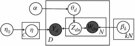
Figure 2 is very similar to Figure 1. There are two differences: First, the topic component number k is now kN and second, there is another component η0 before the response parameter η. We made the first modification in order to incorporate heterogeneous features. Note that now we have βdni rather than only βdi since we have drawn separate distributions for each word (or feature) n.
In MedLDA, Zhu et al. (Reference Zhu, Ahmed and Xing2009) have in fact introduced the idea that η is sampled from a prior p 0(η). We too follow the same idea and show it as a hyper-parameter in Figure 2 for clarity. Like MedLDA, we assume that there are C classes and K topics. In our work, C is the number of relation types. However, unlike MedLDA, the response parameter η1:C in our model is a matrix with C × K-dimensional softmax parameters as rows.
The generative process for each document in this model is similar to that given in (Shan et al. Reference Shan, Banerjee and Oza2009) and is as follows:
(1) Sample a component proportion θd ~ Dirichlet(α),
(2) For each feature like word, part-of-speech, NE in the document,
(a) For n ∈ {1, \ldots, N}, sample zdn = i ~ Discrete(θd)
(b) For n ∈ {1, \ldots, N}, sample wdn ~ P(wdn|βdni, zdn)
(3) Sample the relation type label for a document from a softmax distribution, two steps are involved,
(a) For j ∈ {1, \ldots, C}, sample ηj ~ Norm(0, η0)
(b) For j ∈ {1, \ldots, C}, yd ~ softmax


In step 2, index i is the number of the topic component which ranges from 1 : K. P(wdn|βdni, zdn) in 2(b) is an exponential family distribution.
Like the original MedLDA, we make use of a prior p 0(η) where p 0 = N(0,I) to sample the response parameter η. That is, η is taken as a variable rather than a hyper-parameter like α and β. η0 is the hyper-parameter for η and it is sampled C times. Namely, for each relation type, a vector of response parameters will be sampled and they will in turn be used to sample relation types.
For the sampling in step 3(b), a softmax distribution is employed. Softmax is a variation of logistic regression. Logistic regression is usually used for binary classification while softmax is for multi-class classification. Softmax is a mature statistical method for classifications, easy to compute, and is appropriate for handling missing features. The input for the softmax distribution is z, namely, the mean of z for all words/features.
Note that we do not directly use maximum margin principle for classification. This is another modification we make in the model. The original MedLDA's model for classification comprises of two separate parts – the first part is an unsupervised LDA that does MLE for modeling topics and the second part is an SVM that does MME for classification. Zhu, Ahmed and Xing's motivation of doing so is that calculations of partition factors or normalization factors are too hard and too slow. However, we believe that this separation cannot make full use of the advantages of the integration of MME and MLE. In the learning process, topic discoveries biased by supervised side information should be more helpful than topics discovered or learned in unsupervised fashion. Though the learning of normalization factor for classification will be slower, it is not intractable, and speed-ups can be achieved by selecting suitable sampling methods and by good optimizations and approximations.
Thus, a joint distribution can be written as:

The second term is the same as that defined in (1). The first term, the prior distribution of η, is defined as a normal distribution.
The density function for w, y, after θ and z are integrated out, is given by:

Since relation detection only involves token features (even though these features are heterogeneous in nature, ranging from bag of words, parts-of-speech, chunk types, and so on), they are discrete symbols. Hence, before we find continuous features, such as numerical values, all features have discrete distributions.
With this extension, the distribution for generating wdn not only depends on zdn, but also on what kind of features are employed. Therefore, by choosing an appropriate exponential family distribution for each feature (in our relation detection, all features involve discrete distributions with diverse parameters), our ERD-MedLDA model can integrate diverse features of different types or the same features with different parameters.
2.3 Inference and estimation
In (Zhu et al. Reference Zhu, Ahmed and Xing2009), MedLDA integrates a Bayesian sLDA and a SVM for both MLE and MME. In our work, we follow the same overall approach. However, as shown in our generative process, instead of only using unsupervised LDA for topic modeling, we use fully supervised MedLDA for both topic modeling and the final classification. Yet, the inference is slower because of the normalization factor in the probability distribution of Y and also because we draw different distributions for each word. To remedy this, we make use of a strategy similar to Shan et al. (Reference Shan, Banerjee and Oza2009). Namely, for features of the same type, we sample them with the same exponential distributions using parameters averaged from the training data, which makes the learning much faster and efficient.
In our model, the learning task is to obtain an optimal set of parameters α, β and p(η) such that the likelihood of observing the whole feature set and the relation types, p(w, y|α, β, p(η)), are maximized. However, the calculation of the likelihood function (3) is intractable. Following the generative process, parameter estimation and inferences can be made with either Gibbs sampling or EM-based variational methods. We use variational methods since we adapt MedLDA packageFootnote 2 to mixed-membership ERD-MedLDA and train relation detection models.
Specifically, to obtain a tractable lower bound, we consider an entire family of parameterized lower bounds with a set of free variational parameters, and pick the best lower bounds by optimizing the lower bound with respect to the free variational parameters.
2.3.1 Variational inference
The EM-based variational method involves an E-step and a M-step. In the E-step, the latent variable distributions are computed while in the M-step, parameter estimation is done by maximizing the expectation of the complete likelihood distribution. As we know, in order to use MedLDA to make predictions on the relation types, the key inferential problem that we need to solve is that of computing the posterior distribution of the hidden variables given a document,

where, the denominator is (3), which is the probability of observed variables given all parameters; and the numerator is the probability of all observed variables plus sampled parameters given hyper-parameter for one document.
The partition function obtained from (3) and (4) is intractable; thus, it cannot be computed in closed form. Hence, the same approximation as in Zhu et al. (Reference Zhu, Ahmed and Xing2009) is made. The upper bound (formalized as Lbs(q)) of the negative log-likelihood -log p(w, y|α, β, η) – is given as,

where Ls refers to the likelihood function of sLDA and  is the Kullback-Leibler (KL) divergence;
 is the expected value and
 is the entropy.
Equation (5) can be expanded as follows (please refer to the Appendix A for details).

Then, with exactly the same idea of integration of MLE and MME as in Zhu et al (Reference Zhu, Ahmed and Xing2009), we can define the integrated training of ERD-MedLDA as a constrained optimization problem in (7).
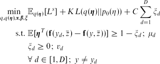
where μ, v are Lagrange multipliers, ξ is the slack variable tolerating errors in training data. yd is the true label while y is the prediction. So, f(yd, zd) − f(y,zd) is the difference between truth and prediction, which we call expected margin. Namely, the former is the average boundary composed of true labels and the latter is the average boundary of predicted labels. The smaller the difference, the closer it is to the true labels. This is essentially the advantage of ERD-MedLDA over other MLE or maximum-entropy models. Further, since ERD-MedLDA also employs regular MLE for data generated from sampling, it enjoys advantages of both kinds of learning. That is, it takes care of sufficient statistics as well as handles examples that are around the decision boundary with support vectors. When Lagrange multipliers are not zeros, terms related to them act as a regularizer, biasing the model towards discovering a latent representation. Thus, more accurate predictions will be obtained on difficult examples located at decision boundaries. These latent representations are fixed for words in a document and therefore yield better discriminant power.
Then, the Lagrangian  of (7) is similar to the one for classification as in (Zhu et al. Reference Zhu, Ahmed and Xing2009) except that the first term is supervised rather than unsupervised. This equation is reproduced below for readability.
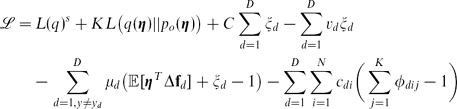
where  and the last term is from the normalization condition
 .
2.3.2 Parameter estimation
In the last section, we constructed variational parameters for approximating hidden variables θ, z, and η. Following this, the EM algorithm will iteratively solve the approximation problem with two steps:
(1) E-step: infer the posterior distribution of the hidden variables θ, z, and η, where, for θ and z, inferring the posterior distributions are in fact to fit the variational parameters φ and γ; while for η, more complex issues will be involved.
(2) M-step: estimate the unknown model parameters α, β.
The update rules are in fact done by sequentially taking partial derivative of (8) over related variables. We optimize the Lagrangian over each of the related variables in the following order γ, φ, q(η), α, and β. Since the constraints in (8) are not on θ (its variational γ), α, or β, the update rules are the same as LDA or sLDA.
The update of φ is the same as MedLDA in Zhu et al (Reference Zhu, Ahmed and Xing2009) where the product of Lagrangian multiplier μ and  makes the update rule of φ. But since we will add more variational parameters to approximate q(η), the final update rule of φ is different.
The hardest part is the update of q(η). This is because η, as the parameter of the response variable y (or the relation type y), is coupled with z. In our general process, the relation type label yd is sampled from a softmax or a multi-class logistic regression. Namely, yd is generated from a discrete distribution  with
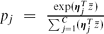 . The corresponding term in the posterior distribution is
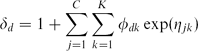
 . This term cannot be solved even after introducing the variational distribution q. Consequently, another variational distribution parameter δ is introduced for further approximation. We give the final inference form as follows. The details are given in Appendix B.

The optimization of Lagrangian over q(η) is obtained by setting  . Next, the optimization problem (7) can be converted into its dual by plugging the resultant q(η) into . For the standard normal prior for p 0(η) = N(0,I), the dual problem will be quadratic and standard QP solvers can be used to solve it. However, according to the principle of conjugate prior, q(η) is a normal distribution with a shifted mean as q(η) = N(λ,I), where
 . This can be taken into consideration to reformat the primal form of dual and it is solved by using existing multi-class SVM methods to get Lagrange multiplier μd and its duals (Zhu et al. Reference Zhu, Ahmed and Xing2009).
2.4 Relation detection
With the generative process, inference, and parameter estimation in place, ERD-MedLDA is ready to perform relation detection. The first step is to perform variational inference given the testing instances.
In classification, we estimate the probability of the relation type given topics and the response parameters, i.e., p(yd|z d1:dN, η). Using variational approximation described in the previous section, we can derive the prediction rule as F(y,z,η)=ηT f(y,z) where f(y,z) is a feature vector. Now, SVM can be used to derive the prediction rule (Zhu et al. Reference Zhu, Ahmed and Xing2009).

Recall that we make use of softmax regression in sampling relation types; consequently, the derivation rules are given as:

The term  , like in model learning, is intractable. Therefore, similar variational distributions are introduced. Namely, we use
 to approximate .
3 Data
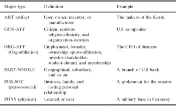
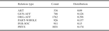
We use the ACE corpus (Phase 2, 2005) for training and evaluation. The ACE corpus has annotations for both entities and relations. The corpus has seven entity types, six major relations types, and twenty-three relation subtypes . In this work, we focus only on the six high-level relation types listed in Table 1. In addition to the six major types, we have an additional category – no relation (NO-REL) that exists between entities that are not related.
Relation types for ACE 05 corpus

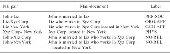
NEs within a sentence are paired, and all text in between and including the NEs is considered as a mini-document. The gold standard annotation of their ACE relation type, or NO-REL if no relation exists, forms the mini-document's label. For instance, consider the following sentence (all NEs are shown in italics):
John is married to Liz who works in Xyz Corp located in New York.
All NE pairs, the corresponding mini-documents, and their labels, constructed from this sentence, are listed in Table 2.
NE pairs, mini-documents, and labels for the sentence ‘John is married to Liz who works in Xyz Corp located in New York’

All relations in the ACE corpus are intra-sentential and hence we do not create NE pairs that cross sentence boundaries. Also, almost all positive instances are within two mentions of each other. Hence, we create NE pairs for only those NEs that have at most two intervening NEs in between. This gives us a total of 38,342 relation instances of which 32,640 are negative instances and 5912 are positive relation instances belonging to one of the six categories. The distribution of the six ACE categories is given in Table 3.
Distribution of relation types in the ACE corpus

4 Features
We explore the effectiveness of incorporating features into our system as well as the baselines. For this, we construct feature sets similar to Jiang and Zhai (Reference Jiang and Zhai2007) and Zhou et al. (Reference Zhou, Jian, Jie and Min2005). Three sets of features are employed: Bag of Words (BOW), Syntactic (SYN), and Composite (COMP).
4.1 Bag of words features (BOW)
The BOW feature captures all the words in our mini-document. Consider, for example, the following text snippet that reveals an affiliation relation (ORG-AFF) between X and the United States.
(1) X, the president of the United States [ACE relation type: ORG-AFF]
Notice that words such as ‘of’ can be indicative of the ORG-AFF relation. BOW features capture this lexical information. However, compared to traditional classification settings, there is a difference in how ERD-MedLDA employs these features. BOW features are trained as topics and then the discovered topics will be employed as features. Thus, words such as ‘of’ may fall into topic(s) %(that might also contain words like “founder”) that, in turn, would eventually contribute to the recognition of ORG-AFF class.
4.1 Syntactic features (SYN)
The SYN features are constructed to capture syntactic, semantic, and structural information of the mini-document. Let us consider the following text snippet where there is no relation between X and the United States:
(2) X, the president, visited the United States [ACE relation type: no relation]
Notice that even though examples 1 and 2 exhibit different relation types, they share a large number of words. Now, observe that the words that indeed differ between the two text snippets, ‘of’ and ‘visited,’ also differ in their part of speech: one is a preposition (IN), while the other is a verb (VBD). Thus, we include part of speech (POS) information of the words between two NEs to additionally clue the system to the type of relation that might exist between them.
We observed that the syntactic roles are also indicative of relationships between entities. For instance, in Example 1, X, the president, is the subject of the United States. We encode syntactic features to capture this information. These include:
• HM1: The head word of the first mention
• HM2: The head word of the second mention
• ET1: Entity type of the first entity
• ET2: Entity type of the second entity %SW:: ADDRESSED REV2.8 HERE
• M1: Mention type of the first entity
• M2: Mention type of the second entity
• #MB: Number of other mentions in between the two mentions under consideration
• #WB: Number of words in between the two mentions
4.3 Composite features (COMP)
The composite features (COMP) are similar to SYN, but they additionally capture order and dependencies between the features mentioned above. In particular, they capture structural information. Ordering of words are not captured by BOW or SYN. This feature exchangeability works for models based on random or seeded sampling (e.g., LDA) – as long as words sampled are associated with a topic, the hidden topics of the documents can be discovered. In the case of ERD, this assumption might work with symmetric relations. However, when the relations are asymmetric, ordering information is important. Besides exchangeability, LDA-based models also assume that words are conditionally independent. Consequently, the system cannot capture the knowledge that some mentions may be included in other mentions.
We overcome these limitations by explicitly encoding these information as COMP features. Composite features comprise of feature pairs indicating which of the two occurs first. These include:
• HM1HM2: Head word of mention 1 and head word of mention 2. This encodes what mention head word occurs first.
• ET12 : Ordered pair of mention entity type.
• ML12: Combination of mention levels.
• M1InM2: Flag indicating whether M1 is included in M2. This feature captures mention dependencies.
• M2InM1: Flag indicating whether M2 is included in M1.
5 Experiments
ERD-MedLDA is a LDA-based framework that uses maximum-margin learning. Thus, we need to verify if our MedLDA formulation does better than topic modeling alone and maximum-margin methods alone. For this, we compare ERD-MedLDA to both LDA and SVM. Comparison with SVM is straightforward as it is a supervised framework. However, as the basic LDA is unsupervised, the discovered topics are not tied to any particular class. Thus, for a fair comparison, we use a labeled variant of LDA, the LLDA (Ramage et al. Reference Ramage, Hall, Nallapati and Manning2009), as the baseline topic model system.
We use 80% of the instances for training and 20% for testing. The topic numbers and the penalty parameter of the cost function C are first determined for each of the models (wherever applicable) using the training data (the training data is split into training and validation sets). Best parameters are determined for the three conditions: (1) BOW features alone BOW, (2) BOW plus SYN features (PlusSYN), and (3) BOW plus SYN and COMP features (PlusCOMP). All systems achieved their overall best performance with PlusCOMP features (see Section 6.1 for a detailed analysis).
5.1 ERD-MedLDA setup
The number of topics for the LDA-based models are determined using the equation 2K 0 + K 1 following Zhu et al. (Reference Zhu, Ahmed and Xing2009) and K 1 = 2K 0. K 0 is the number of topics per class and K 1 is the number of topics shared by all relation types. The choice of topics is based on the intuition that the shared component K 1 should use all class labels to model common latent structure while non-overlapping components should model specific data characteristics from each class. The ratio of topics is based on the understanding that shared topics may be more than topics of each class. The specific numbers do not produce much variation in the final results. We experimented with the following number of topics: 20, 40, 70, 80, 90, 100, and 110. BOW, PlusSYN, and PlusCOMP configurations obtain the best performance for ninety, eighty, and seventy topics respectively.
Since SVMs are employed in the ERD-MedLDA implementation, we need to determine the penalty parameter of the cost function, C. We used five-fold cross-validation to locate the parameter C. The best values for C are 25, 28, and 30, respectively, for BOW, PlusSYN, and PlusCOMP configurations. We used a linear kernel as it is the most commonly used kernel for text classification tasks. Since ERD-MedLDA is run by sampling, the result may be different each time. We ran it five times for each setting and took the average as the final results.
5.2 Baselines
We employ the same features and the same settings for ERD-MedLDA, LLDA, and SVM wherever possible.
5.2.1 LLDA
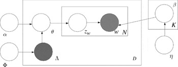
LLDA (Ramage et al. Reference Ramage, Hall, Nallapati and Manning2009) is a variation of sLDA. While the original LLDA model was designed for recognizing credit attribution, it can be easily used for relation detection. We recreate the plate diagram from the original paper in Figure 3 and briefly explain the LLDA model for relation detection as follows.
Graphical model of LLDA.

The relation types (Λ) generate the topic distribution parameter θ with α. Each document d is represented by a tuple consisting of a list of word indices wd = (w 1, . . ., wNd) and a list of binary relation type presence/absence indicators Λ(d) = (l 1, . . ., lK), where each wi ∈ {1, . . ., V} and each lk ∈ {0,1}. Nd is the document length, V is the vocabulary size, and K the total number of unique topic labels in the corpus.
Drawing the multinomial topic distributions over vocabulary βk for each topic k, from a Dirichlet prior η, is the same as that for traditional LDA. However, LLDA restricts θd to be defined only over the topics that correspond to its labels Λ(d). Since the word-topic assignments zi are drawn from this distribution, this restriction ensures that all the topic assignments are limited to the document's label. We refer the reader to the original paper for further details.
The setting of topics for LLDA is similar to ERD-MedLDA. As LLDA is also run by sampling, we ran it five times for each setting and took the average as the final results.
5.2.2 SVM
The SVM (Cortes and Vapnik Reference Cortes and Vapnik1995) baseline is a straightforward supervised system. We use the SVMlight implementation from (Joachims Reference Joachims1999). For for our task, labels are relation types and the training vector comprises of the features discussed in Section 4. Binary (presence/absence) features are used to overcome sparsity problems. In SVMlight, a grid search tool is provided to locate the best value for parameter C. The best C value for all three feature conditions, BOW, PlusSYN, and PlusCOMP, was found to be 1. All other settings are similar to those of ERD-MedLDA, including the linear kernel.
5.3 Results
We present the results of the three systems built using PlusCOMP, as all systems achieved their best overall performance using these features. Table 4 reports the precision, recall, and F-measure of the three systems averaged across all seven categories (the best numbers for each metric are highlighted in bold). Among the baselines, SVM has better precision, while LLDA has better overall recall. Here, we see that ERD-MedLDA outperforms LLDA and SVM across all metrics. Specifically, there is a four percentage point improvement in precision, two percentage point improvement in recall, and fifteen percentage point improvement in F-measure over the best performing baseline. This result indicates that our approach of combining topic models and maximum-margin learning is effective for relation detection.
Overall performance of the three systems

We performed t-tests to verify the significance of the improvements obtained by our system. The improvements obtained by ERD-MedLDA over SVM for recall and F-measure are highly significant (p < 0.001), while the improvement for precision is significant at p < 0.05. Comparing with LLDA, ERD-MedLDA's improvement for recall is significant at p < 0.1 while its improvements in precision and F-measure are significant at p < 0.001.
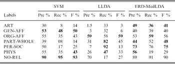
Now, looking at the results for each individual relationship category (see Table 5; the best numbers for each category and metric are highlighted in bold) we see that the F-measure for ERD-MedLDA is better than that for SVM for four out of the six ACE relation types; and better than the F-measure obtained by LLDA for all relation types except ORG-AFF. Specifically, comparing with the best performing baseline, ERD-MedLDA produces a F-measure improvement of twenty-seven percentage points for ART, three percentage points for PART-WHOLE, and fifty percentage points for PER-SOC. Also, for four of the six ACE relation types, ERD-MedLDA achieves the best precision. Even in the cases where ERD-MedLDA is not the best performer for a relation category, its performance is not very poor (unlike, for example, SVM for PART-WHOLE and LLDA for ART respectively).
Multi-class classification results with PlusCOMP for SVM, LLDA, and ERD-MedLDA for the six ACE 05 categories and NO-REL

Notice that LLDA has more difficulty with marginal classes such as ART and GEN-AFF. Interestingly, the NO-REL category reveals a sharp contrast in the performance of SVM and LLDA. NO-REL is a difficult, catch-all category that is a mixture of data with diverse distributions. This is a category where maximum-margin learning is more effective than MLE. Notice that ERD-MedLDA achieves performance close to SVM for this category. This is because, even though both LLDA and ERD-MedLDA model hidden topics and then employ the discovered hidden topics to predict relation types, ERD-MedLDA does joint inference of MLE and MME. This joint inference helps to improve the detection of NO-REL.
Finally, we also compare our system's results (using PlusCOMP features) with results of previous research. Much of the previous mainstream research has been carried out on previous versions of the ACE corpus (e.g., Bunescu and Mooney Reference Bunescu and Mooney2005; Jiang and Zhai Reference Jiang and Zhai2007; Qian et al. Reference Qian, Zhou, Kong, Zhu and Qian2008; Nguyen, Moschitti and Riccardi Reference Nguyen, Moschitti and Riccardi2009; Chan and Roth Reference Chan and Roth2011). Due to the difference in corpora, our results are not directly comparable to theirs. Relation extraction work by Khayyamian, Mirroshandel and Abolhassani (Reference Khayyamian, Mirroshandel and Abolhassani2009) on the ACE 2005 corpus is closest to our work. They use similar experimental settings: every pair of entities within a sentence is regarded to involve a negative relation instance unless it is annotated as positive in the corpus. A similar filter (they use a distance filter) is used to sift out unrelated negative instances. Their train/test ratio of data split is also the same as ours.
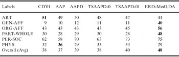
Khayyamian et al. (Reference Khayyamian, Mirroshandel and Abolhassani2009) employ classical kernel methods developed by Collins and Duffy (Reference Collins and Duffy2002) and only report F-measures over the six ACE relation types. For clarity, we reproduce their results in Table 6 and repeat ERD-MedLDA F-measures from Table 5 in the last column. The last row (Overall) reports the macro-averages computed over all relation types for each system. Here, we see that overall ERD-MedLDA outperforms all kernels. ERD-MedLDA also performs better than the best kernel for four of the six relation types.
F-measures for every kernel in Khayyamian, Mirroshandel and Abolhassani (Reference Khayyamian, Mirroshandel and Abolhassani2009) and ERD-MedLDA

6 Analysis
We incorporated an exponential family distribution into ERD-MedLDA model in order to make use of rich features. In this section, we analyze if indeed ERD-MedLDA effectively utilizes the variety of features listed in Section 4 in comparison with baseline methods. Additionally, as supervised topic models are designed to infer topic distributions indicative of the class, we inspect the topics learned by ERD-MedLDA to see if the inclusion of supervision has created topics biased towards relation types.
6.1 Feature incorporation
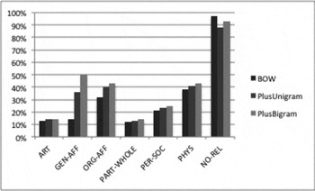
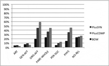
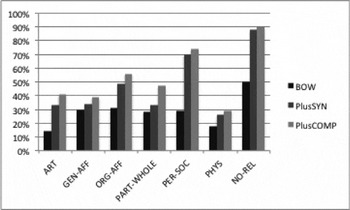
As mentioned previously, all three systems achieved their overall best performance with PlusCOMP features. Here, we analyze if informative features are consistently useful and if the systems can harness informative features consistently across all relation types. Figures 4–6 illustrate the F-measures for SVM, LLDA, and ERD-MedLDA respectively for the three conditions: BOW, PlusSYN, and PlusCOMP.
SVM F-meausres for three feature conditions.

LLDA F-meausres for three feature conditions.

MedLDA F-meausres for three feature conditions.

Let us first look at the best systems (based on F-measure) for each of the six ACE relation types in Table 5, and look at what feature set produces the best result for that system and relation. ERD-MedLDA is the best performer for ART, PART-WHOLE, and PER-SOC in Table 5. Figure 6 reveals that ERD-MedLDA's best performance for these relation types are obtained using PlusCOMP features. Similarly, SVM obtains the best F-measure for GEN-AFF and PHYS relations and Figure 4 shows that SVM achieves its best performance for these categories using PlusCOMP. We also see a similar trend with LLDA and the ORG-AFF relation type. These results corroborate intuition from previous research that informative features are important for relation type recognition. The only exception to this is the performance of SVM for NO-REL. This is not surprising, as the features we use are focused on determining true relation types and NO-REL is a mixture of all cases (and features) where relations do not exist.
Further analysis of the figures reveal that even though there is a general trend towards better performance with addition of more informative features, not all systems show consistent improvements across all relation types with the addition of composite features. That is, some systems get degraded performance due to feature addition. For example, in Figure 4, we see that the SVM with PlusCOMP features is outperformed by SVM with PlusSYN for ART and SVM with BOW for NO-REL. The gains from features are also inconsistent in the case of LLDA (Figure 5). While the LLDA system with PlusSYN features always improves over the one using BOW, the performance drops considerably when using PlusCOMP features for ART and GEN-AFF. On the other hand, ERD-MedLDA (see Figure 6) shows more consistent improvement for all relation types with the addition of more complex features. Also, the gains are more substantial. This is encouraging and opens up avenues for further exploration of richer features for ERD-MedLDA.
6.2 Topic discovery
Our goal in employing a supervised framework was to guide the topic discovery to topics useful for relation detection. In this section, we examine the topics discovered for each relation type and discuss the effects of varying the number of topics in our model.
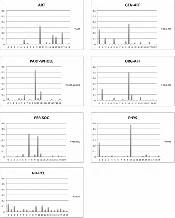
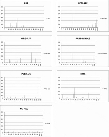
Figure 7 illustrates the topic distribution in ERD-MedLDA for the different relation types when twenty topics are used. The distributions are computed by averaging the expected latent representation of documents in each class. For all six ACE relation categories, we observe a sharp, sparse, and fast-decaying distribution over topics, indicating an affinity of the relation types for certain indicative topics. The NO-REL class, on the other hand, does not show this characteristic. Here, we see an almost uniform distribution over (almost) all topics. This is not surprising, as the NO-REL is a catch-all category comprising of various topics that do not correspond to the ACE relation types.
Topic distribution for all relation types and NO-REL with twenty topics.

Notice that Topics 0 and 10 are prominent across some relation types. Specifically, Topic 10 is prominent for all six ACE relation categories, and Topic 0 is prominent for GEN-AFF and PHYS categories. When we inspected the top features belonging to Topic 10, we discovered that it covered person-related and pronominal features such as I – I, I – you or I – my, he, he – he, they – he, them – I, and that. Intuitively, these features could indicate any one of the relation types. Topic 10 is in fact an indicator of a presence of an ACE relation – which also explains why Topic 10 is not seen in the NO-REL category.
Most relation types have distributions over additional topics that help in distinguishing them. For example, in addition to Topic 10, ART has a substantial percentage of distribution over Topics 14, 15, and 17. Similarly, ORG-AFF has noticeable distributions over Topics 1 and 11. The only exception is the PHYS category. PHYS has prominent distributions only over Topics 0 and 10, both of which are not unique to it alone. Not surprisingly, this affects the recognition of this category, as evidenced by the relatively low F-measures in Table 5. On the other hand, PER-SOC has a strong component of Topic 7, which is not seen in any other category. Consequently, it is recognized well by our system.
We observed that increasing the number of topics helps the system to obtain more distinct distributions for the relation types. Figure 8 illustrates the topic distribution when 110 topics are used. Notice that the topic distributions are more distinct for the ACE relation categories. However, we observed that if the number of topics is made too large, it can lead to overlapping topic distributions again. Finally, notice that NO-REL for 110 topics shows similar trend as that for twenty topics: it shows an almost uniform distribution over all topics.
Topic distribution for all relation types and NO-REL with 110 topics.

We also inspected the topics discovered by LLDA and basic LDA. LLDA assumes that the topic discovered is the relation type. Here too, supervision helped with tying the topics to the relation types. For example, family and wife were among the top features for PER-SOC, and weapons was a top feature for ART. However, we observed that the topics discovered in LLDA are relatively more general, and show more overlap between ACE relation categories. Additionally, it shows an even more broad topic distribution for NO-REL. In contrast, in ERD-MedLDA, though NO-REL has a broad topic distribution, not many topics overlap between NO-REL and the true relation types. Intuitively, this results in better NO-REL recognition in ERD-MedLDA as compared to LLDA.
Finally, topics discovered (and consequently, the features for those topics) by the basic LDA model were not clearly interpretable as indicative of the relation types. This is not surprising, as basic LDA does not incorporate supervision.
7 Related work
There has been significant research in relation detection and topic modeling. Our work straddles the two areas; we perform ERD within a topic modeling framework and our topic model is adapted to fit the requirements of the ERD task. The following sections discuss literature related to our work.
7.1 Relation detection
One of the popular approaches for ERD is kernel methods. The main advantage of kernel methods is the ability of exploiting large feature sets without an explicit feature representation. Some examples are dependency tree kernels (Culotta and Sorensen Reference Culotta and Sorensen2004) and shortest dependency path kernels (Bunescu and Mooney Reference Bunescu and Mooney2005). Other research in kernel methods include work form Zelenko, Aone and Richardella (Reference Zelenko, Aone and Richardella2003) that has exploited similarity measures over diverse features, convolution tree kernels (Zhao and Grishman Reference Zhao and Grishman2005; Zhang et al. Reference Zhang, Zhang, Su and Zhou2006), context-sensitive convolution tree kernels (Zhou et al. Reference Zhou, Zhang, Ji and Zhu2007), and dynamic syntax tree kernels (Qian et al. Reference Qian, Zhou, Kong, Zhu and Qian2008). Besides independent kernel functions, combinations of different kernel functions have also been explored. Nguyen et al. (Reference Nguyen, Moschitti and Riccardi2009) combine constituent and dependency trees and sequential structures with kernel methods. To fully exploit the potential of dependency tree, they also applied the partial tree kernel proposed by (Moschitti Reference Moschitti2006), and investigated the incorporation of dependency structure into rich sequence kernels.
Our method focuses on addressing the underlying semantics more directly than typical kernel-based methods. We try to capture structural information captured by kernel methods via explicit encoding of features. Further, the combination of MLE-based sLDA and MME-based SVM makes it possible for our model to directly employ rich kernel functions. The use of kernel functions in ERD-MedLDA is one of the directions for future work.
Chan and Roth (Reference Chan and Roth2011) employ constraints for relation detection using an integer linear programming (ILP) framework. Using this, they apply rich linguistic and knowledge-based constraints based on coreference annotations, a hierarchy of relations, syntacto-semantic structure, and knowledge from Wikipedia. In our work, we focus on capturing the latent semantics of the text between the NEs.
A variety of features have been explored for ERD in previous research (Miller et al. Reference Miller, Fox, Ramshaw and Weischedel2000; Kambhatla Reference Kambhatla2004; Zhou et al. Reference Zhou, Jian, Jie and Min2005; Jiang and Zhai Reference Jiang and Zhai2007; Zhou et al. Reference Zhou, Zhang, Ji and Zhu2008). Syntactic features such as POS tags and dependency path between entities; semantic features such as Word-Net relations, semantic parse trees, and types of NEs; and structural features such as which entity came first in the sentence have been found useful for ERD. For instance, Roth and Yih (Reference Roth and Yih2002) have applied a probabilistic approach to solve the problems of NE and relation extraction with the incorporation of all these features. Kambhatla (Reference Kambhatla2004) has employed maximum entropy models with diverse features including words, entity, and mention types and the number of words (if any) separating the two entities.
We too observe the utility of informative features for this task. However, exploration of the feature space is not the main focus of this work. Rather, our focus is on whether the models are capable of incorporating rich features. A fuller exploration of rich heterogeneous features is a topic for future work.
A closely related task is that of relation mining and discovery, where unsupervised and semi-supervised approaches have been effectively employed (Hasegawa et al. Reference Hasegawa, Sekine and Grishman2004; Jiang Reference Jiang2009; Mintz et al. Reference Mintz, Bills, Snow and Jurafsky2009). For example, Hasegawa et al. Hasegawa et al. (Reference Hasegawa, Sekine and Grishman2004) use clustering and entity type information, while Mintz et al. (Reference Mintz, Bills, Snow and Jurafsky2009) employ distant supervision. Our ERD task is different from these as we focus on classifying the relation types into predefined relation types in the ACE-05 corpus.
7.2 Topic models
Many researchers have explored extensions to the original LDA from Blei, Ng and Jordan Blei, Ng and Jordan (Reference Blei, Ng and Jordan2003), such as correlated topic models (Blei and Jordan Reference Blei and Jordan2006), LLDA (Ramage et al. Reference Ramage, Hall, Nallapati and Manning2009), sLDA (Blei and McAuliffe Reference Blei and McAuliffe2008), and discLDA (Lacoste-Julien, Sha and Jordan Reference Lacoste-Julien, Sha and Jordan2008). LDA-based models have been adapted and employed for a wide variety of tasks such as genomic profiling (Flaherty et al. Reference Flaherty, Giaever, Kumm, Jordan and Arkin2005) and image annotation (Wang, Blei and Li Reference Wang, Blei and Li2009). In NLP, they have been employed for review mining (Titov and McDonald Reference Titov and McDonald2008; Zhao et al. Reference Zhao, Jiang, Yan and Li2010), perspective analysis (Lin, Xing and Hauptmann Reference Lin, Xing, Hauptmann, Daelemans, Goethals and Morik2008), and key phrase extraction (Zhao et al. Reference Zhao, Jiang, He, Song, Achananuparp, LIM and Li2011). In this work, we adapt the MedLDA topic model from (Zhu and Xing Reference Zhu and Xing2010) and (Shan et al. Reference Shan, Banerjee and Oza2009) to incorporate rich features for the task of relation extraction.
The work on relation discovery from Hachey (Reference Hachey2006) is close to our work. However, Hachey uses LDA as a module in his system to reduce feature dimensions only, while our approach employs the LDA-based framework for full relation detection.
8 Conclusion and future work
In this work we presented ERD-MedLDA, a system for detecting entity relations based on topic models. Our approach was motivated by the idea that latent semantics of text, as discovered by LDA-based models, are useful for relation detection. For this, we reformulated ERD as a topic modeling task. To the best of our knowledge, this is the first work to make full use of topic models for relation detection.
Starting with MedLDA and mixed-membership models, we adapted them to the relation detection task. Specifically, we modified the optimization problem and incorporated an exponential family distribution for each feature. The resulting ERD-MedLDA model has the advantages of both maximum-margin and maximum likelihood methods and is also able to benefit from rich features.
Our experiments show that ERD-MedLDA achieves better overall performance than SVM-based and LLDA-based approaches across all metrics. Comparing with previous work from (Khayyamian et al. Reference Khayyamian, Mirroshandel and Abolhassani2009), which have employed diverse kernels, we showed that ERD-MedLDA has better overall performance.
We also experimented with different features and investigated the effectiveness of ERD-MedLDA in harnessing these features as compared to baseline methods. Our analysis showed that ERD-MedLDA is able to effectively and consistently incorporate informative features. Examination of the topic distribution obtained by our system shows that supervision indeed helps the model to learn topics biased towards relation types.
As a model that incorporates maximum-likelihood, maximum-margin, and mixed-membership learning, ERD-MedLDA has the potential of incorporating rich kernel functions or conditional topic random fields (Zhu and Xing Reference Zhu and Xing2010). These are some of the promising directions for our future exploration.
Appendix A: Variational inferences
We can derive the variational inferences for (4) as follows. Based on Figure 2, for each data point wd, yd, the expected value of joint probability of Ls can be factored as:

The second term of (5),  is the variational form of the original log-likelihood form. The expanded form of that term is:

where γd is a K-dimensional vector of Dirichlet parameters, and each φdn is a categorical distribution over K topics. Namely, γd is the approximation of θ, and φdn is the approximation of zdn. Denoting the lower bound for each data point (wd, yd) with L(γd, φd; α, β, q(η)), (5) can be expanded as:

Appendix B: Parameter estimation
Without loss of generality, the following equations are for softmax distribution. The results remain similar for multi-class logistic regression after taking into account the number of elements in series summations. Hence, the probability mass of relation type yd given zd and η is:

Accordingly, the last term in (A3) is:

Even after introducing the variational distribution q, the above equation cannot be efficiently computed. Consequently, further approximation must be done. Thus, a new variational parameter δ is introduced to obtain a further lower bound for it. Specifically, besides Jensen inequality, another inequality, namely,  (Minka Reference Minka2003; Shan et al. Reference Shan, Banerjee and Oza2009), is used here to lower bound the term as:

Thus, with the addition of another variational parameter, δ, maximizing the lower-bound Lagrange function (8) with respect to the variational parameters will now give the update equation of γd, φd, η, and δd. The update rule of δd is similar to γd and φd. A simple partial derivation of (8) over δ will give its update equation as:
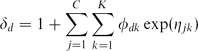
As we see from (B3), δ and φ are coupled together now. Hence, in the update rule of δ, φ is part of it. Consequently, the update rule of φ is not separate from δ.