2.a. Regional tectonics

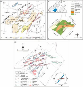
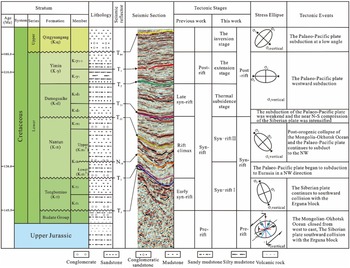
The Hailar Basin is located in the Erguna block between the Tahe–Xiguitu suture zone and the Derbugan Fault (Fig. 1a). According to the deformational characteristics and the rate of rifting, the basin is the result of three stages, including pre-rift (before K₁t sedimentation), syn-rift (K₁t–K₁d sedimentation) and post-rift phases (K₁y sedimentation) (Fig. 2; Zhou et al. Reference Zhou, Ji, Pigott, Meng and Wan2014). Nevertheless, the division of the structural evolution stages in the Hailar Basin has always been controversial because the multiphase stress field has played an important role in the basin’s evolution (Song et al. Reference Song, Liu, Wang, Gao and Liu2019).

Fig. 1.

(a) Regional structure background map after Meng et al. (Reference Meng, Wan and Zhu2013). (b) Structural location of the study area (B: basin; JD: Zhalainor Depression; CU: Cuogang Uplift; BD: Bell Lake Depression; BU: Bayan Mountain Uplift; HD: Huhe Lake Depression). (c) General structural units in the Beier Depression. (d) Structural map of the Beier Depression showing the major faults, well locations and oil accumulations. Rose diagram of the major faults.

Fig. 2.

Stratigraphy of the Beier Depression in the Hailar Basin. Stratigraphic classification modified after Jia et al. (Reference Jia, Liu, Miao, Fang, Zhou, Meng, Chen, Yan and Yang2014) and Ji et al. (Reference Ji, Ge, Wang, Yang, Zhao, Bi and Dong2016). The lithology of stratigraphic units is from Meng et al. (Reference Meng, Wan and Zhu2013). The stress ellipse evolution data are derived from Liu et al.(Reference Liu, Zhou, Tang, Wu, Li, Zhu, Jiang and Liu2017) and Song et al. (Reference Song, Liu, Wang, Gao and Liu2019). To illustrate the structural evolution clearly, N₁₄ is defined in this paper.

Previous works have put forward evidence to develop the geodynamic model of the study area during the Late Jurassic to Early Cretaceous: The superposition of post-orogenic lithospheric extension caused by the effect of Mongolia–Okhotsk Ocean closure and back-arc extension related to the Palaeo-Pacific plate westward subduction (Meng et al. Reference Meng, Xu, Yang, Qiu, Li and Zhu2011; T Wang et al. Reference Wang, Guo, Zhang, Yang, Zhang, Tong and Ke2015; Ji et al. Reference Ji, Ge, Wang, Yang, Zhao, Bi and Dong2016; Liu et al. Reference Liu, Zhou, Tang, Wu, Li, Zhu, Jiang and Liu2017; Song et al. Reference Song, Liu, Wang, Gao and Liu2019). In the Late Jurassic, the Mongolia–Okhotsk Ocean closed from west to east in a scissor-type pattern, forming a NE-trending suture zone (Meng et al. Reference Meng, Xu, Yang, Qiu, Li and Zhu2011; Xu et al. Reference Xu, Xu and Meng2011). Simultaneously, the Siberian plate collided southward with the Erguna block, resulting in sinistral transpression along the Mongolia–Okhotsk Ocean suture zone and forming NE-striking strike-slip faults (the Derbugan fault system) within the Erguna block (Zheng et al. Reference Zheng, Zhou and Jin2009; Meng et al. Reference Meng, Wan and Zhu2013). During the early Early Cretaceous (K₁t–K₁n sedimentation), the NNW–SSE- to NW–SE-trending extensional stress field developed in the Hailar Basin related to the post-orogenic collapse of the Mongolia–Okhotsk Ocean and the Palaeo-Pacific plate subducted to the NW (Parfenov et al. Reference Parfenov, Popeko and Tomurtogoo2001; Sorokin et al. Reference Sorokin, Kudryashov and Sorokin2002, Reference Sorokin, Kudryashov and Sorokin2003, Reference Sorokin, Kudryashov and Sorokin2005; W Wang et al. Reference Wang, Guo, Zhang, Yang, Zhang, Tong and Ke2015; Song et al. Reference Song, Liu, Wang, Gao and Liu2019). Subsequently, the subduction of the Pacific plate weakened, and the nearly N–S-trending compression of the Siberian plate continued to strengthen (Zhang et al. Reference Zhang, Ge and Wu2006; Xu et al. Reference Xu, Xu and Meng2011). During the late Early Cretaceous (K₁y sedimentation), the stress field of the Hailar Basin changed from NW–SE- to E–W-trending in conjunction with the westward subduction of the Palaeo-Pacific plate and the thermal subsidence after rifting (Tang et al. Reference Tang, Xu, Wang, Zhao and Li2015; Song et al. Reference Song, Liu, Wang, Gao and Liu2019). Finally, a compressive environment formed by the Palaeo-Pacific plate subducted to the NW at a low angle at the end of the late Early Cretaceous (Liu et al. Reference Liu, Wan, Ren, Li, Zhang and Liu2006; Song et al. Reference Song, Liu, Wang, Gao and Liu2019).

2.b. The Beier Ddepression

The Beier Depression is located in the southern part of the Bell Lake Depression in the Hailar Basin, next to the Wuerxun Depression in the northeast, and is more than 50 km long in the NE–SW direction (Fig. 1b). Since the late Mesozoic, the Beier Depression has experienced multiphase tectonic activities and comprises seven NE-trending structural units, namely, the Beixi monocline zone, Beixi sag, Holodomor fault nose zone, Beibei sag, Sudeerte fault tectonic belt, Beizhong sag and Beidong monoclinic zone (Fig. 1c). Tectonically, the Beier Depression is a half-graben under the control of ENE- and NE-trending major faults, characterized by faulting in the east and deposition in the west (Fig. 1d).

2.c. Stratigraphy

The structural layer of the Beier Depression can be divided into the basal structural layer, the rifting structural layer, the fault-depression transformation structural layer, and the depression structural layer (D Yu, unpub. MSc thesis, Northeast Petroleum Univ., Daqing, 2010) based on the relations involving the three seismic reflection unconformity surfaces T₅, T₂₂ and T₀₄. The basal structural layer refers to the Budate Group, which is dominated by low-grade metamorphic rocks overlain by interbedded volcanic and clastic rocks (Meng et al. Reference Meng, Wan and Zhu2013; Zheng et al. Reference Zheng, Mao, Chen and Zhu2021; Fig. 2). The rifting structural layer and the fault-depression transformation structural layer, which is the focus of this study, consist of the Tongbomiao Formation (K₁t), Nantun Formation (K₁n), Damoguaihe Formation (K₁d) and Yimin Formation (K₁y) from bottom to top.

The lithostratigraphy of the study area has been illustrated by many researchers (Meng et al. Reference Meng, Wan and Zhu2013; Zhou et al. Reference Zhou, Ji, Pigott, Meng and Wan2014; Chen et al. Reference Chen, Gao, Wu, Qu, Liu, Bai and Wang2016; Zheng et al. Reference Zheng, Mao, Chen and Zhu2021). The Tongbomiao Formation (250–700 m thick) is dominated by tuff sandstone and andesite in the lower part and mudrock inclusions to thick sandstone conglomerates in the upper part (Fig. 2). The Nantun Formation (200–700 m) is dominated by medium-grained sandstone interbedded with mudstone units (Fig. 2). The Damoguaihe Formation is relatively thick (450–1400 m) and characterized by sandy mudstone and mudstone units (Fig. 2). The Yimin Formation (200–1300 m) mainly consists of silty mudstone and sandy mudstone overlain by mudstone units (Fig. 2). The depression structural layer refers to the Late Cretaceous Qingyuangang Formation (100–300 m), which is dominated by conglomeratic sandstone and mudstone units. Characterizing the lithological variation in stratigraphy is of value for understanding the evolution of normal faults under a multiphase stress field (Jackson & Rotevatn, Reference Jackson and Rotevatn2013; Deng & McClay, Reference Deng and McClay2019).

3.a. Dataset

This study is based on a high-resolution, 3D seismic survey, which covers a total area of 2600 km² of the Beier Depression (Fig. 1c, d). The dominant frequency varies with depth and averages c. 50 Hz above the depth of the 1.5 s two-way travel time (TWT), yielding a vertical resolution of ∼10 m. The spatial resolution is approximately equivalent to the in-line and cross-line spacing of 25 m. The 3D seismic data were interpreted using Landmark software in conjunction with the relationship between the stratigraphic data from drill holes and the seismic reflection package contained in the synthetic seismic record. Ten major faults were interpreted in the study area. Eight key seismic horizons have been interpreted: T₀₄, T₁, T₂, T₂₁, T₂₂, N₁₄, T₃ and T₅ (Fig. 2). T₀₄, T₂₂ and T₅ are strong and continuous representatives of three unconformity surfaces in the study area. Other seismic horizons were mapped across the study area to constrain the throw distribution on the fault surfaces (Fig. 2). The faults were described in detail based on a comparison of the discontinuous characteristics of seismic reflection waves.

4.a. Fault geometric characteristics

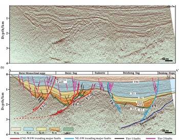
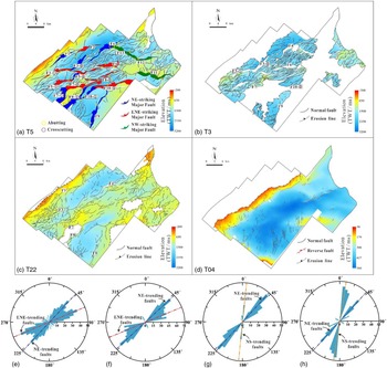
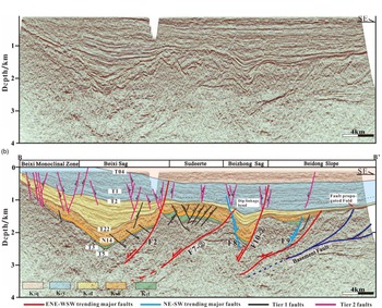
The 2D transect in Fig. 3 shows that major faults are mostly NW dipping in the Beier Depression, bounding the K₁d–K₁t growth packages (T₂–T₅ in Fig. 3). Additionally, some major faults significantly change directions along their lengths. Based on the seismic data, three extensional major fault populations can be distinguished on the base K₁t horizon map (T₅) (Fig. 4a): (i) NE–SW-trending fault array, (ii) ENE–WSW-trending fault array and (iii) NW–SE-trending fault array. The NE–SW-trending fault array is located at the edge of the study area and is labelled F1, F3-②, F4, F5-②, F7-①, F8-①, F9 and F10-①. The ENE–WSW-trending fault array is best developed in the centre of the study area and is labelled F2, F3-①, F5-①, F6, F7-②, F8-② and F10-②.There are only three NW–SE-trending faults located in the northeastern part of the study area, labelled F11, F12 and F13. Because it was subjected to intense erosion during the later period, the NW–SE-trending fault array was not used as the target of this study (Fig. 4). Nonetheless, minor faults can be characterized on the base K₁t, K₁n, K₁d and K₂q horizon maps (T₅, T₃, T₂₂ and T₀₄), which are predominantly NE–SW to ENE–WSW trending, with a few of them N–S trending (Fig. 4a–d).

Fig. 3.

(a) Uninterpreted and (b) interpreted inline 3D seismic sections in the south (see Fig. 1d for the locations of the sections).

Fig. 4.

TWT structure map and rose diagrams of four key horizons. T₅ time-horizon map (a, e), T₃ time horizon map (b, f), T₂₂ time-horizon map (c, g) and T₀₄ time horizon map (d, h), showing map view fault geometries and fault orientations. The NE–SW-trending faults strike 40–50°, and the ENE–WSW-trending faults strike 60–70°. The number of NE- and ENE-trending faults decreases upward.

4.a.1. NE–SW-trending fault array

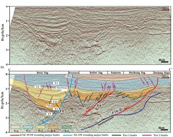
In map view, the NE–SW-trending faults are characterized by a broadly spaced curvilinear pattern and have strike lengths of 10–24 km (Fig. 4a). All of the NE–SW-trending faults can offset K₁t–K₁d and reach the T₂₂ interface (Fig. 4c). The fault surfaces in the profile are steep and straight, with dips to the NW and SE at angles of 70–85° (Figs 3, 5 and 6). Subtle wedge-shaped growth packages for the T₂–T₅ interval, especially the T₂–T₂₂ interval, can be observed in the hangingwall of the NE–SW-trending faults (Figs 3, 5 and 6), and the greatest increase in thickness for the T₂–T₂₂ interval is observed across fault F4 (Fig. 6).

Fig. 5.

(a) Uninterpreted and (b) interpreted inline 3D seismic sections in the middle (see Fig. 1d for the locations of the sections).

Fig. 6.

(a) Uninterpreted and (b) interpreted inline 3D seismic sections in the north (see Fig. 1d for the locations of the sections).

4.b. Fault displacement characteristics

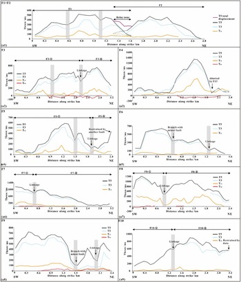
Figure 7a shows examples of fault displacement variations along fault strikes for ten major faults (F1–F10) in the study area. All of the major faults show maximum displacement at the base K₁t horizon along the entire length of the faults, suggesting that they may be syn-rift, pre-rift or ‘basement’-involved faults, whose displacement is greatest at the deepest horizons and decreases upward (Pongwapee et al. Reference Pongwapee, Morley and Wonin2019). In general, most major faults are fault segments of larger segmented fault arrays, and the continuity of the composite displacement profile of F1 and F2 shows that they interact with each other in relay zone. Notably, the displacement pattern of F2 shows approximately C-shaped profile, with the maximum displacement in the fault centre and the minimum displacement near the fault tips, indicating that F2 is an individual fault segment (Fig. a7). For the other faults, the T–x plots exhibit displacement maxima at the T₅ and T₃ interfaces, separated by a displacement minimum in between, indicating that the faults occurred as a result of the linkage of two or more fault segments (Fig. 7(a2), (a4), (a6), (a7), (a9)) or as branches of minor (Fig. 7(a5), (a8)) or major nearby faults (Fig. 7(a3)). The points of low displacement correspond to relay zones or branch points (Walsh et al. Reference Walsh, Bailey, Childs, Nicol and Bonson2003). Additionally, at the T₀₄ interface, the throws of F3, F4 and F8 show negative values (Fig. 7(a2), (a3), (a7)), indicating that the study area changed from an extension stress field to a compression stress field and that some major fault reactivation occurred during this period.

Fig. 7.

(a) T–x plots for major faults, showing fault segment displacements for the T₅, T₃, T₂₂ and T₀₄ interfaces (location is shown in Fig. 4a). Grey bars represent the segment positions.

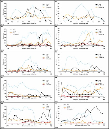
Figure 7b represents the interval displacement along major faults and uses the T–x plots to more clearly show how displacement evolves along the faults, and interval displacement is defined as the subtracting values of the shallower horizon from those of the deeper horizon (Morley et al. Reference Morley, Gabdi and Seusutthiya2007). Positive values imply typical growth fault characteristics and fault motion during the time of the interval. Any negative value is displayed as zero on the plots and suggests that particular area of the fault experienced displacement before or after deposition of the interval. These patterns suggest all of the major faults were active during deposition of the K₁t–K₁d Formations (Fig. 7b). The K₁n Formation shows greater displacement than the others. The interval displacement of some faults is equal or close to zero in the K₁d Formation, indicating that no growth occurred during that interval (Fig. 7b).

Fig. 7.

(b) Interval displacement plots for major faults; interval displacement is the product of subtracting values of the shallower horizon from the deeper horizon (Morley et al. Reference Morley, Gabdi and Seusutthiya2007).

4.c. Fault growth analysis

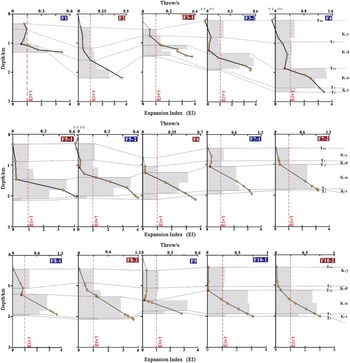
Determining when the major faults formed is essential to analysing the basin evolution process. T–z profiles not only define the fault activities during different periods but also provide information on the nucleation, propagation, segmentation and connection of a fault. Moreover, combined with changes in the expansion indices, this information can identify the periods of fault growth (Morley et al. Reference Morley, Gabdi and Seusutthiya2007; Baudon & Cartwright, Reference Baudon and Cartwright2008 a, b, c). Hence, T–z profiles and expansion indices (Fig. 8) were plotted to understand the timing of fault activities. The results show that the highest displacement of major fault segments F1–F10 occurs at the base K₁t horizon and decreases upward (Fig. 8), with expansion indices greater than 1.0 in K₁n and K₁t, coinciding with the K₁n and K₁t growth packages (T₂₂–T₃ and T₃–T₅ in Fig. 3). Notably, compared to K₁n, the growth packages are not obvious across the fault at K₁t, and it is likely that the high displacement is a sign of upward propagation of the basement faults developed in the Late Jurassic (Deng & McClay, Reference Deng and McClay2019).

Fig. 8.

Throw–depth (T–z) plots and expansion index for major faults (red labels represent the ENE–WSW-trending faults; blue labels represent the NE–SW-trending faults).

Major faults in the same strike show similar vertical displacement patterns. It is worth noting that the local throw minima of NE–SW-trending major faults (F1, F3-②, F4, F5-②, F7-①, F8-①, F9 and F10-①) are seen at the T₂₂ interface, in accord with EI values less than 1.0 in K₁d (Fig. 8), while the other major faults, oriented in an ENE–WSW direction (F2, F3-①, F5-①, F6, F7-②, F8-② and F10-②), are not. The local throw minima in the throw–depth (T–z) profiles correspond to incompetent mud-rich intervals, which are interpreted to be segmented zones controlled by dip linkage (Figs 5, 6), suggesting that the NE–SW-trending major faults were inactive during K₁d and reactivated or initiated later and propagated downward. Thus, there was a pronounced change in major fault activities between different orientations. As observed from the expansion indices, a third episode of fault growth can be seen in F3-②, F4, F5-②, F7-①, F8-① and F9 at the end of the K₁y sedimentary period (Fig. 8), which corresponds to the post-rifting inversion stage (Liu et al. Reference Liu, Wan, Ren, Li, Zhang and Liu2006; Song et al. Reference Song, Liu, Wang, Gao and Liu2019).

5.a. Phase 1: syn-rift I (T₅–N₁₄)

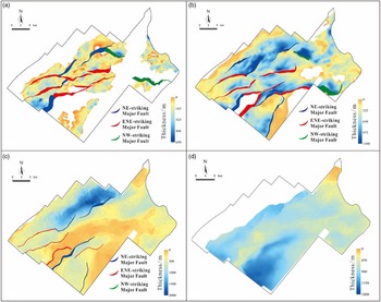
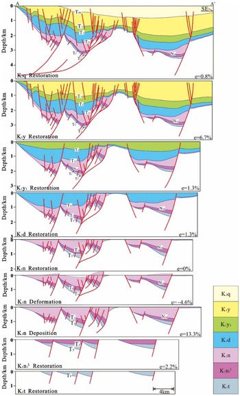
The Beier Depression initiated in the Early Cretaceous along NE–SW- to ENE–WSW-trending faults (Figs 3, 9), followed by a NNW–SSE-trending regional extension pattern during syn-rift I related to the post-orogenic collapse of the Mongolia–Okhotsk Ocean (Tang et al. Reference Tang, Xu, Wang, Zhao and Li2015; W Wang et al. Reference Wang, Guo, Zhang, Yang, Zhang, Tong and Ke2015). The deformation in the study area is mainly accommodated by a domino extensional structural style, and major faults were active during this stage based on their wedge-shaped hangingwall T₅–N₁₄ growth packages in the seismic section (Fig. 10). According to the major-fault expansion index values of slightly more than 1.0 (Fig. 8), K₁t was a period of weak extension, and major faults were active on a small scale. On the isochron map, there is only slight thickening near some ENE–WSW-trending faults (F2, F5, F6 and F7 in Fig. 9a). The explanation for this result is that the orthogonal extensional deformation of ENE–WSW-trending faults produced a greater amount of extension displacement than the oblique extensional deformation of the underlying NE–SW-trending faults.

Fig. 9.

Isochron map for (a) K₁t, (b) K₁n, (c) K₁d and (d) K₁y, with corresponding major fault maps of the base horizons.

Fig. 10.

A schematic model for the geological evolution of the study area in regional line A–A’ (the location of this line is shown in Fig. 1d).

Between phase 1 and phase 2, the lower part of the first member of K₁n, with uniform thickness covering the whole area, was deposited (orange colour fill in Figs 5, 6), and the top interface (N₁₄) is an unconformity (Meng et al. Reference Meng, Xu, Yang, Qiu, Li and Zhu2011). Generally, in the syn-rift stage, the strata are thickest close to the faults and gradually thin away from the faults, in other words, the sedimentation of the strata is obviously controlled by the faults (Song et al. Reference Song, Liu, Wang, Gao and Liu2019). However, the characteristics of the depression sedimentary sequence that appeared in the syn-rift stage indicate that tectonic movement quiesced during this period, matching the period during which the Pacific plate was subducted into the Eurasian plate and resulted in the transformation of the regional tectonic system from the Mongol–Okhotsk tectonic domain to the Pacific tectonic domain (Tang et al. Reference Tang, Xu, Wang, Zhao and Li2015; Ji et al. Reference Ji, Ge, Wang, Yang, Zhao, Bi and Dong2016). The combination of geological phenomena and tectonic setting shows that the sedimentary period of the lower part of the first member of the K₁n was a rifting transition stage.

5.b. Phase 2: syn-rift II (N₁₄–T₂₂)

After the rifting transition stage, the extension direction changed from NNW–SSE to NW–SE related to the subduction of the Palaeo-Pacific plate to the NW (Parfenov et al. Reference Parfenov, Popeko and Tomurtogoo2001; Sorokin et al. Reference Sorokin, Kudryashov and Sorokin2002). The comparison of isochron maps of the T₅–N₁₄ interval with the N₁₄–T₂₂ interval shows the very different deformation patterns exhibited by the depocentres (Fig. 9). The N₁₄–T₂₂ interval shows that the strata thickness increases significantly, with NE–SW- to ENE–WSW-trending depocentres near the major faults (Fig. 9b). These findings show that the thickness of strata close to the major faults is the largest in the profile, revealing that the development of strata is controlled by activity along the faults (Fig. 10). Additionally, the expansion indices of major faults increased significantly during the sedimentary period of K₁n (Fig. 8), coinciding with the isochron maps (Fig. 9b), indicating that the extension was intense. Furthermore, the major faults trending ENE–WSW were probably mildly active, as suggested by the thickness variations across the faults being less than that of the NE–SW-trending faults on the isochron maps (Fig. 9b).

At the end of phase 2, there is a high-angle truncation relationship between K₁d and K₁n (T₂₂ unconformity) (Figs 3, 5 and 6), which indicates that strong tectonic uplift, deformation and inversion-related erosion occurred in the depression in the late depositional stage of K₁n. Most of the faults terminated upward at the T₂₂ interface (Figs 3, 5 and 10) because the overlying K₁d strata have high mud contents and their displacements were absorbed by mud-bearing strata. The results of 2D basin structural reconstruction of K₁n₂ show that the study area experienced uplift and severe erosion (Fig. 10), confirming the above analysis. Similarly, previous works have shown that there was compression in this sedimentary period (Shen et al. Reference Shen, Li, Chen, Yin and Zhang2005; Sun et al. Reference Sun, Lu, Zhang, Du and Xu2011; Zhang et al. Reference Zhang, Meng and Qi2012; Gao et al. Reference Gao, Liu, Wu, Xu, Huang, Mei and Sun2014) owing to the weakening subduction of the Pacific Ocean and the strengthening of nearly N–S compression induced by the Siberian plate (Ji et al. Reference Ji, Ge, Wang, Yang, Zhao, Bi and Dong2016). This explanation matches the pattern that can be traced to adjacent depressions. For example, a large number of compressive structures can be found in the lower strata of K₁d in the Wuerxun Depression depending on the 3D seismic interpretation (Liu et al. Reference Liu, Liu, Wang, Wu, Zhu and Wan2009), which is next to the northeastern Beier Depression (Fig. 1b), and compressive structures were found on outcrops at the edge of the Hailar Basin during the field geological survey (Sun et al. Reference Sun, Lu, Zhang, Du and Xu2011).

5.c. Phase 3: post-rift (T₂₂–recent)

In K₁d and K₁y, the Beier Depression entered the post-rift stage. Fault control was weakened, and thermal subsidence began to enhance during this stage. Two depocentres were located in the northwest and southeast, whereas the strata between them were thin, corresponding to the location of the Sudeerte fault tectonic belt (Fig. 1b) for the T₂₂–T₀₄ interval (Fig. 9c). According to the characteristics of the basin, the post-rift stage can be further divided into three phases: (i) the thermal subsidence stage (T₂₂–T₁ interval), (ii) the extension stage (T₁–T₀₄ interval) and (iii) the inversion stage (T₀₄–recent)

During the T₂₂–T₁ interval, the activity of the major faults was mostly weak except for some individual faults. The central part of the Beier Depression is characterized by depression and flexural deformation (Fig. 10). Meanwhile, the deposition rate exceeded the subsidence rate during this period (Song et al. Reference Song, Liu, Wang, Gao and Liu2019), resulting in the spreading of the deposition distribution throughout the depression in the profile (Fig. 3). Thickness changes across faults may be due to differential thermal subsidence over the buried rift topography (Deng et al. Reference Deng, Fossen, Gawthorpe, Rotevatn, Jackson and Fazlikhani2017).

During the T₁–T₀₄ interval, the direction of the stress field changed from NW–SE to E–W (Tang et al. Reference Tang, Xu, Wang, Zhao and Li2015; Ge et al. Reference Ge, Zhu, Wang, Jones and Chen2018), and the major faults trending NE–SW were characterized by prevalent reactivation, as clearly shown by the T–z plots and the transverse cross-sections (F1, F3, F4, F8 and F9 in Figs 3, 5, 6 and 8). Notably, there is a fault-propagated fold around F10 oriented ENE–WSW in the seismic section (C–C’ profile in Fig. 6), probably due to the reactivation of the basement normal fault in essence. Simultaneously, in map view, a large number of NE–ENE-trending normal minor faults controlled by the pre-existing major faults were formed, and a series of N–S-trending newly formed minor faults can be observed in the southwestern part of the study area (Fig. 4c). Minor faults propagate downward and intersect the major faults in the combination of Y-shaped and V-shaped styles in the cross-sections (Figs 3 and 10). In detail, F3, F4 and F8 show stronger activity among these reactivated major faults based on their expansion index values greater than 1.0 (Fig. 8).

During the T₀₄–recent interval, the study area experienced a second-stage tectonic inversion due to the low-angle northwestern subduction of the Pacific plate (Tang et al. Reference Tang, Xu, Wang, Zhao and Li2015; Song et al. Reference Song, Liu, Wang, Gao and Liu2019). The T₀₄–recent interval is different from the underlying T₂₂–T₀₄ interval in two ways. First, the depocentre has been reorganized, and the T₂₂–T₀₄ interval shows a NE–SW-trending depocentre in the NW corner, while T₀₄–recent shows a depocentre in the SE corner. The northwestern depocentre is replaced by an absence of basin sediment (Fig. 9d). Second, there are some local reverse faults oriented NE (Fig. 4d).

6.a. Interpretation of the origin of major faults in the Beier Depression

There are three groups of major strike faults in the study area (Fig. 4a). Our observations suggest that they developed at the same time and that all of them have a high displacement but a low expansion index value at depth (Fig. 8). These findings indicate that the major faults present in the Beier Depression are unlikely to be the result of synsedimentary faults but tend to be strongly influenced by pre-existing fabrics. An example from the pre-rift structural layer of the basement fault is shown in Figuress 3 and 5. Hence, it is essential to consider how the pre-rift geology has influenced the structure of the Beier Depression.

Previous studies demonstrated that NE China or even greater NE Asia underwent a substantial intracontinental deformation process related to the evolution of the Mongol–Okhotsk tectonic regime and the Palaeo-Pacific tectonic regime in the late Mesozoic (Parfenov et al. Reference Parfenov, Popeko and Tomurtogoo2001; Sorokin et al. Reference Sorokin, Kudryashov and Sorokin2002, Reference Sorokin, Kudryashov and Sorokin2003, Reference Sorokin, Kudryashov and Sorokin2005; Zhu et al. Reference Zhu, Chen, Wu and Liu2011, Reference Zhu, Yang and Wu2012; W Wang et al. Reference Wang, Guo, Zhang, Yang, Zhang, Tong and Ke2015; Song et al. Reference Song, Liu, Wang, Gao and Liu2019). In recent years, an increasing number of systematic studies have shown that the closure of the Mongol–Okhotsk tectonic regime had a stronger influence than the Palaeo-Pacific tectonic regime during the Late Jurassic period (Dong et al. Reference Dong, Zhang, Long, Yang, Ji, Wang, Hu and Chen2007, Reference Dong, Ge, Yang, Xu, Zhang, Bi and Liu2016; Meng et al. Reference Meng, Liu, Cui, Gao, Liu and Tong2014; Shi et al. Reference Shi, Zheng, Yao, Li, Cui, Gao, Gao, Xu and Han2015; Tang et al. Reference Tang, Xu, Wang, Zhao and Li2015, Reference Tang, Xu, Wang and Ge2018). In the Late Jurassic, the Mongolia–Okhotsk Ocean closed from west to east, forming a NE-trending suture zone (Gou et al. Reference Gou, Sun, Zhao, Ren, Zhang, Fu, Wang and Wei2010; Meng et al. Reference Meng, Xu, Yang, Qiu, Li and Zhu2011; Xu et al. Reference Xu, Xu and Meng2011). Then the collision between the Siberian plate and the Erguna block resulted in sinistral transpression along the NE-trending suture zone and formed NE-trending strike-slip faults and strike-slip-associated structures (Fig. 2). These structures include (i) ENE–WSW- to E–W-trending compressional thrust structures, (ii) NE-trending R shear fractures, (iii) NW-trending R’ shear fractures and (iv) N–S-trending T extension fractures (Meng et al. Reference Meng, Wan and Zhu2013).

A number of studies have documented that the pre-existing fabric plays an important role in the formation and evolution of the fault system in rift basins (Smith & Mosley, Reference Smith and Mosley1993; McClay & White, Reference McClay and White1995; Morley, Reference Morley1999, Reference Morley2002, McClay et al. Reference McClay, Dooley, Whitehouse and Mills2002; Morley et al. Reference Morley, Haranya and Phoosongsee2004; Deng et al. Reference Deng, Fossen, Gawthorpe, Rotevatn, Jackson and Fazlikhani2017; Song et al. Reference Song, Liu, Wang, Gao and Liu2019). Fault systems tend to develop on weak pre-existing fabrics (Smith & Mosley, Reference Smith and Mosley1993, Tong et al. Reference Tong, Nie, Meng, Zhang and Li2009). The Hailar Basin lies adjacent to the southern edge of the Mongol–Okhotsk suture zone (Fig. 1). Internal to the basin, ENE–WSW-, NE–SW- and NW–SE-trending faults are present in the Beier Depression, and in addition to the above orientations, N–S-trending major faults exist on the western margin of the Wuerxun Depression (Meng et al. Reference Meng, Wan and Zhu2013). Moreover, ENE–WSW-trending major faults have smaller dip angles (lower than 30°) than the other trend faults in the profile (Fig. 6), similar to the characteristics of thrust faults at depth. Temporally, the deformation time of the major faults coincides with the closure of the Mongolia–Okhotsk Ocean (Song et al. Reference Song, Liu, Wang, Gao and Liu2019). On this basis, we consider that the major faults may have originated from strike-slip-associated structures, which were pre-existing fabrics, and then reactivated, propagating upward under NNW–SSE- to NW–SE-trending extensional regimes in the Late Jurassic.

6.b. Growth history of non-collinear major faults

6.b.1. Classification of faults growth

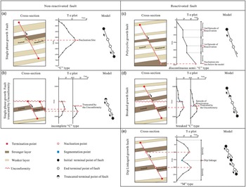
Normal faults can be defined as non-reactivated faults or reactivated faults depending on their growth mechanisms (Osagiede et al. Reference Osagiede, Duffy, Jackson and Wrona2014) and throw distribution pattern (Walsh et al. Reference Walsh, Nicol and Childs2002, Reference Walsh, Bailey, Childs, Nicol and Bonson2003; Giba et al. Reference Giba, Walsh and Nicol2012; Jackson & Rotevatn, Reference Jackson and Rotevatn2013). Non-reactivated faults grow via a systematic increase in displacement, length and height of a single fault, whereas reactivated faults grow by linkage of isolated fault segments in strike or dip (Peacock & Sanderson, Reference Peacock and Sanderson1991; Mansfield & Cartwright, Reference Mansfield and Cartwright1996; Jackson & Rotevatn, Reference Jackson and Rotevatn2013; Osagiede et al. Reference Osagiede, Duffy, Jackson and Wrona2014). Based on previous research results, two types of faults are summarized in this study depending on the characteristics of the cross-sections, T–z plots and propagation modes (Fig. 11).

Fig. 11.

Classification of non-reactivated fault and reactivated fault growth models based on representative cross-sections and T–z plots. (a) Isolate growth fault revealed by the ‘C’-type T–z plot. (b) Isolate growth fault truncated by an unconformity revealed by an incomplete ‘C’-type T–z plot. (c) Polycyclic growth faults that are reactivated faults revealed by discontinuous semi-‘C’-type T–z plot. (d) Breaked growth faults revealed by a breaked ‘C’-type T–z plot. (e) Dip-linkaged growth fault revealed by an ‘M’-type T–z plot.

6.b.1.1. Type 1: non-reactivated faults

Non-reactivated faults can also be identified as single phase growth or isolated growth faults in a vertical section (Baudon & Cartwright, Reference Baudon and Cartwright2008 a). The T–z plots of ideal isolated growth faults are characterized by symmetrical ‘C’ shapes, with the fault throw maximum progressively and smoothly decreasing from the nucleation site to zero at the tips (Fig. 11a; Kim & Sanderson, Reference Kim and Sanderson2005); these faults are generally regarded as blind faults with no interaction with other free surfaces (Childs et al. Reference Childs, Easton, Vendeville, Jackson, Lin, Walsh and Watterson1993; Nicol et al. Reference Nicol, Watterson, Walsh and Childs1996). Nonetheless, the T–z plots characterized by an incomplete ‘C’ shape can also represent isolated growth faults, which may be truncated by other free surfaces such as an unconformity (Fig. 11b; Baudon & Cartwright, Reference Baudon and Cartwright2008 c).

6.b.1.2. Type 2: reactivated faults

Fault reactivation has been discussed as the re-propagation and growth of pre-existing faults after a significant quiescent period (Holdsworth et al. Reference Holdsworth, Butler and Roberts1997; Nicol et al. Reference Nicol, Walsh, Berryman and Nodder2005). In general, except for the mechanical properties of the fault zone itself (Ferrill et al. Reference Ferrill, McGinnis, Morris, McGinnis, Smart, Wigginton and Hill2017), a quiescent period is closely related to tectonic events (White et al. Reference White, Bretan and Rutter1986; Richard & Krantz, Reference Richard and Krantz1991) and the mechanical properties of the strata as fault segments nucleate within stronger layers and propagate within weaker layers, and weak layers can retard fault tip propagation before the accumulated strain ultimately breached them (Peacock & Sanderson, Reference Peacock and Sanderson1991; Childs et al. Reference Childs, Nicol, Walsh and Watterson2003; Roche et al. Reference Roche, Homberg, van der Baan and Rocher2017).

Reactivated faults occur on a wide range of scales (Childs et al. Reference Childs, Easton, Vendeville, Jackson, Lin, Walsh and Watterson1993; Peacock & Sanderson, Reference Peacock and Sanderson1994) and can be further divided into three types: (i) polycyclic growth faults, (ii) breaked growth faults and (iii) dip-linkaged growth faults. Polycyclic growth faults are segmented faults that experience several periods of activity separated by periods of burial (Osagiede et al. Reference Osagiede, Duffy, Jackson and Wrona2014). Most of them are main boundary faults developed from the basement (Osagiede et al. Reference Osagiede, Duffy, Jackson and Wrona2014). The T–z plots are characterized by a discontinuous semi-‘C’ shape, defined by positive throw gradients but separated by some segments in which the throw shows no variation along depth (Fig. 11c). The breaked growth faults are characterized by upward propagation after erosion and truncation by a free surface like unconformity. Their T–z plots resemble those of isolated growth faults and exhibit a positive stepped throw gradient. It is worth nothing that these faults show major breaks in throw gradients and reveal abrupt steps on the T–z plots corresponding to the unconformity (Fig. 11d). The T–z plots of dip-linkaged faults are characterized by the ‘M’ type, recognized by one or more local throw minima on the throw distribution profiles. These minima are interpreted as reactivated points and to have grown via segment linkage (Fig. 11e; Childs et al. Reference Childs, Nicol, Walsh and Watterson2003; Baudon & Cartwright, Reference Baudon and Cartwright2008 c; Ferrill et al. Reference Ferrill, McGinnis, Morris, McGinnis, Smart, Wigginton and Hill2017).

6.c. Implications for the growth of non-collinear reactivated major faults

Isochron mapping and structural analysis have revealed that the long axis direction of the depocentre is in great agreement with the strike of the major faults in the study area (Fig. 10), and the long axis direction of the depocentre has changed with the orientation of the major faults that were intensely active in different phases. Moreover, the thickness of the depocentre is apparently controlled by major fault activity. The depocentres were initially formed in the hangingwall of the ENE–WSE- and NE–SW-trending major faults during the syn-rift phase, whereas the thickness of the depocentre was larger during the syn-rift II phase (Fig. 10a, b). During the post-rift phase, the depocentres are arrayed along the NE–SW-trending major faults and change the topography of the study area (Fig. 10c, d) because the NE–SW-trending major faults are more easily reactivated.

Several studies have found that the pre-existing normal fault population will influence the nucleation site, length and orientation of the new normal faults during a subsequent phase of extension (Morley et al. Reference Morley, Haranya and Phoosongsee2004, Reference Morley, Gabdi and Seusutthiya2007; Henza et al. Reference Henza, Withjack and Schlische2010, Reference Henza, Withjack and Schlische2011). The TWT structure map shows that the orientations of the new normal fault segments in the T₂₂ interface are in the N–S and NE–SW directions which are orthogonal and oblique to the E–W-trending extension direction, indicating that both the second-phase extension direction and the first-phase NE–SW-trending major faults control the orientation of the newly formed faults. Some of the newly formed faults are isolated or abut major faults (Fig. 4c), whereas others terminate and restrain interactions (Fig. 4c).

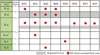
In hydrocarbon exploration, faults can behave as effective conduits for hydrocarbon migration during the short opening episode (Cartwright et al. 1998, Reference Cartwright, Huuse and Aplin2007). The ENE–WSW- to NE–SW-trending major faults cut through the source rock (K₁n₁ mudstone) and the main reservoirs (K₁t, K₁n₁, K₁n₂ and K₁d sandstone) and maintained weak movement during the K₁y–K₂q period. Hence, these two trending major faults could provide vertical conduits during the hydrocarbon charging period (K₁y₂₊₃ period). The activity intensity during episodic movement is one of the reasons for the difference in the vertical distribution of hydrocarbons around different faults (Wang et al. Reference Wang, Chen, Wang, Shi, Xie, Wang, Li and Liao2020). The activity intensity of the NE–SW-trending major faults was obviously stronger than that of the ENE–WSW-trending major faults during the K₁y₂₊₃ period. Moreover, the discovered oil shows that the vertical distribution range of the hydrocarbon accumulation zone around the NE–SW-trending major faults is obviously wider than that of the ENE–WSW-trending major faults (Fig. 12).

Fig. 12.

Wells adjacent to the multi-trending major faults and their corresponding oil shows (locations of wells are shown in Fig. 1d).