





1. Introduction
The addition of dilute polymers to a Newtonian solvent gives rise to a wide variety of complex flow phenomena (Datta et al. Reference Datta2022). The resulting non-Newtonian fluid typically possesses viscoelasticity, an essential rheological property underlying the emergence of diverse behaviours such as rod-climbing (the Weissenberg effect) (Weissenberg Reference Weissenberg1947; Ruangkriengsin et al. Reference Ruangkriengsin, Brandão, Wu, Hwang, Boyko and Stone2025), die swell (Tanner Reference Tanner2005; Tang et al. Reference Tang, Marchesini, Cardon and D’hooge2020), turbulent drag reduction (White & Mungal Reference White and Mungal2008; Graham Reference Graham2014; Choueiri et al. Reference Choueiri, Lopez and Hof2018; Wang et al. Reference Wang, Zhang, Wang, Li, Zhang and Li2023), elastic (Groisman & Steinberg Reference Groisman and Steinberg2000; Steinberg Reference Steinberg2021; Sasmal Reference Sasmal2025) and elastoinertial turbulence (Samanta et al. Reference Samanta, Dubief, Holzner, Schäfer, Morozov, Wagner and Hof2013; Zhang et al. Reference Zhang, Li, Fan, Su, Xi and Sun2025). A particularly significant subset of these phenomena involves the alteration of hydrodynamic stability by polymer-induced stresses. Unlike Newtonian instabilities, which typically stem from inertial effects (Schmid & Henningson Reference Schmid and Henningson2001), polymeric flows are influenced by the interplay between inertia and fluid elasticity, leading to the emergence of elastoinertial instabilities (Dubief et al. Reference Dubief, Terrapon and Hof2023). Remarkably, these flows can also become unstable at vanishing Reynolds number via a pure elastic route (Shaqfeh Reference Shaqfeh1996). The ensuing elastic instability arises when the elasticity-indicating parameter, the Weissenberg (
 $\textit{Wi}$
) number (or Deborah number) – ratio of the polymer relaxation time to the characteristic flow convection time – exceeds a threshold.
Extensive studies have analysed both elastic and elastoinertial instabilities of viscoelastic flows in canonical settings: Taylor–Couette geometry (Muller et al. Reference Muller, Larson and Shaqfeh1989; Larson et al. Reference Larson, Shaqfeh and Muller1990; Shaqfeh et al. Reference Shaqfeh, Muller and Larson1992; Graham Reference Graham1998; Liu & Khomami Reference Liu and Khomami2013; Bai et al. Reference Bai, Latrache, Kelai, Crumeyrolle and Mutabazi2023; Beneitez et al. Reference Beneitez, Mrini and Kerswell2025) and parallel, rectilinear configurations including Kolmogorov (Boffetta et al. Reference Boffetta, Celani, Mazzino, Puliafito and Vergassola2005; Bistagnino et al. Reference Bistagnino, Boffetta, Celani, Mazzino, Puliafito and Vergassola2007; Berti & Boffetta Reference Berti and Boffetta2010; Lewy & Kerswell Reference Lewy and Kerswell2025), planar Couette (Gorodtsov & Leonov Reference Gorodtsov and Leonov1967; Renardy Reference Renardy1992; Morozov & van Saarloos Reference Morozov and van Saarloos2005; Binns & Wynn Reference Binns and Wynn2024), planar Poiseuille (Grosch & Salwen Reference Grosch and Salwen1968; Sureshkumar & Beris Reference Sureshkumar and Beris1995; Wilson et al. Reference Wilson, Renardy and Renardy1999; Khalid et al. Reference Khalid, Chaudhary, Garg, Shankar and Subramanian2021; Lellep et al. 2021) and pipe flows (Garg et al. Reference Garg, Chaudhary, Khalid, Shankar and Subramanian2018; Chaudhary et al. Reference Chaudhary, Garg, Subramanian and Shankar2021; Dong & Zhang Reference Dong and Zhang2022). These geometric configurations admit analytical base-state solutions, which facilitate modal (Renardy & Renardy Reference Renardy and Renardy1986) and non-modal (Jovanović & Kumar Reference Jovanović and Kumar2011) linear stability analyses, as well as weakly nonlinear analyses (Sánchez et al. Reference Sánchez, Jovanović, Kumar, Morozov, Shankar, Subramanian and Wilson2022). These theoretical studies have provided deep insights into the mechanisms of centre-mode instabilities (Garg et al. Reference Garg, Chaudhary, Khalid, Shankar and Subramanian2018), the energy budgets of the eigenmodes (Sadanandan & Sureshkumar Reference Sadanandan and Sureshkumar2004; Hoda et al. Reference Hoda, Jovanović and Kumar2008; Spyridakis et al. Reference Spyridakis, Moschopoulos, Varchanis, Dimakopoulos and Tsamopoulos2024) and the subcritical nature of the transition in shear-dominated parallel flows (Morozov & van Saarloos Reference Morozov and van Saarloos2007; Garg et al. Reference Garg, Chaudhary, Khalid, Shankar and Subramanian2018; Buza et al. Reference Buza, Page and Kerswell2022).
Despite extensive stability analyses of viscoelastic flows with analytical base states, far fewer efforts have addressed those without such base states – typically arising in non-rectilinear geometries. By contrast, a surprisingly large body of experimental and numerical work has reported unstable viscoelastic flows in a broad range of complex geometric domains, including cross-slot (Arratia et al. Reference Arratia, Thomas, Diorio and Gollub2006; Canossi et al. Reference Canossi, Mompean and Berti2020), pore–throat (De et al. Reference De, Kuipers, Peters and Padding2017; Browne et al. Reference Browne, Shih and Datta2020; Ekanem et al. Reference Ekanem, Berg, De, Fadili, Bultreys, Rücker, Southwick, Crawshaw and Luckham2020; Kumar et al. Reference Kumar, Aramideh, Browne, Datta and Ardekani2021), channels with a cylinder (Kenney et al. Reference Kenney, Poper, Chapagain and Christopher2013; Peng et al. Reference Peng, Tang, Li, Zhang and Yu2023) or cylinder arrays (Khomami & Moreno Reference Khomami and Moreno1997; Grilli et al. Reference Grilli, Vázquez-Quesada and Ellero2013; Shi & Christopher Reference Shi and Christopher2016), porous media (Walkama et al. Reference Walkama, Waisbord and Guasto2020; Browne & Datta Reference Browne and Datta2021; Haward et al. Reference Haward, Hopkins and Shen2021; Kumar et al. Reference Kumar, Guasto and Ardekani2022) and so on. This apparent gap between abundant experimental and numerical observations and limited theoretical understanding motivates systematic stability analyses of viscoelastic flows with and without inertia in complex geometries.
Such studies remain scarce, most likely owing to the notorious numerical difficulty of simulating viscoelastic flow, namely the so-called high Weissenberg number problem. To the best of our knowledge, and surprisingly, they have been restricted to global linear stability analyses for two-dimensional (2-D) inertialess flows past a single cylinder (Sureshkumar et al. Reference Sureshkumar, Smith, Armstrong and Brown1999; Smith et al. Reference Smith, Armstrong, Brown and Sureshkumar2000; Spyridakis et al. Reference Spyridakis, Moschopoulos, Varchanis, Dimakopoulos and Tsamopoulos2024) or an array of cylinders (Sureshkumar et al. Reference Sureshkumar, Smith, Armstrong and Brown1999; Smith et al. 2000, 2003; Sahin & Wilson Reference Sahin and Wilson2008) in a channel. Most of these works used the finite element method (FEM) for spatial discretization, whereas Sahin & Wilson (Reference Sahin and Wilson2008) used a finite volume method. These works identified distinct instability mechanisms. Smith et al. (Reference Smith, Armstrong, Brown and Sureshkumar2000) established that flow of an Oldroyd-B fluid past a single cylinder remains linearly stable for all Weissenberg numbers accessible to their analysis, while Spyridakis et al. (Reference Spyridakis, Moschopoulos, Varchanis, Dimakopoulos and Tsamopoulos2024) examined a Phan-Thien–Tanner fluid, identified strain-rate thinning and elasticity as jointly important for the symmetry-breaking bifurcation. For periodic cylinder arrays, the dominant instability arises from perturbations to the shearing velocity-gradient component interacting with base-flow polymeric stresses (Smith et al. Reference Smith, Joo, Armstrong and Brown2003), or from elastic stresses in intercylinder recirculation regions producing spiral vortices (Sahin & Wilson Reference Sahin and Wilson2008). In these configurations, flow instabilities are typically associated with strong shear or curved streamlines, leaving extension-dominated viscoelastic flows in complex geometries largely unexplored.
(a) Schematic of the cross-slot geometry and coordinate system. The domain consists of two opposing horizontal inlets and two opposing vertical outlets, each with a width
 $\tilde {D}$
and length
 $10\tilde {D}$
. The origin
 $O$
is located at the centre, and the flow is divided into four quadrants
 $(\tilde {Q}_1-\tilde {Q}_4)$
. (b) The coarsest mesh, M1, with an inset that highlights the mesh refinement at the central junction.

Figure 1. Long description
Panel A: A schematic of the cross-slot geometry and coordinate system. The domain features two opposing horizontal inlets and two opposing vertical outlets, each with a width and length labeled as D. The origin is marked at the center, and the flow is divided into four quadrants labeled Q1, Q2, Q3, and Q4. Arrows indicate the direction of flow into and out of the inlets and outlets. Panel B: The coarsest mesh, labeled M1, with an inset highlighting the mesh refinement at the central junction. The mesh consists of triangular elements, with a denser concentration of elements near the center to capture detailed flow features.
A representative example is the elastic-instability-induced symmetry breaking of low-Reynolds-number polymeric flows through a nominally symmetric cross-slot microfluidic device. As shown in figure 1(a), it consists of a central square junction connected to four straight side channels arranged orthogonally. Fluid enters through the two opposing horizontal channels and is redirected towards the two vertical outlet branches, producing a stagnation point and an extensional flow downstream of that point. Creeping flow of Newtonian fluids in this device, as expected, preserves the geometric symmetry. By contrast, polymeric flow can break this symmetry through elastic instability: it remains symmetric at low strain rate (low
 $\textit{Wi}$
), transitions to a steady asymmetric state when
 $\textit{Wi}$
exceeds a critical value, and then becomes periodic or even chaotic through a secondary instability as the strain rate, and hence
 $\textit{Wi}$
, increases further. Notwithstanding being first observed nearly half a century ago (Gardner et al. Reference Gardner, Pike, Miles, Keller and Tanaka1982) and later rediscovered and attributed to elastic instability by Arratia et al. (Reference Arratia, Thomas, Diorio and Gollub2006), the mechanism by which elasticity breaks symmetry remains elusive and controversial. Possible mechanisms include compressional flow upstream of the stagnation point (Poole et al. Reference Poole, Alves and Oliveira2007; Rocha et al. Reference Rocha, Poole, Alves and Oliveira2009), extensional flow downstream of it (Cruz et al. Reference Cruz, Poole, Afonso, Pinho, Oliveira and Alves2014), geometrical singularity and strong shear associated with corners (Davoodi et al. 2019, 2021) and the interplay between fluid elasticity and shear-thinning (Yokokoji et al. Reference Yokokoji, Varchanis, Shen and Haward2024).
Using the upper-convected Maxwell model, Poole et al. (Reference Poole, Alves and Oliveira2007) first numerically reproduce steady symmetry breaking in cross-slot viscoelastic flow and attribute the instability to compressional flow upstream of the stagnation point. This view is later indirectly supported by Rocha et al. (Reference Rocha, Poole, Alves and Oliveira2009), who find for finite extendable nonlinear elastic fluids that small corner rounding barely affects the instability onset, thus excluding corner’s geometric singularity as the cause. Cruz et al. (Reference Cruz, Poole, Afonso, Pinho, Oliveira and Alves2014) attribute the steady symmetry breaking to the central extensional flow, which strongly stretches the polymers and generates a birefringent strand with substantial normal stresses and stress gradients. The innovative optimized-shape cross-slot extensional rheometer (OSCER) (Alves Reference Alves2008; Haward et al. Reference Haward, Oliveira, Alves and McKinley2012) eliminates sharp corners and enables the generation of a nearly homogeneous extensional flow. Experiments (Haward & McKinley Reference Haward and McKinley2013; Haward et al. Reference Haward, McKinley and Shen2016) and simulations (Cruz & Alves Reference Cruz and Alves2018) in this configuration nevertheless still reported steady asymmetric flows via instability, thereby excluding corner singularity or near-corner shear as the essential instability driver. Combining experiments and simulations, Davoodi et al. (Reference Davoodi, Domingues and Poole2019) argued that this instability is driven by high streamline curvature and shear rates near corners upon showing the peak values of the Pakdel–McKinley parameter therein. Their placement of a small cylinder at the cross centre indicated minimal impact on the instability, thus excluding the stagnation point as the most critical destabilizing mechanism. Combining experiments on hydrolyzed polyacrylamide solutions and simulations with the linear simplified Phan-Thien–Tanner model, Yokokoji et al. (Reference Yokokoji, Varchanis, Shen and Haward2024) recently proposed that elasticity triggers the cross-slot instability, while shear-thinning helps sustain the resulting steady asymmetric flow. Although these numerical and experimental studies phenomenologically characterize how the instability depends on various aspects of cross-slot flow, they have also led to diverse and sometimes conflicting mechanistic interpretations. A first-principles theoretical prediction of the instability onset and mode structure remains unavailable (Davoodi et al. Reference Davoodi, Houston, Downie, Oliveira and Poole2021), leaving the physical origin of symmetry breaking unresolved nearly half a century after the first experiment (Gardner et al. Reference Gardner, Pike, Miles, Keller and Tanaka1982). This difficulty has been recognized as an open problem in non-Newtonian fluid mechanics (Wilson Reference Wilson2012; Cruz et al. Reference Cruz, Poole, Afonso, Pinho, Oliveira and Alves2014). Indeed, even for this 2-D inertialess flow, Xi & Graham (Reference Xi and Graham2009) described linear stability analysis (LSA) as ‘an exceedingly demanding task’.
In this work, we address this long-standing challenge by integrating global LSA, structural sensitivity and energy-budget analyses, and direct numerical simulations (DNS) for a creeping flow of Oldroyd-B fluid in a standard 2-D cross-slot channel. Through these analyses, we identify the physical mechanism underlying the first symmetry-breaking instability of the cross-slot flow. The paper is organized as follows. We first describe the problem set-up and numerical methods in § 2 and § 3, respectively. After numerically reproducing the classical instability and bifurcation, we present the main results in § 5, including the direct eigenmodes from LSA, the adjoint eigenmodes and wavemaker region from structural sensitivity analysis, and the energy budget. Finally, we summarize our findings and discuss their implications in § 6.
2. Problem formulation
We consider a canonical, 2-D cross-slot flow of polymeric fluids at vanishing Reynolds number. As shown in figure 1, the flow domain comprises a square block of size
 $\tilde {D}$
connected to four side channels of length
 $10\tilde {D}$
; from hereafter,
 $\tilde {(\boldsymbol{\cdot })}$
denotes dimensional variables. Fluid enters the slot through the two horizontal channels, each at an average velocity of
 $\tilde {U}$
, and exits from the two vertical branches. We address the polymeric flow using the incompressible Stokes equations coupled with the diffusive Oldroyd-B constitutive law,
 \begin{align} &\quad \tilde {\boldsymbol{\nabla }} \boldsymbol{\cdot } \tilde {{{\boldsymbol{u}}}} = 0, \\[-12pt]\nonumber \end{align}
 \begin{align} -\tilde {\boldsymbol{\nabla }} \tilde {p} + \mu _s \tilde {\boldsymbol{\nabla }} \boldsymbol{\cdot } &\big [ \tilde {\boldsymbol{\nabla }} \tilde {{{\boldsymbol{u}}}} + \big (\tilde {\boldsymbol{\nabla }} \tilde {{{\boldsymbol{u}}}}\big )^{\textrm {T}} \big ] + \tilde {\boldsymbol{\nabla }} \boldsymbol{\cdot } \tilde {{\boldsymbol{\tau }}} = {\boldsymbol{0}}, \end{align}
where
 $\mu _s$
denotes the solvent viscosity out of the total viscosity
 $\mu$
,
 $\tilde {p}$
and
 $\tilde {{{\boldsymbol{u}}}}$
represent the pressure and fluid velocity, respectively. The polymeric stress tensor
 $\tilde {{\boldsymbol{\tau }}}$
satisfies
 \begin{equation} \tilde {{\boldsymbol{\tau }}} + \lambda \overset {\triangledown }{\tilde {{\boldsymbol{\tau }}}} = \mu _p \big [\tilde {\boldsymbol{\nabla }} \tilde {{{\boldsymbol{u}}}} + \big (\tilde {\boldsymbol{\nabla }} \tilde {{{\boldsymbol{u}}}}\big )^{\textrm {T}}\big ] + \tilde {\epsilon } \tilde {{\nabla} }^2 \tilde {{\boldsymbol{\tau }}}, \end{equation}
where
 $\mu _p = \mu -\mu _s$
is the polymer viscosity,
 $\lambda$
is the relaxation time of polymers,
 $\tilde {\epsilon }$
is the polymer-stress diffusivity and
 $\overset {\triangledown }{\tilde {{\boldsymbol{\tau }}}}$
is the upper-convective derivative of
 $\tilde {{\boldsymbol{\tau }}}$
,
 \begin{equation} \overset {\triangledown }{\tilde {{\boldsymbol{\tau }}}} = \frac {\partial \tilde {{\boldsymbol{\tau }}}}{\partial \tilde {t}} + \tilde {{{\boldsymbol{u}}}} \boldsymbol{\cdot } \tilde {\boldsymbol{\nabla }} \tilde {{\boldsymbol{\tau }}} - \tilde {{\boldsymbol{\tau }}} \boldsymbol{\cdot } \tilde {\boldsymbol{\nabla }} \tilde {{{\boldsymbol{u}}}} - \big(\tilde {\boldsymbol{\nabla }} \tilde {{{\boldsymbol{u}}}}\big)^{\textrm {T}} \boldsymbol{\cdot } \tilde {{\boldsymbol{\tau }}}, \end{equation}
where
 $\tilde {t}$
denotes time.
By choosing
 $\tilde {D}$
,
 $\tilde {U}$
,
 $\tilde {D}/\tilde {U}$
and
 $\mu \tilde {U}/\tilde {D}$
as the characteristic scales of length, velocity, time and pressure/stress, respectively, we derive the dimensionless governing equations,
 \begin{align} \boldsymbol{\nabla } \boldsymbol{\cdot } {{\boldsymbol{u}}} & = 0, \\[-12pt]\nonumber \end{align}
 \begin{align} -\boldsymbol{\nabla }\! p + \beta \boldsymbol{\nabla } \boldsymbol{\cdot } \left [ \boldsymbol{\nabla } {{\boldsymbol{u}}} + \left (\boldsymbol{\nabla } {{\boldsymbol{u}}}\right )^{\textrm {T}} \right ] + \boldsymbol{\nabla } \boldsymbol{\cdot } {\boldsymbol{\tau }} & = {\boldsymbol{0}}, \\[-12pt]\nonumber \end{align}
 \begin{align} {\boldsymbol{\tau }} + \textit{Wi} \left [ \frac {\partial {\boldsymbol{\tau }}}{\partial t} + {{\boldsymbol{u}}} \boldsymbol{\cdot } \boldsymbol{\nabla } {\boldsymbol{\tau }} - {\boldsymbol{\tau }} \boldsymbol{\cdot } \boldsymbol{\nabla } {{\boldsymbol{u}}} - \left (\boldsymbol{\nabla } {{\boldsymbol{u}}}\right )^{\textrm {T}} \boldsymbol{\cdot } {\boldsymbol{\tau }} \right ] & = (1-\beta ) \left [ \boldsymbol{\nabla } {{\boldsymbol{u}}} + \left (\boldsymbol{\nabla } {{\boldsymbol{u}}}\right )^{\textrm {T}} \right ] + \epsilon {\nabla} ^2 {\boldsymbol{\tau }}, \end{align}
where
 $\beta = \mu _s/\mu$
is the ratio of solvent viscosity to the total viscosity,
 $\textit{Wi} = \lambda \tilde {U}/\tilde {D}$
is the Weissenberg number, the ratio of the polymer relaxation time to the characteristic flow convection time and
 $\epsilon = \tilde {\epsilon }/\tilde {D}^2$
denotes the dimensionless diffusivity of polymeric stress. Throughout this study, we set
 $\epsilon = 5 \times 10^{-5}$
in the bulk unless otherwise specified.
At both inlets, we impose the analytical velocity and polymeric stress profiles of a fully developed channel flow of Oldroyd-B fluids (Kundu Reference Kundu1972). At the outlets, zero pressure, zero streamwise velocity gradient and zero transverse velocity component are prescribed. No-slip boundary conditions are applied at all walls. When polymer-stress diffusion is present (
 $\epsilon \gt 0$
) in the bulk, we set
 $\epsilon = 0$
at the walls following Morozov (Reference Morozov2022) and Beneitez et al. (Reference Beneitez, Mrini and Kerswell2025).
3. Numerical methods
We solve (2.4) numerically using FreeFem++ (Hecht Reference Hecht2012), an open-source FEM library. This choice is motivated by our specific emphasis on stability analysis beyond DNS, together with the successful use of FreeFem++ in a broad range of hydrodynamic stability analyses (Sipp & Lebedev Reference Sipp and Lebedev2007; Marquet et al. Reference Marquet, Sipp and Jacquin2008; Fani et al. Reference Fani, Camarri and Salvetti2012; Garnaud et al. Reference Garnaud, Lesshafft, Schmid and Huerre2013; Lashgari et al. Reference Lashgari, Tammisola, Citro, Juniper and Brandt2014; Boujo & Gallaire Reference Boujo and Gallaire2015; Tammisola & Juniper Reference Tammisola and Juniper2016; Fabre et al. Reference Fabre, Citro, Ferreira Sabino, Bonnefis, Sierra, Giannetti and Pigou2018; Douglas & Jolivet Reference Douglas and Jolivet2026).
For numerical stabilization, we adopt the discrete elastic-viscous split-stress gradient (DEVSS-G) formulation (Liu et al. Reference Liu, Bornside, Armstrong and Brown1998) and the streamline upwind Petrov–Galerkin scheme (Baaijens Reference Baaijens1998) as successfully used in our early studies (Zhu et al. 2011, 2012; Su et al. Reference Su, Castillo, Pak, Zhu and Zenit2022; De Corato et al. Reference De Corato, Zhang and Zhu2026), effectively solving the following equations:
 \begin{equation} \boldsymbol{\nabla } \boldsymbol{\cdot } {{\boldsymbol{u}}} =0, \end{equation}
 \begin{equation} {-}\boldsymbol{\nabla }\! p + \boldsymbol{\nabla } \boldsymbol{\cdot } \left [\boldsymbol{\nabla } {{\boldsymbol{u}}} + \left (\boldsymbol{\nabla }{{\boldsymbol{u}}}\right )^{\textrm {T}} \right ] + \boldsymbol{\nabla } \boldsymbol{\cdot } {\boldsymbol{\tau }} + \left (\beta -1\right ) \boldsymbol{\nabla } \boldsymbol{\cdot } \left ( \unicode{x1D642}+ \unicode{x1D642}^{\textrm {T}} \right ) =\boldsymbol{0}, \end{equation}
 \begin{equation} {\boldsymbol{\tau }}+ \textit{Wi} \left ( \frac {\partial {\boldsymbol{\tau }}}{\partial t} + {{\boldsymbol{u}}}\boldsymbol{\cdot }\boldsymbol{\nabla }{\boldsymbol{\tau }} - {\boldsymbol{\tau }}\boldsymbol{\cdot } \unicode{x1D642} - \unicode{x1D642}^{\textrm {T}}\boldsymbol{\cdot }{\boldsymbol{\tau }} \right ) = \left (1-\beta \right ) \left ( \unicode{x1D642}+ \unicode{x1D642}^{\textrm {T}}\right ) + \epsilon {\nabla} ^2 {\boldsymbol{\tau }}, \end{equation}
 \begin{equation} \unicode{x1D642} = \boldsymbol{\nabla } {{\boldsymbol{u}}}, \end{equation}
where
 $ \unicode{x1D642}$
denotes the continuous approximation of the velocity gradient. The computational domain is discretized with triangular Taylor–Hood elements (
 $P2$
–
 $P1$
) for the velocity–pressure pair and piecewise linear continuous elements (
 $P1$
) for
 $\boldsymbol{\tau }$
and
 $ \unicode{x1D642}$
. We solve for
 $p$
,
 ${\boldsymbol{u}}$
and
 $ \unicode{x1D642}$
in a coupled formulation, while addressing the constitutive equation with the characteristic-Galerkin method. Further details of the numerical implementation are provided in Appendix A.
We use three meshes of increasing resolution for the mesh-independence study, which is initiated in the following section § 4 and further detailed in Appendix E. The coarsest mesh M1, presented in figure 1(b), consists of 13 176 elements and 7043 nodes, with element sizes ranging from
 $0.0298$
to
 $0.1414$
. The mesh is locally refined in the central region to better resolve the high polymeric stresses and their sharp gradients expected from the extensional flow therein. Meshes M2 and M3 are generated by successively refining the central region, reducing the minimum element size by a factor of approximately 2.
4. The DNS results on instability and bifurcation
Upon setting the viscosity ratio to
 $\beta = 1/9$
throughout this work (Cruz et al. Reference Cruz, Poole, Afonso, Pinho, Oliveira and Alves2014; Davoodi et al. Reference Davoodi, Domingues and Poole2019, Reference Davoodi, Houston, Downie, Oliveira and Poole2021), we perform time-dependent DNS to reproduce the classical, steady symmetry-breaking instability of viscoelastic cross-slot flow. It is characterized by a transition from a steady symmetric to a steady asymmetric counterpart with increasing
 $\textit{Wi}$
.
Steady flow fields from DNS below and above the symmetry-breaking threshold: (a) stable symmetric state at
 $\textit{Wi}=0.3$
and (b) postbifurcation steady asymmetric state at
 $\textit{Wi}=0.38$
. The fields are visualized by the velocity magnitude
 $|{{\boldsymbol{u}}}|$
with superimposed streamlines. A velocity probe is placed at position
 $A$
to monitor the temporal evolution of the instability in § 4.

(a) Absolute flux imbalance
 $|\Delta Q|$
versus
 $\textit{Wi}$
on meshes M1, M2 and M3, compared with the numerical data of Cruz et al. (Reference Cruz, Poole, Afonso, Pinho, Oliveira and Alves2014). (b) Here
 $( \Delta Q)^2$
versus
 $\textit{Wi}$
; linear extrapolation to zero yields the critical Weissenberg number
 $\textit{Wi}_{cr} = 0.3657$
,
 $0.3630$
and
 $0.3622$
for M1, M2 and M3, respectively.

Figure 2 shows the numerical velocity fields of the stable symmetric state at
 $\textit{Wi}=0.3$
and the postbifurcation asymmetric state at
 $\textit{Wi}=0.38$
, obtained after the simulation reaches a steady regime. At
 $\textit{Wi}=0.3$
, the flow possesses reflection-symmetry about both the horizontal and vertical axes and centrosymmetry about the origin. At
 $\textit{Wi}=0.38$
, the flow presents a skewed pattern, losing both reflection symmetries while retaining centrosymmetry. As documented previously (Arratia et al. Reference Arratia, Thomas, Diorio and Gollub2006; Poole et al. Reference Poole, Alves and Oliveira2007), this flow asymmetry in the cross-slot channel results in an imbalanced distribution of flux within the central junction. Following Rocha et al. (Reference Rocha, Poole, Alves and Oliveira2009) and Cruz et al. (Reference Cruz, Poole, Afonso, Pinho, Oliveira and Alves2014), we quantify this asymmetry using the normalized flux imbalance,
 \begin{equation} \Delta Q = \frac {\left (Q_2+Q_4\right )-\left (Q_1+Q_3\right )}{Q_1+Q_2+Q_3+Q_4}, \end{equation}
where
 $Q_1$
,
 $Q_2$
,
 $Q_3$
and
 $Q_4$
denote the partial fluxes through the four diagonal cross-sections connecting the centre to the corners (see figure 1
a). By definition,
 $\Delta Q=0$
for a symmetric flow given
 $Q_1=Q_2=Q_3=Q_4$
.
We present in figure 3 the absolute flux imbalance
 $|\Delta Q|$
(figure 3
a) and its square
 $( \Delta Q )^2$
(figure 3
b) as functions of
 $\textit{Wi}$
for all three meshes, M1, M2 and M3. The data exhibit a consistent qualitative trend:
 $\Delta Q=0$
remains zero until the onset of instability at a critical Weissenberg number
 $\textit{Wi}_{cr}\approx 0.36$
. Above this threshold,
 $( \Delta Q )^2$
increases linearly with
 $\textit{Wi}-\textit{Wi}_{cr}$
(see figure 3
b), characteristic of the well-recognized supercritical pitchfork bifurcation. Extrapolating the linear fits to
 $( \Delta Q )^2=0$
yields the thresholds,
 $\textit{Wi}_{cr}=0.3657$
,
 $0.3630$
and
 $0.3622$
for M1, M2 and M3, respectively, indicating only weak mesh dependence of
 $\textit{Wi}_{cr}$
. However, an anomalous mesh dependence of
 $|\Delta Q|$
is observed near
 $\textit{Wi}_{cr}$
, which we infer is due to the finite polymer-stress diffusivity
 $\epsilon$
, as discussed in Appendix E. Unless otherwise specified, we use mesh M2 in the remainder of the work.
5. Global linear stability, structural sensitivity and energy–budget analyses
5.1. Global LSA
Having revealed the DNS results, we conduct global LSA to better understand the symmetry-breaking instability. As commonly done, we decompose the state variable
 ${\boldsymbol{q}}({\boldsymbol{x}},t) = [p,{{\boldsymbol{u}}}, \unicode{x1D642}, {\boldsymbol{\tau }}]({\boldsymbol{x}},t)$
into a steady base state
 ${\boldsymbol{q}}^b({\boldsymbol{x}})$
and an infinitesimal perturbation
 ${\boldsymbol{q}}' ({\boldsymbol{x}},t)$
,
 \begin{equation} {\boldsymbol{q}}({\boldsymbol{x}},t) = {\boldsymbol{q}}^b({\boldsymbol{x}}) + {\boldsymbol{q}}'({\boldsymbol{x}},t), \end{equation}
where
 $\boldsymbol{x}$
is the spatial position vector and
 ${\boldsymbol{q}}^b({\boldsymbol{x}})$
is obtained by solving the steady-state governing equations via the Newton–Raphson method, see Appendix B for more details. We linearize the DEVSS-G system (3.1) about the base state and seek perturbations in the normal-mode form
 \begin{equation} {\boldsymbol{q}}'({\boldsymbol{x}},t) = e^{\sigma t} \hat {{\boldsymbol{q}}}({\boldsymbol{x}}), \end{equation}
where
 $\sigma$
is the complex eigenvalue,
 $\hat {{\boldsymbol{q}}}({\boldsymbol{x}})=[\hat {p},\hat {{{\boldsymbol{u}}}}, \hat { \kern-3pt\unicode{x1D642}}, \hat {{\boldsymbol{\tau }}}]({\boldsymbol{x}})$
is the corresponding eigenmode, and
 $\mbox{Re}(\sigma )$
and
 $\mbox{Im}(\sigma )$
denote its temporal growth rate and oscillation frequency, respectively. From hereafter, we refer to
 $\hat {{\boldsymbol{q}}}$
as the direct eigenmode, in contrast to the adjoint eigenmode introduced later in § 5.2. Substituting (5.2) into the linearized perturbation equations yields the direct global stability eigenvalue problem
 \begin{equation} \boldsymbol{\nabla } \boldsymbol{\cdot } \hat {{{\boldsymbol{u}}}} =0, \end{equation}
 \begin{equation} {-}\boldsymbol{\nabla }\! \hat {p} + \boldsymbol{\nabla } \boldsymbol{\cdot } \big [ \boldsymbol{\nabla } \hat {{{\boldsymbol{u}}}} + \big (\boldsymbol{\nabla } \hat {{{\boldsymbol{u}}}}\big )^{\textrm {T}} \big ] + (\beta -1) \boldsymbol{\nabla } \boldsymbol{\cdot } \big (\, \hat { \kern-3pt\unicode{x1D642}} + \hat { \kern-3pt\unicode{x1D642}}^{\textrm {T}} \big ) +\boldsymbol{\nabla } \boldsymbol{\cdot } \hat {{\boldsymbol{\tau }}} ={\boldsymbol{0}}, \end{equation}
 \begin{equation} \hat {{\boldsymbol{\tau }}} + \textit{Wi} \overset {\square }{\hat {{\boldsymbol{\tau }}}} = \left (1-\beta \right ) \big (\,\hat { \kern-3pt\unicode{x1D642}} + \hat { \kern-3pt\unicode{x1D642}}^{\textrm {T}}\big ) + \epsilon {\nabla} ^2 \hat {{\boldsymbol{\tau }}}, \end{equation}
 \begin{equation} \hat { \kern-3pt\unicode{x1D642}} = \boldsymbol{\nabla } \hat {{{\boldsymbol{u}}}}, \end{equation}
where
 $\overset {\square }{\hat {{\boldsymbol{\tau }}}}$
is the linearized upper-convective derivative of
 $\hat {{\boldsymbol{\tau }}}$
,
 \begin{equation} \overset {\square }{\hat {{\boldsymbol{\tau }}}} = \sigma \hat {{\boldsymbol{\tau }}} + {{\boldsymbol{u}}}^{b} \boldsymbol{\cdot } \boldsymbol{\nabla } \hat {{\boldsymbol{\tau }}} + \hat {{{\boldsymbol{u}}}} \boldsymbol{\cdot } \boldsymbol{\nabla } {\boldsymbol{\tau }}^{b} -{\boldsymbol{\tau }}^{b} \boldsymbol{\cdot } \hat { \kern-3pt\unicode{x1D642}} -\hat {{\boldsymbol{\tau }}} \boldsymbol{\cdot } \unicode{x1D642}^{b} -\big ( \unicode{x1D642}^{b}\big )^{\textrm {T}} \boldsymbol{\cdot } \hat {{\boldsymbol{\tau }}} -\hat { \kern-3pt\unicode{x1D642}}^{\textrm {T}} \boldsymbol{\cdot } {\boldsymbol{\tau }}^{b}. \end{equation}
The system (5.3) is subject to the following boundary conditions: zero velocity and stress perturbations at the inlets, vanishing pressure and transverse velocity perturbations at the outlets, and zero velocity perturbation at all walls. Derivation of the eigenvalue problem (5.3) and its numerical implementation are provided in Appendix B.
Using FreeFem++, we solve the discretized form of (5.3) for the complex eigenvalues
 $\sigma$
and the corresponding eigenmodes. Each eigenmode is normalized such that the associated eigenvector of the generalized matrix eigenvalue problem (B4) has unit
 $\ell ^2$
-norm. We then assess the LSA prediction by comparing the real part
 $\sigma _r = \mbox{Re}(\sigma )$
of the leading eigenvalue
 $\sigma$
with the temporal growth rate extracted from DNS. To achieve so, we monitor the time evolution of the
 $x$
-velocity-component,
 $u_A$
, at a probe
 $A: (x,y) = (0,1)$
placed downstream of the stagnation point (see figure 2
b); the magnitude
 $|u_A|$
exhibits an initial exponential growth before saturating at a steady value
 $|u^{ss}_A|$
. Following the Landau amplitude equation (Landau Reference Landau1944; Stuart Reference Stuart1960; Drazin & Reid Reference Drazin and Reid2004), we fit the DNS data through
 \begin{equation} u_A(t) = \frac {u_A^{ss}}{\sqrt {1 + e^{-2\sigma _r(t - t_h)}}}, \end{equation}
treating
 $\sigma _r$
and the half-saturation time
 $t_h$
when
 $u_A = u_A^{ss}/\sqrt {2}$
as fitting parameters. The temporal signals
 $|u_A|(t)$
and their corresponding fitting curves for four unstable
 $\textit{Wi}$
values are depicted in figure 4(a). Its inset further indicates that the data collapse under the rescaling
 \begin{equation} \frac {u_A(T)}{u_A^{ss}} = \frac {1}{\sqrt {1 + e^{-2T}}}, \end{equation}
with
 $T = \sigma _r(t - t_h)$
, supporting a Landau-type amplitude description of the instability growth and saturation.
(a) Time evolution of
 $|u_A|$
at point
 $A: (x,y) = (0,1)$
for
 $\textit{Wi} = 0.37$
,
 $0.38$
,
 $0.39$
and
 $0.40$
; curves show Landau–equation fits. Inset: rescaled velocity
 $u_A/u_A^{ss}$
as a function of the rescaled time
 $T = \sigma _r(t - t_h)$
; data for all
 $\textit{Wi}$
collapse onto the Landau solution
 $1/\sqrt {1+e^{-2T}}$
(solid curve). (b) Leading temporal growth rate
 $\sigma _r$
versus
 $\textit{Wi}$
: LSA results (circles) compared with the DNS counterparts (crosses).

Figure 4(b) illustrates the monotonic increase of the growth rate
 $\sigma _r$
with
 $\textit{Wi}$
, with
 $\sigma _r$
crossing zero at the critical value
 $\textit{Wi}_{cr}$
that marks the onset of instability. For
 $\textit{Wi}\gt \textit{Wi}_{cr}$
, the LSA predictions agree reasonably well with the DNS-derived growth rates, validating our implementation of the eigenvalue problem (5.3). For
 $\textit{Wi}\lt \textit{Wi}_{cr}$
, precise extraction of the decay rate from DNS is difficult, and these values are therefore omitted; this omission does not affect the validation of the LSA implementation. In parallel, the LSA-predicted imaginary part
 $\sigma _i=\mbox{Im}(\sigma )$
of the leading eigenvalue
 $\sigma$
remains negligible across the investigated range of
 $\textit{Wi}$
, consistent with the steady symmetry-breaking character of the pitchfork bifurcation.
Velocity magnitudes with streamlines at
 $\textit{Wi}=0.4$
. (a) The DNS steady asymmetric state
 $|{{\boldsymbol{u}}}|$
; (b) base flow
 $|{{\boldsymbol{u}}}^{b}|$
; (c) leading direct eigenmode
 $|\hat {{{\boldsymbol{u}}}}|$
; (d) and (e) the leading and second DMD modes,
 $|{{\boldsymbol{u}}}_{\boldsymbol{DMD}}^{(1)}|$
and
 $|{{\boldsymbol{u}}}_{\boldsymbol{DMD}}^{(2)}|$
, respectively.

Having verified the growth rate, we now examine the velocity field at
 $\textit{Wi}=0.4$
, starting from the steady-state asymmetric flow field
 $\boldsymbol{u}$
from DNS as displayed in figure 5(a). By symmetry, an equivalent steady state can be obtained by reflecting this field about either the
 $x$
- or
 $y$
-axis, see figure 2(b) for example. Next, the base flow
 ${{\boldsymbol{u}}}^b$
and leading direct eigenmode
 $\hat {{{\boldsymbol{u}}}}$
are shown in figures 5(b) and 5(c), respectively. Beyond DNS and LSA, we further apply dynamic mode decomposition (DMD) (see Appendix B.1) to DNS snapshots from the linear growth regime for a data-driven estimate of the leading continuous-time eigenvalues and associated modes (Rowley et al. Reference Rowley, Mezić, Bagheri, Schlatter and Henningson2009; Schmid Reference Schmid2010). The dominant DMD mode has
 $\omega _{\boldsymbol{DMD}}^{(1)}\approx 0$
and closely reproduces the steady base state (figure 5
b,d). This state stands for the mean flow, exhibiting reflection symmetry across both the horizontal and vertical axes with a central stagnation point and an associated extensional flow.
The next dynamically relevant mode has
 $\mbox{Re}(\omega _{\boldsymbol{DMD}}^{(2)})\approx 0.383$
and
 $\mbox{Im}(\omega _{\boldsymbol{DMD}}^{(2)})\approx 0$
, consistent with the stationary nature of the instability. Its growth rate agrees closely with the DNS estimate
 $\sigma _r\approx 0.373$
and reasonably with the LSA prediction of
 $0.396$
. Notably, its spatial structure matches the leading direct eigenmode from LSA (figure 5
c,e), thereby cross-validating the DNS, LSA and DMD results. This velocity eigenmode forms a diamond-shaped vortical structure with closed streamlines centred at the stagnation point, and its components exhibit the componentwise parity expected for a centred vortex. Such a mode represents a linear signature of the symmetry-breaking mechanism of the viscoelastic cross-slot flow, whereby a chiral velocity perturbation around the stagnation point deflects the separatrices and produces unequal flow partitioning within the two vertical branches.
Polymeric stress components at
 $\textit{Wi}=0.4$
. (a–c) The base state
 $\tau ^{b}_{xx}$
,
 $\tau ^{b}_{xy}$
,
 $\tau ^{b}_{yy}$
; (d–f) leading direct eigenmode
 $\hat {\tau }_{xx}$
,
 $\hat {\tau }_{xy}$
,
 $\hat {\tau }_{yy}$
.

Figure 6. Long description
Panel A: A heatmap shows the base state stress component τ_bxx in a cross-shaped region. The x-axis ranges from -3 to 3, and the y-axis ranges from -3 to 3. The color scale ranges from 0 to 50. Panel B: A heatmap displays the base state stress component τ_bxy in the same region. The x-axis and y-axis ranges are the same as in Panel A. The color scale ranges from -50 to 50. Panel C: A heatmap illustrates the base state stress component τ_byy in the cross-shaped region. The x-axis and y-axis ranges are the same as in Panel A. The color scale ranges from 0 to 200. Panel D: A heatmap shows the leading direct eigenmode stress component τ_xx in the cross-shaped region. The x-axis ranges from -3 to 3, and the y-axis ranges from -3 to 3. The color scale ranges from -2 to 2. Panel E: A heatmap displays the leading direct eigenmode stress component τ_xy in the same region. The x-axis and y-axis ranges are the same as in Panel D. The color scale ranges from -2 to 6. Panel F: A heatmap illustrates the leading direct eigenmode stress component τ_yy in the cross-shaped region. The x-axis and y-axis ranges are the same as in Panel D. The color scale ranges from -0.05 to 0.05.
We then examine the polymeric stress distribution in figure 6, specifically its base state
 ${\boldsymbol{\tau }}^b$
(figure 6
a–c) and leading direct eigenmode
 $\hat {{\boldsymbol{\tau }}}$
(figure 6
d–f). In the base state,
 $\tau _{xx}^{b}$
and
 $\tau _{yy}^{b}$
exhibit double reflection symmetry – being symmetric about both the horizontal and vertical axes – whereas
 $\tau _{xy}^{b}$
exhibits quadrupolar symmetry, being antisymmetric about each axis and invariant under a
 $180^{\circ }$
rotation about the centre. Notably,
 $\tau _{yy}^{b}$
is concentrated along a prominent vertical filament through the cross centre – a birefringent strand associated with strong polymer extension and alignment in the extensional flow downstream of the stagnation point. In contrast, the leading eigenmode displays the opposite parity:
 $\hat {\tau }_{xx}$
and
 $\hat {\tau }_{yy}$
exhibit quadrupolar symmetry, whereas
 $\hat {\tau }_{xy}$
displays double reflection symmetry. This parity reversal suggests that the instability is driven by the antisymmetric normal-stress perturbation
 $\hat {\tau }_{yy}$
that tilts and rotates the birefringent strand. The DNS corroborates this mechanism by capturing the clockwise rotation of the strand (see Appendix F). Considering the vortical velocity perturbation shown in figure 5, the polymer-stress disturbance substantiates the linear signature of the spontaneous symmetry-breaking in the cross-slot flow. Expectedly, the DMD polymeric-stress modes (see Appendix F) mirror the velocity modes: the dominant and second modes recover the base state and the leading direct eigenmode, respectively.
To seek a more intuitional understanding of the polymer microstructural disturbance, we examine the perturbation conformation tensor
 \begin{equation} \hat { \kern-2.5pt \unicode{x1D63E}} = \frac {\textit{Wi}}{1-\beta } \hat {{\boldsymbol{\tau }}}, \end{equation}
which represents the eigenmode of the polymer conformation perturbation corresponding to the leading polymeric-stress eigenmode. It is real and symmetric, therefore admitting the spectral decomposition
 \begin{equation} \hat { \kern-2.5pt \unicode{x1D63E}} = \delta \lambda _1 \,{\boldsymbol{p}}_1{\boldsymbol{p}}_1 + \delta \lambda _2 \,{\boldsymbol{p}}_2 {\boldsymbol{p}}_2, \end{equation}
where
 ${\boldsymbol{p}}_1$
and
 ${\boldsymbol{p}}_2$
denote the orthonormal principal directions of the local polymer-conformation perturbation, and
 $\delta \lambda _i$
(
 $|\delta \lambda _1| \geq |\delta \lambda _2|$
) are the corresponding principal values. Positive and negative
 $\delta \lambda _i$
correspond to stretching and compression perturbations along
 ${\boldsymbol{p}}_i$
, respectively. Inspired by the visualization of Teran et al. (Reference Teran, Fauci and Shelley2010), figure 7 depicts the spatial distribution of
 ${\boldsymbol{p}}_{1,2}$
in the form of two orthogonal segments with lengths proportional to
 $|\delta \lambda _{1,2}|^{1/2}$
. The segments are colour-coded by the sign of
 $\delta \lambda _{1,2}$
– red for positive (stretching) and blue for negative (compression), respectively.
A pair of colour-coded (red or blue) segments at each position indicates principal directions,
 ${\boldsymbol{p}}_1$
and
 ${\boldsymbol{p}}_2$
, of the local polymer-conformation perturbation
 $\hat { \kern-2.5pt \unicode{x1D63E}}$
when
 $\textit{Wi}=0.4$
. The segment lengths are scaled by
 $|\delta \lambda _{1,2}|^{1/2}$
. Red and blue segments denote positive and negative
 $\delta \lambda _{i}$
, respectively, corresponding to stretching and compression perturbations.

This perturbation is weak near the corners (figure 7
c) and does not peak right at the stagnation point. Instead, it is most pronounced along two vertical bands above and below the stagnation point, each resembling a herringbone structure. As shown in figure 7(b) for the upper ‘herringbone’, its left-branch oblique ‘ribs’ represent polymeric compression along an approximate backslash direction, whereas the right-hand counterparts highlight polymeric stretching in an approximate slash direction. This simultaneous side-by-side stretching and compression naturally induces a rotational reorientation of the polymer microstructure along the vertical centreline, thereby triggering the elastic instability. This interpretation is consistent with the rotational perturbation velocity
 $\hat {{{\boldsymbol{u}}}}$
(figure 5
c) and the antisymmetric normal-stress perturbation
 $\hat {\tau }_{yy}$
(figure 6
f).
5.2. Structural sensitivity analysis
While the eigenmodes reveal where the instability is mostly active and hence provide useful insight into the instability mechanism, they cannot pinpoint which regions of the flow are most receptive to external forcing or structural modifications. This complementary information is inherently encoded in the adjoint eigenmode
 $\hat {{\boldsymbol{q}}}^{\dagger }({\boldsymbol{x}}) = [ \hat {p}^{\dagger }, \hat {{{\boldsymbol{u}}}}^{\dagger }, \hat { \kern-3pt\unicode{x1D642}}^{\dagger }, \hat {{\boldsymbol{\tau }}}^{\dagger }]({\boldsymbol{x}})$
. As detailed in Appendix C, we derive the adjoint linearized equation (C9) for the adjoint state variable
 ${\boldsymbol{q}}^\dagger ({\boldsymbol{x}},t) = [ p^{\dagger }, {{\boldsymbol{u}}}^{\dagger }, \unicode{x1D642}^{\dagger }, {\boldsymbol{\tau }}^{\dagger }]({\boldsymbol{x}},t)$
by adapting the framework of Kim (Reference Kim2023), originally developed for drag-sensitivity analysis in viscoelastic flow past a cylinder. Substituting the normal-mode form
 ${\boldsymbol{q}}^{\dagger }({\boldsymbol{x}},t) = e^{-\sigma ^{\dagger } t}\hat {{\boldsymbol{q}}}^{\dagger }({\boldsymbol{x}})$
into (C9) yields the adjoint eigenvalue problem:
 \begin{align} \boldsymbol{\nabla } \boldsymbol{\cdot } \hat {{{\boldsymbol{u}}}}^{\dagger } = 0, \end{align}
 \begin{align} &\boldsymbol{\nabla } \boldsymbol{\cdot } \big [ \boldsymbol{\nabla } \hat {{{\boldsymbol{u}}}}^{\dagger } + \big (\boldsymbol{\nabla } \hat {{{\boldsymbol{u}}}}^{\dagger }\big )^{\textrm {T}} \big ] + (\beta -1)\boldsymbol{\nabla } \boldsymbol{\cdot } \big [\,\hat { \kern-3pt\unicode{x1D642}}^{\dagger }+\big (\hat {\, \kern-3pt\unicode{x1D642}}^{\dagger }\big )^{\textrm {T}}\big ] - \boldsymbol{\nabla }\! \hat {p}^{\dagger } + \textit{Wi} \boldsymbol{\nabla }{\boldsymbol{\tau }}^{b} \, {\boldsymbol{:}}\, \hat {{\boldsymbol{\tau }}}^{\dagger } \nonumber \\ &\quad + 2\textit{Wi}\boldsymbol{\nabla } \boldsymbol{\cdot } \big ({\boldsymbol{\tau }}^{b} \boldsymbol{\cdot } \hat {{\boldsymbol{\tau }}}^{\dagger }\big ) + 2\left (1-\beta \right ) \boldsymbol{\nabla } \boldsymbol{\cdot } \hat {{\boldsymbol{\tau }}}^{\dagger } = {\boldsymbol{0}}, \end{align}
 \begin{align} \hat {{\boldsymbol{\tau }}}^{\dagger } + \textit{Wi}\big [ \sigma ^{\dagger } \hat {{\boldsymbol{\tau }}}^{\dagger } - {{\boldsymbol{u}}}^{b} \boldsymbol{\cdot } \boldsymbol{\nabla }\hat {{\boldsymbol{\tau }}}^{\dagger } - \boldsymbol{\nabla } {{\boldsymbol{u}}}^{b} \boldsymbol{\cdot } \hat {{\boldsymbol{\tau }}}^{\dagger } - \hat {{\boldsymbol{\tau }}}^{\dagger } \boldsymbol{\cdot } \big (\boldsymbol{\nabla } {{\boldsymbol{u}}}^{b}\big )^{\textrm {T}} \big ] - \frac {1}{2}\big [\,\hat { \kern-3pt\unicode{x1D642}}^{\dagger } + \big (\,\hat { \kern-3pt\unicode{x1D642}}^{\dagger }\big )^{\textrm {T}}\big ] - \epsilon {\nabla} ^2 \hat {{\boldsymbol{\tau }}}^{\dagger } = {\boldsymbol{0}}, \end{align}
 \begin{align} \hat { \kern-3pt\unicode{x1D642}}^{\dagger } = \boldsymbol{\nabla } \hat {{{\boldsymbol{u}}}}^{\dagger }. \end{align}
Adjoint eigenmode at
 $\textit{Wi}=0.4$
including its (a–b) velocity components
 $\hat {u}^\dagger$
and
 $\hat {v}^\dagger$
, and (c–e) polymeric-stress components
 $\hat {\tau }_{xx}^\dagger$
,
 $\hat {\tau }_{xy}^\dagger$
and
 $\hat {\tau }_{yy}^\dagger$
.

Figure 8. Long description
Panel A: A heatmap shows the velocity component u† with x and y axes ranging from -3 to 3. The color scale ranges from -4 to 4. Panel B: A heatmap displays the velocity component v† with x and y axes ranging from -3 to 3. The color scale ranges from -1.0 to 1.0. Panel C: A heatmap illustrates the polymeric-stress component τ̂xx with x and y axes ranging from -3 to 3. The color scale ranges from -1.0 to 1.0. Panel D: A heatmap shows the polymeric-stress component τ̂xy with x and y axes ranging from -3 to 3. The color scale ranges from -4 to 2. Panel E: A heatmap displays the polymeric-stress component τ̂yy with x and y axes ranging from -3 to 3. The color scale ranges from -5 to 5.
Equation (5.9) is solved similarly as the eigenvalue problem. The velocity and stress components of the adjoint eigenmode at
 $\textit{Wi} = 0.4$
are presented in figure 8, encoding the spatial distribution of the receptivity of the instability to external forcing. The adjoint velocity components are localized in the central junction region, with
 $\hat {u}^\dagger$
and
 $\hat {v}^\dagger$
being antisymmetric about the horizontal (
 $y=0$
) and vertical (
 $x=0$
) axes, respectively. This spatial distribution indicates that the instability is most receptive to horizontal momentum perturbations downstream of the stagnation point and vertical momentum perturbations upstream of it. For the adjoint stress components,
 $\hat {\tau }_{xx}^\dagger$
is concentrated at the corners with a sign pattern that is antisymmetric about the geometric diagonal, mirroring the structure of the direct eigenmode
 $\hat {\tau }_{xx}$
. The shear component
 $\hat {\tau }_{xy}^\dagger$
fills both inflow arms with positive values while exhibiting a negative region at the central stagnation point and near the corners. Here
 $\hat {\tau }_{yy}^\dagger$
is concentrated near the corners, with an antisymmetric pattern analogous to
 $\hat {\tau }_{xx}^\dagger$
.
The direct and adjoint eigenmodes exhibit markedly different spatial structures, so either mode alone provides limited insight into the instability mechanism. Following Giannetti & Luchini (Reference Giannetti and Luchini2007) and Pralits et al. (Reference Pralits, Brandt and Giannetti2010), we combine the two eigenmodes to define the velocity-based structural sensitivity field,
 \begin{align} \eta _{{{\boldsymbol{u}}}}({\boldsymbol{x}}) = \frac {\left |\hat {{{\boldsymbol{u}}}}({\boldsymbol{x}})\right | \left |\hat {{{\boldsymbol{u}}}}^{\dagger }({\boldsymbol{x}})\right |} {\left |\int _{\varOmega } \hat {{{\boldsymbol{u}}}} \boldsymbol{\cdot } \hat {{{\boldsymbol{u}}}}^{\dagger *}\,\mathrm{d}\varOmega \right |}, \end{align}
which measures the spatial overlap between the direct velocity eigenmode
 $\hat {{{\boldsymbol{u}}}}$
and the adjoint velocity eigenmode
 $\hat {{{\boldsymbol{u}}}}^{\dagger }$
. Here,
 $\varOmega$
denotes the computational domain, and
 $*$
denotes complex conjugation. The classical structural sensitivity analysis, originally developed for inertia-induced instabilities in Newtonian flows, identifies the region where the leading eigenvalue is most sensitive to localized velocity feedback – equivalently – where both the direct and adjoint velocity eigenmodes are large. This region is referred to as the wavemaker often interpreted as the core or origin of instability (Giannetti & Luchini Reference Giannetti and Luchini2007; Luchini & Bottaro Reference Luchini and Bottaro2014; Schmid & Brandt Reference Schmid and Brandt2014), since it marks where the global mode has both strong local amplitude and high receptivity to feedback. For the viscoelastic flow instability considered here, the relevant perturbation dynamics involve not only velocity perturbations but also polymeric stress perturbations. Hence, we introduce an analogous stress structural sensitivity field,
 \begin{align} \eta _{{\boldsymbol{\tau }}}({\boldsymbol{x}}) = \frac {\left |\hat {{\boldsymbol{\tau }}}({\boldsymbol{x}})\right | \left |\hat {{\boldsymbol{\tau }}}^{\dagger }({\boldsymbol{x}})\right |} {\left |\int _{\varOmega } \hat {{\boldsymbol{\tau }}} \, {\boldsymbol{:}}\, \hat {{\boldsymbol{\tau }}}^{\dagger *}\,\mathrm{d}\varOmega \right |}. \end{align}


As shown in figure 9 for
 $\textit{Wi}=0.4$
, the velocity-based sensitivity field
 $\eta _{{{\boldsymbol{u}}}}$
attains large values in two symmetric lobes straddling the
 $y$
-axis, identifying the velocity-based wavemaker region of the instability. Compared with
 $\eta _{{{\boldsymbol{u}}}}$
, the stress-based sensitivity field
 $\eta _{{\boldsymbol{\tau }}}$
is much more strongly localized, indicating that polymeric-stress perturbations play a central role in the elastic instability. The stress-based wavemaker is concentrated along the central, high-strain-rate stripe of the extensional flow: it consists of a pair of vertical filaments located slightly above the stagnation point, together with a reflection-symmetric pair below it. This structure closely resembles the herringbone-like pattern of the concentrated polymer-conformation perturbation shown in figure 7, suggesting that the stress-based wavemaker captures the core of the elastic instability. By contrast, weak sensitivity is observed near the four corners and in the immediate vicinity of the stagnation point, indicating that these regions are less influential in triggering the instability.
(a) Rate of change of the perturbation energy,
 $\mathrm{d} E/\mathrm{d} t$
, and its four energy-budget terms, except
 $\phi _{vis}$
, versus
 $\textit{Wi}$
, see (5.13). (b) Decomposition of the dominant positive energy budget
 $\phi _{\textit{coup}}$
into four components
 $\phi _{\textit{coup}}^{(i)}$
. All quantities have been scaled by
 $|\phi _{vis}|$
. (c) Distribution of the normalized polymeric power density,
 $\mathcal{P}/|\phi _{vis}|$
at
 $\textit{Wi}=0.4$
. Positive values indicate the energetic source that feeds the instability.

Figure 10. Long description
Panel A: A line graph shows the rate of change of perturbation energy and its four energy-budget terms, except one, versus the Weissenberg number. The x-axis is labeled ’Wi’ and ranges from 0.30 to 0.40. The y-axis is labeled with different terms such as φ_p/|φ_vis|, φ_c/|φ_vis|, φ_coup/|φ_vis|, and dE/dt/|φ_vis|. The inset zooms in on the range from 0.30 to 0.40 on the x-axis and -0.02 to 0.02 on the y-axis. Panel B: Another line graph decomposes the dominant positive energy budget into four components, each represented by different line styles. The x-axis is labeled ’Wi’ and ranges from 0.30 to 0.40. The y-axis is labeled with the components φ_coup/|φ_vis|. Panel C: A heatmap shows the distribution of the normalized polymeric power density at a specific Weissenberg number. The x-axis is labeled ’x’ and ranges from -2 to 2. The y-axis is labeled ’y’ and ranges from -1 to 1. The color bar indicates the magnitude of the polymeric power density, with positive values indicating the energetic source that feeds the instability.
5.3. Energy-budget analysis
To identify the energetic origins of the symmetry-breaking instability and further substantiate its physical mechanism, we perform a perturbation energy-budget analysis following Sadanandan & Sureshkumar (Reference Sadanandan and Sureshkumar2004) and Spyridakis et al. (Reference Spyridakis, Moschopoulos, Varchanis, Dimakopoulos and Tsamopoulos2024). By integrating over the domain
 $\varOmega$
, the inner product of the linearized momentum equation with the perturbation velocity
 ${{\boldsymbol{u}}}'$
, we derive the evolution equation for the perturbation energy
 $E$
associated with polymeric stress as detailed in Appendix D:
 \begin{equation} E = \frac {\textit{Wi}}{2} \int _{\varOmega } {{\boldsymbol{u}}}' \boldsymbol{\cdot } \boldsymbol{\nabla } \boldsymbol{\cdot } {\boldsymbol{\tau }}' \mathrm{d} \varOmega . \end{equation}
Strictly speaking,
 $E$
is the perturbation energy per unit out-of-plane length, but is referred to simply as the perturbation energy for brevity throughout this 2-D study. Notably, its rate of change
 $\textrm {d}E/\textrm {d}t$
quantifies whether perturbations are amplified or attenuated: positive rates indicate temporal growth of the perturbation energy and therefore instability. To gain a deeper understanding, we further decompose this instability indicator into four energy-budget terms,
 \begin{equation} \frac {\textrm {d} E}{\textrm {d} t} = \phi _{p} + \phi _{vis} + \phi _{\epsilon } + \phi _{\textit{coup}}, \end{equation}
with each representing the rate of energy production/dissipation rooted in a specific physical mechanism. In particular,
 $\phi _{p}$
is the rate of work done by the perturbation pressure,
 $\phi _{vis}$
represents the viscous dissipation rate that is consistently negative, while
 $\phi _{\epsilon }$
accounts for the energy contribution due to polymer-stress diffusion, with their expressions provided in Appendix D. The remaining term,
 $\phi _{\textit{coup}}$
, standing for the rate of energy exchange arising from the coupling between the base state and the perturbation, is defined as
 \begin{equation} \phi _{\textit{coup}} = -\textit{Wi} \int _{\varOmega } {{\boldsymbol{u}}}'\boldsymbol{\cdot } \boldsymbol{\nabla } \boldsymbol{\cdot } {\boldsymbol{\psi }}' \mathrm{d} \varOmega , \end{equation}
where
 \begin{equation} {\boldsymbol{\psi }}' = {{\boldsymbol{u}}}^{b} \boldsymbol{\cdot } \boldsymbol{\nabla } {\boldsymbol{\tau }}' + {{\boldsymbol{u}}}' \boldsymbol{\cdot } \boldsymbol{\nabla } {\boldsymbol{\tau }}^{b}-{\boldsymbol{\tau }}^{b} \boldsymbol{\cdot } \unicode{x1D642}^{\,\prime}-{\boldsymbol{\tau }}' \boldsymbol{\cdot } \unicode{x1D642}^{b} - \big ( \unicode{x1D642}^{b}\big )^{\textrm {T}} \boldsymbol{\cdot } {\boldsymbol{\tau }}' - (\unicode{x1D642}^{\,\prime })^{\textrm {T}} \boldsymbol{\cdot } {\boldsymbol{\tau }}^{b}. \end{equation}
Figure 10(a) shows the perturbation-energy growth rate
 $\mathrm{d} E/\mathrm{d} t$
and its four energy-budget terms, except
 $\phi _{vis}$
, versus
 $\textit{Wi}$
, where we have normalized all terms by
 $|\phi _{vis}|$
. The net growth rate
 $\textrm {d}E/\textrm {d}t$
becomes positive from negative when
 $\textit{Wi}\gt 0.36$
, consistent with the critical Weissenberg number of the bifurcation identified earlier (see figure 3). Among all the energy-budget terms,
 $\phi _{\textit{coup}}$
is the dominant positive one, and therefore, represents the major energy source. Following Joo & Shaqfeh (Reference Joo and Shaqfeh1992), Shaqfeh (Reference Shaqfeh1996) and Spyridakis et al. (Reference Spyridakis, Moschopoulos, Varchanis, Dimakopoulos and Tsamopoulos2024), we further decompose the coupling term
 $\phi _{\textit{coup}}$
into four parts,
 \begin{equation} \phi _{\textit{coup}} = \sum _{i=1}^{4} \phi _{\textit{coup}}^{(i)}, \end{equation}
as defined in (D7) with corresponding physical interpretations. Figure 10(b) indicates that the dominant contribution to
 $\phi _{\textit{coup}}$
comes from
 $\phi _{\textit{coup}}^{(3)}$
, the coupling between the base-state polymeric stress and the perturbation velocity gradient. As a side note,
 $\phi _{\textit{coup}}^{(1)}$
, representing the coupling between the base-state stress gradient and the perturbation velocity, makes the largest contribution to destabilizing the viscoelastic Dean flow (Joo & Shaqfeh Reference Joo and Shaqfeh1992). However, this term remains negative and thus has a stabilizing effect in the cross-slot flow over the range of
 $\textit{Wi}$
investigated here.
We further extend the domain-integrated energy analysis by investigating the spatial distribution of the energy production rate. First, we rewrite the integrand on the right-hand side of (5.12) as
 \begin{equation} {{\boldsymbol{u}}}' \boldsymbol{\cdot } \boldsymbol{\nabla } \boldsymbol{\cdot } {\boldsymbol{\tau }}' = \boldsymbol{\nabla } \boldsymbol{\cdot } \left ({\boldsymbol{\tau }}' \boldsymbol{\cdot } {{\boldsymbol{u}}}'\right ) - \frac {1}{2}{\boldsymbol{\tau }}' \, {\boldsymbol{:}} \, \left [ \boldsymbol{\nabla } {{\boldsymbol{u}}}' + (\boldsymbol{\nabla } {{\boldsymbol{u}}}')^{\textrm {T}} \right ]\!. \end{equation}
Using the divergence theorem, we obtain
 \begin{equation} \int _{\varOmega } \boldsymbol{\nabla } \boldsymbol{\cdot } \left ({\boldsymbol{\tau }}' \boldsymbol{\cdot } {{\boldsymbol{u}}}'\right ) \mathrm{d}\varOmega = \int _{\partial \varOmega } {\boldsymbol{n}} \boldsymbol{\cdot } {\boldsymbol{\tau }}' \boldsymbol{\cdot } {{\boldsymbol{u}}}' \mathrm{d} \varGamma = 0, \end{equation}
since
 $\hat {{\boldsymbol{\tau }}}\boldsymbol{\cdot }\hat {{{\boldsymbol{u}}}} = {\boldsymbol{0}}$
at all boundaries (as discussed in Appendix D.1). Hence, this integral makes no net contribution to the perturbation energy growth. Then, we focus on the linear growth stage, when the perturbations
 ${{\boldsymbol{u}}}'$
and
 ${\boldsymbol{\tau }}'$
can be represented by the leading normal mode,
 \begin{equation} {{\boldsymbol{u}}}' \sim e^{\sigma _r t} \hat {{{\boldsymbol{u}}}}, \quad {\boldsymbol{\tau }}'\sim e^{\sigma _r t} \hat {{\boldsymbol{\tau }}}, \end{equation}
where
 $\hat {{{\boldsymbol{u}}}}$
and
 $\hat {{\boldsymbol{\tau }}}$
represent the leading direct eigenmodes of the velocity and polymeric stress, respectively. Substituting into the perturbation energy and calculating its derivative leads to
 \begin{equation} \frac {\mathrm{d} E}{\mathrm{d} t} \sim \sigma _r e^{2\sigma _r t} \textit{Wi} \, \int _{\varOmega } \mathcal{P} \mathrm{d} \varOmega , \end{equation}
where
 \begin{equation} \mathcal{P} = - \hat {{\boldsymbol{\tau }}} \, {\boldsymbol{:}} \, \frac { \boldsymbol{\nabla }\hat {{{\boldsymbol{u}}}} + \left (\boldsymbol{\nabla }\hat {{{\boldsymbol{u}}}}\right )^{\textrm {T}} }{2} \end{equation}
denotes the perturbation polymeric power density (per unit volume), which characterizes the local rate of energy exchange between disturbance kinetic energy density (ED) and polymer elastic ED. With this sign convention,
 $\mathcal{P}$
represents the rate at which the disturbance polymeric stress performs work on the disturbance flow. Thus, negative
 $\mathcal{P}$
corresponds to transfer from the kinetic ED of the disturbance fluid motion to the elastic ED stored in deformed polymer chains; whereas positive
 $\mathcal{P}$
indicates the release of stored elastic ED back into the disturbance kinetic ED, which destabilizes the flow.
In the Newtonian limit,
 $\textit{Wi} \to 0$
, the perturbation polymeric stress becomes proportional to, and aligned with, the perturbation strain-rate tensor,
 $\hat {{\boldsymbol{\tau }}} \to (1-\beta ) [\boldsymbol{\nabla }\hat {{{\boldsymbol{u}}}} + (\boldsymbol{\nabla }\hat {{{\boldsymbol{u}}}})^{\textrm {T}}]$
. Consequently,
 $\mathcal{P}$
is proportional to the negative of the disturbance viscous-dissipation density and is therefore non-positive throughout the domain, becoming strictly negative wherever the perturbation strain rate is non-zero. At larger
 $\textit{Wi}$
, the finite polymer relaxation time can introduce a local misalignment, or phase shift, between
 $\hat {{\boldsymbol{\tau }}}$
and
 $\boldsymbol{\nabla }\hat {{{\boldsymbol{u}}}} + (\boldsymbol{\nabla }\hat {{{\boldsymbol{u}}}})^{\textrm {T}}$
. Their inner product may then become negative in localized regions, corresponding to
 $\mathcal{P}\gt 0$
, where stored elastic energy is released back to the disturbance flow and thus promotes instability. As depicted in figure 10(c), the polymeric power density
 $\mathcal{P}$
attains its largest positive values along a vertical ridge aligning with the central zone of the extensional flows downstream of the stagnation point. This region marks the energetic source of the instability. Importantly, this ridge closely matches the stress-based wavemaker shown in figure 9(b), hence confirming the spatial origin of the elastic instability.
Normalized perturbation polymeric power density,
 $\mathcal{P}/|\phi _{vis}|$
, in cross-slot devices with (a) rounded corners of arc radius
 $0.05$
and (b) a centred cylinder of diameter
 $0.25$
. Here,
 $\textit{Wi}=0.4$
and
 $\epsilon =5\times 10^{-5}$
.

We conclude the energy-budget analysis by examining two geometric variants of the baseline cross-slot setting – rounded corners and a centred cylinder – to further elucidate the instability mechanism. Specifically, the first variant adopts rounded corners with an arc radius of
 $0.05$
, removing the geometric singularities of sharp corners and resulting stress singularities. The second variant introduces a circular cylinder of diameter
 $0.25$
at the centre, thereby eliminating the original free stagnation point. We perform LSA and energy-budget analysis, with the direct eigenmodes presented in Appendix F. Figure 11 shows the distribution of the polymeric power density
 $\mathcal{P}$
. Similar to the baseline setting, the instability persists and the density
 $\mathcal{P}$
remains strongly localized along vertical ridges lying within the central zone of the extensional flows downstream of the stagnation point or of the cylinder. This similarity indicates that strong extensional flows and the ensuing polymer stretching rather than the corner singularity or the central stagnation point, constitute the essential ingredient of the elastic instability in cross-slot devices. Hence, this understanding justifies the persistence of symmetry-breaking instability of viscoelastic flows through the OSCER variant of cross-slot channel that features smooth corners and a nearly homogeneous extensional flow (Haward & McKinley Reference Haward and McKinley2013; Haward et al. Reference Haward, McKinley and Shen2016; Cruz & Alves Reference Cruz and Alves2018). It also explains why the onset of instability remains barely changed when the stagnation point is eliminated by inserting a small cylinder there (Davoodi et al. Reference Davoodi, Domingues and Poole2019): the extensional flows downstream of the cylinder, together with the associated birefringent strand and phase-delay-induced positive polymeric power density, persist despite the absence of the free stagnation point. We further analyse the dominant energy-production term
 $\phi _{\textit{coup}}$
. Following a procedure similar to the derivation of (5.20), we rewrite (5.14), the definition of
 $\phi _{\textit{coup}}$
, in the following modal form:
 \begin{equation} \phi _{\textit{coup}} \sim e^{2\sigma _r t} \textit{Wi} \int_ \varOmega \hat {{\boldsymbol{\psi }}} : \boldsymbol{\nabla } \hat {{{\boldsymbol{u}}}} \mathrm{d} , \end{equation}
where
 $\hat {{\boldsymbol{\psi }}}$
is the modal form of
 ${\boldsymbol{\psi }}^{\prime }$
defined in (5.15),
 \begin{equation} \hat {{\boldsymbol{\psi }}} = {{\boldsymbol{u}}}^{b} \boldsymbol{\cdot } \boldsymbol{\nabla } \hat {{\boldsymbol{\tau }}} + \hat {{{\boldsymbol{u}}}} \boldsymbol{\cdot } \boldsymbol{\nabla } {\boldsymbol{\tau }}^{b} - {\boldsymbol{\tau }}^{b} \boldsymbol{\cdot } \hat { \kern-3pt\unicode{x1D642}} - \hat {{\boldsymbol{\tau }}} \boldsymbol{\cdot } \unicode{x1D642}^{b} - \big( \unicode{x1D642}^{b}\big)^{\textrm {T}} \boldsymbol{\cdot } \hat {{\boldsymbol{\tau }}} - \big( \hat { \kern-3pt\unicode{x1D642}}\big)^{\textrm {T}} \boldsymbol{\cdot } {\boldsymbol{\tau }}^{b}. \end{equation}
The spatial distribution of the integrand (
 $\hat {{\boldsymbol{\psi }}}:\boldsymbol{\nabla } \hat {{{\boldsymbol{u}}}}$
) is plotted in Appendix F. For all three geometries, the spatial distribution exhibits a localized pattern aligned with the birefringent strand, similar to that of the polymeric power density. This similarity further supports the role of the identified energetic `hotspot’ in feeding the instability.
6. Conclusion and discussion
In this work, we revisit the stability of 2-D creeping viscoelastic flow in a cross-slot channel to clarify the mechanism underlying its first, steady symmetry-breaking instability. Although this instability was first observed experimentally nearly half a century ago (Gardner et al. Reference Gardner, Pike, Miles, Keller and Tanaka1982) and reproduced numerically nearly two decades ago (Poole et al. Reference Poole, Alves and Oliveira2007), its physical origin remains debated. To address this long-standing issue, we study inertialess cross-slot flow of a diffusive Oldroyd-B fluid by combining DNS, global LSA, structural sensitivity analysis and energy-budget analysis, all implemented within the FEM library FreeFem++.
Our DNS captures the canonical symmetric-to-asymmetric flow transition through a pitchfork bifurcation at
 $\textit{Wi}_{cr} \approx 0.36$
. The LSA gives a consistent prediction of the critical Weissenberg number and of the temporal growth rates obtained from DNS. Moreover, the base state used in LSA and the leading direct eigenmode are recovered by the dominant zero-frequency and second DMD modes, respectively. These results collectively provide a stringent validation of our LSA implementation.
The leading velocity eigenmode from the LSA forms a centred, diamond-shaped vortical structure with closed streamlines, while the corresponding normal-polymeric-stress eigenmode exhibits antisymmetric parity. Together, they constitute a chiral linear perturbation that drives spontaneous symmetry breaking in the viscoelastic cross-slot flow by tilting and rotating the birefringent strand generated by the vertically oriented extensional flows. This mechanistic picture is further highlighted by visualizing the perturbation conformation tensor via spectral decomposition.
Beyond DNS and LSA, structural sensitivity analysis reveals a stress-based wavemaker region that marks the spatial core of the instability. This region, where the flow is highly sensitive to localized polymeric-stress perturbations, lies with the extensional-flow core and comprises vertical filaments arranged symmetrically about the stagnation point. This spatial configuration coincides with regions of strong perturbation conformation, naturally linking the wavemaker to the polymer-stretching/compression response.
We examine the growth of perturbation energy through a decomposition into four energy-budget contributions, each rooted in a distinct physical mechanism. The dominant contribution comes from the coupling between the base state and the perturbation fields, primarily between the base-state polymeric stress and the perturbation velocity gradient. It can be further characterized by the disturbance polymeric power density
 $\mathcal{P}$
measuring the rate at which the disturbance polymeric stress performs work on the disturbance flow. Notably, positive
 $\mathcal{P}$
is most pronounced in a vertical ridge along the centreline extensional flows downstream of the stagnation point, identifying the energetic source of the elastic instability. Its spatial overlap with the stress-based wavemaker further establishes this narrow, extension-dominated zone as the instability core. We further test this insight by studying two geometric variants of the baseline setting: a cross-slot channel with rounded corners and another containing a centred cylinder eliminating the stagnation point. In both cases, peak power density
 $\mathcal{P}$
appears along vertical ridges aligned with the central high-extension-rate zones, reinforcing the proposed instability mechanism. Recent experiments combining synchronized polarization imaging and particle tracking (Salipante et al. Reference Salipante, Cromer, Pradillo and Hudson2025) offer a potential route to reconstruct the polymeric-stress field and test the mechanism experimentally.
These findings help reconcile the debate over whether the instability originates from sharp corners or from the stagnation point. Studies on the OSCER variant of the cross-slot channel (Haward & McKinley Reference Haward and McKinley2013; Haward et al. Reference Haward, McKinley and Shen2016; Cruz & Alves Reference Cruz and Alves2018) suggest that sharp corners are not necessary for the instability, whereas the cylinder-inserted, stagnation-point-free set-up investigated in Davoodi et al. (Reference Davoodi, Domingues and Poole2019) points instead to corner-induced streamline curvature and high deformation rates. We find that neither the corner nor the free central stagnation point is the essential ingredient; rather, the spatial core of the instability lies in narrow high-extension-rate regions within the extensional flows. This explanation is more consistent with the instability mechanism of ‘large normal stresses and gradients in the birefringence strand’ in extensional flow proposed by Cruz et al. (Reference Cruz, Poole, Afonso, Pinho, Oliveira and Alves2014). As a side note, we find no evidence that upstream compressional-flow disturbances are relevant to the instability onset, contrary to earlier hypotheses. Further, we notice that our analysis is qualitatively compatible with the interpretation of the OSCER instability in terms of the coupling between streamline curvature and streamwise elastic tensile stress, as characterized by the Pakdel–McKinley criterion (Haward et al. Reference Haward, McKinley and Shen2016). The corresponding parameter peaks near the central stagnation point, close to the downstream extensional ‘hotspot’ identified here.
In summary, our results offer insights into the long-standing controversy over the physical origin of the creeping viscoelastic-flow instability in the cross-slot channel. More broadly, this study demonstrates the potential of integrating global stability, structural sensitivity and energy-budget analyses to understand instability in viscoelastic flows through complex geometries for which analytical base states are unavailable. Future work will extend the current framework to systematically investigate related viscoelastic flow instabilities involving other ingredients, including three-dimensional perturbations and flows, other complex geometries, finite inertia, realistic rheological models, unsteady base states, capillary interfaces and deformable structures.
Acknowledgements
The authors thank J. Kim, A. Spyridakis and D. Wan for useful discussions.
Funding
L.Z. acknowledges the support from the Singapore Ministry of Education Academic Research Fund Tier 2 (MOE-T2EP50122-0015) and Tier 1 grants (A-8003190-00-00). Computation of the work was performed on resources of the National Supercomputing Centre, Singapore (https://www.nscc.sg), as well as those provided by NUS IT via a grant (NUSREC-HPC-00001).
Declaration of interests
The authors report no conflict of interest.
Data availability statement
The source code used in this study is publicly available at https://github.com/LailaiGroup/FreeFEM-solvers-for-creeping-Oldroyd-B-cross-slot-flow.
Appendix A. Numerical methods for DNS
Here, we describe the FEM formulation and the time-advancement scheme used for the DNS. We first derive the weak form of the DEVSS-G formulation (3.1). We use
 $\breve {(\boldsymbol{\cdot })}$
to denote the test functions for the corresponding variables. Multiplying the momentum equation (3.1b) by the velocity test function
 $\breve {{{\boldsymbol{u}}}} = ( \breve {u}, \breve {v})$
, integrating over the domain
 $\varOmega$
and applying integration by parts to the pressure and viscous-stress terms gives
 \begin{eqnarray} & &\int _{\varOmega } \left \{ - p \boldsymbol{\nabla } \boldsymbol{\cdot } \breve {{{\boldsymbol{u}}}} + \boldsymbol{\nabla } \breve {{{\boldsymbol{u}}}} \, {\boldsymbol{:}} \, \left [\boldsymbol{\nabla }{{\boldsymbol{u}}}+ \left (\boldsymbol{\nabla } {{\boldsymbol{u}}}\right )^{\textrm {T}} \right ] -\breve {{{\boldsymbol{u}}}} \boldsymbol{\cdot } \boldsymbol{\nabla } \boldsymbol{\cdot } {\boldsymbol{\tau }} + \breve {{{\boldsymbol{u}}}} \boldsymbol{\cdot } \left [ \left (1-\beta \right )\boldsymbol{\nabla } \boldsymbol{\cdot } \left ( \unicode{x1D642}+ \unicode{x1D642}^{\textrm {T}}\right )\right ] \right \} \mathrm{d}\varOmega \nonumber \\& & \qquad +\int _{\partial \varOmega } \breve {{{\boldsymbol{u}}}} \boldsymbol{\cdot } \left \{ {\boldsymbol{n}} \boldsymbol{\cdot } \left [ p \unicode{x1D644}- [\boldsymbol{\nabla } {{\boldsymbol{u}}}+\left (\boldsymbol{\nabla } {{\boldsymbol{u}}}\right )^{\textrm {T}}] \right ] \right \} \mathrm{d} \varGamma = 0, \end{eqnarray}
where
 $\varOmega$
denotes the computational domain,
 $\partial \varOmega$
denotes its boundary,
 $\mathrm{d}\varOmega$
is the area element in
 $\varOmega$
,
 $\mathrm{d}\varGamma$
is the line element on
 $\partial \varOmega$
and
 ${\boldsymbol{n}} = (n_x,n_y)$
denotes the unit normal on
 $\partial \varOmega$
, pointing from the fluid towards the exterior.
The boundary term vanishes on the walls and inlet, where Dirichlet conditions are imposed on the velocity and the corresponding velocity test function is zero. We consider a fully developed flow for the outlet boundary. For the upper outlet in the cross-slot,
 $u=0, p=0$
and
 $({\partial v}/{\partial y})=0$
. Then the integral on the outlet boundary becomes
 \begin{equation} \int _{\partial \varOmega } \breve {{{\boldsymbol{u}}}} \boldsymbol{\cdot } \left \{ {\boldsymbol{n}} \boldsymbol{\cdot } \left [p \unicode{x1D644}- [\boldsymbol{\nabla } {{\boldsymbol{u}}}+\left (\boldsymbol{\nabla } {{\boldsymbol{u}}}\right )^{\textrm {T}}]\right ]\right \} \mathrm{d} \varGamma = -\int _{\partial \varOmega } \breve {{{\boldsymbol{u}}}} \boldsymbol{\cdot } \left \{ {\boldsymbol{n}} \boldsymbol{\cdot } \left [\boldsymbol{\nabla } {{\boldsymbol{u}}}+\left (\boldsymbol{\nabla } {{\boldsymbol{u}}}\right )^{\textrm {T}}\right ]\right \} \mathrm{d} \varGamma . \end{equation}
For the upper outlet boundary featuring
 $n_x=0, n_y=1$
, we apply the boundary condition
 $u=0$
and hence its associated test function
 $\breve {u}=0$
. Then the boundary term there vanishes,
 \begin{equation} -\breve {{{\boldsymbol{u}}}} \boldsymbol{\cdot } \left \{ {\boldsymbol{n}} \boldsymbol{\cdot } \left [\boldsymbol{\nabla } {{\boldsymbol{u}}}+\left (\boldsymbol{\nabla } {{\boldsymbol{u}}}\right )^{\textrm {T}} \right ]\right \} = -\breve {u}_{\kappa } n_{\zeta } \left (\frac {\partial u_{\kappa }}{\partial x_{\zeta }} + \frac {\partial u_{\zeta }}{\partial x_{\kappa }}\right ) = -2 \breve {v} \frac {\partial v}{\partial y} = 0. \end{equation}
So as it does at the lower outlet.
The weak form of the velocity gradient approximation
 $ \unicode{x1D642} = \boldsymbol{\nabla } {{\boldsymbol{u}}}$
is
 \begin{equation} \int _{\varOmega } \breve { \unicode{x1D642}} \, {\boldsymbol{:}} \, \left ( \unicode{x1D642} - \boldsymbol{\nabla } {{\boldsymbol{u}}}\right ) \mathrm{d}\varOmega =0. \end{equation}
The weak form of the continuity equation is
 \begin{equation} \int _{\varOmega } {\breve {p}} \boldsymbol{\nabla } \boldsymbol{\cdot } {{\boldsymbol{u}}} \mathrm{d}\varOmega = 0. \end{equation}
The weak form of the constitutive equation is
 \begin{eqnarray} && \int _{\varOmega } \breve {{\boldsymbol{\tau }}} \, {\boldsymbol{:}} \, \left [{\boldsymbol{\tau }} +\textit{Wi}\left (\frac {\partial {\boldsymbol{\tau }}}{\partial t} + {{\boldsymbol{u}}} \boldsymbol{\cdot } \boldsymbol{\nabla } {\boldsymbol{\tau }} -{\boldsymbol{\tau }} \boldsymbol{\cdot } \unicode{x1D642} - \unicode{x1D642}^{\textrm {T}} \boldsymbol{\cdot } {\boldsymbol{\tau }} \right ) + \left (\beta -1\right ) \left ( \unicode{x1D642}+ \unicode{x1D642}^{\textrm {T}} \right )\right ] +\epsilon \boldsymbol{\nabla } \breve {{\boldsymbol{\tau }}} \, {\boldsymbol{:}} \, \boldsymbol{\nabla } {\boldsymbol{\tau }} \mathrm{d}\varOmega \nonumber \\ &&\quad - \epsilon \int _{\partial \varOmega } {\boldsymbol{n}} \boldsymbol{\cdot } \left (\boldsymbol{\nabla } {\boldsymbol{\tau }} \, {\boldsymbol{:}} \, \breve {{\boldsymbol{\tau }}}\right ) \, \mathrm{d} \varGamma =0. \end{eqnarray}
We first note that the boundary integral involving stress diffusion in (A6) vanishes on each part of
 $\partial \varOmega$
. At the walls, we have set
 $\epsilon = 0$
following Beneitez et al. (Reference Beneitez, Mrini and Kerswell2025), leading to zero integral. At the inlets, we impose the analytical polymeric stress profile as Dirichlet boundary conditions, so the test function
 $\breve {{\boldsymbol{\tau }}} = {\boldsymbol{0}}$
, again rendering the integral zero. At the outlets, the natural boundary condition of the weak formulation implicitly enforces
 ${\boldsymbol{n}} \boldsymbol{\cdot } \boldsymbol{\nabla }{\boldsymbol{\tau }} = {\boldsymbol{0}}$
, so that
 \begin{align} -\epsilon \int _{\partial \varOmega } {\boldsymbol{n}} \boldsymbol{\cdot } \left (\boldsymbol{\nabla }{\boldsymbol{\tau }} \, {\boldsymbol{:}} \, \breve {{\boldsymbol{\tau }}}\right )\,\mathrm{d} \varGamma = -\epsilon \int _{\partial \varOmega } \left ({\boldsymbol{n}} \boldsymbol{\cdot } \boldsymbol{\nabla }{\boldsymbol{\tau }}\right )\, {\boldsymbol{:}} \, \breve {{\boldsymbol{\tau }}}\,\mathrm{d} \varGamma = 0. \end{align}
As the boundary contribution vanishes entirely, we obtain the following weak form of the constitutive equation:
 \begin{align} \int _{\varOmega } \left \{ \breve {{\boldsymbol{\tau }}} \, {\boldsymbol{:}} \, \left [ {\boldsymbol{\tau }} + \textit{Wi}\left (\frac {\partial {\boldsymbol{\tau }}}{\partial t} + {{\boldsymbol{u}}} \boldsymbol{\cdot } \boldsymbol{\nabla } {\boldsymbol{\tau }} - {\boldsymbol{\tau }} \boldsymbol{\cdot } \unicode{x1D642} - \unicode{x1D642}^{\textrm {T}} \boldsymbol{\cdot } {\boldsymbol{\tau }} \right ) + (\beta -1 )\big ( \unicode{x1D642}+ \unicode{x1D642}^{\textrm {T}} \big ) \right ] +\epsilon \boldsymbol{\nabla } \breve {{\boldsymbol{\tau }}} : \boldsymbol{\nabla } {\boldsymbol{\tau }} \right \} \mathrm{d}\varOmega = 0. \end{align}
For unsteady DNS, we advance the solution from time level
 $t_n$
at step
 $n$
to
 $t_{n+1}$
at step
 $n+1$
, where
 $\Delta t = t_{n+1}-t_n$
denotes the step size. We employ a decoupled time stepping scheme consisting of two substeps. In the first substep, given the stress field
 ${\boldsymbol{\tau }}_n$
at time level
 $t_n$
, we solve a coupled system comprising the continuity equation, the momentum equation and the auxiliary equation for the velocity-gradient tensor to obtain
 $p_{n+1}$
,
 ${{\boldsymbol{u}}}_{n+1}$
and
 $ \unicode{x1D642}_{n+1}$
:
 \begin{align} &\int _{\varOmega } \Big \{{-} p_{n+1} \boldsymbol{\nabla } \boldsymbol{\cdot } \breve {{{\boldsymbol{u}}}} + \boldsymbol{\nabla } \breve {{{\boldsymbol{u}}}} \, {\boldsymbol{:}} \, \big [\boldsymbol{\nabla } {{\boldsymbol{u}}}_{n+1}+ \big ( \boldsymbol{\nabla } {{\boldsymbol{u}}}_{n+1}\big )^{\textrm {T}} \big ] -\breve {{{\boldsymbol{u}}}} \boldsymbol{\cdot } \boldsymbol{\nabla } \boldsymbol{\cdot } {\boldsymbol{\tau }}_n + \breve {{{\boldsymbol{u}}}} \boldsymbol{\cdot } \big [ (1-\beta)\boldsymbol{\nabla } \boldsymbol{\cdot } \big ( \unicode{x1D642}_{n+1}+ \unicode{x1D642}_{n+1}^{\textrm {T}}\big )\big ] \nonumber \\ & \quad -{\breve {p}} \boldsymbol{\nabla } \boldsymbol{\cdot } {{\boldsymbol{u}}}_{n+1} +\breve { \unicode{x1D642}} \, {\boldsymbol{:}} \, \big ( \unicode{x1D642}_{n+1} -\boldsymbol{\nabla } {{\boldsymbol{u}}}_{n+1}\big ) \Big \} \mathrm{d}\varOmega = 0. \end{align}
In the second substep, the constitutive equation is solved to update
 ${\boldsymbol{\tau }}_{n+1}$
by a characteristic-Galerkin method (Pironneau Reference Pironneau1982; Machmoum & Esselaoui Reference Machmoum and Esselaoui2001; Lukáčová-Medvid’ová et al. Reference Lukáčová-Medvid’ová, Notsu and She2016), namely,
 \begin{eqnarray} &&\int _{\varOmega } \Bigl \{ \breve {{\boldsymbol{\tau }}} \, {\boldsymbol{:}} \, \left [{\boldsymbol{\tau }}_{n+1} + \textit{Wi}\left ( \frac {{\boldsymbol{\tau }}_{n+1}-{\boldsymbol{\tau }}_n \circ {\boldsymbol{X}}_n(t_n)}{\Delta t} - {\boldsymbol{\tau }}_{n+1} \boldsymbol{\cdot } \unicode{x1D642}_{n+1} - \unicode{x1D642}_{n+1}^{\textrm {T}} \boldsymbol{\cdot } {\boldsymbol{\tau }}_{n+1} \right ) \right . \nonumber \\ && \left . \quad +\left (\beta -1\right )\left ( \unicode{x1D642}_{n+1}+ \unicode{x1D642}_{n+1}^{\textrm {T}}\right ) \right ] +\epsilon \boldsymbol{\nabla } \breve {{\boldsymbol{\tau }}} \, {\boldsymbol{:}} \, \boldsymbol{\nabla } {\boldsymbol{\tau }}_{n+1} \Bigr \} \mathrm{d}\varOmega = 0, \end{eqnarray}
where
 ${\boldsymbol{X}}_n$
denotes the trajectory (or characteristics) of a fluid particle. Here,
 ${\boldsymbol{X}}_n(t,{\boldsymbol{x}})$
is obtained by solving
 \begin{equation} \begin{cases} \frac {\mathrm{d}}{\mathrm{d} t} {\boldsymbol{X}}_n \left (t,{\boldsymbol{x}}\right ) = {{\boldsymbol{u}}}_{n}\bigl ({\boldsymbol{X}}_n(t,{\boldsymbol{x}})\bigr ), \quad t\in [t_n,t_{n+1}], \\[11pt] {\boldsymbol{X}}_n\left (t_{n+1},{\boldsymbol{x}}\right ) = {\boldsymbol{x}}. \end{cases} \end{equation}
Approximating this trajectory by a first-order scheme gives the upwind point
 ${\boldsymbol{X}}_n(t_n,{\boldsymbol{x}}) \approx {\boldsymbol{x}}-{{\boldsymbol{u}}}_n({\boldsymbol{x}})\,\Delta t$
. Thus, the composition term is written as
 ${\boldsymbol{\tau }}_n\circ {\boldsymbol{X}}_n(t_n,{\boldsymbol{x}})={\boldsymbol{\tau }}_n ({\boldsymbol{X}}_n(t_n, {\boldsymbol{x}}))$
, which is the previous-step stress evaluated at the upwind point.
Finally, we spatially discretize the weak forms using the finite-element spaces introduced in § 3: triangular Taylor–Hood elements (
 $P_2$
–
 $P_1$
) for the velocity–pressure pair and continuous piecewise-linear elements (
 $P_1$
) for
 $\boldsymbol{\tau }$
and
 $ \unicode{x1D642}$
. We then assemble and solve the resulting discrete systems in FreeFem++. Within this discrete setting, we further stabilize the stress update with a streamline upwind Petrov–Galerkin scheme (Baaijens Reference Baaijens1998), replacing the stress test function
 $\breve {{\boldsymbol{\tau }}}$
by
 \begin{equation} \breve {{\boldsymbol{\tau }}}_{\textit{SUPG}}=\breve {{\boldsymbol{\tau }}}+\alpha \, {{\boldsymbol{u}}} \boldsymbol{\cdot } \boldsymbol{\nabla } \breve {{\boldsymbol{\tau }}}, \end{equation}
where
 $\alpha =c_s h/|{{\boldsymbol{u}}}|$
,
 $h$
is the characteristic element size and
 $c_s=0.3$
is a tuneable constant.
Appendix B. Global LSA: derivation and implementation
Here, we detail the derivation for the global LSA and describe the associated numerical implementation. We begin with the base state, whose governing equations are obtained by dropping the temporal derivative of (3.1):
 \begin{align} \boldsymbol{\nabla } \boldsymbol{\cdot } {{\boldsymbol{u}}}^{b}=0, \\[-28pt] \nonumber \end{align}
 \begin{align}\boldsymbol{\nabla }\! p^{b} -\boldsymbol{\nabla } \boldsymbol{\cdot } \big [ \boldsymbol{\nabla } {{\boldsymbol{u}}}^{b} + \big (\boldsymbol{\nabla } {{\boldsymbol{u}}}^{b}\big )^{\textrm {T}} \big ] -\boldsymbol{\nabla } \boldsymbol{\cdot } {\boldsymbol{\tau }}^{b} + (1-\beta ) \boldsymbol{\nabla } \boldsymbol{\cdot }\big [ \unicode{x1D642}^{b} + \big( \unicode{x1D642}^{b}\big)^{\textrm {T}}\big ] ={\boldsymbol{0}}, \\[-28pt] \nonumber \end{align}
 \begin{align}{\boldsymbol{\tau }}^{b} + \textit{Wi}\big [ {{\boldsymbol{u}}}^{b} \boldsymbol{\cdot } \boldsymbol{\nabla } {\boldsymbol{\tau }}^{b} - {\boldsymbol{\tau }}^{b} \boldsymbol{\cdot } \unicode{x1D642}^{b} - \big ( \unicode{x1D642}^{b} \big )^{\textrm {T}} \boldsymbol{\cdot } {\boldsymbol{\tau }}^{b} \big ] = (1-\beta )\big [ \unicode{x1D642}^{b} + \big( \unicode{x1D642}^{b}\big)^{\textrm {T}}\big ] + \epsilon {\nabla} ^2 {\boldsymbol{\tau }}^{b}, \\[-28pt] \nonumber \end{align}
 \begin{align} \unicode{x1D642}^{b}=\boldsymbol{\nabla } {{\boldsymbol{u}}}^{b}. \\[-12pt] \nonumber \end{align}
Subtracting equation (B1) from (3.1), we obtain the perturbation equation:
 \begin{align} \boldsymbol{\nabla } \boldsymbol{\cdot } {{\boldsymbol{u}}}^{\prime }=0, \\[-28pt] \nonumber \end{align}
 \begin{align} \boldsymbol{\nabla }\! p^{\prime } -\boldsymbol{\nabla } \boldsymbol{\cdot } \big [ \boldsymbol{\nabla } {{\boldsymbol{u}}}^{\prime } + \big (\boldsymbol{\nabla } {{\boldsymbol{u}}}^{\prime }\big )^{\textrm {T}} \big ] -\boldsymbol{\nabla } \boldsymbol{\cdot } {\boldsymbol{\tau }}^{\prime } + (1-\beta ) \boldsymbol{\nabla } \boldsymbol{\cdot }\big [ \unicode{x1D642}^{\,\prime } + \big ( \unicode{x1D642}^{\,\prime }\big )^{\textrm {T}}\big ] ={\boldsymbol{0}}, \\[-28pt] \nonumber \end{align}
 \begin{align} & {\boldsymbol{\tau }}^{\prime } + \textit{Wi}\left [ \frac {\partial {\boldsymbol{\tau }}^{\prime }}{\partial t} +{{\boldsymbol{u}}}^{b} \boldsymbol{\cdot } \boldsymbol{\nabla } {\boldsymbol{\tau }}^{\prime } +{{\boldsymbol{u}}}^{\prime } \boldsymbol{\cdot } \boldsymbol{\nabla } {\boldsymbol{\tau }}^{b} -{\boldsymbol{\tau }}^{b} \boldsymbol{\cdot } \unicode{x1D642}^{\,\prime } -{\boldsymbol{\tau }}^{\prime } \boldsymbol{\cdot } \unicode{x1D642}^{b} -\big( \unicode{x1D642}^{b}\big)^{\textrm {T}} \boldsymbol{\cdot } {\boldsymbol{\tau }}^{\prime } -\left ( \unicode{x1D642}^{\,\prime }\right )^{\textrm {T}} \boldsymbol{\cdot } {\boldsymbol{\tau }}^{b} \right ] \nonumber \\& \quad = (1-\beta )\big [ \unicode{x1D642}^{\,\prime } + \big ( \unicode{x1D642}^{\,\prime }\big )^{\textrm {T}}\big ] + \epsilon {\nabla} ^2 {\boldsymbol{\tau }}^{\prime }, \\[-28pt] \nonumber \end{align}
 \begin{align} \unicode{x1D642}^{\,\prime }=\boldsymbol{\nabla } {{\boldsymbol{u}}}^{\prime }. \\[-12pt] \nonumber \end{align}
Substituting the normal-mode form (5.2) into (B2), we obtain the direct global stability eigenvalue problem (5.3). The corresponding coupled weak formulation is
 \begin{eqnarray} & & \int _{\varOmega } \sigma \breve {{\boldsymbol{\tau }}} \, \, {\boldsymbol{:}} \, \, \hat {{\boldsymbol{\tau }}} \mathrm{d} \varOmega = \int _{\varOmega } \Bigl \{ - \hat {p} \boldsymbol{\nabla } \boldsymbol{\cdot } \breve {{{\boldsymbol{u}}}} + \boldsymbol{\nabla } \breve {{{\boldsymbol{u}}}} \, \, {\boldsymbol{:}} \, \, \big [\boldsymbol{\nabla } \hat {{{\boldsymbol{u}}}} + \big (\boldsymbol{\nabla } \hat {{{\boldsymbol{u}}}}\big )^{\textrm {T}} \big ] -\breve {{{\boldsymbol{u}}}} \boldsymbol{\cdot } \boldsymbol{\nabla } \boldsymbol{\cdot } \hat {{\boldsymbol{\tau }}} + (1-\beta) \breve {{{\boldsymbol{u}}}} \boldsymbol{\cdot } \boldsymbol{\nabla } \boldsymbol{\cdot }\Big (\,\hat { \kern-3pt\unicode{x1D642}}+\hat { \kern-3pt\unicode{x1D642}}^{\textrm {T}}\Big ) - {\breve {p}} \boldsymbol{\nabla } \boldsymbol{\cdot } \hat {{{\boldsymbol{u}}}} \nonumber \\ & & \quad + \breve { \unicode{x1D642}} \, \, {\boldsymbol{:}} \, \, \big (\,\hat { \kern-3pt\unicode{x1D642}} -\boldsymbol{\nabla } \hat {{{\boldsymbol{u}}}}\big ) + \frac {1}{\textit{Wi}} \breve {{\boldsymbol{\tau }}} \, \, {\boldsymbol{:}} \, \, \Big [(1-\beta )\Big (\,\hat { \kern-3pt\unicode{x1D642}}+\hat { \kern-3pt\unicode{x1D642}}^{\textrm {T}}\Big ) -\hat {{\boldsymbol{\tau }}} \Big ] - \frac {\epsilon }{\textit{Wi}} \boldsymbol{\nabla } \breve {{\boldsymbol{\tau }}} \, {\boldsymbol{:}} \, \boldsymbol{\nabla } \hat {{\boldsymbol{\tau }}} \nonumber \\ & & \quad - \breve {{\boldsymbol{\tau }}} \, {\boldsymbol{:}} \, \Big [ {{\boldsymbol{u}}}^{b} \boldsymbol{\cdot } \boldsymbol{\nabla } \hat {{\boldsymbol{\tau }}} +\hat {{{\boldsymbol{u}}}} \boldsymbol{\cdot } \boldsymbol{\nabla } {\boldsymbol{\tau }}^{b} -{\boldsymbol{\tau }}^{b} \boldsymbol{\cdot } \, \hat { \kern-3pt\unicode{x1D642}} -\hat {{\boldsymbol{\tau }}} \boldsymbol{\cdot } \unicode{x1D642}^{b} -\big( \unicode{x1D642}^{b}\big)^{\textrm {T}} \boldsymbol{\cdot } \hat {{\boldsymbol{\tau }}} -\hat { \kern-3pt\unicode{x1D642}}^{\textrm {T}} \boldsymbol{\cdot } {\boldsymbol{\tau }}^{b} \Big ] \Bigl \} \mathrm{d}\varOmega . \end{eqnarray}
Upon finite-element discretizations, we obtain the generalized matrix eigenvalue problem
 \begin{equation} \unicode{x1D63C} {\boldsymbol{z}} = \sigma \unicode{x1D63D} {\boldsymbol{z}} , \end{equation}
where
 $\boldsymbol{z}$
is the discrete eigenvector,
 $ \unicode{x1D63C}$
is the stiffness matrix assembled from the terms on the right-hand side of (B3) and
 $ \unicode{x1D63D}$
is the mass matrix arising from the term
 $\int _{\varOmega } \breve {{\boldsymbol{\tau }}} \, {\boldsymbol{:}} \, \hat {{\boldsymbol{\tau }}} \mathrm{d}\varOmega$
in the weak form. To solve the generalized eigenvalue problem (B4), we apply the shift-invert Arnoldi method that computes a limited set of eigenvalues near a specified shift value
 $\sigma _{\textit{shift}}$
, using the recurrence relation
 ${\boldsymbol{z}}_k = ( \unicode{x1D63C} - \sigma _{\textit{shift}} \unicode{x1D63D})^{-1} \unicode{x1D63D}\, {\boldsymbol{z}}_{k-1}$
, where
 $k= 1, 2, \ldots$
denotes the iteration count. We set
 $\sigma _{\textit{shift}} = 0$
to target eigenvalues near the origin of the complex plane. We solve the eigenvalue problem in the framework of FreeFem++ (Hecht Reference Hecht2012) through its interface to the Scalable Library for Eigenvalue Problem Computations (SLEPc) (Hernandez et al. Reference Hernandez, Roman and Vidal2005). The resulting eigenvector
 $\boldsymbol{z}$
is normalized by its
 $\ell ^2$
-norm, resulting in the direct eigenmodes presented in the main text.
We solve the steady-state nonlinear system
 $F({{\boldsymbol{u}}}^{b}, p^{b}, \unicode{x1D642}^{b}, {\boldsymbol{\tau }}^{b}) = 0$
for the base state using Newton–Raphson method. The nonlinear residual
 $F$
is defined as
 \begin{align} & F\left ({{\boldsymbol{u}}},p, \unicode{x1D642},{\boldsymbol{\tau }}\right ) = \nonumber \\ &\int _{\varOmega } \Bigl \{ - p \boldsymbol{\nabla } \boldsymbol{\cdot } \breve {{{\boldsymbol{u}}}} + \boldsymbol{\nabla } \breve {{{\boldsymbol{u}}}} \, {\boldsymbol{:}} \, \left [\boldsymbol{\nabla } {{\boldsymbol{u}}} + \left (\boldsymbol{\nabla } {{\boldsymbol{u}}}\right )^{\textrm {T}} \right ] -\breve {{{\boldsymbol{u}}}} \boldsymbol{\cdot } \boldsymbol{\nabla } \boldsymbol{\cdot } {\boldsymbol{\tau }} + \left (1-\beta \right ) \breve {{{\boldsymbol{u}}}} \boldsymbol{\cdot } \left ( \boldsymbol{\nabla } \boldsymbol{\cdot } \unicode{x1D642} + \boldsymbol{\nabla } \boldsymbol{\cdot } \unicode{x1D642}^{\textrm {T}}\right ) \nonumber \\ & \quad -{\breve {p}} \boldsymbol{\nabla } \boldsymbol{\cdot } {{\boldsymbol{u}}} +\breve { \unicode{x1D642}} \, {\boldsymbol{:}} \, \left ( \unicode{x1D642} -\boldsymbol{\nabla } {{\boldsymbol{u}}}\right ) \nonumber \\ & \quad + \breve {{\boldsymbol{\tau }}} \, {\boldsymbol{:}} \, \left [{\boldsymbol{\tau }} + \textit{Wi}\left ({{\boldsymbol{u}}} \boldsymbol{\cdot } \boldsymbol{\nabla } {\boldsymbol{\tau }} -{\boldsymbol{\tau }} \boldsymbol{\cdot } \unicode{x1D642} - \unicode{x1D642}^{\textrm {T}} \boldsymbol{\cdot } {\boldsymbol{\tau }} \right ) +\left (\beta -1\right )\left ( \unicode{x1D642}+ \unicode{x1D642}^{\textrm {T}} \right )\right ] +\epsilon \boldsymbol{\nabla } \breve {{\boldsymbol{\tau }}} \, {\boldsymbol{:}} \, \boldsymbol{\nabla } {\boldsymbol{\tau }} \Bigl \} \mathrm{d}\varOmega , \end{align}
and the Jacobian
 $\delta F$
is
 \begin{align} & \delta F\left (\delta {{\boldsymbol{u}}}, \delta p, \delta \unicode{x1D642}, \delta {\boldsymbol{\tau }}\right ) = \nonumber \\ &\int _{\varOmega } \Bigl \{ - \delta p \boldsymbol{\nabla } \boldsymbol{\cdot } \breve {{{\boldsymbol{u}}}} + \boldsymbol{\nabla } \breve {{{\boldsymbol{u}}}} \, {\boldsymbol{:}} \, \left [\boldsymbol{\nabla } \delta {{\boldsymbol{u}}} + \left (\boldsymbol{\nabla } \delta {{\boldsymbol{u}}}\right )^{\textrm {T}} \right ] -\breve {{{\boldsymbol{u}}}} \boldsymbol{\cdot } \boldsymbol{\nabla } \boldsymbol{\cdot } \delta {\boldsymbol{\tau }} + \left (1-\beta \right ) \breve {{{\boldsymbol{u}}}} \boldsymbol{\cdot } \left [ \boldsymbol{\nabla } \boldsymbol{\cdot } \delta \unicode{x1D642} + \boldsymbol{\nabla } \boldsymbol{\cdot } \left (\delta \unicode{x1D642}\right )^{\textrm {T}} \right ] \nonumber \\ & \quad -{\breve {p}} \boldsymbol{\nabla } \boldsymbol{\cdot } \delta {{\boldsymbol{u}}} + \breve { \unicode{x1D642}} \, {\boldsymbol{:}} \, \left (\delta \unicode{x1D642} -\boldsymbol{\nabla } \delta {{\boldsymbol{u}}}\right ) + \breve {{\boldsymbol{\tau }}} \, {\boldsymbol{:}} \, \delta {\boldsymbol{\tau }} \nonumber \\ & \quad + \textit{Wi} \, \breve {{\boldsymbol{\tau }}} \, {\boldsymbol{:}} \, \left [ \delta {{\boldsymbol{u}}} \boldsymbol{\cdot } \boldsymbol{\nabla } {\boldsymbol{\tau }} + {{\boldsymbol{u}}} \boldsymbol{\cdot } \boldsymbol{\nabla } \delta {\boldsymbol{\tau }} -\delta {\boldsymbol{\tau }} \boldsymbol{\cdot } \unicode{x1D642} -{\boldsymbol{\tau }} \boldsymbol{\cdot } \delta \unicode{x1D642} - \left (\delta \unicode{x1D642}\right )^{\textrm {T}} \boldsymbol{\cdot } {\boldsymbol{\tau }} - \unicode{x1D642}^{\textrm {T}} \boldsymbol{\cdot } \delta {\boldsymbol{\tau }} \right ] \nonumber \\ & \quad + \left (\beta -1\right )\breve {{\boldsymbol{\tau }}} \, {\boldsymbol{:}} \, \left [ \delta \unicode{x1D642} + \left (\delta \unicode{x1D642}\right )^{\textrm {T}} \right ] +\epsilon \boldsymbol{\nabla } \breve {{\boldsymbol{\tau }}} \, {\boldsymbol{:}} \, \boldsymbol{\nabla } \delta {\boldsymbol{\tau }} \Bigl \} \mathrm{d}\varOmega . \end{align}
Discretizing on the same finite-element spaces as in Appendix A, (B5)–(B6) yield the algebraic residual system and its Jacobian, which we solve by Newton iterations in FreeFem++ (Hecht Reference Hecht2012) through the scalable nonlinear equations solvers (SNES) module of PETSc (portable, extensible toolkit for scientific computation) (PETSc Development Team 2026). At each SNES iteration, the Jacobian
 $\delta F$
in (B6) is assembled and passed to a preconditioned Krylov linear solver, and a line-search procedure is applied to ensure convergence. The Newton iteration is terminated according to the default convergence criteria of PETSc’s SNES module, namely, the relative residual tolerance is less than
 $10^{-8}$
. The initial guess can be seeded from DNS results. To compute high-
 $\textit{Wi}$
base states, we employ a continuation strategy in which the converged solution at a lower
 $\textit{Wi}$
provides the initial guess at the next
 $\textit{Wi}$
, thereby facilitating convergence.
B.1. Dynamic mode decomposition
To characterize the instability directly from the simulation data, we apply DMD (Schmid Reference Schmid2010) to the early-time transient of the DNS. The DMD is a data-driven, equation-free technique that decomposes a sequence of flow snapshots into spatial modes, each evolving at a single complex rate (Rowley et al. Reference Rowley, Mezić, Bagheri, Schlatter and Henningson2009). The temporal growth rate extracted purely from the data can provide an independent benchmark (Grilli et al. Reference Grilli, Vázquez-Quesada and Ellero2013) for the LSA predictions.
Specifically, we collect
 $k+1$
equally spaced snapshots of the state variable
 ${\boldsymbol{q}} = [p,{{\boldsymbol{u}}}, \unicode{x1D642},{\boldsymbol{\tau }}]$
during the initial exponential growth. Each snapshot is flattened into the discretized state vector
 $\check {{\boldsymbol{q}}}_i \in \mathbb{R}^{m}$
, sampled at
 $t^s_i = t^s_1 + (i-1)\Delta t^s$
(the superscript
 $^{s}$
denotes sampling), where
 $m$
is the total number of degrees of freedom and
 $\Delta t^s$
is the sampling interval. The snapshots are arranged into two time-shifted data matrices
 \begin{equation} \check { \unicode{x1D64C}} = \begin{bmatrix} \check {{\boldsymbol{q}}}_1 & \check {{\boldsymbol{q}}}_2 & {\cdots} & \check {{\boldsymbol{q}}}_k \end{bmatrix}\!, \quad \check { \unicode{x1D64C}}_s = \begin{bmatrix} \check {{\boldsymbol{q}}}_2 & \check {{\boldsymbol{q}}}_3 & {\cdots} & \check {{\boldsymbol{q}}}_{k+1} \end{bmatrix}, \end{equation}
so that the columns of
 $\check { \unicode{x1D64C}}_s$
are those of
 $\check { \unicode{x1D64C}}$
advanced by one sampling interval
 $\Delta t^s$
. The DMD assumes that a linear operator
 $ \unicode{x1D646}$
approximately maps each snapshot to the next,
 $\check {{\boldsymbol{q}}}_{i+1} \approx \unicode{x1D646}\,\check {{\boldsymbol{q}}}_i$
, or
 \begin{equation} \check { \unicode{x1D64C}}_s \approx \unicode{x1D646}\,\check { \unicode{x1D64C}}, \quad \unicode{x1D646} = \check { \unicode{x1D64C}}_s\,\check { \unicode{x1D64C}}^{+}, \end{equation}
where
 $\check { \unicode{x1D64C}}^{+}$
is the Moore–Penrose pseudoinverse.
Because
 $m$
is large,
 $ \unicode{x1D646}$
is not formed explicitly. Instead, using the rank-
 $\ell$
truncated singular value decomposition
 $\check { \unicode{x1D64C}} \approx \unicode{x1D650}\,{\boldsymbol{\varSigma }}\, \unicode{x1D651}^{\textrm {T}}$
, with
 $ \unicode{x1D650} \in \mathbb{R}^{m\times \ell }$
,
 ${\boldsymbol{\varSigma }} \in \mathbb{R}^{\ell \times \ell }$
and
 $ \unicode{x1D651} \in \mathbb{R}^{k\times \ell }$
,
 $ \unicode{x1D646}$
is represented in the rank-
 $\ell$
proper orthogonal decomposition subspace:
 \begin{equation} \tilde { \unicode{x1D646}} = \unicode{x1D650}^{\textrm {T}}\, \unicode{x1D646}\, \unicode{x1D650} = \unicode{x1D650}^{\textrm {T}}\,\check { \unicode{x1D64C}}_s\, \unicode{x1D651}\,{\boldsymbol{\varSigma }}^{-1}. \end{equation}
We then solve the eigenvalue problem for
 $\tilde { \unicode{x1D646}}$
,
 \begin{equation} \tilde { \unicode{x1D646}}\, \unicode{x1D652} = \unicode{x1D652}\,{\boldsymbol{\varLambda }}, \end{equation}
to obtain the eigenvector matrix
 $ \unicode{x1D652}=[{\boldsymbol{w}}_1,\ldots ,{\boldsymbol{w}}_\ell ]$
and the diagonal matrix
 ${\boldsymbol{\varLambda }}=\textit{diag}(\varLambda _1,\ldots ,\varLambda _\ell )$
of discrete-time DMD eigenvalues. Next, we construct the matrix of exact-DMD modes as
 \begin{equation} {\boldsymbol{\varXi }} = \check { \unicode{x1D64C}}_s\, \unicode{x1D651}\,{\boldsymbol{\varSigma }}^{-1}\, \unicode{x1D652}, \end{equation}
where
 ${\boldsymbol{\varXi }} = [{\boldsymbol{\xi }}_1,\ldots ,{\boldsymbol{\xi }}_\ell ]$
is the matrix whose columns are DMD eigenvectors
 ${\boldsymbol{\xi }}_j$
. Introducing the matrix of continuous-time DMD eigenvalues
 ${\boldsymbol{\omega }}_{\boldsymbol{DMD}}=\textit{diag}(\omega _{\boldsymbol{DMD}}^{(1)},\ldots ,\omega _{\boldsymbol{DMD}}^{(\ell )})$
with
 \begin{equation} {\boldsymbol{\omega }}_{\boldsymbol{DMD}} = \frac {\ln {\boldsymbol{\varLambda }}}{\Delta t^s}, \end{equation}
the state is reconstructed as
 \begin{equation} \check {{\boldsymbol{q}}}(t) \approx {\boldsymbol{\varXi }}\,e^{{\boldsymbol{\omega }}_{\boldsymbol{DMD}}(t-t^s_1)}\check {{\boldsymbol{b}}}, \end{equation}
where
 $\check {{\boldsymbol{b}}}={\boldsymbol{\varXi }}^{+} \check {{\boldsymbol{q}}}_1$
is the vector of DMD mode amplitudes obtained by a least-squares fit to the initial condition.
We use the exact-DMD implementation of the open-source PyDMD package (Ichinaga et al. Reference Ichinaga, Andreuzzi, Demo, Tezzele, Lapo, Rozza, Brunton and Kutz2024) to compute the DMD modes and their eigenvalues. The real and imaginary parts of the continuous-time eigenvalue
 $\omega _{\boldsymbol{DMD}}^{(j)}$
of the
 $j$
th mode indicate the temporal growth rate and angular frequency, respectively. The comparison with the LSA eigenmodes and eigenvalues is presented in § 5.1.
Appendix C. Adjoint problem
We derive the adjoint linearized equation for the sensitivity analysis presented in § 5.2. We start from the governing equations written compactly as
 $\mathcal{N}_{{\boldsymbol{Q}}} = 0$
, where
 ${\boldsymbol{Q}}=(p,{{\boldsymbol{u}}},{\boldsymbol{\tau }})$
collects the state variables and
 $\mathcal{N}_{{\boldsymbol{Q}}}$
is defined as
 \begin{equation} \mathcal{N}_{{\boldsymbol{Q}}} = \begin{cases} \boldsymbol{\nabla } \boldsymbol{\cdot } {{\boldsymbol{u}}} &\\[11pt] \beta \boldsymbol{\nabla } \boldsymbol{\cdot } \left [ \boldsymbol{\nabla } {{\boldsymbol{u}}} + \left (\boldsymbol{\nabla } {{\boldsymbol{u}}}\right )^{\textrm {T}} \right ] + \boldsymbol{\nabla } \boldsymbol{\cdot } {\boldsymbol{\tau }} - \boldsymbol{\nabla }\! p &\\[11pt] {\boldsymbol{\tau }} + \textit{Wi} \left [ \frac {\partial {\boldsymbol{\tau }}}{\partial t} + \left ({{\boldsymbol{u}}} \boldsymbol{\cdot } \boldsymbol{\nabla }\right ){\boldsymbol{\tau }} - \left (\boldsymbol{\nabla } {{\boldsymbol{u}}}\right )^{\textrm {T}} \boldsymbol{\cdot } {\boldsymbol{\tau }} - {\boldsymbol{\tau }} \boldsymbol{\cdot } \boldsymbol{\nabla } {{\boldsymbol{u}}} \right ] - \left (1-\beta \right ) \left [ \boldsymbol{\nabla } {{\boldsymbol{u}}} + \left (\boldsymbol{\nabla } {{\boldsymbol{u}}}\right )^{\textrm {T}} \right ] - \epsilon {\nabla} ^2 {\boldsymbol{\tau }}. & \end{cases} \end{equation}
Linearizing
 $\mathcal{N}_{{\boldsymbol{Q}}}$
about the base state
 ${\boldsymbol{Q}}^{b}=(p^{b},{{\boldsymbol{u}}}^{b},{\boldsymbol{\tau }}^{b})$
and retaining only first-order terms in the perturbation
 ${\boldsymbol{Q}}^{\prime }=(p^{\prime },{{\boldsymbol{u}}}^{\prime },{\boldsymbol{\tau }}^{\prime })$
yields
 \begin{equation} \mathcal{N}_{{\boldsymbol{Q}}}^{\prime } = \begin{cases} \boldsymbol{\nabla } \boldsymbol{\cdot } {{\boldsymbol{u}}}^{\prime } \\[4pt]\beta \boldsymbol{\nabla } \boldsymbol{\cdot } \left [ \boldsymbol{\nabla } {{\boldsymbol{u}}}^{\prime }+\left (\boldsymbol{\nabla } {{\boldsymbol{u}}}^{\prime }\right )^{\textrm {T}} \right ] + \boldsymbol{\nabla } \boldsymbol{\cdot } {\boldsymbol{\tau }}^{\prime } - \boldsymbol{\nabla }\! p^{\prime } \\[4pt]{\boldsymbol{\tau }}^{\prime } + \textit{Wi} \left [\left ({{\boldsymbol{u}}}^{\prime } \boldsymbol{\cdot } \boldsymbol{\nabla }\right ){\boldsymbol{\tau }}^{b} - \left (\boldsymbol{\nabla } {{\boldsymbol{u}}}^{\prime }\right )^{\textrm {T}} \boldsymbol{\cdot } {\boldsymbol{\tau }}^{b} - {\boldsymbol{\tau }}^{b} \boldsymbol{\cdot } \boldsymbol{\nabla } {{\boldsymbol{u}}}^{\prime } \right ] \ldots \\[4pt]+ \textit{Wi} \left [\left ({{\boldsymbol{u}}}^{b} \boldsymbol{\cdot } \boldsymbol{\nabla }\right ){\boldsymbol{\tau }}^{\prime } - \left (\boldsymbol{\nabla } {{\boldsymbol{u}}}^{b}\right )^{\textrm {T}} \boldsymbol{\cdot } {\boldsymbol{\tau }}^{\prime } - {\boldsymbol{\tau }}^{\prime } \boldsymbol{\cdot } \boldsymbol{\nabla } {{\boldsymbol{u}}}^{b} \right ] - \left (1-\beta \right ) \left [ \boldsymbol{\nabla } {{\boldsymbol{u}}}^{\prime }+\left (\boldsymbol{\nabla } {{\boldsymbol{u}}}^{\prime }\right )^{\textrm {T}} \right ] + \textit{Wi} \frac {\partial {\boldsymbol{\tau }}^{\prime }}{\partial t} - \epsilon {\nabla} ^2 {\boldsymbol{\tau }}^{\prime }. \end{cases} \end{equation}
The adjoint state
 ${\boldsymbol{Q}}^{\dagger }=(p^{\dagger },{{\boldsymbol{u}}}^{\dagger },{\boldsymbol{\tau }}^{\dagger })$
is defined by requiring that the inner product
 $\langle {\boldsymbol{Q}}^{\dagger },\mathcal{N}_{{\boldsymbol{Q}}}^{\prime }\rangle =0$
for every admissible perturbation
 ${\boldsymbol{Q}}^{\prime }$
, with the
 $L^2$
inner product defined as
 \begin{equation} \langle {\boldsymbol{a}} , {\boldsymbol{b}} \rangle = \int _{\varOmega } {\boldsymbol{a}} \boldsymbol{\cdot } {\boldsymbol{b}} \ \mathrm{d} \varOmega , \quad \langle \unicode{x1D64B} , \unicode{x1D64E} \rangle = \int _{\varOmega } \unicode{x1D64B} \, {\boldsymbol{:}} \, \unicode{x1D64E} \ \mathrm{d} \varOmega , \end{equation}
where
 $\boldsymbol{a}$
,
 $\boldsymbol{b}$
are vectors, and
 $ \unicode{x1D64B}$
,
 $ \unicode{x1D64E}$
are second-order tensors.
Expanding
 $\langle {\boldsymbol{Q}}^{\dagger },\mathcal{N}_{{\boldsymbol{Q}}}^{\prime }\rangle$
explicitly produces the weak form,
 \begin{align} 0 = \langle {\boldsymbol{Q}}^{\dagger }, \mathcal{N}_{{\boldsymbol{Q}}}^{\prime } \rangle &= \beta \left\langle {{\boldsymbol{u}}}^{\dagger }, \boldsymbol{\nabla } \boldsymbol{\cdot } \left [ \boldsymbol{\nabla } {{\boldsymbol{u}}}^{\prime } + \left (\boldsymbol{\nabla } {{\boldsymbol{u}}}^{\prime }\right )^{\textrm {T}} \right ] \right\rangle + \langle {{\boldsymbol{u}}}^{\dagger }, \boldsymbol{\nabla } \boldsymbol{\cdot } {\boldsymbol{\tau }}^{\prime } \rangle - \langle {{\boldsymbol{u}}}^{\dagger }, \boldsymbol{\nabla }\! p^{\prime } \rangle + \langle p^{\dagger }, \boldsymbol{\nabla } \boldsymbol{\cdot } {{\boldsymbol{u}}}^{\prime } \rangle \nonumber \\ & \quad + \langle {\boldsymbol{\tau }}^{\dagger }, {\boldsymbol{\tau }}^{\prime } \rangle + \textit{Wi}\langle {\boldsymbol{\tau }}^{\dagger }, {{\boldsymbol{u}}}^{\prime } \boldsymbol{\cdot } \boldsymbol{\nabla }{\boldsymbol{\tau }}^{b} \rangle - \textit{Wi} \langle {\boldsymbol{\tau }}^{\dagger }, \left (\boldsymbol{\nabla }{{\boldsymbol{u}}}^{\prime }\right )^{\textrm {T}} \boldsymbol{\cdot } {\boldsymbol{\tau }}^{b} \rangle - \textit{Wi} \langle {\boldsymbol{\tau }}^{\dagger }, {\boldsymbol{\tau }}^{b} \boldsymbol{\cdot } \boldsymbol{\nabla }{{\boldsymbol{u}}}^{\prime } \rangle \nonumber \\ & \quad + \textit{Wi} \langle {\boldsymbol{\tau }}^{\dagger }, {{\boldsymbol{u}^b}} \boldsymbol{\cdot } \boldsymbol{\nabla }{\boldsymbol{\tau }}^{\prime } \rangle - \textit{Wi} \big\langle {\boldsymbol{\tau }}^{\dagger }, \big (\boldsymbol{\nabla } {{\boldsymbol{u}}}^{b}\big )^{\textrm {T}} \boldsymbol{\cdot } {\boldsymbol{\tau }}^{\prime } \big\rangle - \textit{Wi} \langle {\boldsymbol{\tau }}^{\dagger }, {\boldsymbol{\tau }}^{\prime } \boldsymbol{\cdot } \boldsymbol{\nabla } {{\boldsymbol{u}}}^{b} \rangle \nonumber \\ & \quad - (1-\beta ) \langle {\boldsymbol{\tau }}^{\dagger }, \boldsymbol{\nabla } {{\boldsymbol{u}}}^{\prime }+\big (\boldsymbol{\nabla } {{\boldsymbol{u}}}^{\prime }\big )^{\textrm {T}} \rangle + \textit{Wi} \left\langle {\boldsymbol{\tau }}^{\dagger }, \frac {\partial {\boldsymbol{\tau }}^{\prime }}{\partial t} \right\rangle - \epsilon \langle {\boldsymbol{\tau }}^{\dagger }, {\nabla} ^2 {\boldsymbol{\tau }}^{\prime } \rangle . \end{align}
Integration by parts is then applied to each term so as to transfer all derivatives from
 ${\boldsymbol{Q}}^{\prime }$
onto
 ${\boldsymbol{Q}}^{\dagger }$
. Since
 ${\boldsymbol{Q}}^{\prime }$
is arbitrary, the resulting domain integrand must vanish identically, which produces the adjoint linearized equation,
 \begin{equation} \langle {\boldsymbol{Q}}^{\dagger }, \mathcal{N}^{\prime }_{{\boldsymbol{Q}}} \rangle = \langle \mathcal{N}^{\dagger }_{{\boldsymbol{Q}}^{\dagger }}, {\boldsymbol{Q}}^{\prime } \rangle + B.I., \end{equation}
where
 $B.I.$
stands for the boundary integral term, while the domain-integral contribution is
 \begin{align} &\langle \mathcal{N}^{\dagger }_{{\boldsymbol{Q}}^{\dagger }}, {\boldsymbol{Q}}^{\prime } \rangle = \beta \big\langle \boldsymbol{\nabla } \boldsymbol{\cdot } \big [\boldsymbol{\nabla } {{\boldsymbol{u}}}^{\dagger } + \big (\boldsymbol{\nabla } {{\boldsymbol{u}}}^{\dagger }\big )^{\textrm {T}}\big ], {{\boldsymbol{u}}}^{\prime } \big\rangle - \langle \boldsymbol{\nabla }\! p^{\dagger }, {{\boldsymbol{u}}}^{\prime }\rangle + \textit{Wi} \langle {{\boldsymbol{u}}}^{\prime } , \boldsymbol{\nabla } {\boldsymbol{\tau }}^{b} \, {\boldsymbol{:}} \, {\boldsymbol{\tau }}^{\dagger } \rangle + 2 \textit{Wi} \big\langle {{\boldsymbol{u}}}^{\prime } , \boldsymbol{\nabla } \boldsymbol{\cdot } \big ({\boldsymbol{\tau }}^{b} \boldsymbol{\cdot } {\boldsymbol{\tau }}^{\dagger }\big ) \big\rangle \nonumber \\ & \quad + 2 \left (1-\beta \right ) \langle {{\boldsymbol{u}}}^{\prime }, \boldsymbol{\nabla } \boldsymbol{\cdot } {\boldsymbol{\tau }}^{\dagger } \rangle - \langle p^{\prime } , \boldsymbol{\nabla } \boldsymbol{\cdot } {{\boldsymbol{u}}}^{\dagger } \rangle \nonumber \\ & \quad + \langle {\boldsymbol{\tau }}^{\dagger }, {\boldsymbol{\tau }}^{\prime } \rangle - \textit{Wi} \langle {\boldsymbol{\tau }}^{\prime }, {{\boldsymbol{u}}}^{b} \boldsymbol{\cdot } \boldsymbol{\nabla } {\boldsymbol{\tau }}^{\dagger } \rangle - \textit{Wi} \langle {\boldsymbol{\tau }}^{\prime }, \boldsymbol{\nabla } {{\boldsymbol{u}}}^{b} \boldsymbol{\cdot } {\boldsymbol{\tau }}^{\dagger } \rangle - \textit{Wi} \big\langle {\boldsymbol{\tau }}^{\prime }, {\boldsymbol{\tau }}^{\dagger } \boldsymbol{\cdot } \big (\boldsymbol{\nabla } {{\boldsymbol{u}}}^{b}\big )^{\textrm {T}} \big\rangle \\ & \quad {-} \left\langle \frac {1}{2} \big [\boldsymbol{\nabla } {{\boldsymbol{u}}}^{\dagger } + \big (\boldsymbol{\nabla } {{\boldsymbol{u}}}^{\dagger }\big )^{\textrm {T}}\big ], {\boldsymbol{\tau }}^{\prime } \right\rangle + \textit{Wi} \frac {\partial }{\partial t} \langle {\boldsymbol{\tau }}^{\dagger }, {\boldsymbol{\tau }}^{\prime } \rangle - \textit{Wi} \left\langle \frac {\partial {\boldsymbol{\tau }}^{\dagger }}{\partial t}, {\boldsymbol{\tau }}^{\prime } \right\rangle - \epsilon \langle {\boldsymbol{\tau }}^{\prime } \, , \, {\nabla} ^2 {\boldsymbol{\tau }}^{\dagger } \rangle . \nonumber \end{align}
In addition, the boundary integral term reads
 \begin{align} B.I. & = \beta \int _{\partial \varOmega } {{\boldsymbol{u}}}^{\dagger } \boldsymbol{\cdot } \big [\boldsymbol{\nabla } {{\boldsymbol{u}}}^{\prime } + \big ( \boldsymbol{\nabla } {{\boldsymbol{u}}}^{\prime } \big )^{\textrm {T}}\big ] \boldsymbol{\cdot } {\boldsymbol{n}} \, \mathrm{d} \varGamma \nonumber \\ & \quad {-} \int _{\partial \varOmega } {\boldsymbol{n}} \boldsymbol{\cdot } {{\boldsymbol{u}}}^{\dagger } p^{\prime } \, \mathrm{d} \varGamma \nonumber \\ & \quad + \int _{\partial \varOmega } {{\boldsymbol{u}}}^{\prime } \boldsymbol{\cdot } \big \{ \!- \beta {\boldsymbol{n}} \boldsymbol{\cdot } \big [\boldsymbol{\nabla } {{\boldsymbol{u}}}^{\dagger } + \big (\boldsymbol{\nabla } {{\boldsymbol{u}}}^{\dagger }\big )^{\textrm {T}} \big ] + {\boldsymbol{n}} p^{\dagger } - 2\textit{Wi} \, {\boldsymbol{n}} \boldsymbol{\cdot } \big ( {\boldsymbol{\tau }}^{b} \boldsymbol{\cdot } {\boldsymbol{\tau }}^{\dagger }\big ) - 2 (1-\beta) {\boldsymbol{n}} \boldsymbol{\cdot } {\boldsymbol{\tau }}^{\dagger } \big \} \, \mathrm{d} \varGamma \nonumber \\ & \quad + \int _{\partial \varOmega } {\boldsymbol{\tau }}^{\prime } \, {\boldsymbol{:}} \, \big [ {\boldsymbol{n}} {{\boldsymbol{u}}}^{\dagger } + \textit{Wi} \big ({\boldsymbol{n}} \boldsymbol{\cdot } {{\boldsymbol{u}}}^{b}\big ) {\boldsymbol{\tau }}^{\dagger } \big ] \, \mathrm{d} \varGamma \nonumber \\ & \quad {-} \epsilon \int _{\partial \varOmega } \big [ {\boldsymbol{n}} \boldsymbol{\cdot } \big (\boldsymbol{\nabla } {\boldsymbol{\tau }}^{\prime } \, {\boldsymbol{:}} \, {\boldsymbol{\tau }}^{\dagger }\big ) -{\boldsymbol{n}} \boldsymbol{\cdot } \big (\boldsymbol{\nabla } {\boldsymbol{\tau }}^{\dagger } \, {\boldsymbol{:}} \, {\boldsymbol{\tau }}^{\prime }\big ) \big ] \mathrm{d} \varGamma . \end{align}
Requiring the domain integrand to vanish for arbitrary
 ${\boldsymbol{Q}}^{\prime }$
in (C6) gives the following adjoint linearized equation:
 \begin{equation} \boldsymbol{\nabla } \boldsymbol{\cdot } {{\boldsymbol{u}}}^{\dagger } = 0, \end{equation}
 \begin{equation} \beta \boldsymbol{\nabla } \boldsymbol{\cdot } \big [ \boldsymbol{\nabla } {{\boldsymbol{u}}}^{\dagger } + \big ( \boldsymbol{\nabla } {{\boldsymbol{u}}}^{\dagger } \big )^{\textrm {T}} \big ] - \boldsymbol{\nabla }\! p^{\dagger } + \textit{Wi} \boldsymbol{\nabla }{\boldsymbol{\tau }}^{b} \, {\boldsymbol{:}} \, {\boldsymbol{\tau }}^{\dagger } + 2\textit{Wi}\boldsymbol{\nabla } \boldsymbol{\cdot } \big ({\boldsymbol{\tau }}^{b} \boldsymbol{\cdot } {\boldsymbol{\tau }}^{\dagger }\big ) + 2 (1-\beta) \boldsymbol{\nabla } \boldsymbol{\cdot } {\boldsymbol{\tau }}^{\dagger } = {\boldsymbol{0}}, \end{equation}
 \begin{equation} {\boldsymbol{\tau }}^{\dagger } - \textit{Wi}\left [ \frac {\partial {\boldsymbol{\tau }}^{\dagger }}{\partial t} + {{\boldsymbol{u}}}^{b} \boldsymbol{\cdot } \boldsymbol{\nabla }{\boldsymbol{\tau }}^{\dagger } + \boldsymbol{\nabla } {{\boldsymbol{u}}}^{b} \boldsymbol{\cdot } {\boldsymbol{\tau }}^{\dagger } + {\boldsymbol{\tau }}^{\dagger } \boldsymbol{\cdot } \big (\boldsymbol{\nabla } {{\boldsymbol{u}}}^{b}\big )^{\textrm {T}}\right ] - \frac {1}{2}\big [ \boldsymbol{\nabla } {{\boldsymbol{u}}}^{\dagger } + \big ( \boldsymbol{\nabla } {{\boldsymbol{u}}}^{\dagger } \big )^{\textrm {T}} \big ] - \epsilon {\nabla} ^2 {\boldsymbol{\tau }}^{\dagger } = {\boldsymbol{0}}. \end{equation}
In the spirit of the DEVSS-G formulation, (C8) can be reformulated to
 \begin{align} \boldsymbol{\nabla } \boldsymbol{\cdot } {{\boldsymbol{u}}}^{\dagger } = 0, \\[-28pt] \nonumber \end{align}
 \begin{align} & \boldsymbol{\nabla }\boldsymbol{\cdot }\big [ \boldsymbol{\nabla } {{\boldsymbol{u}}}^{\dagger } + \big (\boldsymbol{\nabla } {{\boldsymbol{u}}}^{\dagger }\big )^{\textrm {T}}\big ] + (\beta -1)\boldsymbol{\nabla } \boldsymbol{\cdot } \big [ \unicode{x1D642}^{\dagger }+ \big ( \unicode{x1D642}^{\dagger }\big )^{\textrm {T}} \big ] - \boldsymbol{\nabla }\! p^{\dagger } + \textit{Wi} \boldsymbol{\nabla }{\boldsymbol{\tau }}^{b} : {\boldsymbol{\tau }}^{\dagger } \nonumber \\& \quad + 2\textit{Wi} \boldsymbol{\nabla } \boldsymbol{\cdot } \big ({\boldsymbol{\tau }}^{b} \boldsymbol{\cdot } {\boldsymbol{\tau }}^{\dagger }\big ) + 2 (1-\beta) \boldsymbol{\nabla } \boldsymbol{\cdot } {\boldsymbol{\tau }}^{\dagger } = {\boldsymbol{0}}, \\[-28pt] \nonumber \end{align}
 \begin{align} {\boldsymbol{\tau }}^{\dagger } - \textit{Wi} \left [ \frac {\partial {\boldsymbol{\tau }}^{\dagger }}{\partial t} + {{\boldsymbol{u}}}^{b} \boldsymbol{\cdot } \boldsymbol{\nabla }{\boldsymbol{\tau }}^{\dagger } + \boldsymbol{\nabla } {{\boldsymbol{u}}}^{b} \boldsymbol{\cdot } {\boldsymbol{\tau }}^{\dagger } + {\boldsymbol{\tau }}^{\dagger } \boldsymbol{\cdot } \big (\boldsymbol{\nabla } {{\boldsymbol{u}}}^{b}\big )^{\textrm {T}} \right ] - \frac {1}{2} \big [ \unicode{x1D642}^{\dagger } + \big ( \unicode{x1D642}^{\dagger }\big )^{\textrm {T}}\big ] - \epsilon {\nabla} ^2 {\boldsymbol{\tau }}^{\dagger } = {\boldsymbol{0}}, \\[-28pt] \nonumber \end{align}
 \begin{align} \unicode{x1D642}^{\dagger } = \boldsymbol{\nabla } {{\boldsymbol{u}}}^{\dagger }. \\[0pt] \nonumber \end{align}
The boundary conditions of the adjoint linearized equation are obtained by requiring the boundary integral
 $B.I.$
to vanish for arbitrary admissible
 ${\boldsymbol{Q}}^{\prime }$
. At the walls, we impose
 \begin{equation} {{\boldsymbol{u}}}^{\dagger }={\boldsymbol{0}}. \end{equation}
At the inlets, the boundary conditions are
 \begin{equation} {{\boldsymbol{u}}}^{\dagger }={\boldsymbol{0}}, \quad {\boldsymbol{\tau }}^{\dagger }={\boldsymbol{0}}. \end{equation}
At the outlets, the boundary conditions are
 \begin{align} {\boldsymbol{n}} \boldsymbol{\cdot } \boldsymbol{\nabla } {\boldsymbol{\tau }}^{\dagger }={\boldsymbol{0}}, \\[-28pt] \nonumber \end{align}
 \begin{align} & - \beta {\boldsymbol{n}} \boldsymbol{\cdot } \big [ \boldsymbol{\nabla } {{\boldsymbol{u}}}^{\dagger } + \big ( \boldsymbol{\nabla } {{\boldsymbol{u}}}^{\dagger } \big )^{\textrm {T}} \big ] + {\boldsymbol{n}} p^{\dagger } - 2\textit{Wi} \, {\boldsymbol{n}} \boldsymbol{\cdot } \big ({\boldsymbol{\tau }}^{b} \boldsymbol{\cdot } {\boldsymbol{\tau }}^{\dagger }\big ) - 2(1-\beta ) {\boldsymbol{n}} \boldsymbol{\cdot } {\boldsymbol{\tau }}^{\dagger } ={\boldsymbol{0}}, \\[-28pt] \nonumber \end{align}
 \begin{align} {\boldsymbol{n}} {{\boldsymbol{u}}}^{\dagger } + \textit{Wi} \, \big ({\boldsymbol{n}} \boldsymbol{\cdot } {{\boldsymbol{u}}}^{b}\big ) {\boldsymbol{\tau }}^{\dagger }= {\boldsymbol{0}} . \\[0pt] \nonumber \end{align}
Substituting the normal-mode form
 ${\boldsymbol{q}}^{\dagger }({\boldsymbol{x}},t) = e^{-\sigma ^{\dagger } t}\hat {{\boldsymbol{q}}}^{\dagger }({\boldsymbol{x}})$
into (C9), we obtain the adjoint eigenvalue problem (5.9). The boundary conditions for (5.9) can be obtained by substituting the normal-mode form into (C10)–(C12). We formulate the weak form of the adjoint eigenvalue problem by multiplying (5.9) by the test functions and integrating over
 $\varOmega$
. Integration by parts generates boundary integrals, through which the boundary conditions of the adjoint eigenvalue problem are imposed, leading to the weak-form adjoint eigenvalue problem:
 \begin{align} & \int _{\varOmega } -\sigma ^{\dagger } \breve {{\boldsymbol{\tau }}} \, {\boldsymbol{:}} \, \hat {{\boldsymbol{\tau }}}^{\dagger } \mathrm{d}\varOmega = \int _{\varOmega } \Biggl \{ \hat {p}^{\dagger } \boldsymbol{\nabla } \boldsymbol{\cdot } \breve {{{\boldsymbol{u}}}} - \boldsymbol{\nabla } \breve {{{\boldsymbol{u}}}} \, {\boldsymbol{:}} \, \big [\boldsymbol{\nabla } \hat {{{\boldsymbol{u}}}}^{\dagger } + \big (\boldsymbol{\nabla } \hat {{{\boldsymbol{u}}}}^{\dagger }\big )^{\textrm {T}} \big ] + (1-\beta ) \boldsymbol{\nabla } \breve {{{\boldsymbol{u}}}} \, {\boldsymbol{:}} \, \big [\,\hat { \kern-3pt\unicode{x1D642}}^{\dagger }+\big (\,\hat { \kern-3pt\unicode{x1D642}}^{\dagger }\big )^{\textrm {T}}\big ] + \textit{Wi} \, \breve {{{\boldsymbol{u}}}} \boldsymbol{\cdot } \big (\boldsymbol{\nabla } {\boldsymbol{\tau }}^{b} \, {\boldsymbol{:}} \, \hat {{\boldsymbol{\tau }}}^{\dagger }\big ) \nonumber \\ & \quad {-} \textit{Wi} \, \hat {{\boldsymbol{\tau }}}^{\dagger } \, {\boldsymbol{:}} \, \left [{\boldsymbol{\tau }}^{b} \boldsymbol{\cdot } \boldsymbol{\nabla }\breve {{{\boldsymbol{u}}}} + (\boldsymbol{\nabla } \breve {{{\boldsymbol{u}}}})^{\textrm {T}} \boldsymbol{\cdot } {\boldsymbol{\tau }}^{b} \right ] - \left (1-\beta \right ) \hat {{\boldsymbol{\tau }}}^{\dagger } \, {\boldsymbol{:}} \, \left [\boldsymbol{\nabla } \breve {{{\boldsymbol{u}}}} + \left (\boldsymbol{\nabla } \breve {{{\boldsymbol{u}}}}\right )^{\textrm {T}}\right ] -{\breve {p}} \boldsymbol{\nabla } \boldsymbol{\cdot } \hat {{{\boldsymbol{u}}}}^{\dagger } +\breve { \unicode{x1D642}} \, {\boldsymbol{:}} \, \big (\,\hat { \kern-3pt\unicode{x1D642}}^{\dagger } -\boldsymbol{\nabla } \hat {{{\boldsymbol{u}}}}^{\dagger }\big ) \nonumber \\ & \quad + \breve {{\boldsymbol{\tau }}} \, {\boldsymbol{:}} \, \left [ \frac {\hat {{\boldsymbol{\tau }}}^{\dagger }}{\textit{Wi}} - \unicode{x1D642}^{b} \boldsymbol{\cdot } \hat {{\boldsymbol{\tau }}}^{\dagger } - \hat {{\boldsymbol{\tau }}}^{\dagger } \boldsymbol{\cdot } \big ( \unicode{x1D642} ^{b}\big )^{\textrm {T}} \right ] + \frac {1}{\textit{Wi}} \hat {{{\boldsymbol{u}}}}^{\dagger } \boldsymbol{\cdot } \boldsymbol{\nabla } \boldsymbol{\cdot } \breve {{\boldsymbol{\tau }}} + \hat {{\boldsymbol{\tau }}}^{\dagger } \, {\boldsymbol{:}} \, \big [{{\boldsymbol{u}}}^{b} \boldsymbol{\cdot } \boldsymbol{\nabla } \breve {{\boldsymbol{\tau }}}\big ] + \frac {\epsilon }{\textit{Wi}} \boldsymbol{\nabla } \breve {{\boldsymbol{\tau }}} \, {\boldsymbol{:}} \, \boldsymbol{\nabla } \hat {{\boldsymbol{\tau }}}^{\dagger } \, \Biggl \} \mathrm{d}\varOmega \nonumber \\ & \quad {-}\int _{\partial \varOmega } \breve {{\boldsymbol{\tau }}}\, {\boldsymbol{:}} \, \big ( {\boldsymbol{n}} \boldsymbol{\cdot } {{\boldsymbol{u}}}^{b} \hat {{\boldsymbol{\tau }}}^{\dagger } \big ) \, \mathrm{d} \varGamma . \end{align}
Discretized on the same finite-element spaces as in Appendix B, the adjoint eigenvalue problem (C13) yields the generalized matrix eigenvalue problem
 $ \unicode{x1D63C}^{\dagger }{\boldsymbol{z}}^{\dagger }=\sigma ^{\dagger } \unicode{x1D63D}^{\dagger }{\boldsymbol{z}}^{\dagger }$
, which we solve with the same shift–invert Arnoldi method through SLEPc as in Appendix B. The adjoint eigenvector
 ${\boldsymbol{z}}^\dagger$
is normalized by its
 $\ell ^2$
-norm, leading to the adjoint eigenmodes shown in the main text.
Appendix D. Energy-budget analysis
Here, we derive the perturbation energy budget discussed in § 5.3. We first rewrite the constitutive equation for perturbation (B2c ) as
 \begin{equation} {\boldsymbol{\tau }}^{\prime } = (1-\beta )\big [ \unicode{x1D642}^{\,\prime } + \big ( \unicode{x1D642}^{\,\prime }\big )^{\textrm {T}}\big ] + \epsilon {\nabla} ^2 {\boldsymbol{\tau }}^{\prime } - \textit{Wi} \left ( \frac {\partial {\boldsymbol{\tau }}^{\prime }}{\partial t} + {\boldsymbol{\psi }}^{\prime } \right )\!, \end{equation}
where
 ${\boldsymbol{\psi }}^{\prime }$
denotes the coupling terms of the base state and perturbation,
 \begin{equation} {\boldsymbol{\psi }}^{\prime } = {{\boldsymbol{u}}}^{b} \boldsymbol{\cdot } \boldsymbol{\nabla } {\boldsymbol{\tau }}^{\prime } +{{\boldsymbol{u}}}^{\prime } \boldsymbol{\cdot } \boldsymbol{\nabla } {\boldsymbol{\tau }}^{b} -{\boldsymbol{\tau }}^{b} \boldsymbol{\cdot } \unicode{x1D642}^{\,\prime } -{\boldsymbol{\tau }}^{\prime } \boldsymbol{\cdot } \unicode{x1D642}^{b} -\big( \unicode{x1D642}^{b}\big)^{\textrm {T}} \boldsymbol{\cdot } {\boldsymbol{\tau }}^{\prime } -\left ( \unicode{x1D642}^{\,\prime }\right )^{\textrm {T}} \boldsymbol{\cdot } {\boldsymbol{\tau }}^{b}. \end{equation}
Substituting equation (D1) into (B2b ), the linearized perturbation momentum equation becomes
 \begin{equation} \textit{Wi} \frac {\partial }{\partial t} \left ( \boldsymbol{\nabla } \boldsymbol{\cdot } {\boldsymbol{\tau }}^{\prime }\right ) = -\boldsymbol{\nabla }\! p^{\prime } + \boldsymbol{\nabla } \boldsymbol{\cdot }\big [ \unicode{x1D642}^{\,\prime } + \big ( \unicode{x1D642}^{\,\prime }\big )^{\textrm {T}}\big ] + \epsilon \boldsymbol{\nabla } \boldsymbol{\cdot } \big ( {\nabla} ^2 {\boldsymbol{\tau }}^{\prime }\big ) - \textit{Wi} \boldsymbol{\nabla } \boldsymbol{\cdot } {\boldsymbol{\psi }}^{\prime }. \end{equation}
To derive the evolution equation for the perturbation energy
 $E$
defined in (5.12), we take the scalar product of (D3) with
 ${{\boldsymbol{u}}}^{\prime }$
and integrate over the domain following Sadanandan & Sureshkumar (Reference Sadanandan and Sureshkumar2004), which yields
 \begin{equation} \int _{\varOmega } \frac {\textit{Wi}}{2} \frac {\partial }{\partial t} ( {{\boldsymbol{u}}}^{\prime } \boldsymbol{\cdot } \boldsymbol{\nabla } \boldsymbol{\cdot } {\boldsymbol{\tau }}^{\prime } ) \mathrm{d}\varOmega = \int _{\varOmega } \big [ -{{\boldsymbol{u}}}^{\prime } \boldsymbol{\cdot } \boldsymbol{\nabla }\! p^{\prime } + {{\boldsymbol{u}}}^{\prime } \boldsymbol{\cdot } \boldsymbol{\nabla } \boldsymbol{\cdot }\big [ \unicode{x1D642}^{\,\prime }+ ( \unicode{x1D642}^{\,\prime } )^{\textrm {T}}\big ] + \epsilon {{\boldsymbol{u}}}^{\prime } \boldsymbol{\cdot } \boldsymbol{\nabla } \boldsymbol{\cdot } ({\nabla} ^2 {\boldsymbol{\tau }}^{\prime } ) - \textit{Wi}\, {{\boldsymbol{u}}}^{\prime } \boldsymbol{\cdot } \boldsymbol{\nabla } \boldsymbol{\cdot } {\boldsymbol{\psi }}^{\prime } \big ] \mathrm{d}\varOmega . \end{equation}
The left-hand side of (D4) represents the rate of the change of the perturbation energy
 $E$
(strictly speaking, perturbation energy per unit out-of-plane length),
 \begin{align} \frac {\mathrm{d} E}{\mathrm{d} t} = \int _{\varOmega } \frac {\textit{Wi}}{2} \frac {\partial }{\partial t} \left ( {{\boldsymbol{u}}}^{\prime } \boldsymbol{\cdot } \boldsymbol{\nabla } \boldsymbol{\cdot } {\boldsymbol{\tau }}^{\prime }\right ) \mathrm{d}\varOmega = \frac {\textit{Wi}}{2} \frac {\mathrm{d} }{\mathrm{d} t} \int _{\varOmega } {{\boldsymbol{u}}}^{\prime } \boldsymbol{\cdot } \boldsymbol{\nabla } \boldsymbol{\cdot } {\boldsymbol{\tau }}^{\prime } \mathrm{d}\varOmega . \end{align}
Consistent with (5.13), the right-hand side of (D4) can be decomposed into the following four energy-budget terms:
 \begin{align} & \phi _p = -\int _{\varOmega } {{\boldsymbol{u}}}^{\prime } \boldsymbol{\cdot } \boldsymbol{\nabla }\! p^{\prime } \mathrm{d}\varOmega , \\[-12pt]\nonumber \end{align}
 \begin{align} & \phi _{vis} = \int _{\varOmega } {{\boldsymbol{u}}}^{\prime } \boldsymbol{\cdot } \boldsymbol{\nabla } \boldsymbol{\cdot }\big [ \unicode{x1D642}^{\,\prime } + \big ( \unicode{x1D642}^{\,\prime }\big )^{\textrm {T}}\big ] \mathrm{d}\varOmega , \\[-12pt]\nonumber \end{align}
 \begin{align} & \phi _{\epsilon } = \epsilon \int _{\varOmega } {{\boldsymbol{u}}}^{\prime } \boldsymbol{\cdot } \boldsymbol{\nabla } \boldsymbol{\cdot } \big ({\nabla} ^2 {\boldsymbol{\tau }}^{\prime }\big ) \mathrm{d}\varOmega , \\[-12pt]\nonumber \end{align}
 \begin{align} & \phi _{\textit{coup}} = - \textit{Wi} \int _{\varOmega } {{\boldsymbol{u}}}^{\prime } \boldsymbol{\cdot } \boldsymbol{\nabla } \boldsymbol{\cdot } {\boldsymbol{\psi }}^{\prime } \mathrm{d}\varOmega . \end{align}
Substituting the definition of
 ${\boldsymbol{\psi }}^{\prime }$
in (D2) into (D6d
) yields the following decomposition of
 $\phi _{\textit{coup}}$
:
 \begin{align} &\phi _{\textit{coup}}=\sum _{i=1}^{4}\phi ^{(i)}_{\textit{coup}}, \\[-12pt]\nonumber \end{align}
 \begin{align} &\phi ^{(1)}_{\textit{coup}} = - \textit{Wi} \int _{\varOmega } {{\boldsymbol{u}}}^{\prime } \boldsymbol{\cdot } \boldsymbol{\nabla } \boldsymbol{\cdot } \big ( {{\boldsymbol{u}}}^{\prime } \boldsymbol{\cdot } \boldsymbol{\nabla } {\boldsymbol{\tau }}^{b} \big ) \mathrm{d}\varOmega , \\[-12pt]\nonumber \end{align}
 \begin{align} &\phi ^{(2)}_{\textit{coup}} = - \textit{Wi} \int _{\varOmega } {{\boldsymbol{u}}}^{\prime } \boldsymbol{\cdot } \boldsymbol{\nabla } \boldsymbol{\cdot } \big ( {{\boldsymbol{u}}}^{b} \boldsymbol{\cdot } \boldsymbol{\nabla } {\boldsymbol{\tau }}^{\prime } \big ) \mathrm{d}\varOmega , \\[-12pt]\nonumber \end{align}
 \begin{align} &\phi ^{(3)}_{\textit{coup}} = \textit{Wi} \int _{\varOmega } {{\boldsymbol{u}}}^{\prime } \boldsymbol{\cdot } \boldsymbol{\nabla } \boldsymbol{\cdot } \big [ \big ( \unicode{x1D642}^{\,\prime }\big )^{\textrm {T}} \boldsymbol{\cdot } {\boldsymbol{\tau }}^{b} + {\boldsymbol{\tau }}^{b} \boldsymbol{\cdot } \unicode{x1D642}^{\,\prime } \big ] \mathrm{d}\varOmega , \\[-12pt]\nonumber \end{align}
 \begin{align} &\phi ^{(4)}_{\textit{coup}} = \textit{Wi} \int _{\varOmega } {{\boldsymbol{u}}}^{\prime } \boldsymbol{\cdot } \boldsymbol{\nabla } \boldsymbol{\cdot } \big [ \big( \unicode{x1D642}^{b}\big)^{\textrm {T}} \boldsymbol{\cdot } {\boldsymbol{\tau }}^{\prime } + {\boldsymbol{\tau }}^{\prime } \boldsymbol{\cdot } \unicode{x1D642}^{b} \big ] \mathrm{d}\varOmega . \end{align}
Here,
 $\phi ^{(1)}_{\textit{coup}}$
represents the coupling of base-state polymeric stress gradient with the perturbation velocity,
 $\phi ^{(2)}_{\textit{coup}}$
the coupling of base-state velocity with perturbation polymeric stress gradient,
 $\phi ^{(3)}_{\textit{coup}}$
the coupling of base-state polymeric stress with perturbation velocity gradient and
 $\phi ^{(4)}_{\textit{coup}}$
the coupling of base-state velocity gradient with perturbation polymeric stress. Substituting the normal-mode ansatz (5.2) into (D5)–(D7), we obtain the corresponding modal forms for
 $\mathrm{d} E/\mathrm{d} t$
and the energy-budget terms:
 \begin{align} & \frac {\mathrm{d} E}{\mathrm{d} t} = \sigma e^{2\sigma t} \textit{Wi} \int _{\varOmega } \hat {{{\boldsymbol{u}}}} \boldsymbol{\cdot } \boldsymbol{\nabla } \boldsymbol{\cdot } \hat {{\boldsymbol{\tau }}} \mathrm{d}\varOmega , \\[-12pt]\nonumber \end{align}
 \begin{align} & \phi _p = - e^{2\sigma t} \int _{\varOmega } \hat {{{\boldsymbol{u}}}} \boldsymbol{\cdot } \boldsymbol{\nabla }\! \hat {p} \mathrm{d}\varOmega , \\[-12pt]\nonumber \end{align}
 \begin{align} & \phi _{vis} = e^{2\sigma t} \int _{\varOmega } \hat {{{\boldsymbol{u}}}} \boldsymbol{\cdot } \boldsymbol{\nabla } \boldsymbol{\cdot } \big (\, \hat { \kern-3pt\unicode{x1D642}} + \hat { \kern-3pt\unicode{x1D642}}^{\textrm {T}} \big ) \mathrm{d}\varOmega , \\[-12pt]\nonumber \end{align}
 \begin{align} & \phi _{\epsilon } = \epsilon e^{2\sigma t} \int _{\varOmega } \hat {{{\boldsymbol{u}}}} \boldsymbol{\cdot } \boldsymbol{\nabla } \boldsymbol{\cdot } \big ({\nabla} ^2 \hat {{\boldsymbol{\tau }}} \big ) \mathrm{d}\varOmega , \\[-12pt]\nonumber \end{align}
 \begin{align} & \phi _{\textit{coup}} = - e^{2\sigma t} \textit{Wi} \int _{\varOmega } \hat {{{\boldsymbol{u}}}} \boldsymbol{\cdot } \boldsymbol{\nabla } \boldsymbol{\cdot } \hat {{\boldsymbol{\psi }}} \mathrm{d}\varOmega , \\[-12pt]\nonumber \end{align}
 \begin{align} & \phi ^{(1)}_{\textit{coup}} = -e^{2\sigma t} \textit{Wi} \int _{\varOmega } \hat {{{\boldsymbol{u}}}} \boldsymbol{\cdot } \boldsymbol{\nabla } \boldsymbol{\cdot } \big ( \hat {{{\boldsymbol{u}}}} \boldsymbol{\cdot } \boldsymbol{\nabla } {\boldsymbol{\tau }}^{b} \big ) \mathrm{d}\varOmega , \\[-12pt]\nonumber \end{align}
 \begin{align} & \phi ^{(2)}_{\textit{coup}} = -e^{2\sigma t} \textit{Wi} \int _{\varOmega } \hat {{{\boldsymbol{u}}}} \boldsymbol{\cdot } \boldsymbol{\nabla } \boldsymbol{\cdot } \big ( {{\boldsymbol{u}}}^{b} \boldsymbol{\cdot } \boldsymbol{\nabla } \hat {{\boldsymbol{\tau }}} \big ) \mathrm{d}\varOmega , \\[-12pt]\nonumber \end{align}
 \begin{align} & \phi ^{(3)}_{\textit{coup}} = e^{2\sigma t} \textit{Wi} \int _{\varOmega } \hat {{{\boldsymbol{u}}}} \boldsymbol{\cdot } \boldsymbol{\nabla } \boldsymbol{\cdot } \left [ \hat { \kern-3pt\unicode{x1D642}}^{\textrm {T}} \boldsymbol{\cdot } {\boldsymbol{\tau }}^{b} + {\boldsymbol{\tau }}^{b} \boldsymbol{\cdot } \hat { \kern-3pt\unicode{x1D642}} \right ] \mathrm{d}\varOmega , \\[-12pt]\nonumber \end{align}
 \begin{align} & \phi ^{(4)}_{\textit{coup}} = e^{2\sigma t} \textit{Wi} \int _{\varOmega } \hat {{{\boldsymbol{u}}}} \boldsymbol{\cdot } \boldsymbol{\nabla } \boldsymbol{\cdot } \left [ \big( \unicode{x1D642}^{b}\big)^{\textrm {T}} \boldsymbol{\cdot } \hat {{\boldsymbol{\tau }}} + \hat {{\boldsymbol{\tau }}} \boldsymbol{\cdot } \unicode{x1D642}^{b} \right ] \mathrm{d}\varOmega . \end{align}
D.1. Regarding
 $\hat {{\boldsymbol{\tau }}}\boldsymbol{\cdot }\hat {{{\boldsymbol{u}}}} = {\boldsymbol{0}}$
at all boundaries

In § 5.3, (5.18) neglects the boundary flux associated with
 $\boldsymbol{\nabla }\boldsymbol{\cdot }({\boldsymbol{\tau }}'\boldsymbol{\cdot }{{\boldsymbol{u}}}')$
. Here, we justify that approximation. The condition
 $\hat {{\boldsymbol{\tau }}}\boldsymbol{\cdot }\hat {{{\boldsymbol{u}}}}={\boldsymbol{0}}$
is satisfied exactly at the inlets and solid walls, where
 $\hat {{{\boldsymbol{u}}}}={\boldsymbol{0}}$
is imposed. At the outlets, we verify that every component of the perturbation velocity and perturbation polymeric stress is smaller than
 $10^{-5}$
of its corresponding maximum absolute value over the domain, so that the outlet contribution is negligible. This assumption is consistent with the decay of both perturbation fields in sufficiently long outlet channels.
Appendix E. Effects of mesh and polymer–stress diffusivity
In § 4, figure 3 shows the dependence of the DNS flow solution on three meshes, M1, M2 and M3, when the polymer–stress diffusivity
 $\epsilon =5\times 10^{-5}$
. Here, we reexamine this dependence in the absence of polymer–stress diffusion, i.e.
 $\epsilon =0$
, as displayed in figure 12. The data reveal qualitatively the same trend upon varying
 $\epsilon$
. Meanwhile, the critical
 $\textit{Wi}$
numbers,
 $\textit{Wi}_{cr}=0.3676$
(M1),
 $0.3638$
(M2) and
 $0.3616$
(M3), change only weakly, deviating from their counterparts at
 $\epsilon =5\times 10^{-5}$
by less than
 $1\%$
. Despite the small change, the mesh convergence appears more consistent for
 $\epsilon =0$
than for
 $\epsilon =5\times 10^{-5}$
. This observation suggests that the mesh sensitivity near
 $\textit{Wi}_{cr}$
seen in figure 3(a) is likely associated with the finite polymer–stress diffusion.
Similar to figure 3, while changing
 $\epsilon =5\times 10^{-5}$
to
 $\epsilon =0$
. Here, the critical Weissenberg numbers slightly change to
 $\textit{Wi}_{cr} = 0.3676$
,
 $0.3638$
and
 $0.3616$
for meshes M1, M2 and M3, respectively.

Beyond DNS solutions, we also examine the mesh dependence of the LSA results, as shown in figure 13(a) for
 $\epsilon =0$
and figure 13(b)
 $\epsilon = 5\times 10^{-5}$
, respectively. In both cases, the temporal growth rate
 $\sigma _r$
shows satisfactory mesh independence, especially between M2 and M3, in the unstable
 $\textit{Wi}$
regime. More pronounced mesh–dependence variations in
 $\sigma _r$
appear in the stable regime,
 $\textit{Wi}\lt 0.35$
. However, such variations do not affect identifying the critical value
 $\textit{Wi}_{cr}$
.
For completeness, the LSA-derived growth rate
 $\sigma _r$
varying with
 $\textit{Wi}\in [0.3, 0.4]$
under four
 $\epsilon$
values is presented in table 1. Notably, the critical Weissenberg number
 $\textit{Wi}_{cr}$
remains within the narrow range
 $(0.36,0.37)$
for all
 $\epsilon$
values considered, suggesting that polymer-stress diffusivity does not qualitatively alter the stability characteristics of this flow configuration.
Dependence of the LSA-derived growth rate
 $\sigma _r$
on the dimensionless polymer-stress diffusion
 $\epsilon$
, computed using mesh M2.

Table 1. Long description
A table comparing the growth rate for different values of Wi and epsilon. The table has 6 rows and 5 columns. Column headers are Wi, epsilon = 0, epsilon = 10^-5, epsilon = 3 x 10^-5, and epsilon = 5 x 10^-5. Row labels are 0.30, 0.35, 0.36, 0.37, 0.38, 0.39, and 0.40. Row 1: Wi, 0.30; epsilon = 0, -0.597823; epsilon = 10^-5, -0.777445; epsilon = 3 x 10^-5, -0.885193; epsilon = 5 x 10^-5, -0.880699. Row 2: Wi, 0.35; epsilon = 0, -0.171230; epsilon = 10^-5, -0.165765; epsilon = 3 x 10^-5, -0.161000; epsilon = 5 x 10^-5, -0.158664. Row 3: Wi, 0.36; epsilon = 0, -0.047235; epsilon = 10^-5, -0.042190; epsilon = 3 x 10^-5, -0.038166; epsilon = 5 x 10^-5, -0.035893. Row 4: Wi, 0.37; epsilon = 0, 0.070937; epsilon = 10^-5, 0.075533; epsilon = 3 x 10^-5, 0.078734; epsilon = 5 x 10^-5, 0.079977. Row 5: Wi, 0.38; epsilon = 0, 0.183296; epsilon = 10^-5, 0.187389; epsilon = 3 x 10^-5, 0.189888; epsilon = 5 x 10^-5, 0.190795. Row 6: Wi, 0.39; epsilon = 0, 0.290034; epsilon = 10^-5, 0.293692; epsilon = 3 x 10^-5, 0.295408; epsilon = 5 x 10^-5, 0.295813. Row 7: Wi, 0.40; epsilon = 0, 0.391572; epsilon = 10^-5, 0.394864; epsilon = 3 x 10^-5, 0.395906; epsilon = 5 x 10^-5, 0.395815.
Temporal growth rate
 $\sigma _r$
versus
 $\textit{Wi}$
obtained from LSA and DNS for three meshes M1, M2 and M3 when
 $(a)$
 $\epsilon = 0$
and
 $(b)$
 $\epsilon = 5 \times 10^{-5}$
.

Appendix F. Supplementary results
For completeness, we include several additional figures to support the analysis presented in the main text. Figure 14 shows the polymeric stress components of the steady asymmetric DNS solution. Figure 15 presents the polymeric stress components of the two leading DMD modes. Figure 16 shows the polymeric stress components of the leading direct eigenmode for the cross-slot geometries with rounded corners and with a centred cylinder, in the absence of polymer-stress diffusion
 $(\epsilon = 0)$
. Figure 17 shows the same quantities and geometries as figure 16, but with polymer-stress diffusion (
 $\epsilon = 5 \times 10^{-5}$
). Figure 18 shows the spatial distribution of the normalized integrand in equation (5.22) for the baseline cross-slot geometry and the two geometric variants.
Polymeric stress components
 $\tau _{xx}$
(a),
 $\tau _{xy}$
(b) and
 $\tau _{yy}$
(c) of the steady asymmetric DNS solution when
 $\textit{Wi}=0.4$
and
 $\epsilon =5\times 10^{-5}$
.

Figure 14. Long description
Panel A: A heat map shows the polymeric stress component τ_xx in a cross-slot geometry. The x-axis ranges from -3 to 3, and the y-axis ranges from -3 to 3. The color scale on the right indicates stress values from 0 to 50, with darker colors representing higher stress. The stress is concentrated along the horizontal and vertical arms of the cross-slot. Panel B: A heat map displays the polymeric stress component τ_xy in the same geometry. The x-axis and y-axis ranges are identical to Panel A. The color scale ranges from -20 to 60, with blue indicating negative values and yellow indicating positive values. The stress is primarily concentrated at the center of the cross-slot. Panel C: A heat map illustrates the polymeric stress component τ_yy. The x-axis and y-axis ranges are the same as in the previous panels. The color scale ranges from 0 to 150, with darker colors representing higher stress. The stress is concentrated along the vertical arm of the cross-slot.
Polymeric stress components of two leading DMD modes: (a)
 $\tau _{xx \, \textit{DMD}}^{(1)}$
, (b)
 $\tau _{xy \, \textit{DMD}}^{(1)}$
, (c)
 $\tau _{yy \, \textit{DMD}}^{(1)}$
, (d)
 $\tau _{xx \, \textit{DMD}}^{(2)}$
, (e)
 $\tau _{xy \, \textit{DMD}}^{(2)}$
and (f)
 $\tau _{yy \, \textit{DMD}}^{(2)}$
. Here,
 $\textit{Wi}=0.4$
and
 $\epsilon =5\times 10^{-5}$
.

(a–c) Polymeric stress components,
 $\hat {\tau }_{xx}$
,
 $\hat {\tau }_{xy}$
and
 $\hat {\tau }_{yy}$
, of the leading direct eigenmode for the cross-slot channel with rounded corners of arc radius
 $0.05$
when
 $\textit{Wi}=0.4$
and
 $\epsilon =0$
. (d–f) Similar to (a–c), but for the cross-slot channel with a centred cylinder of diameter
 $0.25$
.

Figure 16. Long description
Panel A: A heat map showing the stress component τ_xx in a cross-slot channel with rounded corners. The x-axis ranges from -2 to 2, and the y-axis ranges from -2 to 2. The color scale ranges from -4 x 10^-3 to 4 x 10^-3, with darker colors indicating lower values and lighter colors indicating higher values. Panel B: A heat map showing the stress component τ_xy in the same channel. The x-axis and y-axis ranges are the same as in Panel A. The color scale ranges from -4 x 10^-3 to 4 x 10^-3, with a gradient from blue to yellow. Panel C: A heat map showing the stress component τ_yy in the same channel. The x-axis and y-axis ranges are the same as in Panel A. The color scale ranges from -5 x 10^-2 to 5 x 10^-2, with a gradient from purple to yellow. Panel D: A heat map showing the stress component τ_xx in a cross-slot channel with a centered cylinder. The x-axis ranges from -2 to 2, and the y-axis ranges from -2 to 2. The color scale ranges from -5 x 10^-2 to 5 x 10^-2, with darker colors indicating lower values and lighter colors indicating higher values. Panel E: A heat map showing the stress component τ_xy in the same channel. The x-axis and y-axis ranges are the same as in Panel D. The color scale ranges from -3 x 10^-2 to 3 x 10^-2, with a gradient from blue to yellow. Panel F: A heat map showing the stress component τ_yy in the same channel. The x-axis and y-axis ranges are the same as in Panel D. The color scale ranges from -1 x 10^-1 to 1 x 10^-1, with a gradient from purple to yellow.
(a–c) Polymeric stress components,
 $\hat {\tau }_{xx}$
,
 $\hat {\tau }_{xy}$
and
 $\hat {\tau }_{yy}$
, of the leading direct eigenmode for the cross-slot channel with rounded corners of arc radius
 $0.05$
when
 $\textit{Wi}=0.4$
and
 $\epsilon =5\times 10^{-5}$
. (d–f) Similar to (a–c), but for the cross-slot channel with a centred cylinder of diameter
 $0.25$
.

The spatial distribution of the normalized integrand in (5.22),
 $\hat {{\boldsymbol{\psi }}} : \boldsymbol{\nabla } \hat {{{\boldsymbol{u}}}} /|\phi _{vis}|$
, at
 $\textit{Wi}=0.4$
for three cross-slot geometries: (a) the baseline configuration, (b) a channel with rounded corners of radius
 $0.05$
and (c) a channel with a centred cylinder of diameter
 $0.25$
.


 D~
 10D~
 O
 (Q~1−Q~4)

 Wi=0.3
 Wi=0.38
 |u|
 A

 |ΔQ|
 Wi
 (ΔQ)2
 Wi
 Wicr=0.3657
 0.3630
 0.3622

 |uA|
 A:(x,y)=(0,1)
 Wi=0.37
 0.38
 0.39
 0.40
 uA/uAss
 T=σr(t−th)
 Wi
 1/1+e−2T
 σr
 Wi

 Wi=0.4
 |u|
 |ub|
 |u^|
 |uDMD(1)|
 |uDMD(2)|

 Wi=0.4
 τxxb
 τxyb
 τyyb
 τ^xx
 τ^xy
 τ^yy

 p1
 p2
 𝘾^
 Wi=0.4
 |δλ1,2|1/2
 δλi

 Wi=0.4
 u^†
 v^†
 τ^xx†
 τ^xy†
 τ^yy†

 ηu
 ητ
 Wi=0.4

 dE/dt
 ϕvis
 Wi
 ϕcoup
 ϕcoup(i)
 |ϕvis|
 P/|ϕvis|
 Wi=0.4
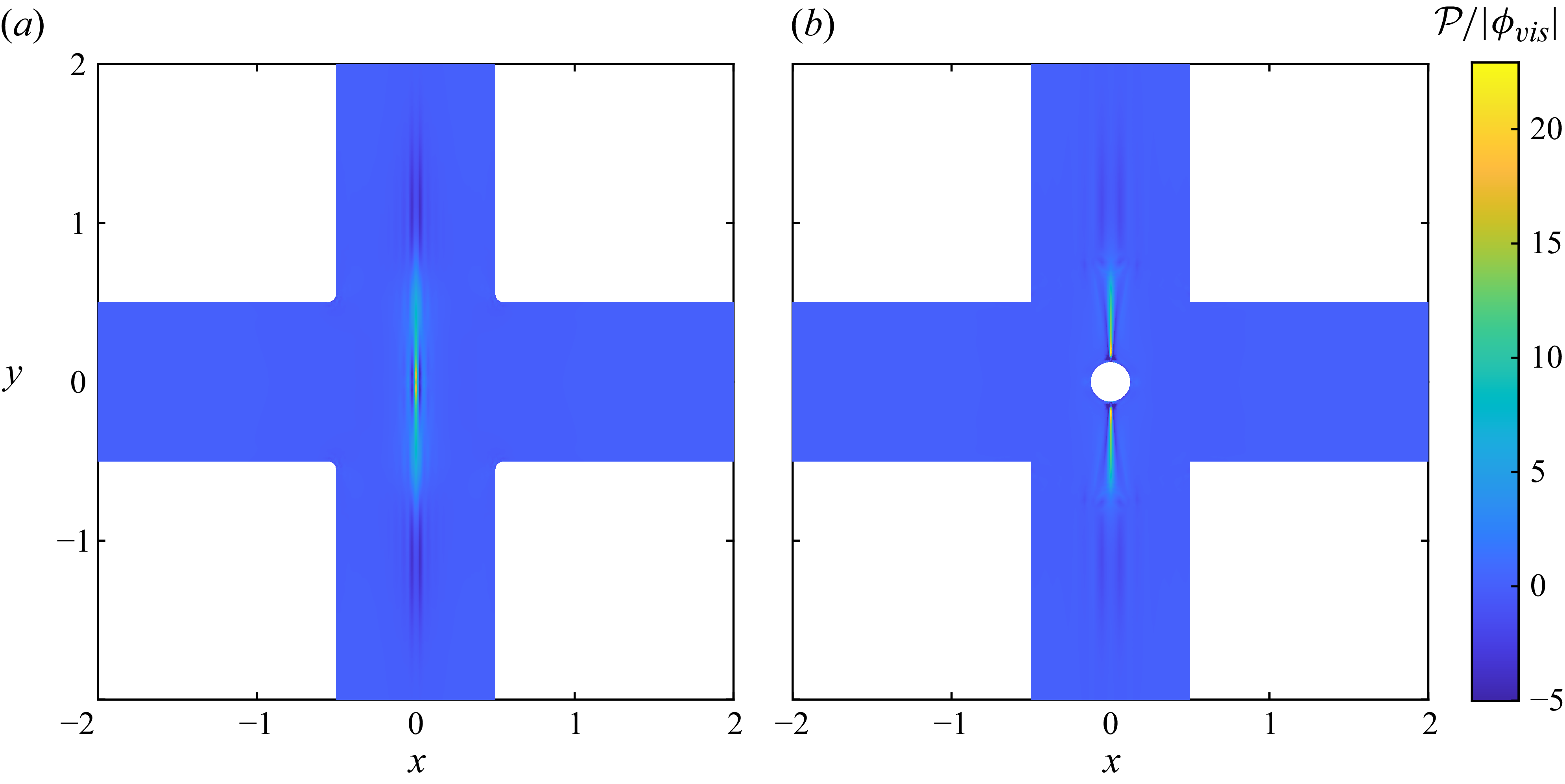
 P/|ϕvis|
 0.05
 0.25
 Wi=0.4
 ϵ=5×10⁻⁵

 ϵ=5×10⁻⁵
 ϵ=0
 Wicr=0.3676
 0.3638
 0.3616
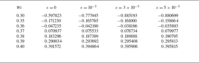
 σr
 ϵ
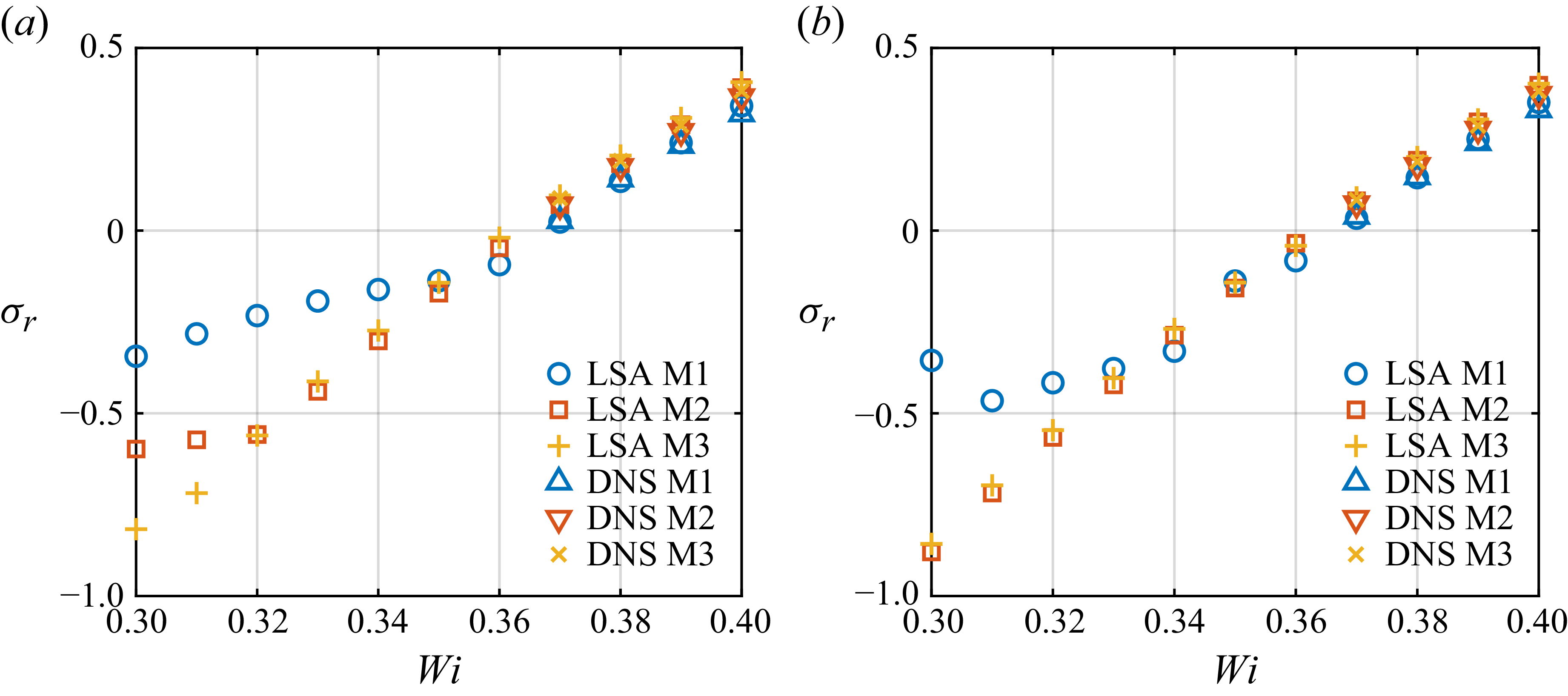
 σr
 Wi
 (a)
 ϵ=0
 (b)
 ϵ=5×10⁻⁵
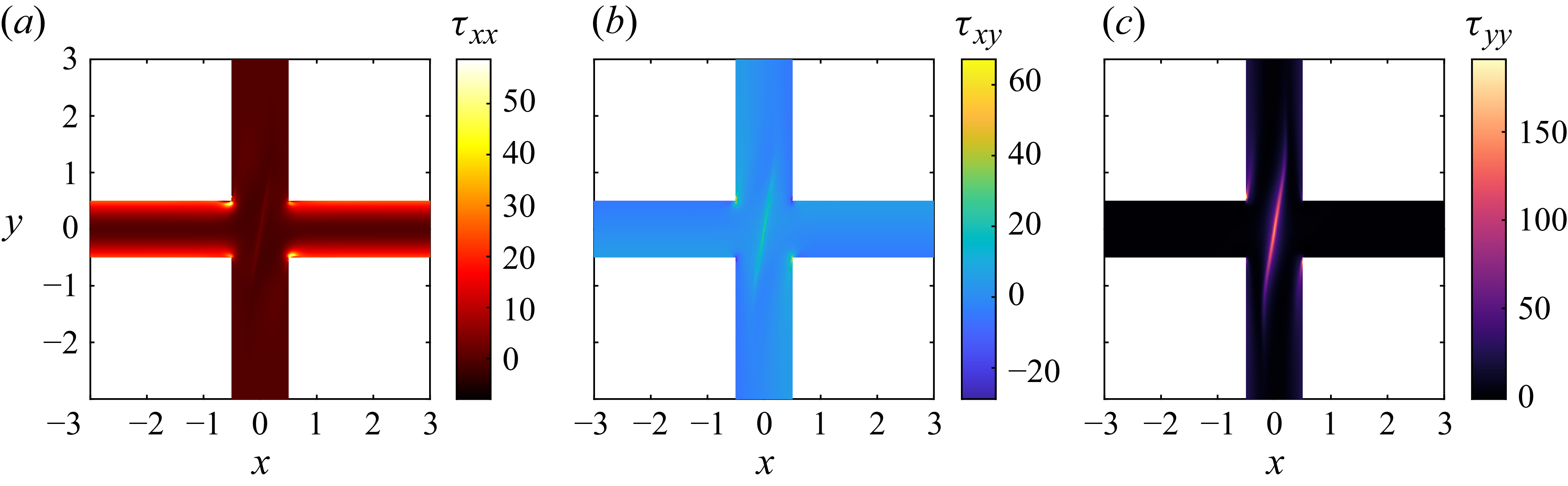
 τxx
 τxy
 τyy
 Wi=0.4
 ϵ=5×10⁻⁵

 τxxDMD(1)
 τxyDMD(1)
 τyyDMD(1)
 τxxDMD(2)
 τxyDMD(2)
 τyyDMD(2)
 Wi=0.4
 ϵ=5×10⁻⁵

 τ^xx
 τ^xy
 τ^yy
 0.05
 Wi=0.4
 ϵ=0
 0.25

 τ^xx
 τ^xy
 τ^yy
 0.05
 Wi=0.4
 ϵ=5×10⁻⁵
 0.25

 ψ^:∇u^/|ϕvis|
 Wi=0.4
 0.05
 0.25

 Open access

