a=0



1. Introduction
First-passage percolation is a probabilistic model introduced in 1965 by Hammersley and Welsh [Reference Hammersley and Welsh12] to study the flow of fluids through porous media. We refer to [Reference Auffinger, Damron and Hanson2] for a survey on the subject. We consider the lattice
 $\mathbb{Z}^d$
with all neighbouring edges of the form (x,y) such that
 $\lVert x-y\rVert_1=1$
. With each edge e, we associate a non-negative random variable
 $\tau_{e}$
with common cumulative distribution function F, called the passage time of edge e. A path is a finite or infinite sequence of edges such that consecutive edges share a unique endpoint. For such a path
 $\Gamma$
, we define
 $T(\Gamma)=\sum_{e\in\Gamma}\tau_{e}$
, which we call the passage time of
 $\Gamma$
. To define the passage time between
 $x,y\in\mathbb{R}^{d}$
, we first denote by x
′ the unique vertex in
 $\mathbb{Z}^{d}$
such that
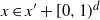 $x\in x'+[0, 1)^{d}$
. Now, if
 $x,y\in\mathbb{R}^{d}$
, we define the passage time between x and y as
 $T(x,y)=\inf_{\Gamma} T(\Gamma)$
, where this infimum is taken over the set of paths
 $\Gamma$
with endpoints x
′ and y
′. We focus on the random balls for this pseudo-distance as the fundamental objects of our study. For
 $t\geq 0$
let
 \begin{equation*} B_{t}=\{ x\in\mathbb{R}^{d}\colon T(0,x)\leq t\}\end{equation*}
be the set of points reachable from the origin in a time less than t. Most of the time, the
 $(\tau_e)_e$
are taken to be independent and identically distributed (i.i.d.). We recall in Section 1.1 the results in the i.i.d. setting that are the most relevant in the context of this article. The purpose of this article is to introduce a model of first-passage peroclation called Brochette first-passage percolation. The motivation of this novel first-passage percolation model is twofold:
-
• It can be viewed as a discrete analogue of the continuous model introduced by Aldous in [Reference Aldous1] and studied further by Kendall in [Reference Kendall13]. This model was introduced as a toy model for road networks. The analogy between the Aldous–Kendall model and Brochette first-passage percolation will be discussed in Remark 1.3.
-
• It seems to us to be a natural way of introducing infinite-range dependency in first-passage percolation.
Also, we will see that, unlike the classical case, we are able to determine the constants and limiting shapes (see Theorems 1.3 and 1.5). Moreover, a striking difference between these two models lies in the variety of possible behaviours when the time constant is zero (see Theorem 1.4).
1.1. First-passage percolation in the independent setting
A first result of the classical model is that T(0, nx) grows linearly. More precisely, we have the following result.
Theorem 1.1. ([Reference Kingman15]; see [Reference Auffinger, Damron and Hanson2, Theorem 2.1]). Assume that
 $(\tau_{e})_{e\in\mathbb{E}^{d}}$
are i.i.d. random variables such that
 $\mathbb{E}[\!\min(\tau_{1},\ldots,\tau_{2d})]<+\infty$
. Then, for all
 $x\in\mathbb{Z}^d$
, there exists a constant
 $\mu(x)\geq0$
(called the time constant) such that
 $\lim_{n\to+\infty}{T(0,nx)}/{n} =\mu(x)$
almost surely (a.s.) and in
 $L^{1}$
.
However, in this model, no non-trivial distribution is known for which the time constant
 $\mu$
can be computed. In 1981, Cox and Durrett improved this result with their shape theorem.
Theorem 1.2 ([Reference Cox and Durrett7]). Assume now that
 $\mathbb{E}[\!\min(\tau_{1}^{d},\ldots,\tau_{2d}^{d})]<+\infty$
and that
 $F(0) < p_{\mathrm{c}}(d)$
, where
 $p_{\mathrm{c}}(d)$
is the critical parameter for bond percolation in
 $\mathbb{Z}^{d}$
. Then, there exists a deterministic, compact, and convex subset
 $B_{\ast}$
of
 $\mathbb{R}^{d}$
such that, for all
 $\varepsilon>0$
,
 \begin{equation*} \mathbb{P}\big((1-\varepsilon)B_{\ast}\subset{B_{t}}/{t}\subset(1+\varepsilon)B_{\ast}\ { for\ all\ large }\ t\big) = 1. \end{equation*}
Furthermore,
 $B_{\ast}$
is symmetric with respect to the axes of
 $\mathbb{R}^{d}$
and has a non-empty interior.
Several slightly different models have been introduced, we mention two cases in particular:
-
• The case where no integrability condition holds for
 $\tau$
, in particular where
$\mathbb{P}(\tau=+\infty)>0$
, has also been studied, notably in [Reference Garet and Marchand11] and [Reference Cerf and Théret5]. They also proved an analogue of Theorem 1.1 with convergence in probability.
-
• The case where passage times are non-independent. For example, the stationary ergodic case was studied in [Reference Boivin4]. This model, still rich, has led to many results analogous to the classical ones.


In contrast, in this article we consider a long-range dependence model, which, to our knowledge, has not yet been studied. The name of this model is inspired by the one studied in [Reference Duminil-Copin, Hilario, Kozma and Sidoravicius9] in the context of bond percolation. As in that article, we introduce a strong dependence along the lines.
1.2. Brochette first-passage percolation
As in the classical case we consider the graph
 $(\mathbb{Z}^{d},\mathbb{E}^{d})$
. In this model, the passage times associated with edges on the same line are equal. However, the passage times associated with edges on distinct lines are still independent. Let us now define our model more formally.
Definition 1.1. An integer line is the set of points in
 $\mathbb{Z}^{d}$
that lie on the same line in
 $\mathbb{R}^{d}$
parallel to one of the axes. We denote by
 $\Delta$
the set of these lines.
Definition 1.2 (Brochette first-passage percolation). Let
 $(\tau_{\delta})_{\delta\in\Delta}$
be a family of non-negative i.i.d. random variables with common cumulative distribution function F and indexed by the set of integer lines. In Brochette first-passage percolation we associate the same passage time to all edges whose endpoints lie on the same integer line
 $\delta\in\Delta$
. In other words, for an edge
 $e\in\mathbb{E}^d$
, the passage time
 $\tau_e$
of e is equal to
 $\tau_\delta$
, where
 $\delta$
is the unique integer line to which e belongs.
From now on, T and
 $B_t$
denote passage times and random balls for Brochette first-passage percolation. Throughout the paper we assume that the support of our passage times is included in an interval of the form
 $[a,+\infty)$
, where
 $a\geq 0$
and a equals the infimum of this support. In particular, we will use that
 \begin{equation} \text{for all } \delta>0,\ F(a+\delta)>0 \quad \text{ and }\quad F(a-\delta)=0.\end{equation}
In the Brochette model, T(0, n) is more sensitive to small values of passage times. Small passage times generate kinds of highways that geodesics tend to go through. Thus, the random balls do not look alike for the classical and the Brochette models. (See the simulations in Figures 1 and 2.)
The random balls
 $B_t$
for
 $t=500$
for the distribution
 $1+\mathrm{Bernoulli}(0.95)$
for the classical model (on the left) and the Brochette model (on the right).

The random balls
 $B_t$
for
 $t=5$
for the uniform distribution on [0, 1] for the classical model (on the left) and the Brochette model (on the right) (cf. [Reference Blanc3, Figure 1]). Observe that we need to plot balls with much smaller radii than in Figure 1.

1.3. Results
Our first result is that we can identify the time constant in the Brochette model.
Theorem 1.3 (Point-to-point convergence theorem). For Brochette first-passage percolation, if we assume that
 \begin{equation} \mathbb{E}\lbrack \!\min(\tau_{1},\ldots,\tau_{d})\rbrack<+\infty, \end{equation}
where
 $\tau_{1},\ldots,\tau_{d}$
are d independent copies with distribution F, then, for all
 $x\in\mathbb{Z}^{d}$
,
 \begin{equation*}\lim_{n\rightarrow+\infty}\frac{T(0,nx)}{n}=a\lVert x\rVert_1\end{equation*}
a.s. and in
 $L^{1}$
, where we recall that a is the infimum of the support of
 $\tau$
.
Observe that, by the definition of a,
 $T(0,x)\geq a\lVert x\rVert_1$
almost surely, so the non-trivial part of Theorem 1.3 is the upper bound.
Remark 1.1. Note that Assumption (1.2) is not the same as in the i.i.d. case, as there are d independent integer lines passing through each vertex instead of 2d edges as in the classical model. It follows that (1.2) is optimal. Indeed, if Assumption (1.2) is not satisfied
 $T(0,e_{1})$
is not integrable.
Theorem 1.3 states that in the case
 $a=0$
, T(0, n) is sublinear, with the exact order of magnitude yet to be determined. In the classical model, it is known that
 $\mathbb{E}[T(0,n)]$
is sublinear as soon as
 $F(0)\geq p_{\mathrm{c}}$
(see [Reference Kesten14, Theorem 1.15]). Several works tried to better understand the behaviour of
 $\mathbb{E}[T(0,n)]$
in this case. First, [Reference Zhang17] established that
 $\mathbb{E}[T(0,n)]$
remains bounded if
 $F(0)>p_{\mathrm{c}}$
. The case
 $F(0)=p_{\mathrm{c}}$
is more subtle. We mention a few results in dimension
 $d=2$
: [Reference Chayes, Chayes and Durrett6] proved that if F is a Bernoulli distribution of parameter
 $p_{\mathrm{c}}$
, then there exist
 $C_1,C_2>0$
such that
 $C_1\log(n)\leq\mathbb{E}[T(0,n)]\leq C_2\log(n)$
for all n large enough; also, [Reference Zhang18] showed that there are some distributions F such that
 $F(0)=p_{\mathrm{c}}$
for which
 $\mathbb{E}[T(0,n)]$
converges to a non-negative constant (see also [Reference Damron, Lam and Wang8] for more related results). We will see that, for the Brochette model, depending on the behaviour of the distribution function F of the passage times near 0, a wide variety of behaviours can emerge even in dimension
 $d=2$
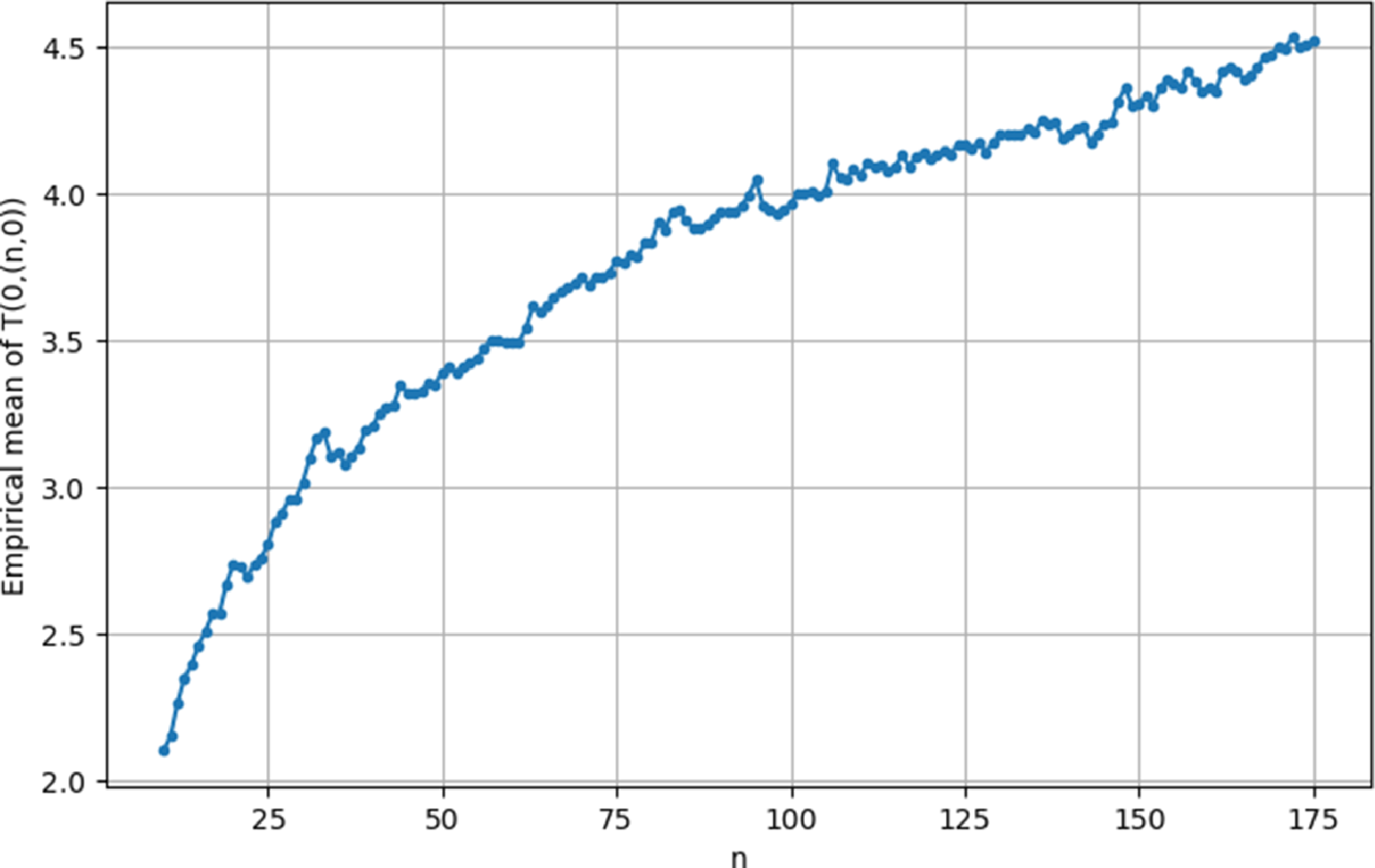
. (See Figure 3 for a graphical representation of the empirical mean of
 $T(0,(n,0))$
as a function of
 $n$
for the uniform distribution on
 $[0,1]$
.)
Theorem 1.4. Consider Brochette first-passage percolation with
 $a=0$
in dimension
 $d=2$
. If there exist
 $C>0,\beta\geq0$
such that
 $F(t)\sim_{t\rightarrow 0+}Ct^{\beta}$
, and if the passage times are bounded and atomless, then for all
 $x\in\mathbb{Z}^{2}$
there exist
 $A_1,A_2>0$
such that, for all
 $n\geq2$
,
-
(i) If
$\beta<1$
,
$A_1\leq \mathbb{E}[T(0,nx)]\leq A_2$
. -
(ii) If
$\beta=1$
,
$A_1 \log(n)\leq \mathbb{E}[T(0,nx)]\leq A_2 \log(n)$
. -
(iii) If
$\beta>1$
,
$A_1n^{1-{1}/{\beta}}\leq \mathbb{E}[T(0,nx)]\leq A_2n^{1-{1}/{\beta}}$
.






Remark 1.2. We could not obtain comparable results in higher dimensions, which is why we focus on the case
 $d=2$
.
Empirical mean of T(0, (n, 0)) for 200 independent configurations where the passage times follow a uniform distribution on [0, 1].

Remark 1.3. As stated earlier, we can see an analogy between Brochette first-passage percolation for
 $a=0$
and the Aldous–Kendall model. Specifically, that model is defined through a Poisson random measure
 $\Pi$
on
 $\mathbb{L}^d\times \mathbb{R}^{\ast}_{+}$
whose intensity is proportional to
 $\mu_d\otimes v^{-\gamma}\mathrm{d}v$
, where
 $\gamma>d$
is a parameter,
 $\mathbb{L}^d$
is the set of affine lines of
 $\mathbb{R}^d$
, and
 $\mu_d$
is its invariant measure. Each atom
 $(\ell,v)\in\mathbb{L}^d\times \mathbb{R}^{\ast}_{+}$
of
 $\Pi$
is seen as a road of speed limit v. They then consider the passage time
 $\mathcal{T}(x,y)$
for all
 $x,y\in\mathbb{R}^d$
using these roads.
To compare both models, let us make the following observation. A unit segment of a road has a speed limit larger than
 $\varepsilon^{-1}$
with a probability of order
 $(1/\varepsilon)^{-\gamma+1}$
. Thus, the time to cross this segment is smaller than
 $\varepsilon$
with the same probability. It corresponds to taking
 $\beta=\gamma-1$
in Theorem 1.4. In the Aldous–Kendall model, by the properties of the Poisson point process we have the scaling
 \begin{equation*} \mathcal{T}(0,nx) \overset{(\mathrm{d})}{=} (n\lVert x \rVert)^{({\gamma-2})/({\gamma-1})}\mathcal{T}(0,e_1) = (n\lVert x \rVert)^{1-{1}/{\beta}}\mathcal{T}(0,e_1) \end{equation*}
for any
 $\gamma>2$
. Theorem 1.4(iii) shows that we have the same asymptotics for
 $\beta>1$
in our model. Of course, the scaling argument doesn’t apply here due to the discrete structure of
 $\mathbb{Z}^2$
.
The third result is the shape theorem. We denote by
 $\Diamond$
the closed unit ball for the
 $L^1$
norm.
Theorem 1.5. For Brochette first-passage percolation, if we assume that
 \begin{equation} \mathbb{E} \big[\!\min \big(\tau_{1}^{d},\ldots,\tau_{d}^{d} \big)\big]<+\infty \end{equation}
and that
 $a>0$
satisfies (1.1), then for all
 $\varepsilon>0$
we have
 \begin{equation*} \mathbb{P}\bigg(\frac{1-\varepsilon}{a}\Diamond \subset \frac{B_{t}}{t} \subset \frac{1}{a}\Diamond \text{ for all large }t\bigg)=1. \end{equation*}
Furthermore, if
 $a=0$
we have, for all
 $M>0$
,
 $\mathbb{P}(M\Diamond \subset {B_{t}}/{t} \text{ for all large } t)=1$
.
Remark 1.4. We will see in Proposition 4.1 that Theorem 1.5 holds only if Condition (1.3) is satisfied. Otherwise, there is no shape theorem in the sense of double inclusion.
Finally, we consider one last case: when
 $\mathbb{P}(\tau=+\infty)>0$
. This case amounts to studying first-passage percolation on the cluster
 $\mathcal{C}_{\ast}$
composed of lines whose passage times are finite. Moreover, as soon as
 $\mathbb{P}(\tau<+\infty)>0$
the subgraph obtained is both connected and infinite, whereas this is not the case in the classical model. Indeed, if an edge has a finite passage time, then all the edges on the same line have the same finite passage time. Thus, it is easy to see that the subgraph is a union of integer lines. In order to state Theorem 1.6, we need to introduce a generalized notion of passage time.
Definition 1.3. If
 $x,y\in\mathbb{Z}^{d}$
, let
 $T^{\ast}(x,y)=T(x^{\ast},y^{\ast})$
, where
 $x^{\ast}$
is the closest vertex in the
 $L^{1}$
norm to x in the cluster of edges with finite passage times, with an arbitrary rule to break ties.
Theorem 1.6. For Brochette first-passage percolation, if
 $\mathbb{P}(\tau<+\infty)>0$
then, for all
 $x\in\mathbb{Z}^{d}$
,
 $\lim_{n\rightarrow+\infty}({T^{\ast}(0,nx)}/{n})=a\lVert x \rVert_1$
in probability.
This is the analogue of [Reference Cerf and Théret5, Theorem 4], and we follow the same proof structure. An important difference is that [Reference Cerf and Théret5] relies on non-trivial estimates in classical percolation. In our case, the infinite cluster has a rather simple shape, which allows for self-contained proofs. Although the proof of Theorem 1.6 is partly identical to that in [Reference Cerf and Théret5], we have nevertheless chosen to present it in detail for the sake of readability. Moreover, due to the dependence, the estimates on the percolation clusters are different in the Brochette model (see Lemma 5.1).
To conclude, we outline how the different sections of this article will be structured.
-
• In Section 2 we focus on point-to-point convergence and prove Theorem 1.3.
-
• In Section 3 we prove Theorem 1.4 about the variety of behaviours for the expectation of the passage time in dimension
$d=2$
. -
• In Section 4 we obtain a shape theorem by proving Theorem 1.5.
-
• In Section 5 we prove Theorem 1.6 about the convergence in probability of
${T^{\ast}(0,nx)}/{n}$
.


2. Point-to-point almost sure convergence
This section is devoted to the proof of Theorem 1.3: the almost sure convergence of
 ${T(0,nx)}/{n}$
. In addition to proving the linear growth of the passage time we are able to determine the limit constant, which is equal to
 $a \lVert x \rVert_1$
. This is a first step towards understanding the behaviour of T(0, x) in the context of Brochette first-passage percolation. This result will be improved in Section 4.
Proof of Theorem 1.3. To prove this theorem we will use the following version of Kingman’s theorem.
Theorem 2.1 (Subadditive ergodic theorem [Reference Liggett16]). Let
 $(X_{m,n})_{0\leq m\leq n}$
be a family of random variables that satisfy the following assumptions:
-
(i)
$X_{0,n}\leq X_{0,m}+X_{m,n}$
for all
$0<m<n$
. -
(ii) The sequences
$(X_{m,m+k})_{k\geq1}$
and
$(X_{m+1,m+k+1})_{k\geq1}$
have the same distribution for all
$m\geq0$
. -
(iii) For all
$k\geq1$
, the sequence
$(X_{nk,(n+1)k})_{n\geq0}$
is stationary. -
(iv)
$\mathbb{E}\lbrack X_{0,1} \rbrack<+\infty$
and
$\mathbb{E}\lbrack X_{0,n} \rbrack>-cn$
for some finite constant c.






Then there exists a random variable X such that
 ${X_{0,n}}/{n}\rightarrow_{n\rightarrow+\infty}X$
a.s. and in
 $L^{1}$
.
Fix
 $x\in\mathbb{Z}^{d}$
. We aim to apply Theorem 2.1 to
 $X_{m,n}=T(mx,nx)$
. We verify briefly that (i)–(iv) hold. (i) is immediate. As in the i.i.d. case, the environment is invariant under shifts of
 $\mathbb{Z}^{d}$
so assumptions (ii) and (iii) hold. Moreover,
 $\mathbb{E}[X_{0,n}]>-cn$
because passage times are non-negative. It remains to prove that
 $E[X_{0,1}]<+\infty$
. There exist d paths
 $\Gamma_1,\ldots,\Gamma_d$
from 0 to x whose passage times are independent. Thus,
 $T(0,x)\leq \min(T(\Gamma_1),\ldots,T(\Gamma_d))$
and if we let L be the length of the longest of these paths (say
 $\Gamma_1$
) we have
 \begin{align*} \mathbb{P}(T(0,x)>s) & \leq \mathbb{P}\Bigg(\bigcap_{i=1}^{d}\{T(\Gamma_i)>s\}\Bigg) \\ & = \prod_{i=1}^{d}\mathbb{P}(T(\Gamma_i)>s) \\ & \leq \mathbb{P}(T(\Gamma_1)>s)^d = \bigg(L\mathbb{P}\bigg(\tau_e>\frac{s}{L}\bigg)\bigg)^d. \end{align*}
Therefore, considering
 $Y\,:\!=\,\min(\tau_1,\ldots,\tau_d)$
, where
 $\tau_1,\ldots,\tau_d$
are i.i.d. with the same distribution F, we have
 $\mathbb{P}(T(0,x)>s)\leq L^d\mathbb{P}(Y>{s}/{L})$
, from which we deduce, thanks to (1.2), that
 $\mathbb{E}[X_{0,1}]<+\infty$
. Kingman’s theorem therefore implies that there exists a random variable
 $X_x$
such that
 $\lim_{n\rightarrow+\infty}{T(0,nx)}/{n}=X_x$
a.s. and in
 $L^{1}$
.
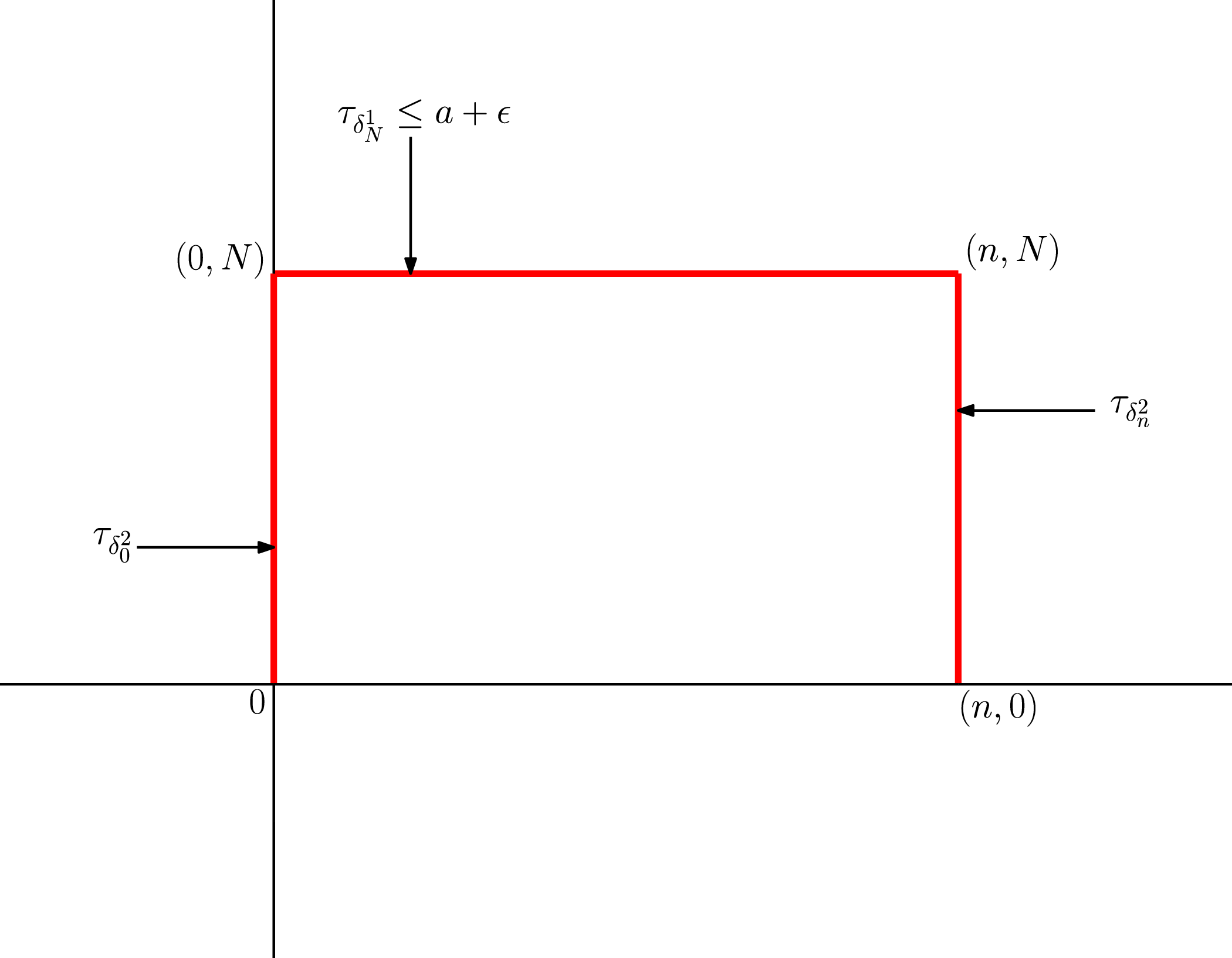
The path going from 0 to
 $ne_1$
following the construction.

We first prove that for
 $x=e_1$
it suffices to show that, for all
 $\varepsilon >0$
,
 $\liminf {T(0,ne_1)}/{n}\leq a+\varepsilon$
a.s. Let
 $\varepsilon>0$
. We denote by
 $\delta_k^1$
the line
 $ke_2+\mathbb{Z} e_1$
with
 $e_2\,:\!=\,(0,1,0,\ldots,0)$
. Let
 $N=\inf\{ k\geq 1, \tau_{\delta_k^1}\leq a+\varepsilon\}$
. Since
 $(\delta_k^1)_{k\in \mathbb{N}}$
are i.i.d. and by the definition of a,
 $N<+\infty$
a.s. Let
 $\delta_k^2$
be the line
 $ke_1+\mathbb{Z} e_2$
(see Figure 4). Then
 $T(0,ne_1)\leq N \tau_{\delta_0^2}+ n(a+\varepsilon)+ N\tau_{\delta_n^2}$
, and thus
 \begin{equation*} \frac{T(0,ne_1)}{n}\leq \frac{N}{n}\tau_{\delta_0^2}+(a+\varepsilon)+ \frac{N}{n}\tau_{\delta_n^2}. \end{equation*}
Since
 $N<+\infty$
almost surely, doesn’t depend on n, and
 $\tau_{\delta_0^2}<+\infty$
almost surely too, we have
 $\lim_{n\to+\infty}({N}/{n})\tau_{\delta_0^2}=0$
. Moreover, since
 $(\tau_{\delta_n^2})_n$
are i.i.d. with distribution F, they are infinitely often smaller than
 $a+1$
and we have
 $\liminf_{n\to+\infty}({N}/{n})\tau_{\delta_n^2}=0$
. We conclude that
 \begin{equation*} \liminf_{n\to+\infty} \frac{T(0,ne_1)}{n}\leq a+\varepsilon\ \text{a.s.} \end{equation*}
Therefore,
 $\lim_{n\to+\infty}{T(0,ne_1)}/{n}=a$
a.s. and in
 $L^1$
. Now, let
 $x=(x_1,\ldots,x_d)\in\mathbb{N}^d$
(the proof for
 $x\in\mathbb{Z}^d$
is the same). Let
 $y_i=(x_1,\ldots,x_i,0,\ldots,0)$
. Then
 \begin{equation*} T(0,nx)\leq \sum_{i=0}^{d-1} T(ny_i,ny_{i+1}). \end{equation*}
Since
 $T(ny_i,ny_{i+1})\overset{(\mathrm{d})}{=}T(0,nx_{i+1}e_{i+1})$
, we have
 ${T(ny_i,ny_{i+1})}/{n}\rightarrow_{n\rightarrow+\infty}ax_{i+1}$
in probability. Thus, we get

3. The case
$\boldsymbol{a}=0$

In this section, we study the case where
 $a=0$
and
 $d=2$
. We will see that, depending on F, a diverse range of behaviours for T(0, n) can arise. For this purpose we define the following random variable.
Definition 3.1. If
 $\tau_{1},\ldots,\tau_{n}$
are independent passage times, we write
 $M_{n}\,:\!=\,\min(\tau_{1},\ldots,\tau_{n})$
.
To prove Theorem 1.4, we will see it as a corollary of the following theorem.
Theorem 3.1. For Brochette first-passage percolation when
 $d=2$
, if
 $a=0$
with a defined by (1.1), if the distribution of
 $\tau$
is atomless, and if we assume that
 $\mathbb{E}[min(\tau_{1},\tau_{2})]<+\infty$
, then, for all
 $x\in \mathbb{Z}^{2}$
,
 \begin{equation*} \sum_{k=0}^{\lVert nx \rVert_1-1}\mathbb{E}[M_{4k+2}] \leq \mathbb{E}[T(0,nx)] \leq 8\sum_{k=0}^{\lVert nx\rVert_1-1}\mathbb{E}[M_{k}]. \end{equation*}
Proof. Let us denote by
 $X_{n}$
the random variable equal to the abscissa of the vertical edges with the smallest passage time in
 $[\![ 0,n]\!]^{2}$
, and by
 $Y_{n}$
the random variable equal to the ordinate of the horizontal edges with the smallest passage time in
 $[\![ 0,n ]\!]^{2}$
. We write
 $I_{n}\,:\!=\,T(0,(X_{n},Y_{n}))$
, with
 $I_0\,:\!=\,0$
. Then, by subadditivity, we have
 $I_{n+1}-I_{n}\leq T((X_{n},Y_{n}),(X_{n+1},Y_{n+1}))$
, which gives
 $\mathbb{E}[I_{n+1}-I_{n}]\leq \mathbb{E}[T((X_{n},Y_{n}),(X_{n+1},Y_{n+1}))]$
.
Now, if
 $(X_{n+1},Y_{n+1})\neq (X_{n},Y_{n})$
, we have
 \begin{equation*} (X_{n+1},Y_{n+1})\in\{(X_{n},n+1),(n+1,Y_{n}),(n+1,n+1)\}. \end{equation*}
Moreover,
 $X_{n}$
and
 $Y_{n}$
are independent and, since the passage times are atomless, we have
 \begin{equation*} \mathbb{P}(X_{n+1}=n+1)=\mathbb{P}(Y_{n+1}=n+1)=\frac{1}{n+2}. \end{equation*}
Let
 $T_{n,n+1}\,:\!=\,T((X_{n},Y_{n}),(X_{n+1},Y_{n+1}))$
. If
 $n\in \mathbb{N}$
, we denote by
 $\tau_{v,n}$
the passage time associated with the vertical integer line of abscissa n, and by
 $\tau_{h,n}$
the passage time associated with the horizontal integer line of ordinate n. We have:
-
• If
$(X_{n+1},Y_{n+1})=(X_{n},n+1)$
,
$T_{n,n+1}\leq (n+1)\tau_{v,X_{n}}$
. -
• If
$(X_{n+1},Y_{n+1})=(n+1,Y_{n})$
,
$T_{n,n+1}\leq (n+1)\tau_{h,Y_{n}}$
. -
• If
$(X_{n+1},Y_{n+1})=(n+1,n+1)$
,
$T_{n,n+1}\leq (n+1)\tau_{v,X_{n}}+(n+1)\tau_{h,n+1}$
.






Finally, since
 $X_n$
is independent of the horizontal passage times and
 $Y_n$
is independent of the vertical passage times, we have
 \begin{align*} \mathbb{E}[I_{n+1}-I_{n}] & \leq \mathbb{E}[T_{n,n+1}] \\ & = \mathbb{E}[T_{n,n+1}\mathbf{1}_{(X_{n+1},Y_{n+1})=(X_{n},n+1)}] + \mathbb{E}[T_{n,n+1}\mathbf{1}_{(X_{n+1},Y_{n+1})=(n+1,Y_{n})}] \\ & \quad + \mathbb{E}[T_{n,n+1}\mathbf{1}_{(X_{n+1},Y_{n+1})=(n+1,n+1)}] \\ & \leq \mathbb{E}[(n+1)\tau_{v,X_{n}}\mathbf{1}_{(X_{n+1},Y_{n+1})=(X_{n},n+1)}] + \mathbb{E}[(n+1)\tau_{h,Y_{n}}\mathbf{1}_{(X_{n+1},Y_{n+1})=(n+1,Y_{n})}] \\ & \quad + \mathbb{E}[((n+1)\tau_{v,X_{n}}+(n+1)\tau_{h,n+1})\mathbf{1}_{(X_{n+1},Y_{n+1})=(n+1,n+1)}] \\ & \leq \mathbb{E}[\tau_{v,X_{n}}\mathbf{1}_{X_{n+1}=X_{n}}] + \mathbb{E}[\tau_{h,Y_{n}}\mathbf{1}_{Y_{n+1}=Y_{n}}] + \mathbb{E}[\tau_{v,X_{n}}\mathbf{1}_{X_{n+1}=n+1}] \\ & \quad + \mathbb{E}[\tau_{h,n+1}\mathbf{1}_{Y_{n+1}=n+1}] \leq 2\mathbb{E}[M_{n}]. \end{align*}
Hence, by summing, we obtain
 $\mathbb{E}[I_{n}]\leq 2 \sum_{k=0}^{n-1} \mathbb{E}[M_{k}]$
. Moreover, to go from 0 to (n,0), we can use the same method to construct a path from (n,0) to
 $(X_{n},Y_{n})$
. We can do the same computation and obtain
 $\mathbb{E}[T(0,(n,0))]\leq 2\mathbb{E}[I_{n}]$
. Now, to go from 0 to
 $x=(x_{1},x_{2})$
, we can use the same method twice to go from 0 to
 $(x_{1},0)$
and then from
 $(x_{1},0)$
to
 $(x_{1},x_{2})$
. It follows that, by telescoping, we have
 \begin{equation*} \mathbb{E}[T(0,nx)] \leq 4\mathbb{E}[I_{\lVert nx\rVert_1 }]\leq8\sum_{k=0}^{\lVert nx\rVert_1-1}\mathbb{E}[M_{k}]. \end{equation*}
For the lower bound we proceed differently. We note that to go from 0 to nx, a path must cross all the deterministic
 $L^1$
balls of radius k for k between 0 and
 $\lVert nx\rVert_1-1$
. Thus, the passage time from 0 to nx is greater than the sum of the minimum passage times among the edges of the sphere of radius k for k ranging from 0 to
 $\lVert nx\rVert_1-1$
. Moreover, in dimension 2,
 $4k+2$
independent edges originate from a vertex on the sphere of radius k. Thus,
 \begin{equation*} \sum_{k=0}^{\lVert nx \rVert_1-1}\mathbb{E}[M_{4k+2}]\leq \mathbb{E}[T(0,nx)]. \end{equation*}
4. Shape theorem
This section is devoted to the proof of Theorem 1.5. First, by the definition of our model,
 ${B_{t}}/{t}\subset ({1}/{a})\Diamond$
for all t. Only the first inclusion remains to be proven. To improve a pointwise convergence into a shape theorem, all the usual proofs rely at some point on uniform control of T(x,y). To obtain such control, we prove here the analogue of the difference estimate lemma [Reference Auffinger, Damron and Hanson2, Lemma 2.20]. This step follows the same strategy as developed in [Reference Cox and Durrett7] but presents a particular difficulty in the Brochette case. As we will see, the dependence makes the construction of certain paths more delicate.
Lemma 4.1. Consider Brochette first-passage percolation and assume that we have the integrability condition (1.3). Then, there exists a constant
 $\kappa>0$
such that, for every
 $z\in\mathbb{Z}^{d}$
,
 \begin{equation*} \mathbb{P}\bigg({\sup\nolimits_{{x\in\mathbb{Z}^{d},\,x\neq z}}}\frac{T(z,x)}{\lVert x-z \rVert_1}<\kappa\bigg)>0. \end{equation*}
Proof. By shift invariance, it is sufficient to prove the result for
 $z=0$
. We provide all the details of the proof in the case
 $d=2$
and then briefly explain at the end how to generalize it to an arbitrary d.
Set
 $x=(x_1,x_2)$
. Without loss of generality, we assume that
 $x_1\geq x_2\geq 0$
. Similarly to the classical proofs, the estimates will rely on the construction of paths from 0 to x.
-
• We first construct
$(d+1)=3$
paths
$\Gamma_1, \Gamma_2, \Gamma_3$
that primarily use edges whose passage times are independent of most of the edges in the other paths. -
• Then, for
$1\leq i\leq 3$
, we will bound
$\mathrm{Var}(T(\Gamma_i))$
. To do this, we decompose each
$\Gamma_i$
into several segments, which we call steps, and most of these are independent. -
• In the last step of the proof, we exploit the fact that
$\Gamma_1$
,
$\Gamma_2$
, and
$\Gamma_3$
are mostly independent in order to control T(0, x).


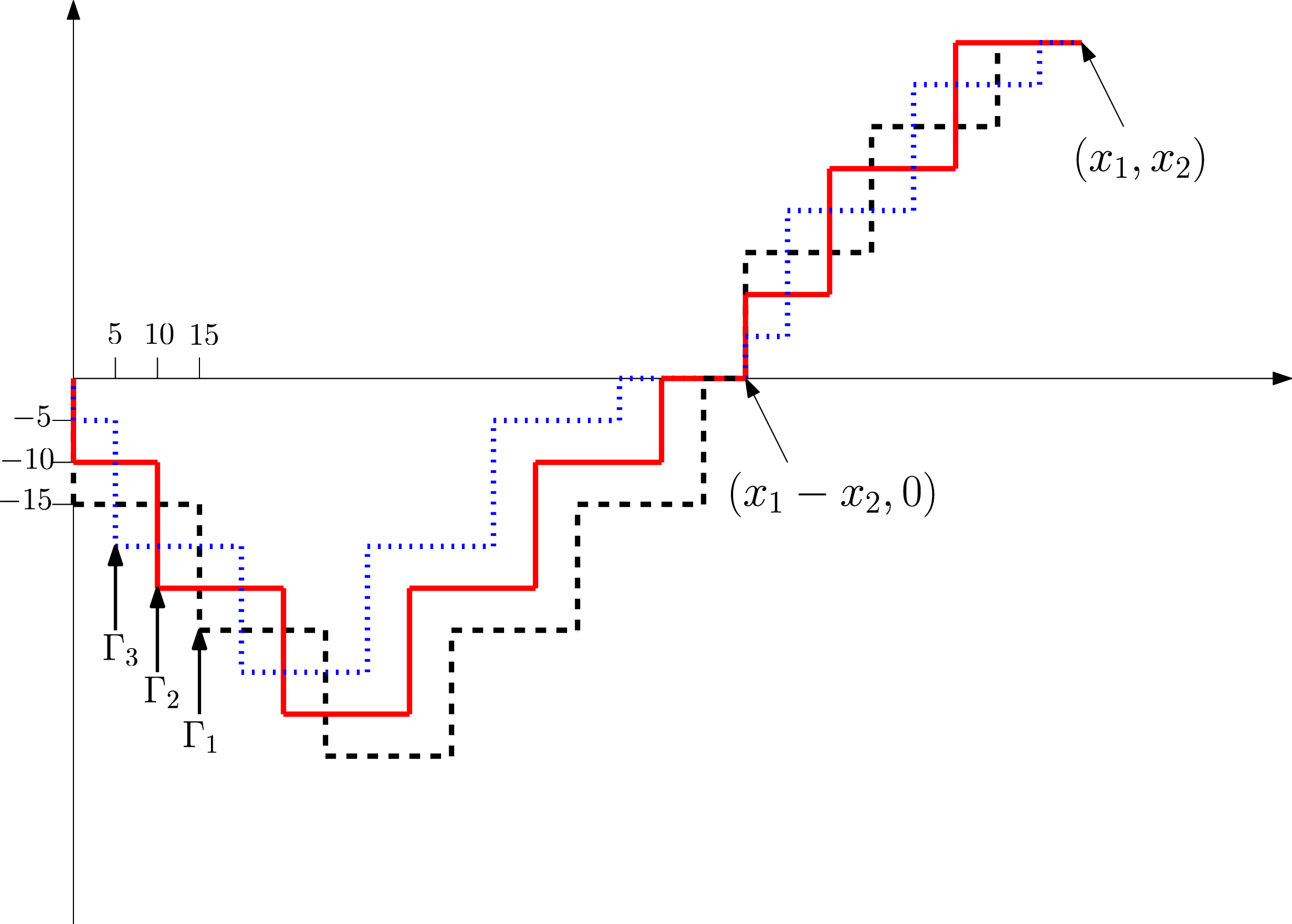
Paths
 $\Gamma_1,\Gamma_2,\Gamma_3$
.

Construction of paths
 $\Gamma_{1},\Gamma_2,\Gamma_3$
. (See Figure 5). We begin by defining a deterministic path
 $S_{1}$
from 0 to x, which we will refer to as the skeleton. It is composed of three staircases: it descends and then ascends to
 $(x_1-x_2,0)$
before ending at
 $(x_1,x_2)$
. Formally, if
 \begin{equation*}p=\bigg\lfloor \frac{x_1-x_2}{15}\bigg\rfloor, \qquad p'=\bigg\lfloor\frac{x_2}{15}\bigg\rfloor,\end{equation*}
then
 $S_1$
is the path that passes through the points
 \begin{align*} x^{1}_0 = (0,0) & \rightarrow x^{1}_1 = (0,-15) \\ & \rightarrow x^{1}_2 = (15,-15) \\ & \rightarrow\dots\rightarrow x^{1}_{2\lceil{p}/{2}\rceil} = (\lceil{p}/{2}\rceil 15,-\lceil{p}/{2}\rceil 15) \\ & \rightarrow x^{1}_{2\lceil{p}/{2}\rceil+1} = (\lceil{p}/{2}\rceil 15,-(\lceil{p}/{2}\rceil-1)15) \\ & \rightarrow x^{1}_{2\lceil{p}/{2}\rceil+2} = ((\lceil{p}/{2}\rceil+1) 15,-(\lceil{p}/{2}\rceil-1)15) \\ & \rightarrow\dots\rightarrow x^{1}_{m_1} = (x_1-x_2,0) \\ & \rightarrow x^{1}_{m_1+1} = (x_1-x_2,15) \\ & \rightarrow x^{1}_{m_1+2} = (x_1-x_2+15,15) \rightarrow\dots\rightarrow x^{1}_{m_1+n_1} = (x_1,x_2), \end{align*}
such that between two consecutive points
 $x^{1}_i$
it follows the straight line. Note that
 $x^{1}_i$
and
 $x^{1}_{i+1}$
are almost always at most 15 edges apart. Depending on the value of p and p
′,
 $m_1\in \{4\lceil {p}/{2}\rceil-1,4\lceil {p}/{2}\rceil\}$
and
 $n_1\in\{2p',2p'+2\}$
. Similarly, we construct two other skeletons with the same shape but slightly offset from
 $S_1$
for independence reasons that will become clear later in the proof.
 $S_2$
goes through
 \begin{align*} x^{2}_0=(0,0) & \rightarrow x^{2}_1 = (0,-10) \\ & \rightarrow x^{2}_2 = (10,-10) \\ & \rightarrow x^{2}_3 = (10,-25) \\ & \rightarrow\dots\rightarrow x^{2}_{2\lceil{p}/{2}\rceil} = (10+(\lceil{p}/{2}\rceil-1)15,-10-(\lceil{p}/{2}\rceil-1) 15) \\ & \rightarrow x^{2}_{2\lceil{p}/{2}\rceil+1} = (10+(\lceil{p}/{2}\rceil-1)15,-10-(\lceil{p}/{2}\rceil-2)15) \\ & \rightarrow\dots\rightarrow x^{2}_{4\lceil{p}/{2}\rceil-1} = ((2\lceil{p}/{2}\rceil-1)15-5,0) \\ & \rightarrow x^{2}_{4\lceil{p}/{2}\rceil=:m_2}=(x_1-x_2,0) \\ & \rightarrow x^{2}_{m_2+1} = (x_1-x_2,10) \\ & \rightarrow x^{2}_{m_2+2} = (x_1-x_2+10,10) \\ & \rightarrow x^{2}_{m_2+3} = (x_1-x_2+10,10+15) \\ & \rightarrow x^{2}_{m_2+4} = (x_1-x_2+10+15,10+15) \rightarrow\dots\rightarrow x^{2}_{m_2+n_2}=(x_1,x_2), \end{align*}
with
 $n_2\in\{2p'+2;\,2p'+4\}$
.
 $S_3$
goes through
 \begin{align*} x^{3}_0 = (0,0) & \rightarrow x^{3}_1 = (0,-5) \\ & \rightarrow x^{3}_2 = (5,-5) \\ & \rightarrow x^{3}_3 = (5,-20) \\ & \rightarrow\dots\rightarrow x^{3}_{2\lceil{p}/{2}\rceil} = (5+(\lceil{p}/{2}\rceil-1)15,-5-(\lceil{p}/{2}\rceil-1)15) \\ & \rightarrow x^{3}_{2\lceil{p}/{2}\rceil+1} = (5+(\lceil{p}/{2}\rceil-1)15,-5-(\lceil{p}/{2}\rceil-2)15) \\ & \rightarrow\dots\rightarrow x^{3}_{4\lceil{p}/{2}\rceil-1} = ((2\lceil{p}/{2}\rceil-1)15-10,0) \\ & \rightarrow x^{3}_{4\lceil{p}/{2}\rceil=:m_3}=(x_1-x_2,0) \\ & \rightarrow x^{3}_{m_3+1} = (x_1-x_2,5) \\ & \rightarrow x^{3}_{m_3+2} = (x_1-x_2+5,5) \\ & \rightarrow x^{3}_{m_3+3} = (x_1-x_2+5,5+15) \\ & \rightarrow x^{3}_{m_3+4} = (x_1-x_2+5+15,5+15) \\ & \rightarrow\dots\rightarrow x^{3}_{m_3+n_3} = (x_1,x_2), \end{align*}
with
 $n_{3}\in\{2p'+2;2p'+4\}$
.
A maximal sequence of consecutive edges in the same direction within
 $S_\ell$
is called a step. (We can see from the construction that steps consist of at most 39 edges, but most often contain only 15.)
Definition 4.1. For
 $1\leq \ell\leq 3$
, let s be a step of
 $S_\ell$
. Assume that s is a horizontal (resp. vertical) step. Let
 $a=(a_1,a_2)$
and
 $b=(b_1,a_2)$
(resp.
 $a=(a_1,a_2)$
and
 $b=(a_1,b_2))$
be the endpoints of s. Then the envelope of s is defined by the set of edges forming the borders of the rectangle with vertices
 $(a_1,a_2)$
,
 $(b_1,a_2)$
,
 $(b_1,a_2+1)$
,
 $(a_1,a_2+1)$
(resp.
 $(a_1,a_2)$
,
 $(a_1+1,a_2)$
,
 $(a_1+1,b_2)$
,
 $(a_1,b_2)$
).
Here, if a and b are the vertices
 $x^{\ell}_i $
and
 $x^{\ell}_{i+1}$
in the traversal of
 $S_\ell$
, the envelope of the step a,b is referred to as the ith envelope.
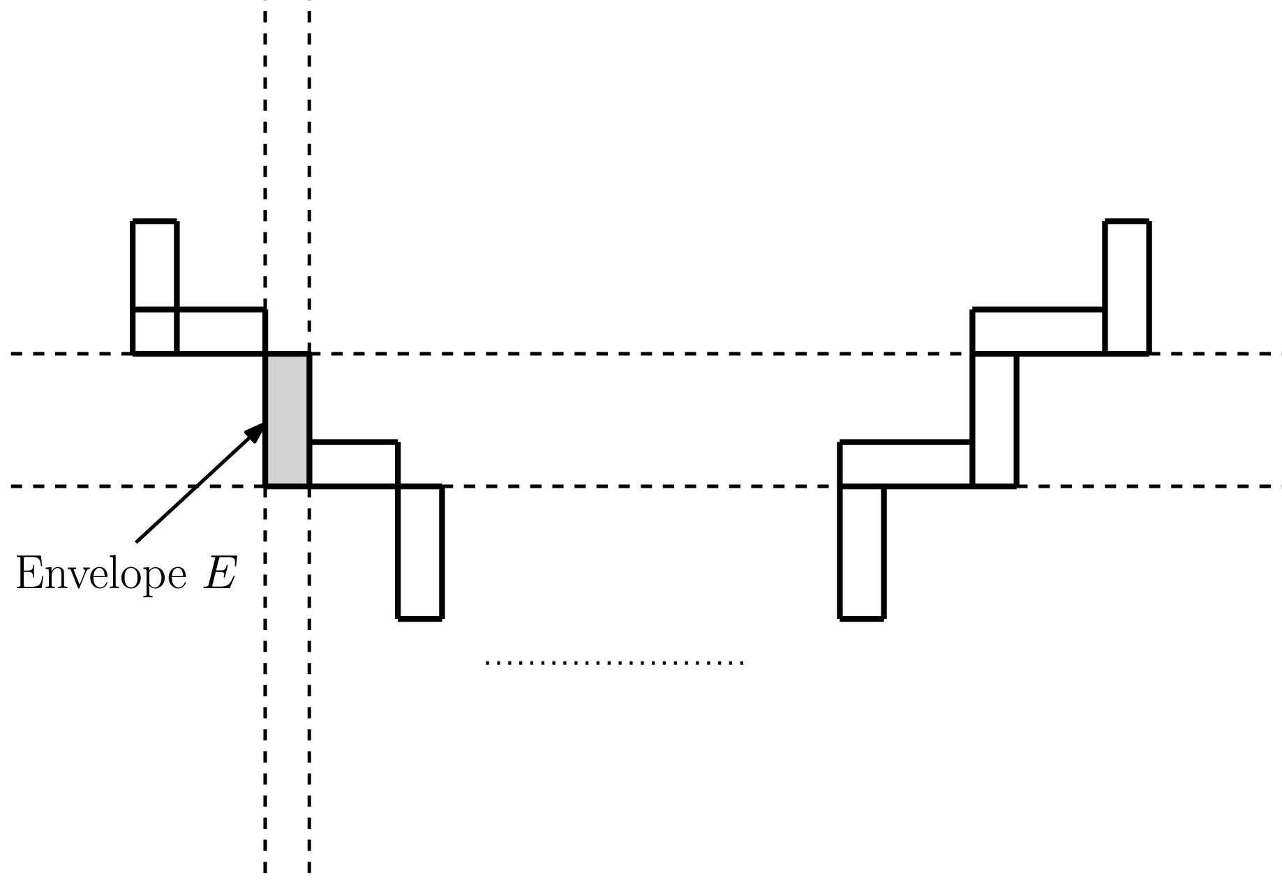
Lemma 4.2. Let
 $S_\ell$
be a skeleton and E the envelope of a step of
 $S_\ell$
. Then
 $\{\tau_{e},e\in E\}$
is independent of
 $\{\tau_{e},e\in E'\}$
for all envelope E′ of
 $S_\ell$
but at most 10 other envelopes E′.
Proof. If the passage times of the edges in an envelope depend on those of E, then this envelope must necessarily touch one of the two strips defined by the sides of E (see Figure 6). Furthermore, based on the construction of our paths and by looking at Figure 6, we can see that there are at most 10 such envelopes.
Envelopes that are dependent on the shaded envelope E.

We are now ready to build
 $\Gamma_\ell$
. It is a random path connecting 0 to x and contained in the set of envelopes of the steps of
 $S_\ell$
. Let
 $\gamma^{\ell}_i$
be the path with the shortest passage time among the two paths connecting
 $x_i^{\ell}$
and
 $x_{i+1}^{\ell}$
in the ith envelope of
 $S_\ell$
. Then we define
 $\Gamma_\ell$
as the concatenation of
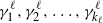 $\gamma^{\ell}_1,\gamma^{\ell}_2,\ldots,\gamma^{\ell}_{k_{\ell}}$
, where
 $k_{\ell}=m_{\ell}+n_{\ell}$
is the number of steps of
 $S_\ell$
. (It is possible that the path
 $\Gamma_\ell$
passes through the same vertex several times.) Notice that the distribution of
 $T(\gamma^{\ell}_{i})$
only depends on the number of edges of the ith step of
 $S_\ell$
. We can then choose
 $\tilde{T}$
such that
 $\tilde{T}\overset{(\mathrm{d})}{=}\min(39\tau_1,\tau_2+39\tau_3+\tau_4)$
. Thus, for all i and
 $\ell$
,
 $\tilde{T}$
stochastically dominates
 $T(\gamma^{\ell}_{i})$
.
Lemma 4.3. For
 $1\leq \ell \leq 3$
and
 $1\leq i\leq k_\ell$
, set
 $T_i^{\ell}=T(\gamma_i^{\ell})$
. Then, for all
 $1\leq k\leq k_\ell$
, there exists
 $C>0$
such that
 $\mathbb{P}\big(\sum_{i=1}^{k}T_{i}^{\ell}>k(\mathbb{E}[\tilde{T}]+1)\big)\leq {C}/{k}$
.
Proof. Using straightforward calculation (see [Reference Auffinger, Damron and Hanson2, (2.3)]) and thanks to Assumption (1.3), for all i and l,
 $\mathrm{Var}(T^\ell_i) < C'$
for some C
′ that does not depend on k, i, and
 $\ell$
. Using Lemma 4.2, we have
 \begin{equation*} \mathrm{Var}\Bigg(\sum_{i=1}^{k}T_i^\ell\Bigg) = \sum_{1\leq i,j\leq k}\mathrm{Cov}(T_i^\ell,T_j^\ell) \leq \sum_{i=1}^{k} 10 \max_j \mathrm{Cov}(T_i^\ell,T_j^\ell). \end{equation*}
Moreover, if
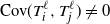 $\mathrm{Cov}(T_i^\ell,T_j^\ell)\neq0$
, then, according to the Cauchy–Schwarz inequality,
 \begin{equation*} |\mathrm{Cov}(T_i^\ell,T_j^\ell)| \leq \sqrt{\text{Var}(T_i^\ell)\text{Var}(T_j^\ell)} \leq C'. \end{equation*}
Consequently,
 $\mathrm{Var}\big(\sum_{i=1}^{k}T_i^\ell\big)\leq 10kC'$
. Thus, since, by definition,
 $\mathbb{E}[\tilde{T}]\geq\mathbb{E}[T_i^\ell]$
for all
 $1\leq i\leq k$
. thanks to the Tchebytchev inequality we have
 \begin{equation*} \mathbb{P}\Bigg(\sum_{i=1}^{k} T_{i}>k(\mathbb{E}[\tilde{T}]+1)\Bigg) \leq \mathbb{P}\Bigg(\sum_{i=1}^{k} T_i^\ell>\sum_{i=1}^{k} \mathbb{E}[T_i^\ell]+k\Bigg) \leq \frac{10}{k}C'. \end{equation*}
Writing
 $C=10C'$
, the result follows.
In order to conclude the proof, we need to control T(0, x) using the independence of
 $\Gamma_1$
,
 $\Gamma_2$
, and
 $\Gamma_3$
. By construction,
 $\Gamma_1$
,
 $\Gamma_2$
, and
 $\Gamma_3$
involve independent envelopes, except in the neighbourhoods of 0,
 $(x_1-x_2,0)$
, and x. In order to exploit this rigorously we introduce some notation:
 \begin{equation*} U_{\ell} = \sum_{i=3}^{m_\ell-2}T_{i}^{\ell} + \sum_{i=m_\ell+3}^{k_\ell-2}T_{i}^{\ell}, \qquad R = \max_{1\leq \ell\leq 3}\Bigg(T_{1}^{\ell}+T_{2}^{\ell} + \sum_{i=m_\ell-1}^{m_\ell+2}T^{\ell}_{i} + T_{k-1}^{\ell} + T_{k}^{\ell}\Bigg). \end{equation*}
We note that in this way, the
 $U_\ell$
are independent. Indeed, by construction, the envelopes of
 $S_\ell$
on which
 $U_\ell$
depends consist of edges located on integer lines distinct from those forming the envelopes of
 $S_\ell'$
on which
 $U_\ell'$
depends, for all distinct
 $\ell,\ell'\in\{1,2,3\}$
. Moreover, thanks to the union bound we have
 $\mathbb{P}(R>\lVert x \rVert_1) \leq 24\mathbb{P}(\tilde{T}>{\lVert x \rVert_1}/{8})$
. Additionally, we notice that
 $T(0,x)\leq R+\min_{1\leq \ell \leq 3}U_{\ell}$
. Therefore, we have with the union bound
 \begin{align*} \mathbb{P}(T(0,x)>(\mathbb{E}[\tilde{T}]+2)\lVert x \rVert_1) & \leq \mathbb{P}(R>\lVert x \rVert_1) + \mathbb{P}\Big(\min_{1\leq \ell\leq 3}U_{\ell}>(\mathbb{E}[\tilde{T}]+1)\lVert x \rVert_1\Big) \\ & \leq 24\mathbb{P}\bigg(\tilde{T}>\frac{\lVert x \rVert_1}{8}\bigg) + \mathbb{P}\Big(\min_{1\leq \ell\leq 3}U_{\ell}>(\mathbb{E}[\tilde{T}]+1)\lVert x \rVert_1\Big). \end{align*}
Now, according to Lemma 4.3,
 $\mathbb{P}(U_{\ell}>k_\ell(\mathbb{E}[\tilde{T}]+1))\leq {C}/{k_\ell}$
. Thus, by the independence of the
 $U_{\ell}$
, we have, since each path is composed of fewer than
 $\lVert x \rVert_1$
steps but more than
 ${\lVert x \rVert_1}/{15}$
,
 \begin{equation*} \mathbb{P}(T(0,x)>(\mathbb{E}[\tilde{T}]+2)\lVert x \rVert_1) \leq 24\mathbb{P}\bigg(\tilde{T}>\frac{\lVert x \rVert_1}{8}\bigg) + (15C)^{3}\lVert x \rVert_1^{-3}. \end{equation*}
Thus, if
 $K=\mathbb{E}[\tilde{T}]+2$
,
 \begin{equation*} \sum_{x\in\mathbb{Z}^2}\mathbb{P}\bigg(\frac{T(0,x)}{\lVert x \rVert_1}>K\bigg) \leq 24\sum_{x\in\mathbb{Z}^2}\mathbb{P}\bigg(\tilde{T}>\frac{\lVert x \rVert_1}{8}\bigg) + (15C)^{3}\sum_{x\in\mathbb{Z}^2}\lVert x \rVert_1^{-3}. \end{equation*}
Thanks to Assumption (1.3),
 $\mathbb{E}[\tilde{T}^d]=\mathbb{E}[\tilde{T}^2]<+\infty$
and so
 $\sum_{x\in\mathbb{Z}^2}\mathbb{P}(\tilde{T}>{\lVert x \rVert_1}/{8})<+\infty$
.
Therefore, since the series of
 $\lVert x \rVert_1^{-3}$
over
 $\mathbb{Z}^{2}$
converges, according to the Borel–Cantelli lemma, there exists
 $\kappa>0$
such that, for all
 $z\in\mathbb{Z}^{2}$
,
 \begin{equation*} \mathbb{P}\bigg(\text{for all }x\in\mathbb{Z}^{2}\setminus \{z\},\, \frac{T(z,x)}{\lVert z-x \rVert_1}<\kappa\bigg)>0. \end{equation*}
Everything we have done here can be generalized in dimension
 $d\geq3$
. Indeed, the biggest difference is that we need to construct
 $d+1$
paths. This construction is achievable by simply spacing out the paths and moving along orthogonal planes to maintain as much independence as possible. Moreover, we then consider d-dimensional envelopes and denote by
 $\gamma_i^\ell$
the path with the shortest passage time among the d paths connecting
 $x_i^\ell$
and
 $x_{i+1}^\ell$
in the ith d-dimensional envelope of
 $S_\ell$
. Thanks to Assumption (1.3), we have in particular
 $\mathbb{E}[\!\min(\tau_1,\ldots,\tau_d)^2]<+\infty$
, so
 $\mathrm{Var}(T_i^\ell)$
are still bounded and, with the obvious notation, we get
 \begin{equation*}\mathbb{P}\Big(\min_{1\leq\ell\leq d+1}U_\ell>(\mathbb{E}[\tilde{T}]+1)\lVert x \rVert_1\Big)\leq C'\lVert x \rVert_1^{-(d+1)}.\end{equation*}
Finally, using that
 $\mathbb{E}[\!\min(\tau_1,\ldots,\tau_d)^d]<+\infty$
, we also get that
 $\sum_{x\in\mathbb{Z}^d}\mathbb{P}(\tilde{T}>{\lVert x \rVert_1}/{8})<+\infty$
.
Proof of Theorem
1.5. We can now use Lemma 4.1 to prove Theorem 1.5 by following the proof in [Reference Auffinger, Damron and Hanson2]. The translation f with vector
 $\zeta\in\mathbb{Z}^d$
is not ergodic when
 $\zeta$
is on one of the axes. However, ergodicity outside the axes is sufficient to prove Theorem 1.5. Indeed, by carefully reading the proof of [Reference Auffinger, Damron and Hanson2, Theorem 2.16], just after formula (2.11), we see that ergodicity along directions arbitrarily close to the axes is sufficient. The result follows.
Proposition 4.1. Assumption (1.3) is necessary for
 $B_t$
to have a limiting shape. More precisely, if
 $\mathbb{E}[\!\min(\tau_{1}^{d},\ldots,\tau_{d}^{d})]=+\infty$
then, for any
 $K>0$
,
 ${T(0,x)}/{\lVert x \rVert_1} > K$
for infinitely many
 $x\in \mathbb{Z}^d$
, a.s.
Proof. Recall that a is the infimum of the support of the distribution of the passage times. Let
 $K>a$
. Let
 $Q=\{z=(z_1,\ldots,z_d)\in\mathbb{N}^d \text{ such that } z_2,\ldots,z_d\leq z_1\}$
. For all
 $z\in Q$
, let
 $A_{z}\,:\!=\,\{\text{for all }i\in [\![ 1,d ]\!], \tau_{z+e_i}\geq dz_1K\}$
. If
 $A_z$
occurs,
 $T(0,z)\geq K\lVert z \rVert_1$
. Then if, for any
 $K>a$
, an infinite number of
 $A_z$
occur, there is no shape theorem. To prove that this is the case with probability 1 if
 $\mathbb{E}[\!\min(\tau_{1}^{d},\ldots,\tau_{d}^{d})]<+\infty$
, we use the following Borel–Cantelli lemma.
Lemma 4.4 ([Reference Erdös and Rényi10, Lemma C]). Let
 $(A_n)_{n\geq1}$
be such that
 $\sum_{n=1}^{+\infty}\mathbb{P}(A_n)=+\infty$
and such that
 \begin{equation*} \limsup_{n\rightarrow+\infty} \frac{\big(\sum_{i=1}^{n}\mathbb{P}(A_i)\big)^{2}}{\sum_{1\leq i,j\leq n}\mathbb{P}(A_i\cap A_j)}=1. \end{equation*}
Then
 $\mathbb{P}({\limsup}\, A_n)=1$
.
In our case, we want to prove that
 \begin{equation*} \limsup_{n\rightarrow+\infty}\frac{\big(\sum_{z\in Q\cap[\![ 1:n ]\!]^d}\mathbb{P}(A_z)\big)^2} {\sum_{z,z'\in Q\cap[\![ 1:n ]\!]^d}\mathbb{P}(A_z\cap A_z')}=1. \end{equation*}
We have
 $\mathbb{P}(A_z)=p_{z_1}^{d}$
, where we put
 $p_i\,:\!=\,\mathbb{P}(\tau\geq dKi)$
. Let
 \begin{equation*} V_n\,:\!=\,\Bigg(\sum_{z\in Q\cap[\![ 1;n ]\!]^{d}}\mathbb{P}(A_z)\Bigg)^{2} = \Bigg(\sum_{i=1}^{n}i^{d-1}p_i^{d}\Bigg)^{2}. \end{equation*}
Now, by assumption,
 $\mathbb{E}[\!\min(\tau_1,\ldots,\tau_d)^{d}]=+\infty$
and by series–integral comparison there exists a constant
 $R>0$
such that
 $\sum_{i=1}^{+\infty}i^{d-1}p_i^{d}\geq R\mathbb{E}[\!\min(\tau_1,\ldots,\tau_d)^{d}]$
. So,
 $\sum_{i=1}^{+\infty}i^{d-1}p_i^{d}=+\infty$
. Let
 $z=(z_1,\ldots,z_d), z'=(z'_1,\ldots,z'_d)\in Q$
and let us write
 $I(z,z')\,:\!=\,\{j\in[\![ 1,d ]\!]\colon z_j=z'_j\}$
. We have
 \begin{equation*} \mathbb{P}(A_z\cap A_{z'}) = \begin{cases} \mathbb{P}(A_z)\mathbb{P}(A_{z'}) & \text{if } |I| = 0, \\ p_{z_1}^{2d-k} & \text{if } |I| = k,\, k > 0,\, 1 \in I, \\[3pt] p_{\min(z_1,z_1')}^{d-k}p_{\max(z_1,z_1')}^{d} & \text{if } |I| = k,\, k > 0,\, 1 \notin I. \end{cases} \end{equation*}
Then
 \begin{align*} \sum_{\substack{z,z'\in Q\cap[\![ 1,n]\!]^{d}}}\mathbb{P}(A_z\cap A_{z'}) & \leq \sum_{\substack{z,z'\in Q\cap [\![ 1,n]\!]^{d}\\|I|=0}}\mathbb{P}(A_z)\mathbb{P}(A_{z'}) + \sum_{k=1}^{d}\sum_{\substack{z,z'\\|I(z,z')|=k\\1\in I(z,z')}}p_{z_1}^{2d-k} \\ & \quad + \sum_{k=1}^{d-1}\sum_{\substack{z,z'\\|I(z,z')|=k\\1\notin I(z,z')}}p_{\max(z_1,z_1')}^{d}p_{\min(z_1,z_1')}^{d-k} \\ & \leq \underbrace{\sum_{\substack{z,z'\in Q\cap [\![ 1,n]\!]^{d}\\|I|=0}} \mathbb{P}(A_z)\mathbb{P}(A_{z'})}_{=:S_{1,n}} + \sum_{k=1}^d 2\binom{d-1}{k-1} \underbrace{\sum_{z_1=1}^n z_1^{2d-k-1}p_{z_1}^{2d-k}}_{=:S_{2,k,n}} \\ & \quad + \sum_{k=1}^{d-1}2\binom{d-1}{k}\underbrace{\sum_{z_1=1}^n z_1^{d-1}p_{z_1}^{d-k} \sum_{z_1'=z_1+1}^nz_1'^{d-k-1} p_{z_1'}^d}_{=:S_{3,k,n}}. \end{align*}
We will now estimate each part of the right-hand side. First, we notice that
 $S_{1,n}\leq V_n$
. Let us first estimate
 $S_{2,k,n}$
for
 $k\in[\![ 1,d ]\!]$
. First, we write
 \begin{equation*} S_{2,k,n}=\sum_{i=1}^{n}i^{2d-k-1}p_i^{2d-k}=\sum_{i=1}^{n}i^{d-1}p_i^{d}(ip_i)^{d-k}. \end{equation*}
Let
 $k\in[\![ 0,d-1 ]\!]$
and
 $i\in\mathbb{N}^{\ast}$
; then there exists a constant
 $C_k>0$
such that

We then have, for all
 $k\in[\![ 0,d-1 ]\!]$
,
 $(ip_i)^{k}\stackrel{i\to+\infty}{=}o\big(\sum_{j=1}^{i}j^{d-1}p_j^{d}\big)$
. It follows that, for all
 $k\in[\![ 1,d ]\!]$
,
 $(ip_i)^{d-k}\stackrel{i\to+\infty}{=}o\big(\sum_{j=1}^{i}j^{d-1}p_j^{d}\big)$
. Since
 $\sum_{j=1}^{i}j^{d-1}p_j^{d}\leq \sum_{j=1}^{n}j^{d-1}p_j^{d}$
, we conclude that, for all
 $k\in [\![ 1,d ]\!]$
,
 $S_{2,k,n}\stackrel{n\to+\infty}{=} o(V_n)$
.
Let us now estimate
 $S_{3,k,n}$
. We see that
 \begin{equation*} S_{3,k,n} = \sum_{i=1}^{n}i^{d-1}p_i^{d-k}\sum_{j=i+1}^{n}j^{d-k-1}p_{j}^{d} = \sum_{j=2}^{n}j^{d-k-1}p_{j}^{d}\sum_{i=1}^{j-1}i^{d-1}p_{i}^{d-k}. \end{equation*}
Now we have

Then, by summing we finally have that, for all
 $k \in [\![ 1,d ]\!]$
,
 $S_{3,k,n}\stackrel{n\to +\infty}{=}o(V_n)$
. To conclude, since
 $S_{1,n}\leq V_n$
and
 $S_{2,k,n}+S_{3,k,n}\stackrel{n\to+\infty}{=} o(V_n)$
, we have
 \begin{equation*} \limsup_{n\rightarrow+\infty}\frac{V_n}{S_{1,n}+S_{2,k,n}+S_{3,k,n}}\geq 1. \end{equation*}
5. Brochette first-passage percolation with infinite passage times
In this section, we allow our passage times to be infinite:
 $\mathbb{P}(\tau=+\infty)>0$
. The proof used here follows the same outline as [Reference Cerf and Théret5], which proved similar results in the context of classical first-passage percolation. The idea in [Reference Cerf and Théret5] was to introduce a regularized notion of passage times. For any
 $M>a$
, we consider the set of edges whose passage time is strictly less than M. The cluster formed by these edges and their endpoints is denoted by
 $\mathcal{C}_M$
. It is easy to see that
 $\mathcal{C}_M$
is infinite, connected, and composed of integer lines. Moreover, we can then define, for all
 $x,y\in\mathbb{Z}^{d}$
,
 $\tilde{T}_{M}(x,y)=T(\tilde{x}_{M},\tilde{y}_{M})$
, where
 $\tilde{x}_{M}$
is the point in the cluster
 $\mathcal{C}_{M}$
closest to x in the
 $L^{1}$
norm with an arbitrary rule to break ties. In the same way, we define
 $\mathcal{C}_\ast$
as the cluster
 $\mathcal{C}_M$
with
 $M=+\infty$
. The proof of Theorem 1.6 is intertwined with that of the following proposition, which shows that
 $\tilde{T}_M$
does not depend on M asymptotically.
Proposition 5.1. For the Brochette first-passage percolation, if
 $\mathbb{P}(\tau<+\infty)>0$
, we have, for all
 $M>a$
, that for all
 $x\in\mathbb{Z}^{d}$
,
 $\lim_{n\rightarrow+\infty}{\tilde{T}_{M}(0,nx)}/{n}=a\lVert x\rVert_1$
a.s. and in
 $L^{1}$
.
To understand and then prove this theorem we now define several objects. If
 $M>a$
, we define the following objects:
-
•
$p_{M}\,:\!=\,\mathbb{P}(\tau\leq M)$
. -
• If
$x,y\in\mathbb{Z}^{d}$
,
$D_{M}(x,y)=\inf\{|\gamma|\colon\gamma\text{ is a path from} \textit{x} \text{to} \textit{y} \text{in }\mathcal{C}_M\}$
is the graph distance in
$\mathcal{C}_M$
, often called the chemical distance between x and y in
$\mathcal{C}_M$
in the context of first-passage percolation. -
•
$D(x,y)=\inf\{|\gamma|\colon\gamma\text{ is a path from}\ \textit{x}\ \text{to}\ \textit{y}\ \text{in}\ \mathcal{C}_\ast\}$
is the chemical distance between x and y in
$\mathcal{C}_\ast$
.







To prove Proposition 5.1, we will once again use Kingman’s subadditive theorem. The only assumption of Kingman’s theorem that is not immediate is the integrability of the process
 $(\tilde{T}_{M}(mx,nx))_{m<n}$
. This is the purpose of our first lemma.
Lemma 5.1. Consider Brochette first-passage percolation. For all
 $M>a$
there exist
 $A_1(M)>0$
and
 $A_2(M)>0$
such that, for all
 $x\in\mathbb{Z}^{d}$
and for all
 $\ell\geq (2d+1)\lVert x \rVert_1$
,
 \begin{equation*} \mathbb{P}(0\leftrightarrow x, D_M(0,x)\geq \ell)\leq A_1(M)\exp({-}A_2(M) \ell). \end{equation*}
Proof. We assume that
 $x=(x_1,\ldots,x_d)$
has all its coordinates positive (the other cases are treated in the same way). Let
 $\ell\geq(2d+1)\lVert x \rVert_1$
. We consider the situation where only one edge emanating from 0 and from x are present, and they are parallel (this is the worst case; the proof is similar and sometimes shorter in other cases). Moreover, to simplify the notation we assume that these edges are
 $\{0,e_1\}$
and
 $\{x,x+e_1\}$
. Define
 $\underline{\ell}\,:\!=\,\lfloor{\ell}/({2d+1})\rfloor$
. If x and y belong to the same integer line
 $\delta$
, we write
 $x\underset{M}{\rightarrow}y$
if the passage time of
 $\delta$
is less than M, i.e. if
 $x,y,\delta\in\mathcal{C}_M$
. Let
 $1\leq c \leq \underline{\ell}$
. We say that
 $(c,0\ldots,0)$
is a good 0-point if the event
 \begin{equation*} (c,0,\ldots,0)\underset{M}{\rightarrow}(c,\underline{\ell},0,\ldots,0)\underset{M}{\rightarrow} (c,\underline{\ell},\underline{\ell},0,\ldots,0)\underset{M}{\rightarrow}\cdots\underset{M}{\rightarrow} (c,\underline{\ell},\ldots,\underline{\ell}) \end{equation*}
occurs. Similarly, if
 $1\leq c' \leq \underline{\ell}$
we say that
 $(c',0,\ldots,0)$
is a good x-point if the event
 \begin{equation*} (c',x_1,\ldots,x_d)\underset{M}{\rightarrow}(c',\underline{\ell},x_3,\ldots,x_d)\underset{M}{\rightarrow} (c,\underline{\ell},\underline{\ell},x_4,\ldots,x_d)\underset{M}{\rightarrow}\cdots\underset{M}{\rightarrow} (c',\underline{\ell},\ldots,\underline{\ell}) \end{equation*}
occurs. The number B of good 0-points and the number B
′ of good x-points follow a binomial distribution with parameters
 $\underline{\ell}$
and
 $p_M^{d-1}$
. Lastly, if we denote by S the set of integers
 $1\leq e \leq \underline{\ell}$
such that
 $(0,\underline{\ell},\ldots,\underline{\ell},e) \rightarrow_{M}(\underline{\ell},\ldots,\underline{\ell},e)$
then its cardinal
 $\tilde{B}$
follows a binomial distribution with parameters
 $\underline{\ell}$
and
 $p_M$
. Moreover, if
 $B,B',\tilde{B}>0$
, then there exists a path connecting 0 to x in
 $\mathcal{C}_M$
with length at most
 $(2d+1)\underline{\ell}\leq \ell$
. We have illustrated the construction in the case of dimension 3 in Figure 7. We leave it to the readers to convince themselves that the construction is similar when the edges emanating from 0 and x are not parallel (see Figure 7b). We can then show that the non-existence of such a path has an exponentially small probability of occurring:
 \begin{align*} \mathbb{P}(0\leftrightarrow x,D_M(0,x)\geq\ell) & \leq \mathbb{P}(0\leftrightarrow x,D_M(0,x)\geq (2d+1)\underline{\ell}) \\ & \leq \mathbb{P}(B=0)+\mathbb{P}(B'=0)+\mathbb{P}(\tilde{B}=0) \\ & \leq 3\mathbb{P}(\tilde{B}=0) \\ & \leq 3\exp(\underline{\ell}\log(1-p_M)) \leq A_1(M)\exp({-}A_2(M)\ell). \end{align*}
Illustration of Lemma 5.1.

Proposition 5.2. There exist three positive constants
 $C_1$
,
 $C_2$
, and
 $C_3$
that depend on M such that, for all
 $x\in\mathbb{Z}^d$
and for all
 $\ell\geq C_3\lVert x \rVert_1$
,
 $\mathbb{P}(\tilde{T}_M(0,x)>\ell)\leq C_1{\mathrm{e}}^{-C_2\ell}$
.
Proof.
 \begin{align*} \mathbb{P}\big(\tilde{T}_M(0,x)>\ell\big) & \leq \mathbb{P}\big(\tilde{0}\notin B_{1}(0,{\varepsilon\ell}/{2})\big) + \mathbb{P}\big(\tilde{x}\notin B_{1}(x,{\varepsilon\ell}/{2})\big) \\ & \quad + \sum_{\substack{a\in B_{1}(0,{\varepsilon\ell}/{2})\cap\mathbb{Z}^{d}\\b\in B_{1}(x,{\varepsilon\ell}/{2})\cap\mathbb{Z}^{d}}} \mathbb{P}\big(\tilde{0}=a,\tilde{x}=b,D_{M}(a,b)\geq{\ell}/{M}\big) \\ & \leq \mathbb{P}\big(\mathcal{C}_{M}\cap B_{1}(0,{\varepsilon\ell}/{2})=\emptyset\big) + \mathbb{P}\big(\mathcal{C}_{M}\cap B_{1}(x,{\varepsilon\ell}/{2})=\emptyset\big) \\ & \quad + \sum_{\substack{a\in B_{1}(0,{\varepsilon\ell}/{2})\cap\mathbb{Z}^{d}\\b\in B_{1}(x,{\varepsilon\ell}/{2})\cap\mathbb{Z}^{d}}} \mathbb{P}\big(a \overset{M}{\longleftrightarrow}b,D_{M}(a,b)\geq{\ell}/{M}\big). \end{align*}
To bound the first two terms, we use the rough estimate
 $\mathbb{P}(\mathcal{C}_{M}\cap B_{1}(0,r)=\emptyset)\leq (1-p_M)^r$
. Moreover, if
 $a\in B_{1}(0,{\varepsilon\ell}/{2})\cap\mathbb{Z}^{d}$
and
 $b\in B_{1}(x,{\varepsilon\ell}/{2})\cap\mathbb{Z}^{d}$
then
 $\lVert a-b \rVert_1\leq \lVert x \rVert_1+\varepsilon \ell.$
Thus, for
 $\varepsilon={1}/{2(2d+1)M}$
and
 $\ell\geq 2M(2d+1)\lVert x \rVert_1$
we can use Lemma 5.1 and we then have
 \begin{equation*} \mathbb{P}\big(\tilde{T}_M(0,x)>\ell\big) \leq 2(1-p_M)^{{\varepsilon\ell}/{2}} + |B_{1}(0,{\varepsilon\ell}/{2})\cap\mathbb{Z}^{d}|^2 A_1\exp({-}A_2\ell). \end{equation*}
Hence the result.
Proof of Proposition
5.1. We first fix
 $M>a$
. All the assumptions of Kingman’s theorem are satisfied, and
 $\tilde{T}_{M}(0,x)$
is integrable thanks to Proposition 5.2. Then we know that
 \begin{equation} \frac{\tilde{T}_{M}(0,nx)}{n}\rightarrow_{n\rightarrow+\infty}X_{M} \quad \text{a.s. and in }L^1, \end{equation}
with
 $X_{M}$
a random variable. However, as in the case where passage times are finite almost surely, the lack of ergodicity implies that, for now, we do not know that the limiting random variable is almost surely equal to a constant. To see that, we study the convergence of a subsequence of
 $({\tilde{T}_{M}(0,nx)}/{n})_{n\geq1}$
in the following lemma.
Lemma 5.2. For all
 $\varepsilon>0$
,
 $x\in \mathbb{Z}^d$
, and
 $M>a$
,
 $a\lVert x \lVert_1 \leq X_{M} \leq M\lVert x \lVert_1$
a.s.
Proof. Let
 $x=(x_1,\ldots,x_d)\in\mathbb{Z}^d$
. By symmetry, we can assume that
 $x_1,\ldots,x_d\geq0$
. By definition, there exists at least one integer line with a passage time less than M passing through
 $\tilde{0}$
. Without loss of generality, assume that the line
 $\tilde{0}+\mathbb{Z}e_1$
has a passage time less than M. Let
 $J=\{n\in\mathbb{N},nx\in\mathcal{C}_M,\,D_M(\tilde{0},nx)\leq\lVert\tilde{0}-nx\rVert_1+2\sqrt{n}\}$
; we show that J is infinite almost surely. If
 $nx\in\mathcal{C}_M$
is such that
 $nx+\mathbb{Z}e_1$
has a passage time less than M, we consider K(n) to be the abscissa of the point in
 $x_1e_1+\mathbb{N} e_1$
closest to
 $x_1$
such that
 \begin{align*} & \tilde{0} + K(n) e_1 \underset{M}{\rightarrow} (\tilde{0}+K(n),x_2,\tilde{0}_3,\ldots,\tilde{0}_d) \underset{M}{\rightarrow}\cdots\underset{M}{\rightarrow} (\tilde{0}+K(n),x_2,\ldots,x_d) \nonumber\\& \qquad \underset{M}{\rightarrow} (x_1,x_2,\ldots,x_d)=x. \end{align*}
Then
 $D_M(\tilde{0},nx)\leq \lVert \tilde{0}-nx\rVert_1+2K(n)$
. K(n) follows a geometric distribution with parameter
 $p\,:\!=\,p_M^{d-1}$
, so
 $\mathbb{P}(K(n)>\sqrt{n})=(1-p)^{\lfloor \sqrt{n}\rfloor}$
. Consequently, by the Borel–Cantelli lemma,
 $K(n)\leq\sqrt{n}$
infinitely often, almost surely. It follows that J is infinite almost surely. Thus,
 \begin{align*} \lim_{n\to+\infty}\frac{\tilde{T}_M(0,nx)}{n} & = \lim_{\substack{n\to+\infty\\ n\in J}}\frac{\tilde{T}_M(0,nx)}{n} \\ & \leq M \liminf_{\substack{n\to+\infty\\ n\in J}}\frac{D_M(\tilde{0},nx)}{n} \\ & \leq M \liminf_{\substack{n\to+\infty\\ n\in J}} \bigg(\frac{\lVert \tilde{0}-0\rVert_1}{n}+\frac{\lVert 0-nx\rVert_1}{n}\bigg) \leq M\lVert x \rVert_1. \end{align*}
Similarly,
 \begin{equation*} \lim_{n\to+\infty}\frac{\tilde{T}_M(0,nx)}{n} \geq \lim_{\substack{n\to+\infty\\ n\in J}}a\frac{D_M(\tilde{0},nx)}{n} \geq a\lim_{\substack{n\to+\infty\\ n\in J}}\frac{\lVert \tilde{0}-nx \rVert_1}{n} = a \lVert x \rVert_1. \end{equation*}
Thus, according to (5.1), if
 $M>a$
we have
 \begin{equation} a\lVert x \rVert_1\leq X_{M}\leq M\lVert x \rVert_1 \quad \text{a.s.}, \end{equation}
as required.
So, we need to show that, in fact,
 $X_{M}$
does not depend on M. To do this, let us fix
 $x\in\mathbb{Z}^d$
. Recall that
 $T^{\ast}(x,y)=T(x^{\ast},y^{\ast})$
where
 $x^{\ast}$
is the closest vertex in the
 $L^{1}$
norm to x in
 $\mathcal{C}_{\ast}$
with an arbitrary rule to break ties. According to the triangle inequality on T,
 \begin{equation*} |T^{\ast}(0,nx)-\tilde{T}_{M}(0,nx)| \leq T(0^\ast,\tilde{0})+T(nx^\ast,\tilde{nx}). \end{equation*}
Since
 $T(0^\ast,\tilde{0})$
and
 $T(nx^\ast,\tilde{nx})$
have same distribution,
 \begin{equation*} \mathbb{P}(|T^{\ast}(0,nx)-\tilde{T}_{M}(0,nx)| \geq \varepsilon n) \leq \mathbb{P}(T(0^\ast,\tilde{0})+T(nx^\ast,\tilde{nx})\geq \varepsilon n) \leq 2\mathbb{P}(T(0^\ast,\tilde{0})\geq {\varepsilon n}/{2}). \end{equation*}
Since
 $0^\ast$
and
 $\tilde{0}$
are both in
 $\mathcal{C}_\ast$
,
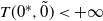 $T(0^\ast,\tilde{0})<+\infty$
and the above inequality implies that
 \begin{equation} \text{for all } x\in \mathbb{Z}^d,\ \frac{T^{\ast}(0,nx)}{n}-\frac{\tilde{T}_M(0,nx)}{n} \overset{\mathbb{P}}{\rightarrow}0. \end{equation}
We can conclude that
 ${T^{\ast}(0,nx)}/{n}$
and
 ${\tilde{T}_M(0,nx)}/{n}$
have the same limit, which cannot depend on M since
 ${T^{\ast}(0,nx)}/{n}$
does not depend on M. By letting M tend to a in (5.2), we deduce that
 \begin{equation} \frac{\tilde{T}_M (0,nx)}{n} \rightarrow_{n \rightarrow + \infty} a \lVert x \rVert_1 \quad \text{a.s.}, \end{equation}
which concludes the proof of Proposition 5.1.

Appendix A
The asymptotic of
 $M_n$
is studied in numerous references, but we have not found any reference regarding the study of
 $\mathbb{E}[M_n]$
. For the sake of self-containedness we provide an estimate of
 $\mathbb{E}[M_n]$
.
Lemma A.1. Assume that the passage times are bounded. Let
 $(\tau_i)_{i\in\mathbb{N}}$
be i.i.d. random variables with cumulative distribution function F such that
 $F(t)\sim_{t\rightarrow 0^{+}}Ct^{\beta}$
for a constant
 $C>0$
and
 $\beta>0$
. Then, if
 $M_n=\min(\tau_1,\ldots,\tau_n)$
, we have
 \begin{equation*} \mathbb{E}[M_{n}] \sim_{n\rightarrow +\infty} \frac{1}{n^{{1}/{\beta}}}\frac{1}{\beta C^{{1}/{\beta}}}\Gamma\bigg(\frac{1}{\beta}\bigg). \end{equation*}
Proof. Let
 $K>0$
be such that
 $\tau\leq K $
almost surely. Writing
 $X_{n}\,:\!=\,M_{n}n^{{1}/{\beta}}$
, we have
 \begin{equation*} \mathbb{E}[X_{n}] = \int_{0}^{+\infty}\mathbb{P}(X_{n}\geq t)\,\mathrm{d}t = \int_{0}^{Kn^{{1}/{\beta}}}\bigg(1-F\bigg(\frac{t}{n^{{1}/{\beta}}}\bigg)\bigg)^{n}\,\mathrm{d}t. \end{equation*}
Now, for a fixed t, we have
 \begin{equation*} \bigg(1-F\bigg(\frac{t}{n^{{1}/{\beta}}}\bigg)\bigg)^{n} = \bigg(1-C\frac{t^{\beta}}{n} + o\bigg(\frac{1}{n}\bigg)\bigg)^{n} \longrightarrow_{n\rightarrow+\infty} \exp({-}Ct^{\beta}). \end{equation*}
Let
 $C'>0$
be such that
 $F(u)\geq C'u^\beta$
for
 $u\in[0, K]$
. Using that
 $(1-{x}/{n})^n\leq {\mathrm{e}}^{-x}$
, we have that, for all
 $t\geq0$
,
 $(1-F({t}/{n^{{1}/{\beta}}}))^n\leq \exp({-}C't^\beta)$
. According to the dominated convergence theorem and with the change of variables
 $u=Ct^{\beta}$
, we have
 \begin{equation*} \mathbb{E}[X_{n}] \rightarrow_{n\rightarrow+\infty} \int_{0}^{+\infty}\exp({-}Ct^{\beta})\,\mathrm{d}t = \Gamma\bigg(\frac{1}{\beta}\bigg) \times \frac{1}{\beta C^{{1}/{\beta}}}. \end{equation*}
So, finally,
 \begin{equation*} \mathbb{E}[M_{n}] \sim_{n\rightarrow+\infty} \frac{1}{n^{{1}/{\beta}}}\frac{1}{\beta C^{{1}/{\beta}}}\Gamma\bigg(\frac{1}{\beta}\bigg). \end{equation*}
Acknowledgements
I would like to warmly thank my two PhD advisors, Anne-Laure Basdevant and Lucas Gerin, first for suggesting this topic and for their support throughout the writing of this article.
Funding information
This work was partially supported by ANR LOUCCOUM.
Competing interests
There were no competing interests to declare which arose during the preparation or publication process of this article.


 Bt
 t=500
 1+Bernoulli(0.95)

 Bt
 t=5
 ne1
 Γ1,Γ2,Γ3