Comparative survey data consist of observations on survey respondents drawn from multiple countries or subnational jurisdictions such as states, provinces or metropolitan areas.Footnote 1 Comparing respondents from different jurisdictions can help to clarify how people differ depending on their social and political contexts, and to test theories about the consequences of macro-social conditions for individuals’ attitudes, beliefs, circumstances and behaviors.
Particularly in the last decade, multilevel models (also known as mixed, random effects or hierarchical linear models) have become a standard method of conducting analyses of this kind. Such models are useful for analyzing observations that are grouped or clustered.Footnote 2 Recent applications to comparative survey data have examined and sought to identify the covariates of outcomes like voting (Gelman et al. Reference Gelman, Park, Shor, Bafumi and Cortina2008), political attitudes (Jamal and Nooruddin Reference Jamal and Nooruddin2010), union membership (Martin and Brady Reference Martin and Brady2007), religiosity (Karakoç and Başkan Reference Karakoç and Başkan2012), health (Jen, Jones and Johnston Reference Jen, Jones and Johnston2009), poverty (Brady, Fullerton and Cross Reference Brady, Fullerton and Cross2009) and gender gaps in household labor (Iversen and Rosenbluth Reference Iversen and Rosenbluth2006). This diversity of applications demonstrates the broad appeal of the method.
Though they find many intriguing cross-sectional associations, very few of these studies address the issue of change over time, and how the kinds of individual-level outcomes cited above may depend on time-varying social, political and economic conditions. This article therefore addresses the question of how to apply multilevel models to survey data that are comparative as well as longitudinal: repeated cross-sectional data, where each cross-section includes a new sample of respondents drawn from the same set of higher-level units. Researchers have access to increasing numbers of datasets of this kind, and a small number of studies has already used multiple waves of data from one or more cross-national surveys that have been fielded multiple times. Yet such studies have generally not made use of the longitudinal character of the data, and—for reasons discussed below—in some cases the approaches that have been used could even be misleading.
This article describes two techniques for analyzing such data and extracting insights about the correlates of change over time; both techniques are simple, incremental extensions of existing multilevel modeling methods. The first is a means of distinguishing between cross-sectional and longitudinal relationships when working with a time-varying, macro-level covariate. Change in y can then be linked to longitudinal variation in some x. The second is the application of “growth curves”—a multilevel modeling technique previously used predominantly with data on individuals—to the level of whole societies. Here, change in y is a function of some time-invariant x.
The article then presents results from a simulation study assessing the performance of these two techniques when applied to data with complications that could occur in real-world applications. Among other things, the simulations show that cross-sectional correlations are biased when a national-level variable is correlated with national-level random intercepts/error terms; the coefficients on the two longitudinal terms proposed here, in contrast, are unbiased—even in the presence of correlated national-level regressors and errors. Further simulations show how statistical power varies with the number of waves of data per country.
Finally, to illustrate the kinds of insights that can be derived using the two techniques, the article applies them to data from the World/European Values Surveys and investigates the relationships between inequality and generalized social trust, and between living standards and postmaterialist values. Previous research has found cross-sectional associations between these pairs of variables; this article tests whether these associations hold longitudinally as well.
The Promise of Extending Multilevel Models Longitudinally
Most existing studies fitting multilevel models to comparative survey data rely exclusively on cross-sectional comparisons, sometimes with few units and thus few degrees of freedom at the higher (country) level. In fact, although the headline conclusions of many such studies rest entirely on comparisons across the higher-level units, in many instances there are fewer than 30 such units, and occasionally fewer than 20.Footnote 3 The results of such cross-sectional comparisons will clearly be sensitive to small changes in either the set of higher-level units or the right-hand-side variables included in the analysis (Beck Reference Beck2007, 97; Wilkes, Guppy and Farris Reference Wilkes, Guppy and Farris2007).Footnote 4
In the context of a theoretical argument about a causal relationship, if a given covariate is cross-sectionally associated with an outcome of interest, checking for the presence of the same relationship longitudinally is a logical next step in validating that the relationship is not spurious. And longitudinal research is a direct way of studying social change in the most general sense—a major task of the social sciences, and a central focus of many specific fields of research.Footnote 5 Currently, however, studies seeking to understand social change often make inferences about longitudinal relationships based on the results of cross-sectional research. Ruiter and van Tubergen (Reference Ruiter and Tubergen2009), for example, derive conclusions about the long-term process of secularization from their cross-sectional study of religious attendance. And on the basis of their cross-sectional study of unionization, Martin and Brady (Reference Martin and Brady2007) argue that when a country signs an agreement with the IMF, there is a decline in the probability that a given resident of that country is a union member. Conclusions about social change based on cross-sectional research are not necessarily wrong, but they are clearly dependent on the ambitious assumption that longitudinal and cross-sectional relationships are the same. As Gelman (Reference Gelman2005, 461) puts it, “it is a big leap to interpret differences between countries as a potential effect of a change within a country.”
The assumption of cross-sectional and longitudinal equivalence will in many instances not be valid. Researchers working with national-level time-series cross-sectional (TSCS) data have found that such data typically fail a standard Hausman (Reference Hausman1978) test of whether cross-sectional and longitudinal relationships are equivalent (Wilson and Butler Reference Wilson and Butler2007). By implication, they are different, and treating them singly will be misleading.
The non-equivalence of cross-sectional and longitudinal relationships has had consequences for the statistical models typically used in analyses of TSCS data. TSCS data can be analyzed using multilevel models in which country-observations are the level-1 units, countries are the level-2 units and level-2 random intercepts are estimated from the data. In practice, however, multilevel models have been used much less than either models estimated using ordinary least square (OLS) with panel-corrected standard errors, or models using fixed effects, which employ country dummy variables instead of random intercepts.Footnote 6 The dummy variables in fixed-effects models hold constant and thus control for differences among countries, though this control comes at the cost that time-invariant country-level variables cannot be included, because the country dummies use up all the degrees of freedom. The fixed-effects approach thus allows for the estimation of only “within” effects, not “between” effects, and cannot test for the correlates of cross-sectional differences across countries.Footnote 7
Recent methodological studies and tests have shown that the few drawbacks of multilevel models for analyzing TSCS data can be relatively easily avoided, however, and such models have several advantages vis-à-vis the fixed-effects approach: “vastly increased flexibility in model specification, potential improvements in model fit, and better accounting of uncertainty at all levels of analysis.”Footnote 8 The possibility of correlation between a time-varying covariate and the country random intercepts is sometimes cited as a reason not to use a multilevel approach, since correlation of this kind will produce a biased estimate of the coefficient on that covariate. But this problem is easily addressed by including the group mean of the time-varying covariate in the model.Footnote 9
Characterizing Comparative Longitudinal Survey Data
This section briefly highlights some key features of comparative longitudinal survey data, and of multilevel models fitted to such data. First, comparative longitudinal survey data are a subcategory of repeated cross-sectional survey data. Comparative survey data allow for comparisons among higher-level units, and respondents included in repeated cross-sectional survey datasets are not necessarily nested in multiple larger macro-level units. A study of repeated cross-sectional survey data in which all respondents are drawn from a single higher-level unit would not be comparative.
Secondly, although societies are by no means reducible to their component members, and survey data are collected on individuals, such data are often sought specifically because they are, in aggregated form, an effective means of measuring differences among societies and of tracking changes in societies over time. But despite the frequency with which survey data are considered in aggregated form, statistical analyses of aggregated data are less informative than those of disaggregated, individual-level data. An analysis based on aggregated data can even be highly misleading, and risks committing an ecological fallacy in which aggregate-level relationships are erroneously assumed also to hold for the individual units on which the pre-aggregated data were collected.Footnote 10 To take one notable recent example, Gelman et al. (Reference Gelman, Park, Shor, Bafumi and Cortina2008) show that voters in American states with higher average incomes have recently tended to vote more for Democratic than Republican candidates. While an analysis using data aggregated to the state level would therefore suggest that Democratic voters tend to be wealthy elites, that is not the case: a multilevel analysis reveals that within states Democratic voters tend to earn lower incomes than Republican voters.
Thirdly, the data drawn from multiple waves of a comparative survey, in which different individual respondents are sampled in each wave, are not generally referred to as panel data; each respondent is observed only once, and panel data are typically defined as data based on repeated observations of the same units. But insofar as societies are units of analysis, and are at least as important as the individuals on which observations are made, then in an important sense the data derived from such surveys are in fact panel data, since societies are each observed multiple times.
Fourthly, macro-comparative social scientists working with quantitative country-level data tend to draw a firm distinction between panel data and TSCS data. There are often just 15 to 20 units observed on repeated occasions in TSCS datasets, whereas typical panel datasets include hundreds or even thousands of units—such as a nationally representative random sample of individuals. Comparative longitudinal survey data are thus non-repeated observations on a large random sample of micro-level units (like panel datasets), and repeated observations on a small non-random sample of macro-level units (like TSCS data).
Existing Models of Comparative Longitudinal Survey Data: De Facto Pooling
This section briefly reviews the approach taken by previous studies in applying multilevel models to comparative longitudinal survey data. A typical two-level multilevel model, in which observations are nested within groups, can be represented as:
 $${\bf {{y}}}\,{\bf {{ = }}}\,{\bf {{X\beta }}}\,{\bf {{ + }}}\,{\bf {{Z\zeta }}}\,{\bf {{ + }}}\,{\bf {{{\epsilon},}}}$$
where y is a vector of outcomes, X is a design matrix comprising a column of ones and columns of covariates, β is a vector of coefficients, Z is a design matrix relating random predictors ζ to the data and ε is a vector of residuals. Unlike the unit dummies in a fixed-effects model, the elements of ζ are not parameters, but random variables conforming to a variance-covariance matrix whose values are parameters that are estimated from the data. A model of this kind, in which individual survey respondents (indexed i) are nested within higher-level societal units (indexed j), and there is one individual- and one group-level covariate, can also be written as:
 $${ & {{y}_{ij}}\, = \,{{\beta }_0}\, + \,{{\beta }_1}{{x}_{ij}}\, + \,{{\beta }_2}{{x}_j}\, + \,{{u}_j}\, + \,{{e}_{ij}},\; \; \; \; \; \; \; \; \; \; \; \; \; \; \; \; \; \; \; \; \; \; \; \; \; \; {\rm for}\,\,i\, = \,1\, \ldots \,{{I}_j},\,j\, = \,1\, \ldots \,J, \cr & {\rm{where}}\,{{u}_j}\, \sim \,{\rm{N}}(0,\,{{\sigma }_u}^{2} )\,{\rm and}\,{{e}_{ij}}\, \sim \,{\rm{N}}(0,\,{{\sigma }_e}^{2} ). \cr}$$
Each j has a random intercept (or group-level disturbance) uj. The x variables can be either variable across individuals within countries (subscripted ij) or invariant within but variable across countries (j). Some representations of multilevel models prefer to use a series of two or more equations (one at each level), and this article adopts such an approach below, where useful.
Aside from normally distributed data, multilevel models have long been extended to generalized linear models with binary, count, proportion, etc. outcomes (including event history or survival analysis), using a variety of estimation techniques and link functions.
Among the few previous studies that have incorporated multiple waves of comparative survey data, the dominant approach has been to fit a three-level model in which respondents (i) are nested within country-years (tj), which in turn are nested within countries (j). Such a model can include a coefficient capturing the effect on y of an x variable that varies both across countries and within countries over time. This x variable is considered to be a characteristic of country-years, and is indexed tj, because it is constant for individuals within a given country-year, and non-constant across both countries and the country-years nested within a given country:
 $$ {{{y}_{itj}}\, = \,{{\beta }_0}\, + \,{{\beta }_1}{{x}_{itj}}\, + \,{{\beta }_2}{{x}_{tj}}\, + \,{{u}_j}\, + \,{{u}_{tj}}\, + \,{{e}_{itj}}, \cr {\rm{where}}\,e_{itj}\, \sim \,{\rm{ N}}(0,{}{{\sigma }_e}^{2} ),\,{{u}_{tj}}\, \sim \,{\rm{N}}(0,\,{{\sigma }_{u1}}^{2} ),\,\,{\rm{and}}\,{{u}_j}\, \sim \,{\rm{N}}(0,\,{{\sigma }_{u2}}^{2} ).$$
Jen, Jones and Johnston (Reference Jen, Jones and Johnston2009) adopt this approach, for example, in their test of Wilkinson and Pickett's (Reference Wilkinson and Pickett2006, Reference Wilkinson and Pickett2009) hypothesis that societal-level income inequality tends to lead people to have poorer health. Contrary to multilevel analyses of individuals nested in US states,Footnote 11 they find that across countries, inequality does not correlate with poorer health. Solt (Reference Solt2008) uses the same approach to study the effect of inequality on political engagement.Footnote 12
This approach investigates social change only in the limited sense that, by using all the available survey data, those data happen to have a longitudinal dimension. Though the x variable of interest varies both over time and across countries, these two dimensions of its variability are treated singly—making it impossible to know whether a single dimension is driving any covariation found with y, or even (potentially) whether the two associations have different signs. This approach effectively assumes that the cross-sectional and longitudinal relationships between x and y are the same: a single coefficient β linked to xtj captures both. That assumption of equivalence, as discussed earlier, will often be unjustified.
Distinguishing Between Cross-Sectional and Longitudinal Relationships
I now turn to extensions of existing multilevel modeling techniques that address the limitations of existing approaches. The first extension I describe allows for the simultaneous but separate analysis of cross-sectional and longitudinal relationships. The technical requirement for distinguishing between cross-sectional and longitudinal relationships is simple: calculating a mean, and subtracting that mean from the time-varying variable of interest xtj. The technique thus group-mean centers the covariate.Footnote 13
Separate longitudinal and cross-sectional associations between xtj and y can be identified by calculating the mean of xtj across all relevant years for each country. The coefficient on the country mean  $$${{\bar{x}}_j}$$$
captures the effect on y of enduring cross-national differences in xtj. To capture the effect on y of variation over time within each country,
 $$$ {{\bar{x}}_j} $$$
can then be subtracted from xtj. The resulting longitudinal component xtjM (a country-year level variable) is group-mean centered, and is orthogonal to
 $$${{\bar{x}}_j}$$$
, such that the two coefficients can be estimated separately.Footnote 14 The resulting model is:
 $${{y}_{itj}}\, = \,{{\beta }_0}\, + \,{{\beta }_1}{{x}_{itj}}\, + \,{{\beta }_2}{{x}_{tjM}}\, + \,{{\beta }_3}{{\bar x}_{{\square}j}}\, + \,{{\beta }_4}tim{{e}_{tj}}\, + \,{{u}_j}\, + \,{{u}_{tj}}\, + \,{{e}_{itj}}.$$
The original variable xtj is thus entered twice, having been decomposed into  $$${{\bar{x}}_j}$$$
and xtjM. Binary variables can be treated the same as continuous ones; the group mean simply becomes a proportion (Enders and Tofighi Reference Enders and Tofighi2007). The equation also includes a variable for time—this could be a set of year dummies and/or a linear effect, and could also include a quadratic term. The need for a time term arises from the possibility of simultaneous but unrelated time trends in both xtj/xtjM and y. If both are increasing over time, including a control for time reveals whether y tends to grow faster for units experiencing a faster increase in x.
This extension, which allows for both “between” and “within” effects, represents an important improvement on existing techniques: it provides a direct investigation of social change without assuming that the longitudinal relationship is the same as the cross-sectional one. This extension investigates the possible covariation between a shift in x over time and a shift in y over time. This relationship can be investigated even as the cross-sectional association between  $$${{\bar{x}}_j}$$$
and y is also estimated. Note that time-varying national-level variables can be the national average of a particular individual characteristic (for example, education or social capital).
There are precursors to this extension. Previous studies and commentaries have remarked on the benefits of group-mean centering when fitting multilevel models.Footnote 15 As mentioned earlier, Bafumi and Gelman (Reference Bafumi and Gelman2006) note that group-mean centering provides a simple resolution of concerns about correlations between one or more regressors and the random effects, or equivalently the higher-level errors. Bartels (Reference Bartels2008) cited the benefits of country-mean centering in analyses of national-level TSCS data. And Moller, Alderson and Nielsen (Reference Moller, Alderson and Nielsen2009) use group-mean centering to analyze the drivers of cross-sectional and longitudinal variations in US counties’ levels of inequality. The author has recently applied this technique in a study with US states as the macro-level unit (Fairbrother and Martin Reference Fairbrother and Martin2013), but otherwise its usefulness for analyses of comparative longitudinal survey data has not previously been noted.
Societal Growth Curves
The technique introduced in the previous section investigates the association between a shift in xtj over time and a shift in y over time. But it does not investigate whether the absolute level of some time-invariant (continuous or categorical) variable xj leads to faster or slower change in y. Yet one would ideally want to test for such patterns, and this section introduces a technique for doing so: the application of “growth-curve modeling” to the higher-level units in comparative longitudinal survey data. An xj variable of interest in this regard could be the country mean  $$${{\bar{x}}_j}$$$
discussed above, though it could also denote some other time-invariant macro-level characteristic, such as the share of a jurisdiction's territory located in the tropics, the identity of a country's former colonial ruler or the type of welfare state regime.
“Growth curves,” which entail multilevel models of measurement occasions nested within individuals, have long been applied to individual-level panel data such as in psychology or education research.Footnote 16 Canonically, growth-curve analyses have been used in studies of child or adolescent development, and have answered questions about how a feature y, such as performance on a test of mental or physical ability, changes as subjects age. Such models allow for the possibility that change in y over time varies not with change in x, but according to the fixed level of x—for example gender or some characteristic of an individual's family or home environment in his/her early years.
Mathematically, just as distinguishing between cross-sectional and longitudinal effects involves no more than a simple decomposition, growth curves require only an interaction between an xj variable and time.Footnote 17 A growth curve can be represented using equations at two levels as:
 $${{y}_{tj}}\, = \,{{\beta }_{0j}}\, + \,{{\beta }_{1j}}tim{{e}_{tj}}\, + \,{{e}_{tj}}{\rm{,}}$$
where ytj represents j's score at time t (t = 1 … T), timetj is a time-varying (continuous or categorical) variable indexing time for individual j, and β0j and β1j represent a random intercept and time slope, respectively, for j. This is the level-1 equation. The intercept and slope parameters are random effects, which can vary across units, as indicated by their j subscripts. Two level-2 equations describing these parameters are then:
 $${ & {{\beta }_{0j}}\, = \,{{\gamma }_{00}}\, + \,{{\gamma }_{01}}{{x}_{1j}}\, + \,{{\gamma }_{02}}{{x}_{2tj}}\, + \,{{u}_{0j}}, \cr & {{\beta }_{1j}}\, = \,{{\gamma }_{10}}\, + \,{{\gamma }_{11}}{{x}_{3j}}\, + \,{{u}_{1j}}\,\,\,\,{\rm{and}} \cr & etj\, \sim \,{\rm{N}}(0,\,{{\sigma }_e}^{2} ),\,{{u}_{0j}}\, \sim \,{\rm{N}}(0,\,{{\sigma }_{uo}}^{2} ),\,\,{\rm{and}}\,\,{{u}_{1j}}\, \sim \,{\rm{N}}(0,\,{{\sigma }_{u1}}^{2} ){\rm{.}} \cr}$$
In the level-2 equations, the intercept term β 0j combines an overall intercept γ 00, time-invariant and time-varying covariates x 1j and x 2tj (with coefficients γ 01 and γ 02 respectively), and a random intercept unique to each j, denoted as u 0j. Similarly, the time slope β 1j is the sum of an overall slope γ 10, a time-constant covariate x 3j with coefficient γ 11 and a j-specific random disturbance u 1j. The covariance of the random intercepts and slopes may be estimated. The special capability of the growth-curve model is that it allows for the modeling of time (β 1j) as a function of one or more time-invariant covariate(s) of interest; the rate of change over time depends on time-invariant predictors (Collins Reference Collins2006). Growth “curves” are often curvilinear (with quadratic functions of time or orthogonal polynomials), but can also be linear or discrete. The challenge of this technique can be interpretation, since the statistical significance of interaction effects depends on how covariates are entered, and can be subject to weak statistical power (Mathieu et al. Reference Mathieu, Aguinis, Culpepper and Chen2012).Footnote 18
For analyses of comparative longitudinal survey data, I propose the use of “societal growth curves”—a growth curve at the societal level rather than the individual level.Footnote 19 Since societies are observed multiple times in repeated cross-sectional survey data, the pattern of change of each one over time can be described using a curved or straight line. A societal growth curve illustrates the pattern of change over time—the rate of change and the height of the original starting point. Such an approach has recently been used to good effect by Poznyak, Abts and Swyngedouw (Reference Poznyak, Abts and Swyngedouw2011), who investigate the characteristics of regions in Belgium where support for the far right has been rising faster than elsewhere.
How can growth-curve analysis be applied to whole societies, where observations on those societies are collected via observations on individuals? A societal growth-curve model fitted to repeated cross-sectional individual-level survey data can be specified as:
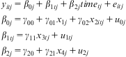 $${{{y}_{itj}}\, = \,{{\beta }_{0j}}\, + \,{{\beta }_{1tj}}\, + \,{{\beta }_{2j}}tim{{e}_{tj}}\, + \,{{e}_{itj}} \cr {{\beta }_{0j}}\, = \,{{\gamma }_{00}}\, + \,{{\gamma }_{01}}{{x}_{1j}}\, + \,{{\gamma }_{02}}{{x}_{2itj}}\, + \,{{u}_{0j}} \cr {{\beta }_{1tj}}\, = \,{{\gamma }_{11}}{{x}_{3tj}}\, + \,{{u}_{1tj}} \cr {{\beta }_{2j}}\, = \,{{\gamma }_{20}}\, + \,{{\gamma }_{21}}{{x}_{4j}}\, + \,{{u}_{2j}} \\ $$
Here γ 00 refers to the overall intercept, γ 01 denotes the fixed effect of country-level covariate x 1j, γ 02 denotes the fixed effect of individual-level covariate x 2itj and u 0j is a country j-specific random intercept. In the second of the stage-2 equations, γ 11 refers to the fixed effect of a country-year level variable x 3tj and u 1tj is a country-year level random intercept. In the third of the stage-2 equations, γ 20 denotes the fixed effect for time (the average time slope across all units), γ 21 the effect of a time-invariant country-level covariate x 4j on the time slope and u 2j the random disturbance for each country j. Thus the outcome y for individual i in country j observed at time t is the sum of an intercept; fixed effects at the country, country-year and individual levels; random intercepts for countries and country-years; an individual-level disturbance; and the effect of time— comprising an overall trend, a country-level fixed effect and a country-level random disturbance.
Where there are concerns that a series may be non-stationary, time series in x can be tested for stationarity using techniques for panel unit root tests.Footnote 20 The possible non-stationarity of y can be checked using the same techniques but applied to the ij random intercepts from a null model. The simulations that follow also address concerns about autocorrelation.Footnote 21
Simulation Study
This section reports the results of simulations assessing the performance of the above two techniques, including for data exhibiting a variety of complications that could be present in real-world applications. For a series of eight data-generating processes, I investigate the bias and efficiency of the parameter estimates and the optimism of the fixed effects’ standard errors (SEs); optimism is defined by Shor et al. (Reference Shor, Bafumi, Keele and Park2007) as the ratio of the true sampling variability to the estimate of the variability provided by the SEs. I generate the data in R and fit the models with the “lme4” package (Bates, Maechler and Bolker Reference Bates, Maechler and Bolker2012), using restricted maximum likelihood, or maximum likelihood with a Laplace approximation when estimating binomial models, as described further below. The base data-generating process (DGP 1) is:
 $${ & {{y}_{itj}}\, = \,{{\beta }_0}\, + \,{{\beta }_1}{{{\bar{x}}}_j}\, + \,{{\beta }_2}{{x}_{tjM}}\, + \,{{\beta }_3}{{x}_{itj}}\, + \,{{\beta }_4}tim{{e}_{tj}}\, + \,{{\beta }_5}tim{{e}_{tj}}\ast\,{{{\bar{x}}}_j}\, + \,{{u}_j}\, + \,{{u}_{tj}}\, + \,{{e}_{itj}}{\rm{,}} \cr & {\rm{with}}\,uj\, \sim \,{\rm{N}}(0,\,{{\sigma }_{u1}}^{2} ),\,{{u}_{tj}}\, \sim \,{\rm{N}}(0,\,{{\sigma }_{u2}}^{2} ),\,\,{\rm{and}}\,\,{{e}_{itj}}\, \sim \,{\rm{N}}(0,\,{{\sigma }_e}^{2} ). \cr}$$
The time-varying covariate xtj has a random time trend, and is partitioned into  $$${{\bar{x}}_j}$$$
and xtjM. The idea is to mimic a national-level variable, such as gross domestic product (GDP) per capita or the Gini index for income inequality. The xitj variable is a binary individual-level covariate. The intercept and the coefficients on
 $$${{\bar{x}}_j}$$$
, xtjM and timetj*
 $$${{\bar{x}}_j}$$$
are set to 1, and those on xitj and timetj to −1.Footnote 22 The random effects variances are set at 2 for countries, 1 for country-waves and 9 for the residual term—yielding variance shares that are roughly typical of real-world applications.
Each simulated dataset has 12,500 “respondents” nested in 25 “countries.” To investigate any impacts of having just a few waves of observations per country, I “observe” 2, 5 or 20 randomly selected years out of a 30-year range; each country-year includes 250, 100 or 25 people, respectively, yielding a total of 500 observations per country in all cases.Footnote 23 The R code used to conduct these simulations is available as in the online appendix, and can be easily modified to test many different variations: different sizes of N at different levels, combinations of complications, different effect sizes, random effects variances, etc. For each DGP and combination of Ns, I simulated and fit a model to 1,000 datasets. Seven subsequent data-generating processes each modify DGP 1 as follows:
2. The country random intercepts uj are correlated with
 $$${{\bar{x}}_j}$$$
. Such correlation could arise, for example, from endogeneity or omitted variables.Footnote 24 The results in this case should be of particular interest, given the prevalence of cross-sectional multilevel analyses in which the greatest interest is in the coefficient on some xj. The covariance is set at 0.7 (for uj with variance 2, and
$$${{\bar{x}}_j}$$$
with variance 1, such that the correlation is 0.49).
3. The country random intercepts uj are correlated with xitj. Since xitj is an individual-level binary variable, the correlation is created between uj and the country mean of xitj (that is, the probability of each “respondent” having xitj = 1). The covariance is set at 0.7 between uj and the mean national xitj on the logit scale.
4. The country-wave intercepts utj are temporally autocorrelated. The autocorrelated utj are generated before country-waves are selected at random for “observation,” such that the autocorrelation across successive observed years within a country will vary. The autocorrelation is set at 0.25 between units one lag apart.
5. The country random intercepts uj are non-normally distributed, whereas typically multilevel models, as here, are fitted on the assumption that the random intercepts are normally distributed. In this DGP, they are distributed skew-normally (using the “sn” package by Azzalini Reference Azzalini2011).
6. The effects of xtjM are lagged by five years, and the fitted model assumes no lag. Such a model misspecification is a real concern, since theory may provide very little guidance as to the timescale on which effects will be felt.
7. The probability of a country-wave's selection (from the range of possible country-waves) is positively related to the value of xtj. Probability weights are proportional to the antilogit of xtj, and a fixed number of country-waves per country are drawn.
8. The dependent variable is binary rather than normal. The model is therefore fit as a generalized linear mixed model with an antilogit link. To speed up convergence, “respondents” in the same country-waves with the same covariates (at all levels) are binned, yielding a shortened dataset with many Bernoulli trials per row rather than just one. A model fitted this way yields the same fixed and random effects parameter estimates as one in which responses are not binned (Subramanian et al. 2001).


Figures 1 through 3 present the results of the simulation study. In all three, within each of the eight data-generating processes, the results are presented from left to right for simulations with two, five and 20 country-waves per country (represented by Os, dots and Xs, respectively).
Figures 1 and 2 plot the mean and 95 percent coverage intervals of the estimated fixed effects coefficients and random effects variances, with the true value indicated by a horizontal line. (Fixed effects whose true values are -1 have had their sign reversed for presentation.)
Means and 95 percent coverage intervals for each beta coefficient
Note: derived from the simulations described in the text, for each of eight data-generating processes. Os, dots and Xs are for simulations with, respectively, two and 250, five and 100, and 20 and 25 waves per country and respondents per country-wave. True values are all 1.

Means and 95 percent coverage intervals for each random effect variance
Note: Os, dots and Xs are for simulations with, respectively, two and 250, five and 100, and 20 and 25 waves per country and respondents per country-wave. True values are shown with a horizontal line.
Figure 1 shows that the fixed effects coefficients are unbiased, except for the coefficient on  $$${{\bar{x}}_j}$$$
where
 $$${{\bar{x}}_j}$$$
is correlated with uj (DGP 2), and the intercept where the effects of xtjM are lagged and the fitted model assumes no lag (DGP 6). In the latter instance, further simulations (not reported) indicate that the magnitude of the bias on the intercept varies positively with the magnitude of the effect of xtjM. If data are generated with both the correlation in DGP 2 and the lag of DGP 6, the biases are combined but do not multiply each other. The variances of the coefficient estimates differ substantially across coefficients, given the different variances of the covariates, but not across DGPs. Observing more waves per country, for a fixed number of observations per country, yields tighter estimates of the coefficients on all variables except xitj. Observing even just five rather than two country-waves per country has substantial benefits for precision.
In Figure 2, the random effects variances are generally unbiased, with the exception that the country-level variance is downward biased for DGP 2, and to a lesser extent for DGP 8 (a binomial outcome). The dispersal of a fixed number of observations per country across a larger number of country-waves yields tighter estimates of the variances of the country-wave and country random intercepts.
Figure 3 plots the “optimism” of the SEs returned for the fixed effects coefficients. The estimated SEs for all six coefficients in most scenarios reflect the true variability of the estimates—the optimism is close to 1. In some cases, the SEs are slightly too large (over-conservative) or too small (anti-conservative). The scenario in which the SEs are most misleading is DGP 4, where country-wave intercepts utj are temporally autocorrelated, though there is only a problem if the number of country-waves is large. The SEs here are substantially too small for the coefficients on Time, the time-varying xtjM and the interaction between Time and  $$${{\bar{x}}_j}$$$
. There is thus some risk of committing a Type 1 error if countries are observed at many points in time and there may be autocorrelation.
Optimism of the SEs returned in the simulation study
Note: calculated as in Shor et al. Reference Shor, Bafumi, Keele and Park2007. Values above one indicate anti-conservative SEs, while values below derive from SEs that are over-conservative. Os, dots and Xs are for simulations with, respectively, two and 250, five and 100, and 20 and 25 waves per country and respondents per country-wave.
Overall, then, with a little caution in interpreting the significance tests, these techniques appear relatively robust to real-world complications. Concerns about potentially inaccurate SEs could be further addressed using Markov chain Monte Carlo (MCMC) estimation, or in a maximum likelihood context with a bootstrap or other resampling technique.Footnote 25
One final concern is statistical power, and the risk of committing a Type 2 error if the number of country-waves observed per country is small.Footnote 26Figure 4 reports the results of additional simulations, similar to DGP 1 described above, but estimated using MCMC and setting the true coefficient on xtjM to 0, 0.25, 0.5, 0.75 or 1.Footnote 27 Where it is 1, the effects of  $$${{\bar{x}}_j}$$$
and xtjM are the same. Figure 4 therefore contrasts the results obtained using group-mean centering (and estimating both
 $$${{\bar{x}}_j}$$$
and xtjM) with those obtained by estimating xtj alone.
Proportion of estimated 95 percent highest posterior density intervals that exclude 0 (top row) and mean estimates of the fixed effects coefficients (bottom row)
Note: derived from simulations with true xtjM ranging from 0 to 1. De facto pooling yields estimates for xtj (left column) and mean centering for  $$${{\bar{x}}_j}$$$
and xtjM (center and right columns). Os, dots and Xs are for simulations with, respectively, two and 250, five and 100, and 20 and 25 waves per country and respondents per country-wave.
Figure 4 shows that the number of country-waves observed per country strongly influences the risk of a Type 2 error, above all for the coefficient on xtjM but also to a lesser extent for the coefficient on  $$${{\bar{x}}_j}$$$
. In some cases, the pooled effect of xtj is more likely to be statistically significant than the partitioned effects of xtjM and
 $$${{\bar{x}}_j}$$$
. But the bottom row of Figure 4 also shows how the mean estimate of the coefficient on xtj varies with the number of country-waves per country, and represents a hard-to-interpret combination of xtj's two component parts (Raudenbush and Bryk Reference Raudenbush and Bryk2002, 138). Where the true effect of xtjM is 0, the coefficient on xtj will often be statistically significant, without clarifying that only the cross-sectional component is driving the overall effect. In this sense, there is no simple solution to the problem of weak power if the number of country-waves is small; applied researchers will need to be careful not to over-interpret a statistically non-significant coefficient on xtjM.
Applications
This section applies the techniques described above to analyze World/European Values Survey data on two topics. Across five waves (which spanned from 1981 to 2008, depending on the country), these surveys included 445,319 individuals in 97 countries and 245 country-waves (countries have been observed in one to five waves, with developing and non-democratic countries noticeably less well represented).
Some samples were not drawn in ways that would make them nationally representative. Consequently, I follow Stevenson and Wolfers (Reference Stevenson and Wolfers2008) in excluding 17 country-waves from the first four waves, and using the same criteria I also exclude respondents surveyed in one country (Chile) in the fifth wave. These exclusions leave fewer than 97 countries and 245 country-waves, as specified below.Footnote 28
Trust
The first topic is generalized social trust—that is, trust in a “generalized other” rather than a known relative, friend or acquaintance. The literature regards trusting citizens as desirable: they tend to be more socially and politically engaged, generous in their charitable giving, tolerant and happy with their lives, while countries with more trusting populations enjoy faster economic growth, better governance and lower crime (Rothstein and Uslaner Reference Rothstein and Uslaner2005, 41; Bjørnskov Reference Bjørnskov2008, 271).
A number of previous studies has linked trust to equality, on the theoretical grounds that people tend to be more trusting of people similar to them, and inequality reduces the share of the population to whom a given person is similar (Uslaner Reference Uslaner2002; Bjørnskov Reference Bjørnskov2008). Empirically, in support of this theory, previous work has emphasized negative correlations between inequality and trust across nations (Bjørnskov Reference Bjørnskov2008; Freitag and Bühlmann Reference Freitag and Bühlmann2009; Knack and Keefer Reference Knack and Keefer1997; Rothstein and Uslaner Reference Rothstein and Uslaner2005; Uslaner Reference Uslaner2002, Reference Uslaner2008). Largely on the strength of such cross-sectional correlations, the existing literature presents inequality as “arguably the strongest determinant of the level of social trust.”Footnote 29 Uslaner (Reference Uslaner2002, 186) argues boldly that “the level of economic inequality is the prime mover of generalized trust.” Yet Fairbrother and Martin (Reference Fairbrother and Martin2013) find only a cross-sectional (but no longitudinal) relationship between inequality and trust across US states, and no relationship of either kind for US counties.
I further test the evidence for inequality as a major influence on people's trust in generalized others at the international level. For measuring trust, the relevant WVS/EVS question (A165) is: “Generally speaking, would you say that most people can be trusted or that you can't be too careful in dealing with people?” This question has been validated using cross-national differences in the prevalence of trusting behavior in experimental contexts (Johnson and Mislin Reference Johnson and Mislin2012) and by experimentally “losing” wallets in public places and counting the proportion returned to their “owners” (Knack and Keefer Reference Knack and Keefer1997). In both cases, the proportion of self-reported trusters in a country correlates with observation-based measures of trusting behavior.
For data on the time-varying level of inequality in a country, I use Solt's (Reference Solt2009) Standardized World Income Inequality Database, version 3.0, which is based on data from the UN but improves on direct estimates of inequality using a custom missing-data algorithm to make observations more comparable to each other.
Figure 5 plots self-reported trust against income inequality, aggregating individual data for all possible countries and waves (except non-representative samples, as explained earlier). Visually, slopes of the logistic regression lines suggest negative associations between inequality and trust both cross-sectionally and longitudinally, though the cross-sectional relationship (in the left panel) is clearer than the longitudinal relationship (center panel). Moreover, the slope of the line in the center panel could be a product of simultaneous but unrelated declines in both equality and trust over time. The right panel shows that trust has indeed been declining over time, and at roughly the same rate in nations with mean levels of inequality (pooling across waves) that are lower or higher than the median of countries’ mean levels of inequality. The techniques proposed here test whether the inequality-trust link holds longitudinally when controlling for time and for the clustering of observations within countries and country-years.
Mean level of trust Versus inequality (first two panels) or time (right panel), with a single-level logistic regression line
Note: the clustering of country-waves within countries is ignored. In the right panel, crosses and dots denote observations from countries with less or more than median country-mean inequality, respectively, and the two lines are fit separately for these two groups of countries.
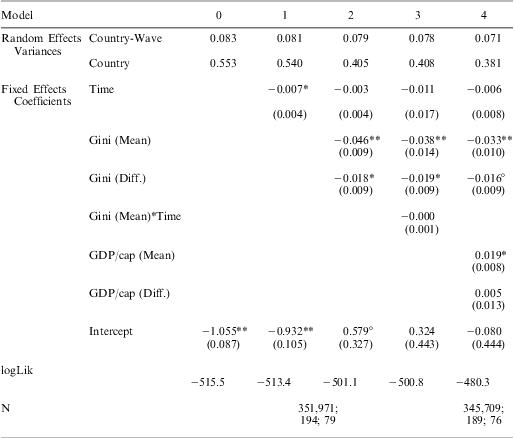
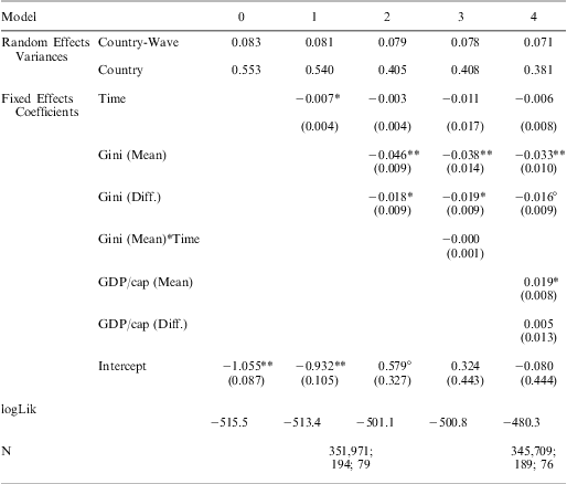
The model used here investigates the log-odds of a “Most people can be trusted” response as opposed to a “Can't be too careful” response. “Don't know” responses were dropped. A logit model was estimated via maximum likelihood and the Laplace approximation. Table 1 presents the model results. Model 0 is a null model with no covariates other than a constant, while Models 1 through 3 add covariates and Model 4 includes controls for GDP/capita.
Logistic Multilevel Models of Trust
Note: SEs in parentheses. Ns are for respondents, country-waves and countries.
**< 0.01, *p < 0.05, °p < 0.1.
The main findings are that, across all specifications, the coefficient on Gini (mean) is negative and statistically significant at the 0.01 level, while the coefficient on Gini (differenced) is slightly less robust but still also generally negative and statistically significant. In contrast, the coefficient on the growth-curve term is not statistically significant in any specification. The variance for the country random intercepts declines substantially with the inclusion of covariates at the country level, while the variance of the country-wave random intercepts shrinks slightly with the addition of the longitudinal (differenced) component of Gini.
The coefficient on the longitudinal component of Gini is only statistically significant at the 0.1 level if a random slope for time is included (with or without estimating a covariance between the random slope and the random country intercepts). A likelihood ratio test, however, suggests the random slopes are not warranted. In Model 4, if GDP per capita is entered in logged form, the coefficient on the mean component is no longer statistically significant, though other results are substantively similar, and the model fit is inferior.
These results are therefore consistent with claims of a link between inequality and trust.Footnote 30 In countries where inequality has increased over time in recent decades, people have become systematically less trusting.
Postmaterialist Values
As the living standards of a country's residents rise to the extent that most people's basic material needs are met, do their priorities shift to non-economic, higher-order concerns—about equality, self-determination, freedom and quality of life? In articulating a theory that they do, Inglehart coined the concept of “postmaterialist” values, arguing that growing material affluence and security lead to more tolerant, egalitarian, participatory and nurturing societies.Footnote 31
To measure people's possession of postmaterialist versus materialist values, the World/European Values Surveys include an index (Y002) reflecting respondents’ answers to a two-part question (E003 and E004): “If you had to choose, which one of the things on this card would you say is most important? And which would be the next most important?” The options are: “Maintaining order in the nation,” “Give people more say,” “Fighting rising prices” and “Protecting freedom of speech.” Respondents who named “Give people more say” and “Protecting freedom of speech” were coded as “postmaterialists,” while those who chose the other two options were coded as “materialists.” Respondents who selected one of each pair (in either order) were coded as “mixed.” The postmaterialist values index therefore has three (ordinal) response categories.
The hypothesis has come under criticism, such as from Davis and Davenport (Reference Davis and Davenport1999), who say that postmaterialist values are “virtually unexplainable as a dependent variable.” Clarke and Dutt (Reference Clarke and Dutt1991) and Clarke, Dutt and Rapkin (Reference Clarke, Dutt and Rapkin1997) contend that the postmaterialist-materialist index is too sensitive to current economic conditions and not to the more slow-changing conditions hypothesized by the concept's defenders to be more important. There has also been much debate about the appropriate level of analysis in studies of postmaterialist versus materialist values,Footnote 32 with critics of the index's usefulness generally preferring individual-level research and advocates favoring aggregate-level research.
Here I link responses to the postmaterialism index to real GDP per capita (at purchasing power parity), as provided by the World Bank's World Development Indicators. Figure 6 plots postmaterialist values against GDP per capita in the same two ways as Figure 5 for trust and inequality. Again, the cross-sectional relationship is clear, with a strongly upward-sloping line showing the relationship between average living standards and postmaterialist values. In the center panel, the line is also upward sloping, albeit less steep, and in the right panel postmaterialist values appear to be growing in prevalence in wealthier (but not poorer) nations.
Mean level of postmaterialist values Versus GDP per capita (first two panels) or time (right panel), with a linear regression line
Note: the clustering of country-waves within countries is ignored. In the right panel, crosses and dots denote observations from countries with less or more than median country-mean GDP per capita, respectively, and the two lines are fit separately for these two groups of countries.
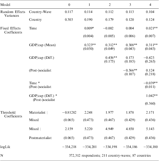
A cumulative link/ordered logit model was estimated via maximum likelihood and the Laplace approximation, using the R “ordinal” package (Christensen Reference Christensen2012).Footnote 33Table 2 presents the results. Model 2 suggests there are statistically significant cross-sectional and longitudinal associations between national standards of living (GDP per capita) and the probability of postmaterialist versus materialist values. But robustness checks revealed that the inclusion of a dummy variable for being a (post-)socialist nation makes this relationship much weaker, and no longer statistically significant at even the 0.1 level (Model 3).Footnote 34 However, Model 4 clarifies with an interaction term that the longitudinal relationship is quite strong for (post-)socialist nations, while not significant for others. Moreover, as indicated by the other interaction term, the underlying growth curve for the two groups of countries differs substantially: ceteris paribus, postmaterialist values are declining for (post-)socialist countries, but increasing in others. In other models (not reported), the growth-curve coefficient for all countries taken together is not significant.
Cumulative (Logit) Link Multilevel Models of Postmaterialist Values
Note: SEs in parentheses. GDP/capita is entered in logged form, though main results also hold if it is not logged.**< 0.01, *p < 0.05, °p < 0.1
These results therefore provide mixed support for the theory of postmaterialist values. Specifically, in the context of the rapid social change of the transition from state socialism to capitalism, differences in processes of economic development appear to have had important consequences for people's values. But these results also suggest that in many contexts, there is little relationship between development and postmaterialist values, even if the cross-sectional relationship is strong and consistent.
Conclusions
The applications presented here, using statistical models embodying a multilevel view of repeated observations of nations, have shown how comparative longitudinal survey data can be used to test hypotheses about the consequences of both time-varying and time-invariant macro-social conditions. The evidence for longitudinal relationships between inequality and generalized social trust, and between economic growth and postmaterialist values, represents important extensions and tests for the literatures on these topics.
Across the social sciences, a typical goal of much research is to explain social change. Repeated cross-sectional survey data would appear to be a natural tool for this work, and to some extent such data are already being put to use. However, existing applications do not fully exploit the properties of such datasets, and risk overlooking—or even deriving misleading inferences about—key relationships. Comparative longitudinal survey datasets should be a valuable resource for research on political and social change in the broadest sense; they should help answer big questions about why and how societies change, and why some change faster than others. Because of the increasing availability of these kinds of datasets, the usefulness of the techniques described here should only increase over time.