



1. Introduction and main results
From a single sprout to an entire forest, plant growth has long inspired mathematical models in ecology (see, e.g., [Reference Barril, Calsina, Diekmann and Farkas4, Reference Barril, Calsina, Diekmann and Farkas5, Reference Bessonov and Volpert8, Reference Callaway10, Reference Hasik, Kopfová, Nábělková and Trofimchuk19, Reference Magal and Zhang27]). Among the factors shaping forest dynamics is the size-based hierarchy of trees: taller trees, advantaged in photosynthesis, dominate smaller ones. This hierarchical structure naturally lends itself to the theory of physiologically structured populations (see [Reference Magal and Zhang27, Reference Metz and Diekmann29, Reference Smith30, Reference Webb33]). A recent example is a phenomenological forest model structured by height, formulated in [Reference Barril, Calsina, Diekmann and Farkas4, Reference Barril, Calsina, Diekmann and Farkas5] as a renewal equation
 \begin{equation}
b(t) =\int_0^\infty \beta\left( x_m + \int_0^a g\left( e^{-\mu(\tau -a)} \int_a^\infty e^{-\mu s}b(t-s)ds\right)d\tau \right) e^{-\mu a}b(t-a)da,
\end{equation}
where  $b(t)$ is the tree’s population birth rate at time
 $t$,
 $g(x)$ denotes the growth rate of an individual of height
 $x$, the positive parameter
 $\mu \gt 0$ represents the per capita death rate, and
 $\beta(x)$ is the per capita reproduction rate (depending only on height
 $x$). It is assumed that all newborn individuals have the minimal height
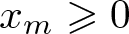 $x_m\geqslant0$.
Model (1.1) is in close agreement with the classical partial differential equation (PDE) formulation obtained via a conservation law [Reference Barril, Calsina, Diekmann and Farkas4]. More precisely, the height-structured population density 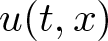 $u(t,x)$ satisfies the nonlinear conservation law
 \begin{equation}
\partial_t u(t,x)+\partial_x\!\big(g(E(t,x))u(t,x)\big)+\mu u(t,x)=0,\quad x \gt x_m,\ t \gt 0,
\end{equation}
with the nonlocal boundary condition
 \begin{equation*}
g(E(t,x_m))u(t,x_m)=\int_{x_m}^{\infty}\beta(x)u(t,x)\,dx,
\quad
E(t,x)=\int_x^{\infty}u(t,y)\,dy.
\end{equation*}
The PDE formulation (1.2), derived in [Reference Barril, Calsina, Diekmann and Farkas4, Reference Barril, Calsina, Diekmann and Farkas5], is equivalent to the renewal equation (1.1) at the modelling level; however, the renewal formulation leads to a scalar functional equation for the birth rate, which is better suited for the analysis of long-time behaviour. In particular, as pointed out in [Reference Barril, Calsina, Diekmann and Farkas4, Reference Barril, Calsina, Diekmann and Farkas5], the applicability of a principle of linearized stability to the PDE formulation (1.2) remains an open issue. We refer to [Reference Barril, Calsina, Diekmann and Farkas4, Reference Barril, Calsina, Diekmann and Farkas5] for more details and further discussion.
Note that first-order PDEs with nonlinear and nonlocal boundary conditions—such as the Gurtin–MacCamy age-structured model [Reference Ducrot, Kang and Magal15, Reference Gurtin and MacCamy18, Reference Magal and Ruan26, Reference Webb33]—can be analysed by reducing them to nonlinear integral equations. For instance, as shown in [Reference Herrera and Trofimchuk21, Reference Ma and Magal25], by integrating along characteristics, the essential dynamics of the system
 \begin{equation}
\begin{cases}
(\partial_t + \partial_a)u(t,a) = -\mu u(t,a), & t \gt 0,~ a \gt 0 \\
u(t,0) = f\left( \int_0^\infty \gamma(a)u(t,a)\,da \right)\!, & t \gt 0, \quad u(0,\cdot)=u_0\in L^1(\mathbb{R}_+),
\end{cases}
\end{equation}
where  $f: \mathbb{R}_+ \to \mathbb{R}_+$ is a bounded continuous function and
 $\beta(a):= \gamma(a)e^{-\mu a}$ is integrable on
 $\mathbb{R}_+$, can be captured by the convolution equation
 \begin{equation}
\xi(t) = \int_0^\infty \beta(a) f(\xi(t-a))da, \ t \in \mathbb{R}.
\end{equation}
The dynamics of the nonlinear equation (1.4) has been the subject of numerous studies; see [Reference Amster, Hasík, Kopfová and Trofimchuk1, Reference Asselah and Nussbaum2, Reference Breda, Diekmann, Liessi and Scarabel9, Reference Chow, Diekmann and Mallet-Paret12–Reference Diekmann and van Gils14, Reference Griette and Herrera16, Reference Gripenberg, Londen and Staffans17, Reference Hasik, Kopfová and Trofimchuk20, Reference Herrera and Trofimchuk21, Reference Ma and Magal25, Reference Metz and Diekmann29] and the references therein. A key structural feature of equation (1.4) is that its kernel  $\beta$ is independent of the state variable
 $\xi$, while the nonlinearity
 $f$ is bounded (typically monotone or unimodal). In contrast, equation (1.1) possesses a more complex structure, as its kernel is coupled to a linear unbounded term and depends on the state in a nontrivial manner.
A direct computation shows that if  $\beta(u)\equiv\beta(x_m)$ is constant in equation (1.1), then all admissible positive solutions are unbounded on
 $\mathbb{R}_+$ whenever
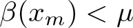
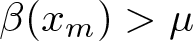 $\beta(x_m) \gt \mu$, whereas they converge to zero if
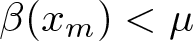 $\beta(x_m) \lt \mu$. Hence, the state dependence of the kernel in (1.1) enables a feedback tuning of the solution dynamics that is absent in the classical convolution setting.
The analysis of equation (1.1) thus provides an important step toward a deeper understanding of renewal equations with state-dependent structure and the associated quasi-linear, non-local first-order PDE models. In this paper, we adapt an approach developed in [Reference Herrera and Trofimchuk21] for the convolution equation (1.4) in order to investigate the stability and persistence properties of the more complex equation (1.1) via an associated one-dimensional dynamical system. In doing so, we complement the functional-analytic method of [Reference Diekmann and Gyllenberg13], which was previously applied in [Reference Barril, Calsina, Diekmann and Farkas4, Reference Barril, Calsina, Diekmann and Farkas5] to equation (1.1) under rather strong monotonicity conditions
(M) Mappings
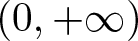
 $\beta:[x_m,+\infty)\to [0, +\infty)$,
$g: [0,+\infty)\to (0, +\infty)$ are continuous,
$\beta$ is strictly increasing, and
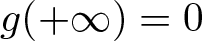
$g$ is strictly decreasing one with
$g(+\infty)=0$.




Remark 1. It is worth noting here that for many tree species, the fertility function  $\beta$ generally increases with height, as larger individuals tend to have greater access to light and reproductive resources. However, the assumption that the fertility function
 $\beta$ is everywhere non-decreasing may be biologically unrealistic. In some species, excessive height can adversely affect seed viability due to ecological and physiological mechanisms such as resource allocation trade-offs, pollen limitation, increased rates of autonomous self-pollination, or senescence-related effects [Reference Caraballo-Ortiz, Santiago-Valentín and Carlo11]. These considerations emphasize the biological relevance of per capita reproduction rates
 $\beta$ that display a hump-shaped (unimodal) dependence on height. Further discussion and a number of open problems are presented in Section 4.
We now define the following function, which will be used throughout the paper:
 \begin{equation}
R(b):=\int_0^\infty
\beta\!\left(
x_m+\int_0^a g\!\left(\frac{e^{-\mu\tau}}{\mu}\,b\right)\,d\tau
\right)e^{-\mu a}\,da.
\end{equation}
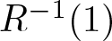
If (M) holds, then  $R(b)$ is strictly decreasing and, in particular,
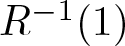 $R^{-1}(1)$ is either empty or a singleton; in the latter case, it will be denoted by
 $b_*$.
As in [Reference Barril, Calsina, Diekmann and Farkas4, Reference Barril, Calsina, Diekmann and Farkas5], we view (1.1) as an integral equation with infinite memory and a nonnegative initial history  $b(s)=\phi(s)\geqslant0$ for
 $s \lt 0$. Even for continuous
 $\phi$, the solution
 $b(t)$ may have a jump at
 $t=0$, which motivates working in the positive cone
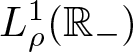
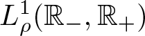
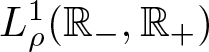 $L^1_\rho(\mathbb{R}_-,\mathbb{R}_+)$ of a Banach space of measurable functions
 \begin{equation*}
L^1_\rho(\mathbb{R}_{-})= \{\phi: |\phi|_\rho \lt \infty\}, \quad \mbox{where we use the notation} \quad |\phi|_q:= \int_{-\infty}^0|\phi(s)|e^{qs}ds,
\end{equation*}
with 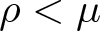 $\rho \lt \mu$, as the phase space for (1.1) instead of spaces of continuous functions of fading-memory type [Reference Atkinson and Haddock3].
By introducing the nonlinear functional  $\mathfrak{F}: L^1_\rho(\mathbb{R}_{-}, \mathbb{R}_+) \to \mathbb{R}_+$ defined by
 \begin{equation}
\mathfrak{F} \phi:=\int_0^\infty \beta\left( x_m + \int_0^a g\left( e^{-\mu(\tau -a)} \int_a^\infty e^{-\mu s} \phi(-s)\,ds \right) d\tau \right) e^{-\mu a} \phi(-a)da,
\end{equation}
we get the abstract form  $\phi(t)=\frak F\phi_t, \ \phi_t \in L^1_\rho(\mathbb{R}_{-}, \mathbb{R}_{+})$ of equation (1.1). Here the standard notation
 $\phi_t(s)=\phi(t+s), \ s \lt 0$, is used.
Fixing an initial function  $\phi\geqslant0$, we can also rewrite equation (1.1) in the Volterra’s form
 $b(t) = (\mathcal{V}_\phi b)(t) + r_\phi(t)$, where
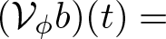 $(\mathcal{V}_\phi b)(t) =$
 \begin{equation*}
\int_0^t \beta\left( x_m + \int_0^a g\left( e^{-\mu(\tau -a)}\left(\int_a^t e^{-\mu s} b(t-s)ds+ e^{-\mu t}|\phi|_\mu\right)\right)d\tau\right) e^{-\mu a}b(t-a)da,
\end{equation*}
 \begin{equation*}
r_\phi(t)= \int_t^\infty \beta\left( x_m + \int_0^a g\left( e^{-\mu(\tau -a)} \int_a^\infty e^{-\mu s} \phi(t-s)ds\right) d\tau \right) e^{-\mu a} \phi(t-a)da.
\end{equation*}
Then a standard argumentation (outlined in Appendix) yields the following existence, uniqueness and eventual positivity result.
Proposition 1. Assume that  $\beta:[x_m,\infty)\to[0,\infty)$ is continuous with at most polynomial growth, and that
 $g:[0,\infty)\to[0,\infty)$ is continuous and bounded. Then
(a) there exists at least one non-negative function
$b_\phi(t)$ which is continuous on
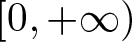
$[0, +\infty)$ and solves the initial value problem
$\textstyle b(s)=\phi(s)\geqslant 0,\;s \lt 0$ for (1.1);(b) in addition, if
$\beta$ is a locally Lipschitzian function, then the solution
$b_\phi$ is a unique one, it is continuously differentiable on
$(0,+\infty)$ and the derivative
$b_\phi'(t)$ is a bounded function on each interval
$(0,T]$.(c) Moreover, if the assumption of item (b) is satisfied and
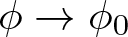
$\phi \to \phi_0$ in
$L^1_\rho(\mathbb{R}_{-}, \mathbb{R}_{+})$, then
$b_\phi(t) \to b_{\phi_0}(t)$ uniformly on compact subsets of
$[0,+\infty)$.(d) Furthermore, if
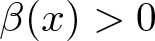
$\beta(x) \gt 0$ a.e. on
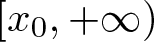
$[x_0,+\infty)$ for some
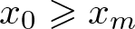
$x_0\geqslant x_m$ and
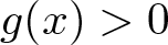
$g(x) \gt 0$ for all
$x\geqslant0$, then either
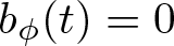
$b_\phi(t) =0$ for all
$t \in \mathbb{R}$ or there exists some
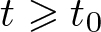
$t_0=t_0(\phi)\geqslant0$ such that
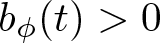
$b_\phi(t) \gt 0$ for all
$t\geqslant t_0$.

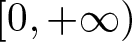









By relaxing assumptions of growth and continuity on  $\beta$ and
 $g$, Proposition 1 improves [Reference Barril, Calsina, Diekmann and Farkas5, Theorem 2] and shows that if
 $\beta$ is polynomially bounded and locally Lipschitzian, then the renewal equation (1.1) generates a continuous semiflow
 \begin{equation*}\mathcal F:L_\rho^1({\mathbb{R}}_-,{\mathbb{R}}_+)\times{\mathbb{R}}_+\rightarrow L_\rho^1({\mathbb{R}}_-,{\mathbb{R}}_+)\quad\text{by}\;(\mathcal F^t\phi)(s)=b_\phi(t+s),\;s\leqslant0.\end{equation*}
It has a zero steady state 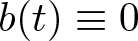 $b(t) \equiv 0$ while the positive equilibria of this semiflow coincide with the positive equilibria of a one-dimensional system
 $b_{n+1}= \frak F b_n$
 $=: F(b_n) , \ b_n \gt 0$. Since
 $F(b)=bR(b)$, where
 $R(b)$ is given by (1.5), these positive equilibria are determined by the scalar equation
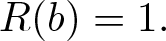 $R(b)=1.$ As we already noted, under hypothesis (M) function
 $R(b)$ is strictly decreasing on
 $\mathbb{R}_+$ and the latter equation has a unique positive solution
 $b_*$ if and only if
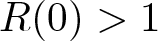 $R(0) \gt 1$ and
 $R(+\infty)= \beta(x_m)/\mu \lt 1$, cf. [Reference Barril, Calsina, Diekmann and Farkas5, Theorem 4]. A straightforward application of the comparison argument shows that all solutions of equation (1.1) are exponentially converging to
 $0$ when
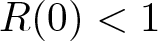 $R(0) \lt 1$, see Theorem 6 in [Reference Barril, Calsina, Diekmann and Farkas5] (as we show it later, under hypothesis (M), all solutions vanish at
 $+\infty$ even if
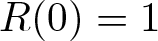 $R(0)=1$). Thus, if (M) is assumed, then
 $R(0)$ can be interpreted as the basic reproduction number.
Assume now that equation (1.1) has a positive equilibrium  $b_*$ (e.g.,
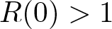 $R(0) \gt 1$,
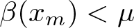 $\beta(x_m) \lt \mu$). One of the basic questions concerns its stability properties with respect to the semiflow
 $\mathcal F^t \phi$. Using the principle of linearized stability for delay equations from [Reference Diekmann and Gyllenberg13], the authors of [Reference Barril, Calsina, Diekmann and Farkas4] proved the local asymptotical stability of the positive equilibrium
 $b_*$ for the particular case of bounded functions
 $g$ and
 $
\beta(x)=\max\{0,x-x_A\},
$ where
 $x_A \gt x_m=0$ denotes the adult size at which reproduction begins, (see Theorem 5.4 in [Reference Barril, Calsina, Diekmann and Farkas4]). Note that their approach required certain technical efforts while establishing the continuous differentiability of the operator
 ${\frak F}: L^1_\rho(\mathbb{R}_{-}, \mathbb{R}) \to \mathbb{R}$.
Clearly, local asymptotic stability of the positive equilibrium does not preclude more complex dynamics (e.g., periodic or unbounded trajectories) of the semiflow  $\mathcal F^t \phi$. This question was not considered in [Reference Barril, Calsina, Diekmann and Farkas4, Reference Barril, Calsina, Diekmann and Farkas5], and it is the main object of study in the present work. Here we show how stability and persistence properties of a scalar nonlinear renewal equation
 $\phi(t)=\frak F\phi_t, \ \phi_t \in L^1_\rho(\mathbb{R}_{-},\mathbb{R}_{+})$, can be efficiently established through analysis of the induced one-dimensional system
 $b_{n+1}= \frak F b_n, \ b \in \mathbb{R}_+$. This allows us to describe the general structure of the semiflow
 $\mathcal F^t \phi$ under relatively weak assumptions on functions
 $\beta$ and
 $g$. In our next result, the monotonicity assumption (M) is not required; however, as in [Reference Barril, Calsina, Diekmann and Farkas4], we assume that
 $\beta:[x_m,+\infty)\to [0, +\infty)$ is globally Lipschitz.
Theorem 2. Assume that  $\textstyle0\leqslant\beta(x_m) \lt \;\mu$,
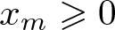 $x_m\geqslant0$,
 $R(0) \gt 1$, that
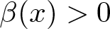 $\beta(x) \gt 0$ a.e. on
 $[x_0,+\infty)$ for some
 $x_0\geqslant x_m$, that
 $\beta$ satisfies the global Lipschitz condition on
 $\mathbb{R}_+$ and that positive continuous function
 $g$ vanishes at
 $+\infty$. Then on the open set
 $L^1_\rho(\mathbb{R}_{-}, \mathbb{R}_+)\setminus \{0\}$, the semiflow
 $\mathcal F^t \phi$ has a compact global attractor
 $\mathcal A$ attracting each solution with initial datum in
 $L^1_\rho(\mathbb{R}_{-}, \mathbb{R}_+)\setminus \{0\}$. Furthermore, restricted to any compact interval
 $[-n,0] \subset \mathbb{R}_-$,
 $n \in \mathbb{N}$, this convergence is uniform in the sup-norm. Next, each element of
 $\mathcal A$ is a differentiable function, and there are universal positive numbers
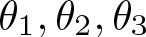 $\theta_1, \theta_2, \theta_3$ such that
 \begin{equation*}
0 \lt \theta_1 \leqslant \psi(s) \leqslant \theta_2, \quad |\psi'(s)| \leqslant \theta_3, \ s \leqslant 0, \ \mbox{for each} \ \psi \in \mathcal A.
\end{equation*}
In particular, by establishing strong permanence properties of the semiflow  $\mathcal F^t \phi$, this result supports the qualitative validity and biological consistency of model (1.1). An explicit (constructive) upper bound
 $\theta_2$ for
 $\mathcal A$ in the sup-norm is given in Corollary 4. According to the classification of global attractors in [Reference Smith and Thieme32, Chapter 2], the compact set
 $\mathcal A$ in Theorem 2 is a global attractor of points. In view of the possibility of complete positive orbits connecting the zero equilibrium and
 $\mathcal A$, this attractor does not attract every bounded set. Thus,
 $\mathcal F^t \phi$ restricted to the open subset
 $L^1_\rho(\mathbb{R}_{-}, \mathbb{R}_+)\setminus \{0\}$ of the phase space
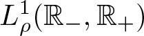 $L^1_\rho(\mathbb{R}_{-}, \mathbb{R}_+)$ is not asymptotically smooth, cf. [Reference Smith and Thieme32, Theorem 2.33]. Still, as the next theorem shows,
 $\mathcal A$ can be a compact attractor of neighbourhoods of compact sets, cf. [Reference Magal and Zhao28, Reference Smith and Thieme32]. In the next theorem, we describe the structure of the global attractor
 $\mathcal A$, assuming the hypothesis
(M*) Mappings
$\beta:[x_m,+\infty)\to [0, +\infty)$,
$g: [0,+\infty)\to (0, +\infty)$ are continuous,
$g(\infty)=0$,
$\beta$ is non-decreasing and has at most polynomial growth. Moreover, the function
$R(b)$ defined in (1.5) satisfies the property that its preimage
$R^{-1}(1)$ is either empty or consists of a single point
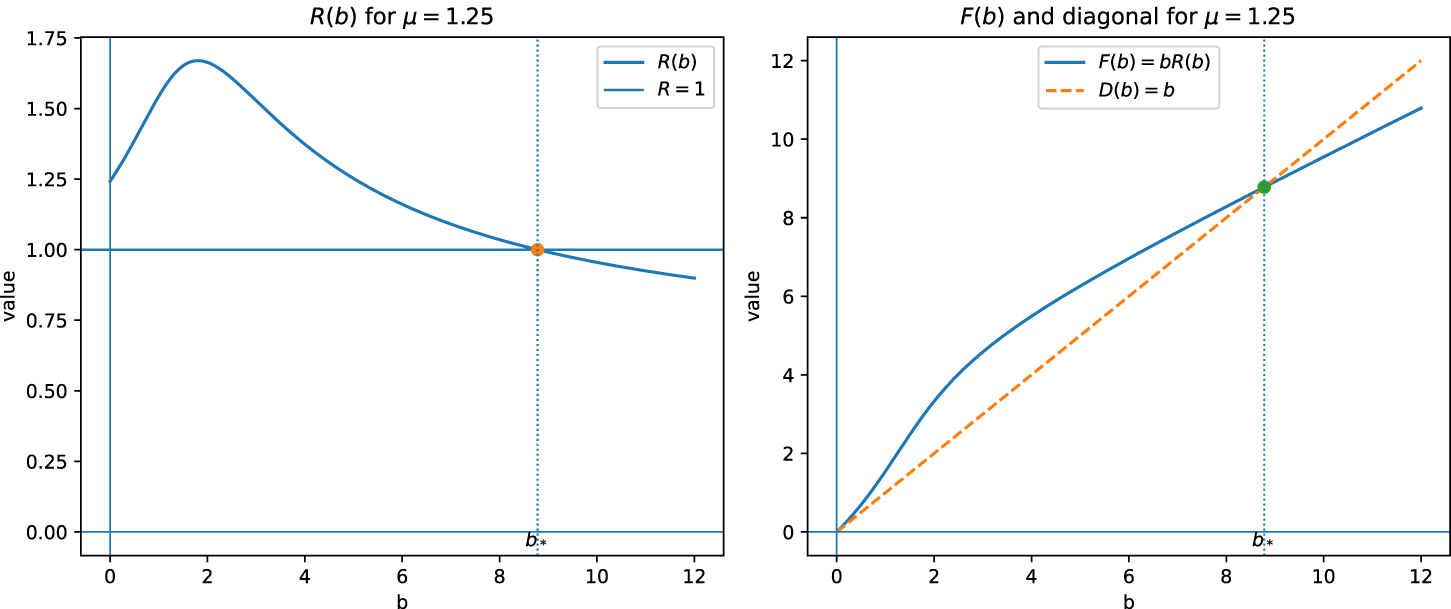
$b_*$, as shown in Figure 1.
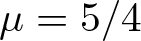
Figure 1.Graphs of
$R(b)= \frac{3}{5} + \frac{8}{5b} \left( \arctan\left( \frac{4}{5}b - 1 \right) + \frac{\pi}{4} \right)$ (left panel) and
$F(b)=bR(b)$ (right panel) corresponding to the choice of
$\beta(u)=u+3/4$,
$g(x)=2/(1+(x-1)^2)$, and
$\mu=5/4$. In this case, the function
$R(b)$ is non-monotone, while
$F(b)$ is strictly increasing.











Remark 3. Note that (M*) is weaker than (M), since it allows for non-monotone functions  $g$, thereby extending the range of applicability of the model (1.4). Indeed, following [Reference Barril, Calsina, Diekmann and Farkas5], the height of an individual tree is assumed to evolve according to the equation
 $x'(t)=g(E)$, where
 $E=E(t,x)$ denotes the number of trees whose height is at least
 $x$ at time
 $t$. If growth is limited solely by light availability, then an increase in
 $E$ cannot improve the local light conditions. In this case, it is natural to assume, as in (M), that
 $g(E)$ is a decreasing function.
However, in certain ecological settings, it is reasonable to regard  $E$ as a proxy for a more complex environment mediated by taller individuals. Such individuals may reduce wind stress, stabilize humidity, and temperature, or provide photoprotection and mechanical support, thereby enhancing the growth of shorter individuals at low values of
 $E$; for larger values of
 $E$, shading effects become dominant, and growth is reduced. This mechanism naturally leads to unimodal growth functions
 $g(E)$; see, for example, [Reference Callaway10, Chapter 2, xeric habitat in Figure 2.2]. Thus, instead of describing hierarchical competition solely through growth reduction as in [Reference Barril, Calsina, Diekmann and Farkas5], the present framework allows one to capture both hierarchical competition and facilitation via non-monotone shape of the individual growth function.
Theorem 4. Assume that  $\mu \gt 0,x_m\geqslant0$, that
 $\beta$ is a globally Lipschitzian function, and that the assumption (M*) is satisfied. Then
(i) If
$b_*$ uniquely solves
$F(b)=b$ on
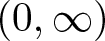
$(0,\infty)$ and
$\beta(x_m) \lt \mu$, then the equilibrium
$b_*$ attracts all non-zero solutions and is locally stable in the uniform norm: i. e. for each
$\epsilon \gt 0$ there exists
$\delta \gt 0$ such that each solution
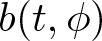
$b(t,\phi)$ of the initial value problem
$b(s,\phi)=\phi(s),\;s \lt 0,$ satisfies
$|b(t,\phi)-b_*| \lt \epsilon$,
$t\geqslant0$, once
$|\phi- b_*|_\rho \lt \delta$. Moreover, if
$\delta \gt 0$ is sufficiently small, then
$\lim_{t \to +\infty}|b(t,\phi)-b_*|=0$ uniformly on the open ball
$|\phi- b_*|_\rho \lt \delta$. In particular,
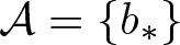
$\mathcal A= \{b_*\}$ attracts neighbourhoods of compact sets in
$L^1_\rho(\mathbb{R}_{-}, \mathbb{R}_+)\setminus \{0\}$.(ii) If equation
$F(b)=b$ does not have positive solutions and
$F'(0)=R(0) \gt 1$, then each non-zero solution to equation (1.1) is unbounded;(iii) If
$F(x) \lt x$,
$x \gt 0$, then each solution to ( 1.1) vanishes at
$+\infty$.
















The key fact in the proof of this theorem is that (M*) implies the monotonicity not only of one-dimensional map 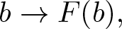 $b \to F(b),$
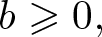 $b\geqslant0,$ but also of semiflow
 $\mathcal F^t \phi$ [Reference Smith31], see Section 2. As a consequence, the renewal equation
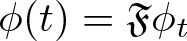 $\phi(t)=\frak F\phi_t$ and the one-dimensional system
 $b_{n+1}= {\frak F} b_n, \ b_n \in \mathbb R_+$, have identical dynamical structures. If
 $g$ is strictly decreasing, then the statement of Theorem 4 can be simplified: indeed, the inequalities
 $R(0) \gt 1$ and
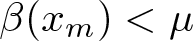 $\beta(x_m) \lt \mu$ guarantee fulfilment of the first condition in (i), the inequalities
 $R(0) \gt 1$ and
 $\beta(x_m)\geqslant\mu$ assure the first condition in (ii), and the assumption
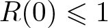 $R(0) \leqslant 1$ implies the first condition in (iii).
Also note that the type of local stability used in statement (i) of the above theorem is stronger than that one used in [Reference Barril, Calsina, Diekmann and Farkas4], where the closeness  $|b_t-\kappa|_\rho \lt \epsilon$,
 $t\geqslant0$, in the weighted integral norm
 $|\cdot|_\rho$ is obtained instead of the closeness in the uniform norm.
We conclude the introduction with a brief outline of the paper. In the next section, we examine the monotonicity property of the operator  ${\frak F}$. Theorems 2 and 4 are proved in Section 3, while Section 4 discusses possible directions for further study of equation (1.1). The proof of Proposition 1 is given in the Appendix.
2. Monotonicity of the operator
${\frak F}$

Theorem 5 Suppose that  $\beta$ is a non-decreasing continuous function of polynomial growth and
 $g:\mathbb{R}_+ \to \mathbb{R}_+$ is continuous and bounded. Then the operator
 ${\frak F}: L^1_\rho(\mathbb{R}_{-}, \mathbb{R}_+) \to \mathbb{R}_+$ defined by (1.6) is non-decreasing with respect to the natural order in
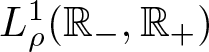 $L^1_\rho(\mathbb{R}_{-}, \mathbb{R}_+)$ for each
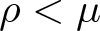 $\rho \lt \mu$.
Proof. First, we assume that 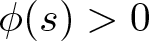 $\phi(s) \gt 0$ a.e. on
 $\mathbb{R}_-$. Set
 $h(s)=\phi(s)e^{\mu s}$ and
 $\theta = H(u)=\int_{-\infty}^uh(s)ds$, a straightforward computation shows that
 \begin{align*}
{\frak F}\phi&= \int_0^\infty \beta\left( x_m + \int_0^a g\left( e^{-\mu(\tau-a)} \int_a^\infty e^{-\mu s} \phi(-s) ds \right) d\tau \right) e^{-\mu a} \phi(-a) da \\
&= \int_{-\infty}^0 \beta\left( x_m + \int_u^0 g( e^{-\mu s} H(u) ) ds \right) h(u) du \\
&= \int_0^{H(0)} \beta\left( x_m + \int_{H^{-1}(\theta)}^0 g(e^{-\mu s} \theta) ds \right) d\theta.
\end{align*}
In general, the latter integral is an improper Riemann integral (can have a singularity at  $\theta =0$), and
 $H(u)$ is strictly increasing and positive on
 $\mathbb{R}$, with
 $H(-\infty)=0$.
If  $\phi_2(s)\geqslant\phi_1(s) \gt 0$, almost everywhere on
 $\mathbb{R}_-$, then clearly
 \begin{equation*}H_2(u)=\int_{-\infty}^uh_2(s)ds\geqslant H_1(u)=\int_{-\infty}^uh_1(s)ds,\quad u\leqslant0,\end{equation*}
so that
 \begin{equation*}
H_2^{-1}(\theta) \leqslant H_1^{-1}(\theta) \leqslant 0, \quad 0 \lt \theta \leqslant H_1(0).
\end{equation*}
 \begin{align*}
\mbox{Consequently}, \quad \mathfrak{F}\phi_2 &= \int_0^{H_2(0)} \beta\left( x_m + \int_{H_2^{-1}(\theta)}^0 g(e^{-\mu s} \theta ) ds \right) d\theta \\
&\geqslant \int_0^{H_1(0)} \beta\left( x_m + \int_{H_1^{-1}(\theta)}^0 g(e^{-\mu s} \theta) ds \right) d\theta =\mathfrak{F}\phi_1.
\end{align*}
Now, if  $\phi_2(s)\geqslant\phi_1(s)\geqslant0$, then the above argument shows that
 $\mathfrak F(\phi_2+\delta)\geqslant\mathfrak F(\phi_1+\delta)$ for each positive constant function
 $\delta$. Since
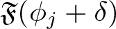 ${\frak F}(\phi_j +\delta)$ depends continuously on
 $\delta$, we obtain that
 $\mathfrak F\phi_2\geqslant\mathfrak F\phi_1$ by considering
 $\delta \to 0^+$. This completes the proof of Theorem 5.
Corollary 1. If  $\beta$ and
 $g$ satisfy all assumptions of Theorem 5 and
 $\beta(x_m+x) \gt 0$ for
 $x \gt 0$, then
 $F(b)$ is a strictly increasing function.
Proof. Indeed, 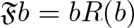 ${\frak F}b=bR(b)$ while for
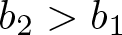 $b_2 \gt b_1$ we have
 $H_2(0) = b_2/\mu \gt H_1(0) = b_1/\mu$. See also Figure 1 for a graphical illustration.






3. Uniform ultimate boundedness and uniform persistence of solutions. Proofs of Theorems 3 and 5
Theorem 6 Assume that  $\beta(x+x_m)\leqslant \beta(x_m)+cx$ for some
 $c \gt 0$ and for all
 $x\geqslant0$,
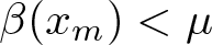 $\beta(x_m) \lt \mu$, that
 $g$ is a non-negative continuous function with
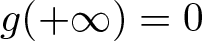 $g(+\infty)=0$. Let
 $b(t)$ denote the continuous solution to the initial value problem
 $b_0=\phi \in L^1_\rho(\mathbb{R}_{-}, \mathbb{R}_+)$ for (1.1). Then there are constants
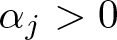 $\alpha_j \gt 0$ depending only on
 $\beta, g, \mu$, such that
 \begin{equation*}\limsup_{t\rightarrow+\infty}b(t)\leqslant\alpha_1\quad\text{and}\quad0\leqslant b(t)\leqslant\alpha_2\vert\phi\vert_\rho+\alpha_3,\quad t\geqslant0.\end{equation*}
Proof. Set  $H_t(a)=\int_{-\infty}^{a}e^{\mu s}b(t+s)ds$ and
 $h_t(a)=\frac{d}{da}H_t(a)=e^{\mu a}b(t+a)$. Then
 \begin{align*}
b(t) &= \int_{-\infty}^{0} \beta\left( x_m + \int_0^{-a} g\left( e^{-\mu(\tau + a)} \int_{-a}^\infty e^{-\mu s} b(t-s) ds \right) d\tau \right) e^{\mu a} b(t+a) da \\
&= \int_{-\infty}^0 \beta\left( x_m + \int_a^0 g\left( e^{-\mu \tau} \int_{-\infty}^a e^{\mu s} b(t+s) ds \right) d\tau \right) e^{\mu a} b(t+a) da \\
&= \int_{-\infty}^0 \beta\left( x_m + \int_a^0 g(e^{-\mu \tau} H_t(a)) d\tau \right) h_t(a) da \\
&\leqslant \int_{-\infty}^0 \left[ \beta(x_m) + c\int_a^0 g( e^{-\mu \tau} H_t(a) ) d\tau \right] h_t(a) da\\
&= \beta(x_m) \int_{-\infty}^0 h_t(a) da + c\int_{-\infty}^0 \int_a^0 g( e^{-\mu \tau} H_t(a) ) h_t(a) d\tau da =: J_1 + J_2.
\end{align*}
Next, observe that
 \begin{equation*}
J_1 = \beta(x_m) e^{-\mu t} \int_{-\infty}^t e^{\mu a} b(a) da = \beta(x_m)e^{-\mu t} |\phi|_\mu + \beta(x_m) e^{-\mu t} \int_0^t e^{\mu a} b(a)da.
\end{equation*}
Then, setting  $G(x) = \int_0^x g(t)\,dt$, we change the order of integration in
 $J_2$:
 \begin{align*}
J_2 &= c \int_{-\infty}^0 \int_{-\infty}^\tau g( e^{-\mu \tau} H_t(a) ) h_t(a) da d\tau \\
&= c\int_{-\infty}^0 e^{\mu \tau} \int_{-\infty}^\tau \frac{d}{da} [G(e^{-\mu \tau} H_t(a))] da d\tau
= c\int_{-\infty}^0 e^{\mu \tau} G( e^{-\mu \tau} H_t(\tau) ) d\tau,
\end{align*}
where we have used the fact that  $\lim_{a\to -\infty} G(e^{-\mu \tau} H_t(a) ) = G(0) = 0$. Moreover, as
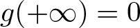 $g(+\infty)=0$, it follows that
 $G(x)/x \to 0$ as
 $x\to +\infty$. This implies that for each
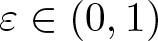 $\varepsilon\in (0,1)$ there exists a constant
 $C_\varepsilon$ such that
 $ G(x) \leqslant C_\varepsilon + \varepsilon x $ for all
 $x\geqslant0$. Thus
 \begin{align*}
J_2 &\leqslant c\int_{-\infty}^0 e^{\mu \tau} [C_\varepsilon + \varepsilon e^{-\mu \tau} H_t(\tau)] d\tau \\
&=\frac{cC_\varepsilon}{\mu} + \varepsilon c \int_{-\infty}^0 \int_{-\infty}^\tau e^{\mu s} b(t+s) ds d\tau
= \frac{c C_\varepsilon}{\mu} + \varepsilon c e^{-\mu t} \int_{-\infty}^0 \int_{-\infty}^{t+\tau} e^{\mu s} b(s) ds d\tau.
\end{align*}
Changing the order of integration once more, we obtain
 \begin{align*}
\int_{-\infty}^0 \int_{-\infty}^{t+\tau} e^{\mu s} b(s) ds d\tau &= \int_{-\infty}^t \int_{s-t}^0 e^{\mu s} b(s) d\tau ds \\
= \int_{-\infty}^t (t-s) e^{\mu s} b(s) ds
&= t |\phi|_\mu - \int_{-\infty}^0 s e^{\mu s} \phi(s) ds + \int_0^t (t-s) e^{\mu s} b(s) ds.
\end{align*}
Then, setting  $B(t) = e^{\mu t} b(t)$, we can combine all previous estimates to obtain
 \begin{equation*}
B(t) \leqslant \beta(x_m) |\phi|_\mu + \varepsilon c |\phi|_\mu t + \frac{c C_\varepsilon}{\mu}e^{\mu t} + \int_0^t [\beta(x_m) + \varepsilon c (t-a) ] B(a) da.
\end{equation*}
Iterating this inequality, where the right-hand side defines a Volterra-type operator, we find that 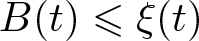 $B(t) \leqslant \xi(t)$, where
 $\xi(t)$ is a positive solution to the integral equation
 \begin{equation*}\xi(t)=\beta(x_m)\vert\phi\vert_\mu+c\varepsilon\vert\phi\vert_\mu t+\frac{cC_\varepsilon}\mu e^{\mu t}+\int_0^t\lbrack\beta(x_m)+c\varepsilon(t-a)\rbrack\xi(a)da,\quad t\geqslant0,\end{equation*}
see [Reference Beesack7, Theorem 5] for a comparison result for Volterra inequalities.
Clearly,  $\xi(t)$ also solves the initial value problem
 \begin{equation*}
\begin{cases} \xi''(t) = \mu c C_\varepsilon e^{\mu t} + \beta(x_m)\xi'(t) + \varepsilon c\xi(t) \\
\xi(0)=\beta(x_m) |\phi|_\mu + cC_\varepsilon \mu^{-1},~ \xi'(0)=\varepsilon c|\phi|_\mu + c C_\varepsilon + \beta(x_m)(\beta(x_m) |\phi|_\mu+cC_\varepsilon \mu^{-1}).
\end{cases}
\end{equation*}
Solving this problem, we obtain that
 \begin{equation*}
\xi(t) = \alpha_1 e^{\mu t} + a_1 e^{\lambda_+ t} + a_2 e^{\lambda_{-}t},
\end{equation*}
 \begin{equation*}\mbox{where }\quad \alpha_1 = \frac{\mu c C_\varepsilon}{\mu^2 - \mu \beta(x_m) - \varepsilon c}, \quad
\lambda_\pm = \frac{\beta(x_m) \pm \sqrt{\beta^2(x_m) + 4\varepsilon c}}{2},
\end{equation*}
and 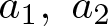 $a_1,~a_2$ are determined from the linear system
 \begin{equation*}
\begin{cases}
a_1 + a_2 &=\beta(x_m) |\phi|_\mu + cC_\varepsilon \mu^{-1}- \alpha_1,\\
\lambda_+ a_1 + \lambda_-a_2 &=-\alpha_1\mu +\varepsilon c|\phi|_\mu + c C_\varepsilon + \beta(x_m)(\beta(x_m) |\phi|_\mu +cC_\varepsilon \mu^{-1}).
\end{cases}
\end{equation*}
Since 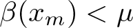 $\beta(x_m) \lt \mu$, we can take
 $\varepsilon \gt 0$ small enough to have
 $\lambda_{-} \lt \lambda_+ \lt \mu$. Thus, we conclude that
 \begin{equation*}b(t)\leqslant\alpha_1+a_1e^{(\lambda_+-\mu)t}+a_2e^{(\lambda_--\mu)t}\leqslant\alpha_1+\vert a_1\vert+\vert a_2\vert\leqslant\alpha_2\vert\phi\vert_\rho+\alpha_3,\quad t\geqslant0,\end{equation*}
 \begin{equation*}
\limsup_{t \to +\infty} b(t) \leqslant \alpha_1= \frac{\mu c C_\varepsilon}{\mu^2 - \mu \beta(x_m) - \varepsilon c},
\end{equation*}
with some  $\alpha_j$ independent of the initial data
 $\phi$.
Corollary 3. Suppose that  $\beta(x)$ is a globally Lipschitzian function with the Lipschitz constant
 $L$ (so that
 $\beta(x_m+x)\leqslant \beta_1(x):=\beta(x_m)+Lx$ for all
 $x\geqslant0$), that
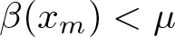 $\beta(x_m) \lt \mu$ and that
 $g$ is a non-negative continuous function with
 $g(+\infty)=0$. Then there are constants
 $\alpha_4, \alpha_5 \gt 0$ depending only on
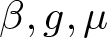 $\beta, g, \mu$ and such that the continuous solution
 $b(t)$ of the initial value problem
 $b_0=\phi \in L^1_\rho(\mathbb{R}_{-}, \mathbb{R}_+)$ for equation (1.1) is differentiable on
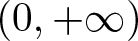 $(0,+\infty)$ and has a uniformly bounded derivative:
 \begin{equation}
|b'(t)| \leqslant \alpha_4|\phi|_\rho + \alpha_5, \quad t \gt 0.
\end{equation}
Proof. Note that
 \begin{align*}
b(t) &= \int_{-\infty}^t \beta\left( x_m + \int_a^t g\left( e^{-\mu \tau} \int_{-\infty}^a e^{\mu s} b(s) ds \right) d\tau \right) e^{-\mu(t-a)} b(a) da.
\end{align*}
By differentiating the last equality, we obtain
 \begin{align}b'(t)&= \beta(x_m)b(t) - \mu b(t) \nonumber \\
& + e^{-\mu t}\int_{-\infty}^t \frac{d}{dt} \left[ \beta\left( x_m + \int_a^t g\left( e^{-\mu \tau} \int_{-\infty}^a e^{\mu s} b(s) ds \right) d\tau \right) e^{\mu a} b(a) \right] da \nonumber \\
&= (\beta(x_m) - \mu) b(t) + \nonumber \\
e^{-\mu t}\int_{-\infty}^t & \beta'\left( x_m + \int_a^t g\left( e^{-\mu \tau} \int_{-\infty}^a e^{\mu s} b(s) ds \right) d\tau \right) g\left( e^{-\mu t} \int_{-\infty}^a e^{\mu s} b(s) ds \right) e^{\mu a} b(a) da.\end{align}
Thus, using the estimates  $|\beta'(x_m + x)|\leqslant L$ a.e. on
 $\mathbb{R}_+$, and
 $0 \leqslant b(t) \leqslant \alpha_2|\phi|_\rho + \alpha_3$,
 $t\geqslant0$, we find that
 \begin{align*}
|b'(t)| &\leqslant (\mu-\beta(x_m))(\alpha_2|\phi|_\rho + \alpha_3) + L \max_{x\geqslant 0} g(x) e^{-\mu t} \left[ |\phi|_\rho + \int_0^t e^{\mu a} b(a) da \right] \\
&\leqslant (\mu-\beta(x_m))(\alpha_2|\phi|_\rho + \alpha_3) + L \max_{x\geqslant 0} g(x) \left[ |\phi|_\rho + \frac{(\alpha_2|\phi|_\rho + \alpha_3)}{\mu} \right],
\end{align*}
and the estimate (3.1) follows.
Now, consider the operator  ${\frak F_1}$ defined by (1.6) where
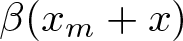 $\beta(x_m+x)$ is replaced with
 $\beta_1(x)=\beta(x_m)+Lx\geqslant\beta(x+x_m),x\geqslant0$ (cf. Corollary 3) and
 $g(+\infty)=0$. Clearly,
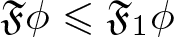 ${\frak F}\phi \leqslant {\frak F_1}\phi$ for each
 $\phi \in L^1_\rho(\mathbb{R}_{-}, \mathbb{R}_+)$. By Theorem 5, the functional
 ${\frak F_1}$ is monotone on
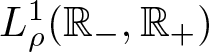 $L^1_\rho(\mathbb{R}_{-}, \mathbb{R}_+)$ and the monotone scalar function
 $F_1(c)= {\frak F_1}c$ (here
 $c$ is considered as a constant element of
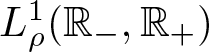 $L^1_\rho(\mathbb{R}_{-}, \mathbb{R}_+)$) has the representation
 $F_1(c)= cR_1(c)$ where
 \begin{equation*}
R_1(c):=\int_0^\infty \left(\beta(x_m) + L\int_0^a g\left( \frac{e^{-\mu\tau}}{\mu}c\right) d\tau \right) e^{-\mu a}da.\end{equation*}
We have that  $\textstyle R_1(0)\geqslant R(0) \gt 1,\;R_1(+\infty)=R(+\infty)=\beta(x_m)/\mu \lt 1,$ so that the set of positive solutions of the equation
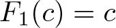 $F_1(c)=c$ (equivalently, of the equation
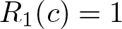 $R_1(c)=1$) is nonempty and compact. Let
 $\theta_2$ denote its maximal element (i.e., its supremum). Then
 $F_1(\theta_2)=\theta_2$ and
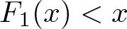 $F_1(x) \lt x$ for
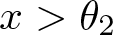 $x \gt \theta_2$.
Corollary 4. Assume all conditions of Corollary 3. If 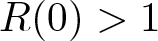 $R(0) \gt 1$, then each continuous non-zero bounded function
 $b(t)$ satisfying equation (1.1) for all
 $t \in \mathbb{R}$ has
 $\theta_2$ as an upper bound:
 $
0\leqslant b(t) \leqslant \theta_2, \quad t \in \mathbb{R}.
$
Proof. Without loss of generality, after using an appropriate translation or applying a limiting argument, we can assume that  $b(0)= \max_{s \in \mathbb{R}}b(s)$. But then
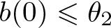 $b(0) \leqslant \theta_2$ as a consequence of the chain of inequalities
 $b(0)= {\frak F}b_0 \leqslant {\frak F_1}b_0 \leqslant {\frak F_1}b(0)= F_1(b(0))$ and the above mentioned property
 $F_1(x) \lt x$ for
 $x \gt \theta_2$.
Corollary 5. Assume all conditions of Corollary 3 and that  $g(x) \gt 0$ for all
 $x\geqslant0$,
 $\beta(x) \gt 0$ a.e. on
 $[x_0,+\infty)$ for some
 $x_0\geqslant x_m$. If
 $R(0) \gt 1$, then the semiflow
 $\mathcal F^t \phi$ is uniformly persistent: i.e., there exists
 $\theta_1 \gt 0$ such that
 $\liminf_{t\rightarrow\infty}b(t)\geqslant\theta_1$ for each non-zero solution
 $b(t)$.
Proof. Let  $C_b$ denote the space of all continuous bounded functions
 $c:\mathbb{R}_+\to \mathbb{R}_+$ endowed with the sup-norm. The functional
 ${\mathcal R}: C_b \to \mathbb{R}_+$ defined by
 \begin{equation*}
{\mathcal R}(c)=\int_0^\infty \beta\left( x_m + \int_0^a g\left( \frac{e^{-\mu\tau}}{\mu} c(a) \right) d\tau \right) e^{-\mu a}da
\end{equation*}
is clearly continuous at  $c=0$ and therefore there exists some
 $\delta \gt 0$ such that
 \begin{equation}\sigma:=\inf\left\{\mathcal R(c):c\in C_b,\;c(a)\in\lbrack0,\delta\rbrack,a\geqslant0\right\} \gt 1.\end{equation}
We start by proving the impossibility of the convergence  $\lim_{t\to \infty} b(t)=0$ for an eventually positive solution
 $b(t)$. Due to Proposition 1(d), without loss of generality, we can assume that
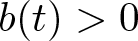 $b(t) \gt 0$ for all
 $t\geqslant0$. If
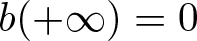 $b(+\infty)=0$, there exists an increasing sequence of numbers
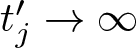 $t'_j\to \infty$, such that
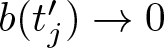 $b(t'_j)\to 0$ and
 $0 \lt b(t'_j)\leqslant b(t)$ for all
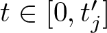 $t \in [0,t'_j]$. Then we get from (1.1) that
 \begin{align*}
b(t_j')&\geqslant \int_0^{t_j'} \beta\left( x_m + \int_0^a g\left( e^{-\mu(\tau - a)} \int_a^\infty e^{-\mu s} b(t_j' - s) ds \right) d\tau \right) e^{-\mu a} b(t_j'-a) da \\
&\geqslant \int_0^{t_j'} \beta\left( x_m + \int_0^ag\left( e^{-\mu(\tau - a)} \int_a^\infty e^{-\mu s} b(t_j' - s) ds \right) d\tau \right) e^{-\mu a} b(t_j') da.
\end{align*}
Consequently,
 \begin{equation}1\geqslant\int_0^{t'_j}\beta\left(x_m+\int_0^ag\left(e^{-\mu(\tau-a)}\int_a^\infty e^{-\mu s}b(t_j'-s)ds\right)d\tau\right)e^{-\mu a}da.\end{equation}
Taking the limit in the latter inequality as 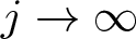 $j \to \infty$, we obtain that
 \begin{equation*}1\geqslant\int_0^\infty\beta(x_m+ag(0))e^{-\mu a}da=R(0) \gt 1,\end{equation*}
a contradiction. Consequently,  $\limsup_{t\to \infty} b(t) \gt 0$ for each non-zero solution
 $b(t)$.
Let us assume now that the semiflow  $\mathcal F^t \phi$ is not uniformly persistent, i.e., for each
 $n$ there exists a non-zero solution
 $b_n(t)$ such that
 $\liminf_{t\to \infty} b_n(t) \lt 1/n$. Using, if necessary, appropriately shifted solutions
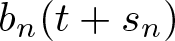 $b_n(t+s_n)$ with
 $s_n\geqslant0$ and invoking the ultimate uniform boundedness result of Theorem 6, without loss of generality, we can assume that
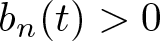 $b_n(t) \gt 0$ for all
 $t\geqslant0$ and that the sequence of the initial segments
 $\phi_n(s)=b_n(s), \ s \lt 0$, is bounded in
 $L^1_\rho(\mathbb{R}_{-}, \mathbb{R}_+)$. In view of (3.1), this implies the uniform boundedness of the sequence
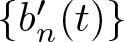 $\{b'_n(t)\}$ on
 $\mathbb{R}_+$.
With  $\delta \gt 0$ and
 $\sigma \gt 1$ chosen so as to satisfy (3.3), we consider the following two cases:
Case 1. For some 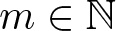 $m \in \mathbb{N}$ it holds that
 \begin{equation}
0\leqslant \zeta_1 =:\liminf_{t\to \infty} b_m(t) \leqslant \limsup_{t\to \infty} b_m(t):=\zeta_2\leqslant \delta, \quad \zeta_2 \gt 0.
\end{equation}
If 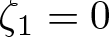 $ \zeta_1=0$ then there exists a monotone sequence
 $s_k \to +\infty$ such that
 $\lim_{k\to \infty} b_m(s_k)=0$ and
 $0 \lt b_m(s_k)\leqslant b_m(t)$ for all
 $t \in [0,s_k]$. Since Equation (1.1) is translation invariant, the functions
 $b_{m,j}(t):=b_m(t+s_j)$ are also solutions of it. By invoking the Arzelá–Ascoli theorem and using Theorem 6 and Corollary 3, we may conclude that some subsequence
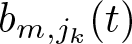 $b_{m,j_k}(t)$ is converging, uniformly on compact subsets of
 $\mathbb{R}$, to a continuous function
 $b_*(t)$ such that
 $b_*(t)\leqslant \zeta_2\leqslant \delta$,
 $t \in \mathbb{R}$. Arguing as above of the formula (3.4), we also obtain
 \begin{equation*}1\geqslant\int_0^{s_{j_k}}\beta\left(x_m+\int_0^ag\left(e^{-\mu(\tau-a)}\int_a^\infty e^{-\mu s}b_m(s_{j_k}-s)ds\right)d\tau\right)e^{-\mu a}da.\end{equation*}
After passing to the limit in this inequality as  $k \to \infty$, we obtain the contradiction
 \begin{equation*}1\geqslant\int_0^\infty\beta\left(x_m+\int_0^ag\left(\frac{e^{-\mu\tau}}\mu e^{\mu a}\mu\int_a^\infty e^{-\mu s}b_\ast(-s)ds\right)d\tau\right)e^{-\mu a}da \gt 1,\end{equation*}
which follows from the definition of  $\delta$ in (3.3) together with the estimate
 \begin{equation}0\leqslant c(a)=e^{\mu a}\mu\int_a^\infty e^{-\mu s}b_\ast(-s)\,ds\leqslant\delta,\quad a\geqslant0.\end{equation}
If  $ \zeta_1 \gt 0$, we can modify the previous argumentation as follows. Take
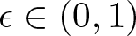 $\epsilon \in (0, 1)$ small enough to satisfy
 $(1-\epsilon)\sigma \gt 1$. We can also assume that
 $b_m(t)\geqslant\zeta_1(1-\epsilon)$ for all
 $t\geqslant0$. Then there exists a monotone sequence
 $s_k \to +\infty$ such that
 $\lim_{k\to \infty} b_m(s_k)=\zeta_1$. Choose a continuous function
 $b_*(t)$ as above. Then
 \begin{align*}
&b_m(s_k)/(\zeta_1(1-\epsilon)) \\
&\quad \geqslant \int_0^{s_k} \beta\left( x_m + \int_0^a g\left( e^{-\mu(\tau - a)} \int_a^\infty e^{-\mu s} b_m(s_k-s) ds \right) d\tau \right) e^{-\mu a} da
\end{align*}
After taking the limit in this inequality as 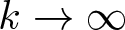 $k \to \infty$, we get the following contradiction
 \begin{equation*}1/(1-\epsilon)\geqslant\int_0^\infty\beta\left(x_m+\int_0^ag\left(e^{-\mu(\tau-a)}\int_a^\infty e^{-\mu s}b_\ast(-s)ds\right)d\tau\right)e^{-\mu a}da\geqslant\sigma,\end{equation*}
in view of (3.6). Thus, the situation presented in formula (3.5) cannot happen.
Case 2. For each  $n \in \mathbb{N}, \ n \gt 1/\delta$, it holds that
 \begin{equation*}
0\leqslant \zeta_n =:\liminf_{t\to \infty} b_n(t) \lt 1/n \lt \delta \lt \limsup_{t\to \infty} b_n(t).
\end{equation*}
Then for each fixed  $n \gt 1/\delta$, there are increasing sequences of positive numbers
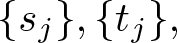 $\{s_j\}, \{t_j\},$
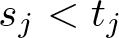 $s_j \lt t_j$ such that
 $s_j, t_j\to \infty$,
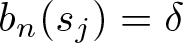 $b_n(s_j)=\delta$,
 $b_n(t_j) = 1/n$, and
 $1/n\leqslant b_n(t) \leqslant \delta$ for all
 $t \in [s_j,t_j]$. Choose some converging subsequence
 $t_{j_k}-s_{j_k} \to \tau_n \in [0,+\infty]$. Since equation (1.1) is translation invariant, the functions
 $b_{n,j}(t)=b_n(t+s_j)$ are also solutions of it. By invoking the Arzelá–Ascoli theorem and using Theorem 6 and Corollary 3, we may conclude that some subsequence
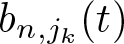 $b_{n, j_k}(t)$ is converging, uniformly on compact subsets of
 $\mathbb{R}$, to a continuous bounded function
 $d_n(t)$ such that
 $d_n(0)= \delta= \max_{s \in [0, \tau_n]}d_n(s)$. Since
 $\limsup_{t\to \infty} d_n(t) \gt 0$, the option
 $\tau_n= +\infty$ is not possible in view of the analysis done in Case 1. Therefore,
 $\tau_n$ is a finite positive number and
 $d_n(\tau_n)=1/n$. Clearly, the sequences
 $d_n(t)$ and
 $d'_n(t)$ are uniformly bounded on
 $\mathbb{R}$. Therefore, once more applying the Arzelá-Ascoli theorem, we find some subsequence
 $i_k$ and an extended positive number
 $\tau_\star \in [0, +\infty]$ such that
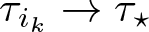 $\tau_{i_k} \to \tau_\star$ and
 $d_{i_k}(t)$ is converging, uniformly on compact subsets of
 $\mathbb{R}$, to a continuous bounded function
 $d_\star(t)$ such that
 $d_\star(0)= \delta= \max_{s \in [0,\tau_\star]}b(s)$ and
 $\limsup_{t\to \infty} d_\star(t) \gt 0$. Once again, the possibility
 $\tau_\star = +\infty$ is excluded by the analysis in Case 1. Hence,
 $\tau_\star$ is a finite positive number with
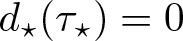 $d_\star(\tau_\star) = 0$. Yet, because
 $d_\star(t)$ satisfies (1.1) for all
 $t \in \mathbb{R}$ and
 $d_\star(0) = \delta \gt 0$, we must have
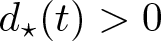 $d_\star(t) \gt 0$ for all
 $t \in \mathbb{R}$. This contradiction concludes the proof of Corollary 5.
Proof of Theorem 2
Let  $\mathcal B$ comprises all continuous functions
 $\phi: (-\infty,0] \to [0,+\infty)$ such that
 $0.5\theta_1 \leqslant \phi(t) \leqslant 2\theta_2,\ t \leqslant 0,$ with
 $\theta_j$ defined in Corollaries 4 and 5. Then
 $\mathcal B$ is bounded in
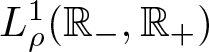 $L^1_\rho(\mathbb{R}_{-}, \mathbb{R}_+)$ by
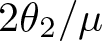 $2\theta_2/\mu$. Next, consider the subset
 $\mathcal D$ of
 $\mathcal B$ consisting from all Lipschitzian functions with the Lipschitz constant which is less or equal to
 $\theta_3:= 2\alpha_4\theta_2/\mu + \alpha_5$ with
 $\alpha_4, \alpha_5$ being defined in Corollary 3. Clearly,
 $\mathcal D$ is a compact subset of
 $L^1_\rho(\mathbb{R}_{-}, \mathbb{R}_+)$ attracting every positive solution due to Corollaries 3, 4, and 5. This fact implies the existence of the compact attractor
 $\mathcal A$ of points (e.g., see [Reference Smith and Thieme32, Theorem 2.17(c)]) possessing properties mentioned in the statement of Theorem 2.
Proof of Theorem 4
(i) Set  $\theta_1\leqslant m= \inf_{\phi \in \mathcal A}\phi(0); \ M= \sup_{\phi \in \mathcal A}\phi(0) $. Clearly,
 $\theta_1\leqslant m \leqslant M \leqslant \theta_2$ and, by Corollary 2, we find that
 $[m,M] \subseteq [F(m),F(M)]$. In view of the uniqueness of the positive equilibrium
 $b_*$ and the monotonicity of
 $F(x)$ having
 $F'(0)=R(0) \gt 1$ with
 $ \lim_{b \to +\infty}F(b)/b = \beta(x_m)/\mu \lt 1$, this can happen if and only if
 $m=M=b_*$. Thus
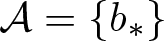 $\mathcal A= \{b_*\}$. Let us now suppose that the equilibrium
 $b_*$ is not stable as indicated in the statement of the theorem. Then there is
 $\epsilon \in (0,b_*/2)$ and a sequence
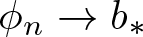 $\phi_n \to b_*$ such that corresponding solutions
 $b_n(t)$ satisfy the estimate
 $
\sup_{t \leqslant 0}|b_n(t)-b_*| \gt \epsilon, $
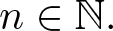 $n \in \mathbb{N}.
$ Since
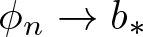 $\phi_n \to b_*$, the sequences
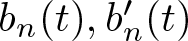 $b_n(t), b'_n(t)$ are uniformly bounded on
 $\mathbb{R}_+$ and
 $b_n(t)$ converges uniformly to
 $b_*$ on the intervals
 $[0,j]$,
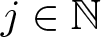 $j \in \mathbb{N}$. Since
 $b_n(+\infty) = b_*$, there exists a sequence
 $s_n$ of positive numbers such that
 \begin{equation}
\max_{t \in [0,s_n]}|b_n(t)-b_*| = |b_n(s_n)-b_*|= \epsilon \in (0,b_*/2).
\end{equation}
It is clear that  $s_n \to \infty$. But then, considering a sequence of shifted solutions
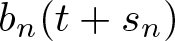 $b_n(t+s_n)$ and using a limiting argument, we establish the existence of a bounded continuous function
 $b_*(t)$ satisfying equation (1.1) for all
 $t \in \mathbb{R}$ and such that
 \begin{equation*}\sup_{t\in\mathbb{R}}\vert b_\ast(t)-b_\ast\vert\geqslant\vert b_\ast(0)-b_\ast\vert=\max_{t\leqslant0}\vert b_\ast(t)-b_\ast\vert=\epsilon \lt b_\ast/2 .\end{equation*}
This means that either  $M_*:=\sup_{t\in\mathbb R} b_*(t)$ or
 $m_*:=\inf_{t\in\mathbb R} b_*(t)$ differs from
 $b_*$. Moreover, since
 $b_*(+\infty)=b_*$ and
 $b_*(t)\geqslant b_*/2$ for all
 $t\leqslant 0$, we necessarily have
 $m_* \gt 0$. Indeed, if
 $m_*=0$, then there would exist
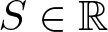 $S\in \mathbb R$ such that
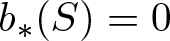 $b_*(S)=0$ while
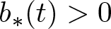 $b_*(t) \gt 0$ for all
 $t \lt S$, which is impossible in view of (1.1) and assumption (M*). Then the inclusion
 $[m_*,M_*] \subseteq [F(m_*),F(M_*)]$ implies
 $m_*=M_*=b_*$, which yields a contradiction. This contradiction proves the stability of
 $b_*$.
Next, choose  $\delta \gt 0$ small enough to have
 $\theta_1\leqslant b(t,\phi)\leqslant\theta_2,\;t\geqslant
0$, for each initial function
 $\phi$ satisfying
 $|\phi-b_*|_\rho \leqslant \delta$. We claim that
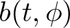 $b(t, \phi)$ converges to
 $b_*$ uniformly on the ball
 $B_\delta= \{\phi: |\phi-b_*|_\rho \leqslant \delta\}$. Indeed, otherwise there is
 $\gamma \gt 0$ and sequences
 $\phi_n \in B_\delta$ and
 $s_n \to + \infty$ such that
 $|b(s_n,\phi_n)-b_*|=\gamma$. Then, arguing as in the previous paragraph below (3.7), we obtain a contradiction. Hence,
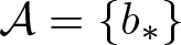 $\mathcal A= \{b_*\}$ attracts its neighbourhood
 $B_\delta$ and therefore it also attracts neighbourhoods of compact sets in
 $L^1_\rho(\mathbb{R}_{-}, \mathbb{R}_+)\setminus \{0\}$, e.g., see [Reference Smith and Thieme32, Corollary 2.32].
(ii) Assume that 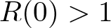 $R(0) \gt 1$ and
 $F(x) \not=x$ for
 $x \gt 0$. Then necessarily
 $\lim_{b\rightarrow+\infty}R(b)=\beta(x_m)/\mu\geqslant1$ so that
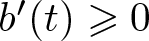 $b'(t)\geqslant 0$ in view of (3.2). Thus, we conclude that
 $b(t)$ is a non-decreasing function. If
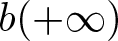 $b(+\infty)$ were finite, the constant function
 $b(t)=b(+\infty)$ should be an equilibrium for Equation (1.1) and therefore it should satisfy the equation
 $R(b(+\infty)) =1$, which is not possible if
 $b(\cdot)\not\equiv 0$ on
 $\mathbb{R}_+$.
(iii) We claim that 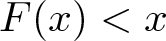 $F(x) \lt x$,
 $x \gt 0$, and (M*) imply that
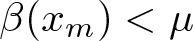 $\beta(x_m) \lt \mu$. Indeed, since
 $\beta(x)$ is increasing, we have that
 $R(b)\geqslant \beta(x_m)/\mu$ for all
 $b\geqslant 0$. Then
 $F'(0)=R(0) \leqslant 1$ assures that
 $\beta(x_m) \leqslant \mu$. Now, if
 $\beta(x_m) = \mu$ then
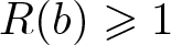 $R(b)\geqslant 1$,
 $b\geqslant 0$, so that
 $F(b)=bR(b)\geqslant b$ for all
 $b\geqslant0$, a contradiction. Therefore, in view of Theorem 6, each solution is eventually bounded while
 $[m,M] \subseteq [F(m),F(M)]$ and
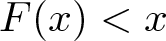 $F(x) \lt x$,
 $x \gt 0$ imply that
 $m=M=0$. Observe that
 $b_*=0$ when
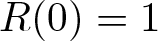 $R(0)=1$.
4. Discussion and open problems
Our study leads to a broader framework for scalar renewal equations of the form
 \begin{equation}
\phi(t) = \mathfrak{F} \phi_t, \quad \mbox{where} \ {\frak F}\phi:=\int_0^\infty B_\phi(a) e^{-\mu a} \phi(-a)da,
\end{equation}
considered in the phase space  $L^1_\rho(\mathbb{R}_{-})$,
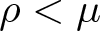 $\rho \lt \mu$, with the property that the associated real-valued function
 $
F(b) := \mathfrak{F} b, \ b \in \mathbb{R},
$ is strictly increasing. Note that
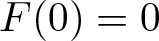 $F(0) = 0$ and therefore
 $F(b) \gt 0$ for
 $b \gt 0$. In (4.1), we naturally assume that
 $B_\phi(a)$ depends continuously on
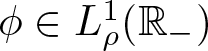 $\phi \in L^1_\rho(\mathbb{R}_{-})$ and on
 $a\geqslant0$. This formulation encompasses both (1.1) and (1.4). Consider the simplest scenario where
 $F$ has a unique equilibrium
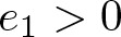 $e_1 \gt 0$ with
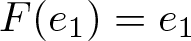 $F(e_1) = e_1$ and
 $F'(0) \gt 1 \gt F'(e_1)$. In this case,
 $e_1$ is a globally asymptotically stable fixed point of
 $F : (0,\infty) \to (0,\infty)$. An open problem is to determine the conditions on
 $B_\phi(a)$ under which the steady state
 $\phi(t) \equiv e_1$ of (1.4) likewise attracts all nonzero solutions of (4.1).
In the case of equation (1.4), the answer to the above problem is straightforward. Indeed, the function  $
f(b) ={F(b)}/{\int_0^\infty \beta(a)\,da}
$ is strictly increasing. Consequently, the functional
 $
\mathfrak{F} \phi = \int_0^\infty \beta(a)\, f(\phi(-a))\, da
$ is also strictly increasing, and the global attractivity of
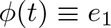 $\phi(t) \equiv e_1$ follows; see [Reference Herrera and Trofimchuk21] for details and further generalizations.
The situation for more complex renewal equations of type (1.1) is considerably more involved. In particular, taking in (1.1) the unimodal functions  $\beta(x) = \alpha x e^{-x}$ and
 $g(x) = p e^{-x}$ (this case is opposite to that studied in Theorem 4), we found in [Reference Herrera, Trofimchuk, Wood, Etheridge, de Gier and Joshi22] that
 $F(b)$ is strictly increasing for all choices of the parameters
 $\alpha$ and
 $p$. However, as shown in [Reference Hasik, Kopfová, Nábělková and Trofimchuk19, Example 2.4] for the specific parameter values
 $\alpha = 6$ and
 $p = 1$, such monotonicity of
 $F$ does not imply monotonicity—nor even the weaker property of quasi-monotonicity defined in [Reference Hasik, Kopfová, Nábělková and Trofimchuk19]—for the functional
 $\mathfrak{F}$. Nevertheless, for (1.1) with
 $\beta(x) = 6x e^{-x}$ and
 $g(x) = e^{-x}$, the unique positive equilibrium is globally asymptotically stable. The proof of this fact is nontrivial and requires verified numerics; see [Reference Hasik, Kopfová, Nábělková and Trofimchuk19, Example 3.3].
Furthermore, in [Reference Hasik, Kopfová, Nábělková and Trofimchuk19, Reference Herrera, Trofimchuk, Wood, Etheridge, de Gier and Joshi22] we provide additional numerical and analytical evidence shedding light on the possible structures of the global attractor  $\mathcal{A}$ when
 $F(b) = bR(b)$ is strictly increasing and has multiple fixed points. As shown in [Reference Herrera, Trofimchuk, Wood, Etheridge, de Gier and Joshi22], this situation may occur for the hump-shaped fertility function
 $\beta(x) = \alpha x e^{-x}$ and the strictly decreasing function
 $g(x) = p e^{-x}$. For instance,
 $R(b)$ may have a unimodal shape that produces three fixed points
 $e_1 = 0 \lt e_2 \lt e_3$ of
 $F$ for certain parameter values
 $\alpha, p$, even when
 $R(0) \lt 1$; this phenomenon corresponds to the Allee effect in the model. Then the general stability theorem from [Reference Diekmann and Gyllenberg13] (in view of the smoothness properties of the functional
 $\frak F$ proven in [Reference Barril, Calsina, Diekmann and Farkas4, Reference Barril, Calsina, Diekmann and Farkas5] and analysis of characteristic equations in [Reference Herrera, Trofimchuk, Wood, Etheridge, de Gier and Joshi22]) shows that the local stability properties of equilibria
 $e_j$ for the renewal equation
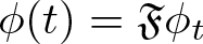 $\phi(t)=\frak F\phi_t$ and for one-dimensional system
 $b_{n+1}= F(b_n):= \frak F b_n, \ b_n \in \mathbb{R}$, coincide (at least, in non-degenerate equilibria
 $e_j$ when
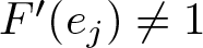 $F'(e_j)\not =1$). The described situation with one-dimensional map
 $F$ having positive monotone feedback at all equilibria suggests to look for an analogy with the theory developed in [Reference Krisztin and Walther23, Reference Krisztin, Walther and Wu24]. Particularly, in the mentioned case of three equilibria
 $e_1=0 \lt e_2 \lt e_3$, we can expect that the global attractor
 $\mathcal A$ has a form of a spindle (three-dimensional or degenerate one-dimensional) whose tip corresponds to the stable equilibria
 $e_1, e_3$, attracting all trajectories starting outside of a certain co-dimension 1 invariant manifold containing
 $e_2$. Therefore, we can expect that a typical solution
 $b(t)$ should satisfy either
 $b(+\infty)= e_1=0$ or
 $b(+\infty)= e_3 \gt 0$. Our numerical simulations in [Reference Herrera, Trofimchuk, Wood, Etheridge, de Gier and Joshi22], together with the additional considerations in [Reference Hasik, Kopfová, Nábělková and Trofimchuk19], support this heuristic conclusion and, perhaps surprisingly, suggest that a Hopf bifurcation at the unstable equilibrium
 $e_2$ is unlikely.
Acknowledgements
We are indebted to the Referee for the insightful and thorough reading of the manuscript, as well as for the valuable comments and detailed report, which have led to significant improvements in this revised version. The authors are deeply grateful to the late Pierre Magal and to Quentin Griette for stimulating discussions during the Winter School on Mathematical Modelling in Epidemiology and Medicine (2023, Valparaíso, Chile), particularly concerning the approaches developed in [Reference Herrera and Trofimchuk21, Reference Ma and Magal25], and for drawing our attention to the works [Reference Magal and Zhang27, Reference Smith30, Reference Webb33]. Pierre Magal’s insight, generosity, and enthusiasm were a lasting source of inspiration to us, and we are honoured to dedicate this work to his memory.
This research was supported by the projects FONDECYT 1231169 and AMSUD220002 (ANID, Chile). The first author was supported by ANID-Subdirección de Capital Humano/Doctorado Nacional/2024–21240616.
Appendix A. Appendix: Proof of Proposition 1
Proof of Proposition 1
Note that the condition of polynomial growth of  $\beta$ is sufficient to ensure that
 $r_\phi(t)$ is well defined for all
 $t\geqslant0$. Indeed, we have that
 \begin{align}r_\phi(t) &= \int_{-\infty}^0 \beta\left( x_m+ \int_a^t g\left( e^{-\mu \tau} \int_{-\infty}^a e^{\mu s}\phi(s)ds \right) d\tau \right) e^{-\mu(t-a)}\phi(a)da \nonumber \\
&= e^{-\mu t}\int_{-\infty}^0 \beta\left( x_m+ \int_a^t g\left( e^{-\mu \tau} \int_{-\infty}^a e^{\mu s}\phi(s)ds \right) d\tau \right) e^{(\mu-\rho)a}e^{\rho a}\phi(a)da,\end{align}
so that, for some 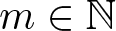 $m \in \mathbb{N}$,
 $r_\phi(t)= O(t^me^{-\mu t})$ at
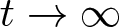 $t\to\infty$.
Part (a) Let 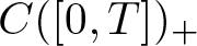 $C([0,T])_+$ be the space of nonnegative continuous functions on
 $[0,T]$, endowed with the uniform topology. Fix
 $T \gt 0$,
 $\phi\in L^1_\rho(\mathbb{R}_{-},\mathbb{R}_+)$ and define
 $\mathcal{A} : C([0,T])_+ \to C([0,T])_+$ by
 $\mathcal{A}b = \mathcal{V}_\phi b + r_\phi$. It is straightforward to check that
 $\mathcal{A}$ satisfies the conditions of the Schauder fixed-point theorem. Moreover, there exists norm
 $\|\cdot\|$ in
 $C([0,T])$ generating the topology of uniform convergence and
 $R_0=R_0(T) \gt 0$ for which
 $\mathcal{A} B_R \subseteq B_R$ for every
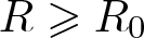 $R\geqslant R_0$, where
 $B_R\subseteq C([0,T])_+$ denotes the subset of functions with norm less or equal to
 $R$. Thus equation
 $b = \mathcal{V}_\phi b + r_\phi$ has at least one solution
 $b= b_T(\phi)$ in
 $B_R$ defined on the interval
 $[0,T]$.
Next, keeping  $\phi$ fixed, for each
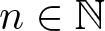 $n\in\mathbb N$ we consider the continuous solution
 $b_n(\phi)$ of (1.1), whose existence was established in the previous paragraph. Each solution
 $b_n(\phi)$ is defined on the finite interval
 $[0,n]$. For every fixed
 $N\in \mathbb{N}$, the sequence
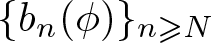 $\{b_n(\phi)\}_{n\geqslant N}$ is uniformly bounded and equicontinuous in
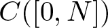 $C([0,N])$. In fact, by taking
 $\theta \gt 0$ large enough and considering the norm
 $\| b \|_\theta = \max_{t\in [0,N]} |e^{-\theta t} b(t)|$, we can prove that there is a positive number
 $\alpha$ such that
 $\Arrowvert b_n(\phi)\Arrowvert_\theta\leqslant\alpha\max_{t\geqslant0}r_\phi(t)$ for every
 $n\geqslant N$. This property of the family
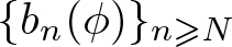 $\{b_n(\phi)\}_{n\geqslant N}$ assures its equicontinuity. Then the Arzelá–Ascoli theorem allows us to construct a continuous solution to (1.1) on
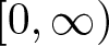 $[0,\infty)$ by means of a diagonal argument.
Part (b). Fix again 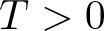 $T \gt 0$ and
 $\phi \in L^1_\rho(\mathbb{R}_{-},\mathbb{R}_+)$. Since the argument of
 $\beta$ in the expression for
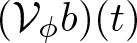 $(\mathcal{V}_\phi b)(t)$ is changing between
 $x_m$ and
 $x_m+T\sup_{s\geqslant0}g(s)$, without loss of generality, we may suppose that
 $\beta$ is a globally Lipschitzian function. If
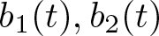 $b_1(t), b_2(t)$ solve equation (1.1) on
 $[0,T]$ with the same initial datum
 $b_2(s)=b_1(s)=\phi(s),s\leqslant 0$, then it follows from (a) and the proof of Corollary 3 that
 $\vert b_j(t)\vert+\vert b'_j(t)\vert\leqslant M,$
 $t \in [0,T]$, with some universal constant
 $M$. It can be also proved that
 \begin{equation}\vert b_2(t)-b_1(t)\vert\leqslant\int_0^tK(t,s)\vert b_2(s)-b_1(s)\vert ds,\quad t\in\lbrack0,T\rbrack,\end{equation}
with some non-negative function 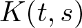 $K(t,s)$ (depending on
 $b_j(t)$) which is continuous on the closed triangle
 $\{(s,t):0\leqslant s\leqslant t\leqslant T\}$. Then an application of the Gronwall–Bellman type inequality (e.g., see [Reference Beesack7, Theorem 5]) shows that
 $b_1(t)\equiv b_2(t)$ on
 $[0,T]$.
To prove (A.2), we consider the cases  $\phi=0$ (with
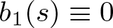 $b_1(s)\equiv 0$ and
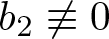 $b_2\not\equiv 0$) and
 $\phi\neq 0$ separately. The first case is trivial, and in the latter case, we avoid imposing the Lipschitz condition on
 $g$ by using the following estimates (where we set
 $B_j(a)= \int_{-\infty}^a e^{\mu s}b_j(s)ds$)
 \begin{equation*}
\left|\int_a^t g\left( e^{-\mu \tau} \int_{-\infty}^a e^{\mu s}b_2(s)ds \right) d\tau - \int_a^t g\left( e^{-\mu \tau} \int_{-\infty}^a e^{\mu s}b_1(s)ds \right) d\tau\right| =
\end{equation*}
 \begin{equation*}
\frac 1 \mu\left| \int_{e^{-\mu a}B_2(a)}^{e^{-\mu t}B_2(a)}(g(s)/s)ds- \int_{e^{-\mu a}B_1(a)}^{e^{-\mu t}B_1(a)}(g(s)/s)ds\right| =
\end{equation*}
 \begin{equation*}\frac1\mu\left|-\int_{e^{-\mu a}B_1(a)}^{e^{-\mu a}B_2(a)}(g(s)/s)ds+\int_{e^{-\mu t}B_1(a)}^{e^{-\mu t}B_2(a)}(g(s)/s)ds\right|\leqslant\end{equation*}
 \begin{equation*}\frac{2\sup_{s\geqslant0}g(s)}\mu\left|\ln\frac{B_2(a)}{B_1(a)}\right|\leqslant\frac{2\sup_{s\geqslant0}g(s)}\mu\left|\ln\left(1+\frac{\int_0^ae^{\mu s}\vert b_2(s)-b_1(s)\vert ds}{B_1(0)}\right)\right|\leqslant\end{equation*}
 \begin{equation*}\frac{2\sup_{s\geqslant0}g(s)}{\mu\vert\phi\vert_\mu}\int_0^te^{\mu s}\vert b_2(s)-b_1(s)\vert ds,\quad0\leqslant a\leqslant t.\end{equation*}
Part (c). To prove that the solution  $b_\phi$ depends continuously on
 $\phi \in L^1_\rho(\mathbb{R}_{-},\mathbb{R}_+)$, take an arbitrary initial function
 $\phi_0$ in this space and consider the sequence
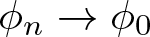 $\phi_n \to \phi_0$ together with the sequence of respective solutions
 $b_n(t)$ and
 $b_0(t)$ for Equation (1.1) on
 $[0,T]$. If the sequence
 $b_n(t)$ does not converge uniformly to
 $b_0(t)$, then it contains a subsequence
 $b_{n_j}(t)$ converging uniformly to some
 $b_*(t) \not= b_0(t)$, see proofs in (a), (b). Then, taking the limit as
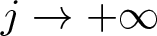 $j \to +\infty$ in the renewal equations (1.1) for
 $b_{n_j}(t)$, we obtain that the limiting function
 $b_*(t)$ also solves (1.1) with the initial data
 $\phi_0$. This, however, contradicts the uniqueness result established in (b).
Part (d). Consider Equation (1.1) in the Volterra’s form  $b(t) = (\mathcal{V}_\phi b)(t) + r_\phi(t)$. Since
 $({\mathcal V}_\phi b)(t)\geqslant0$ for
 $t\geqslant0$, it suffices to prove that
 $\phi\not=0$ implies
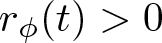 $r_\phi(t) \gt 0$ for all
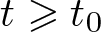 $t\geqslant t_0$ and some
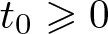 $t_0\geqslant0$. Let
 $A \lt 0$ be such that
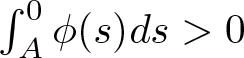 $\int_A^0\phi(s)ds \gt 0$. Then it follows from (A.1) that
 \begin{equation*}r_\phi(t)e^{\mu t}\geqslant\int_A^0\beta\left(x_m+\int_a^tg\left(e^{-\mu\tau}\int_{-\infty}^ae^{\mu s}\phi(s)ds\right)d\tau\right)e^{\mu a}\phi(a)da.\end{equation*}
Since for all 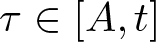 $\tau \in [A, t]$ and
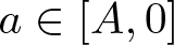 $a\in [A,0]$, it holds that
 \begin{equation*}0\leqslant e^{-\mu\tau}\int_{-\infty}^ae^{\mu s}\phi(s)ds\leqslant\Gamma:=e^{-\mu A}\vert\phi\vert_\mu,\end{equation*}
we find that
 \begin{equation*}\int_a^tg\left(e^{-\mu\tau}\int_{-\infty}^ae^{\mu s}\phi(s)ds\right)d\tau\geqslant(t-a)g_\ast\geqslant tg_\ast,\end{equation*}
where  $
g_*:= \min_{x \in [0,\Gamma]}g(x) \gt 0.
$ Then for all
 $t$ such that
 $t \gt t_0:=(x_0-x_m)/g_*$ and
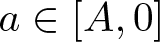 $a\in [A,0]$ we find that
 \begin{equation*}
\beta\left( x_m+ \int_a^t g\left( e^{-\mu \tau} \int_{-\infty}^a e^{\mu s}\phi(s)ds\right) d\tau \right) \gt 0
\end{equation*}
and therefore  $b(t)\geqslant r_\phi(t) \gt 0$ for all
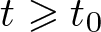 $t\geqslant t_0$.