


1. Introduction
Agricultural intensification poses substantial risks to water and soil resources, contributing to broader environmental degradation (Krupek et al., Reference Krupek, Redfearn, Eskridge and Basche2022). Physical disturbances, such as tillage, typically lead to a decrease in soil aggregate stability and soil erosion (Alhameid et al., Reference Alhameid, Ibrahim, Kumar, Sexton and Schumacher2017; Xue et al., Reference Xue, Wang, Zhao, Sun and Wang2022). A historical example is the Dust Bowl of the 1930s, when intensive tillage combined with prolonged drought led to widespread topsoil loss (Baveye et al., Reference Baveye, Rangel, Jacobson, Laba, Darnault, Otten and Camargo2011; Lal et al., Reference Lal, Reicosky and Hanson2007). The severity of this event emphasized the importance of soil conservation and contributed to the establishment of the Soil Conservation Service, later renamed the Natural Resources Conservation Service (NRCS). Government agencies such as NRCS offer ongoing technical and financial assistance to agricultural producers on soil conservation practices. These efforts help maintain soil health and productivity while also making farms more resilient to extreme weather events such as drought (Aglasan et al., Reference Aglasan, Rejesus, Hagen and Salas2023; Kaye and Quemada, Reference Kaye and Quemada2017).
In this context, conservation tillage practices, particularly no-till farming, have been widely promoted as an effective approach to achieve sustainable agriculture. By eliminating mechanical tillage and retaining crop residues on the soil surface, no-till improves soil structure, reduces erosion, enhances water infiltration, and increases soil organic carbon sequestration (Blanco-Canqui and Ruis, Reference Blanco-Canqui and Ruis2018; Francaviglia et al., Reference Francaviglia, Di Bene, Farina and Salvati2017; Lal, Reference Lal2015; Ogle et al., Reference Ogle, Alsaker, Baldock, Bernoux, Breidt, McConkey and Vazquez-Amabile2019; Sun et al., Reference Sun, Zeng, Shi, Pan and Huang2015). These benefits are complemented by potential cost savings from reduced fuel, labor, and machinery use (Che et al., Reference Che, Rejesus, Cavigelli, White, Aglasan, Knight, Dell, Hollinger and Lane2023; Ogieriakhi and Woodward, Reference Ogieriakhi and Woodward2022), leading many proponents to argue that no-till can enhance both environmental and economic outcomes.
Despite its benefits, the adoption of no-till farming in the US has remained relatively limited in recent years. According to the 2022 Census of Agriculture, only 27.5% of US cropland is currently managed under no-till, a modest increase from 26.3% in 2017 and 24.8% in 2012 (USDA-NASS, 2024). In addition, evidence reveals substantial variability across both crops and regions. At a disaggregated level, no-till adoption has been most prevalent for wheat, which experienced significant early growth from 2004 to 2009; soybean also saw widespread adoption between 2002 and 2006 (Sawadgo and Plastina, Reference Sawadgo and Plastina2022). However, growth in no-till practices slowed for wheat between 2009 and 2017 and declined for soybean between 2006 and 2012; for corn, no-till adoption has grown more modestly and steadily over the same period (Sawadgo and Plastina, Reference Sawadgo and Plastina2022).
Regional patterns mirror these crop-level differences. County-level data from the USDA Economic Research Service (ERS) show that no-till and related conservation practices are concentrated in specific sub-regions, often influenced by agroecological factors such as slope, soil erosion risk, and water availability (Wallander et al., Reference Wallander, Claassen and Bowman2021). For example, higher adoption rates are found in parts of the Mid-Atlantic and southeastern US, where conservation incentives and environmental regulations (e.g., in the Chesapeake Bay watershed) are more prominent. In contrast, adoption remains patchier in the Corn Belt and western regions, where cropping systems and conservation support structures differ (Wallander et al., Reference Wallander, Claassen and Bowman2021).
The slow growth in no-till adoption over the past decade raises the need for investigation into the economic factors shaping farmers’ decisions. Prokopy et al. (Reference Prokopy, Floress, Arbuckle, Church, Eanes, Gao and Singh2019) offer a comprehensive review of the drivers of conservation practice adoption, concluding that farmers are more likely to adopt when a practice improves profitability or crop yields. Similarly, Liu et al. (Reference Liu, Bruins and Heberling2018) emphasize the role of expected income gains and financial incentives in motivating the adoption of new management practices. A recent study by Blackwell et al. (Reference Blackwell, Mitchell-McCallister, Kang, Johnson and Hudson2025) found that producers consistently ranked economic viability as the most difficult dimension of sustainability, and their estimated willingness-to-accept indicated that financial incentives were necessary to encourage participation in sustainability programs. These findings suggest that a detailed, site-specific analysis of the long-term economic impacts of no-till is essential to inform farmer decision-making and guide policy efforts aimed at encouraging broader adoption.
Agronomic conditions can also affect the long-term economic tradeoffs farmers face when considering no-till adoption. Concerns about soil compaction under continuous no-till have led some producers to rely on strip tillage or occasional deep tillage to manage hardpan formation (Nunes et al., Reference Nunes, Denardin, Pauletto, Faganello and Pinto2015). As a result, some producers view alternatives to continuous no-till as a practical adjustment rather than a departure from conservation-oriented management. At the same time, the long-run success of no-till systems depends critically on effective herbicide-based weed control. Increasing resistance to commonly used herbicides, including glyphosate, has raised concerns among both current and prospective no-till adopters about the durability and cost of weed management in corn and soybean systems (Perry et al., Reference Perry, Moschini and Hennessy2016; Van Deynze et al., Reference Van Deynze, Villas-Boas and Hennessy2022). As resistance has spread across major production regions, producers face fewer effective chemical options, increasing uncertainty about long-run weed control strategies.
This study aims to evaluate the long-term economic impacts of no-till adoption relative to conventional tillage, using more than 30 years of experimental field data from three locations: Hoytville, Ohio; Wooster, Ohio; and Hickory Corners, Michigan. These sites differ in soil type and drainage characteristics, providing a useful range of agroecological conditions. The Ohio experiments include continuous observations of corn (Zea mays L.) and soybean (Glycine max L.) from 1982 to 2012, while the Michigan site includes corn, soybean, and wheat (Triticum aestivum L.) from 1989 to 2020. Across all sites, the datasets contain detailed plot-level records of crop yields and four input cost categories: seed, field operations, fertilizer, and pesticides. Using these data, we estimate site-specific linear fixed-effects models to identify the marginal effects of no-till adoption on both yields and costs. We then integrate the resulting estimates into a partial budgeting framework to quantify the net monetary gains or losses associated with adopting no-till.
Despite a growing body of research, evidence on the economic performance of no-till remains mixed (Rejesus et al., Reference Rejesus, Aglasan and Connor2025). Much of the literature focuses on yield effects, while relatively fewer studies examine production cost savings or profitability more directly. On the yield side, some studies document early yield penalties under no-till, whereas others report neutral or positive responses depending on crop, region, and years since adoption (Behnke et al., Reference Behnke, Zuber, Pittelkow, Nafziger and Villamil2018; Boomsma et al., Reference Boomsma, Santini, West, Brewer, McIntyre and Vyn2010; Che et al., Reference Che, Rejesus, Cavigelli, White, Aglasan, Knight, Dell, Hollinger and Lane2023; Cooray et al., Reference Cooray, Rejesus, Aglasan, Li and Woodley2023; Cusser et al., Reference Cusser, Bahlai, Swinton, Robertson and Haddad2020; Daigh et al., Reference Daigh, Dick, Helmers, Lal, Lauer, Nafziger and Cruse2018; DeFelice et al., Reference DeFelice, Carter and Mitchell2006; Pittelkow et al., Reference Pittelkow, Liang, Linquist, van Groenigen, Lee, Lundy and van Kessel2014). For example, DeFelice et al. (Reference DeFelice, Carter and Mitchell2006) report that average national yield differences between no-till and conventional tillage were negligible for corn and soybeans, though responses differed by soil drainage and region. Pittelkow et al. (Reference Pittelkow, Liang, Linquist, van Groenigen, Lee, Lundy and van Kessel2014), in a global meta-analysis, estimate an average maize yield reduction under no-till but find that the gap narrows after the initial years of adoption. Using long-term data from the Michigan KBS site examined here, Cusser et al. (Reference Cusser, Bahlai, Swinton, Robertson and Haddad2020) show that yield differences strengthen over time and become more consistently evident only over sufficiently long study durations.
Evidence on costs and profitability is more limited. Karlen et al. (Reference Karlen, Kovar, Cambardella and Colvin2013), based on a 30-year Iowa experiment, find comparable yields between no-till and chisel plow, with economic gains driven primarily by lower machinery costs. Che et al. (Reference Che, Rejesus, Cavigelli, White, Aglasan, Knight, Dell, Hollinger and Lane2023) use plot-level experimental data from 1996 to 2019 in Maryland to evaluate the long-term financial effects of no-till. They find significantly higher net returns under no-till than under conventional tillage, with the profitability advantage driven mainly by lower field operation costs.
Our empirical strategy employs fixed-effects models that allow the effect of no-till to vary by site, accounting for long-term experimental control and location-specific agronomic dynamics. We then incorporate these estimates into a partial budgeting framework to calculate the net profitability of no-till adoption. This approach enables us to distinguish between gains arising from yield increases and those due to cost savings, two aspects with different implications for adoption behavior.
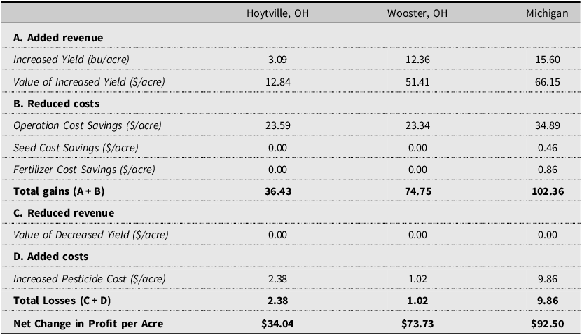
Our findings demonstrate that the economic returns to no-till are site-specific. At the Michigan site, compared to chisel tillage, no-till produces large and statistically significant yield gains (+15.6 bu/ac for corn and + 5.9 bu/ac for soybean), along with substantial reductions in field operation costs (−$34.9/ac for corn and −$38.2/ac for soybean). These effects imply positive net returns of approximately $93 per acre for corn and $86 per acre for soybean. At the Ohio sites, results are more heterogeneous. At Wooster, no-till produces a statistically significant increase in corn yield (+12.4 bu/ac), while the soybean yield effect is positive (+3.6 bu/ac) but not statistically significant. The corresponding net returns are approximately $74 and $59 per acre, respectively. At Hoytville, the yield effect is statistically significant for corn (+3.1 bu/ac) but not for soybean, and profitability gains of approximately $34 per acre for corn and $30 per acre for soybean are driven primarily by reductions in field operation costs. These results suggest that the uneven national adoption of no-till may reflect economically meaningful impacts with location-specific variation.
This study contributes to the economics of soil conservation literature by providing a detailed, site-specific analysis of the long-term economic effects of no-till practices in the US Midwest. Unlike much of the existing research, which often isolates specific outcomes such as crop yields, fuel use, or labor inputs, our analysis considers both yield changes and disaggregated input cost differences, including seed, field operations, fertilizer, and pesticides. Using a rich dataset from more than 30 years of experimental trials across three sites, this study provides evidence on the long-term profitability of no-till under controlled field conditions. The results indicate that profitability is not uniform across sites and suggest that part of this heterogeneity may be related to underlying site characteristics such as soil drainage and texture. These findings suggest that the long-run economic performance of no-till may vary across environments compared to a more conventional tillage system. While informative, the evidence comes from controlled experimental conditions and may not fully capture the transition costs and other farm-level factors that influence producer adoption.
2. Site description, experimental design, and data
This study utilizes data from three long-term tillage experiments, each located in a distinct agroecological setting. The Hoytville site in northwest Ohio (41°00′ N, 84°00′ W) is dominated by Hoytville silty clay loam. These soils are poorly drained and formed from glacial-lacustrine deposits on a flat lake plain. The site has a mean annual temperature of 9.9 °C (49.8 °F) (Mestelan et al., Reference Mestelan, Smeck, Sprunger, Dyck and Dick2021; Soil Survey Staff, 2016). The Wooster site, located in northeast Ohio (40°48′ N, 82°00′ W), contains Wooster silt loam, which is moderately well-drained and developed from glacial till with a loess cap. The mean annual temperature at Wooster is 9.1 °C (48.4 °F) (Soil Survey Staff, 2011). The third site, in Hickory Corners, Michigan (42°24′ N, 85°24′ W), includes both Kalamazoo loam and Oshtemo sandy loam. These soils are moderately well-and well-drained, respectively, and formed from glacial till and outwash deposits on moraines and outwash plains. The average temperature at this site is 9.2 °C (48.6 °F) (Soil Survey Staff, 2015, 2017).
The Ohio datasets are derived from the Triplett-Van Doren Tillage and Crop Rotation Experiments, initiated in 1962 (Wooster) and 1963 (Hoytville) (Dick et al., Reference Dick, Van Doren, Triplett and Henry1986a, Reference Dick, Van Doren, Triplett and Henry1986b; de Camargo Santos et al., Reference de Camargo Santos, Culman and Deiss2025). Both use a two-way factorial design with three tillage systems, no-till, chisel plow, and moldboard plow, and three crop rotations.Footnote 1 Each site employs a randomized complete block design with three replications per treatment. In any given year, each plot grows only one crop, but all crops planted at the Ohio sites (corn and soybean) are represented annually across the rotation. Tillage occurs in the fall at Hoytville and in the spring at Wooster. Secondary tillage operations for moldboard and chisel treatments include disking, harrowing, and cultivation. Treatments have remained largely consistent since the experiments began, with only minor modifications (Dick et al., Reference Dick, Triplett and Van Doren2013).
The Michigan dataset comes from the W.K. Kellogg Biological Station (KBS) Long-Term Ecological Research (LTER) site (Robertson and Hamilton, Reference Robertson, Hamilton, Robertson and Hamilton2015), specifically the Main Cropping System Experiment. This experiment, which began in 1989, uses a randomized complete block design with six replications and includes many treatments, one of which compares a continuous no-till system to a conventional chisel plow system. The crop rotation includes corn, soybean, and winter wheat, with one crop grown per plot per year.
Each Ohio site employs a factorial design with three tillage systems (no-till, chisel, and moldboard) and two crops, replicated three times, resulting in 18 plots per site-year (3 × 2 × 3). The Michigan site includes multiple tillage and management treatments within a corn-soybean-wheat rotation, each replicated six times per crop. For our analysis, we restrict the Michigan sample to two treatments (T1 and T2) that follow the same chemical input management: conventional (chisel) tillage and continuous no-till. We note that “chisel” tillage may contain a range of residue levels and tillage intensities across sites. Because our dataset does not differentiate finer chisel tillage intensity categories, some within-category heterogeneity may remain.Footnote 2 This variation could decrease the estimated no-till benefits if “chisel” in Michigan is already more conservative than “chisel” in Ohio.
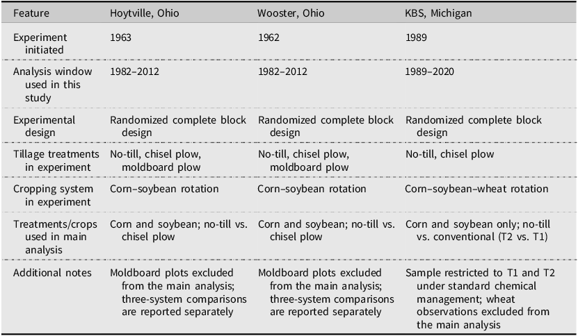
Table 1 provides a summary of the three experimental sites, their design features, and the restrictions used to define the analytical sample in the main analysis. We exclude observations from the moldboard plow treatment at the Ohio sites to maintain consistency with the Michigan site, for which we only used treatments that compare no-till and chisel tillage systems. In addition, wheat observations from the Michigan site are excluded from the pooled cross-site analysis to maintain comparability with the Ohio corn-soybean systems. The resulting sample includes corn and soybean data under no-till and chisel tillage systems across the three sites, with six plots per crop per year at each Ohio site and eight plots per crop per year at the Michigan site. It is also worth noting that although the Ohio experimental trials were established in 1962–1963, our analysis begins in 1982, as detailed input cost data were not available during the first two decades of the experiment.
Summary of experimental sites, design, and analytical sample

Table 1. Long description
The table compares features of three experimental sites in Hoytville, Ohio, Wooster, Ohio, and KBS, Michigan. It has seven rows and four columns, including the headers. The columns are labeled Feature, Hoytville, Ohio, Wooster, Ohio, and KBS, Michigan. The rows are labeled Experiment initiated, Analysis window used in this study, Experimental design, Tillage treatments in experiment, Cropping system in experiment, Treatments/crops used in main analysis, and Additional notes. Row 1: Experiment initiated, 1963, 1962, 1989. Row 2: Analysis window used in this study, 1982-2012, 1982-2012, 1989-2020. Row 3: Experimental design, Randomized complete block design, Randomized complete block design, Randomized complete block design. Row 4: Tillage treatments in experiment, No-till, chisel plow, moldboard plow, No-till, chisel plow, moldboard plow, No-till, chisel plow. Row 5: Cropping system in experiment, Corn-soybean rotation, Corn-soybean rotation, Corn-soybean-wheat rotation. Row 6: Treatments/crops used in main analysis, Corn and soybean; no-till vs. chisel plow, Corn and soybean; no-till vs. chisel plow, Corn and soybean only; no-till vs. conventional (T2 vs. T1). Row 7: Additional notes, Moldboard plots excluded from the main analysis; three-system comparisons are reported separately, Moldboard plots excluded from the main analysis; three-system comparisons are reported separately, Sample restricted to T1 and T2 under standard chemical management; wheat observations excluded from the main analysis.
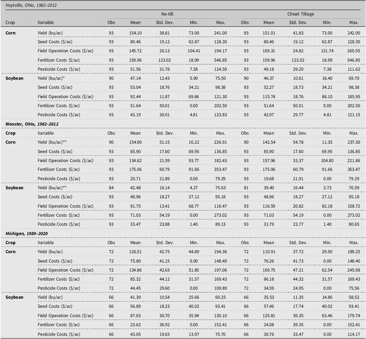
Descriptive statistics by site, crop, and tillage system are presented in Table 2, and additional details on cost variable construction are provided in Appendix A. For our analysis, we examine the effects on yield and four categories of input costs: seed, field operations, fertilizer, and pesticides. Field operations include all mechanical activities, from tillage and planting to spraying and harvest, and are valued using per-acre custom rates reported by Michigan State University and Ohio State University for the relevant operations in each state. Fertilizer costs account for nitrogen (N), phosphate (P2O5), potash (K2O), and lime. At the Ohio sites, fertilizer and seed inputs were applied uniformly across tillage treatments within each crop-year-block, resulting in no systematic cost differences. Pesticide costs include herbicides and insecticides, such as 2,4-D, glyphosate, and metribuzin.Footnote 3
Descriptive statistics of crop yield and input costs by tillage system across experimental sites

Table 2. Long description
The table presents descriptive statistics of crop yield and input costs for different tillage systems across three sites: Hoytville, Ohio; Wooster, Ohio; and Michigan. The table is divided into sections for each site, with data for corn and soybean crops under no-till and chisel tillage systems. Each section includes variables such as yield, seed costs, field operation costs, fertilizer costs, and pesticide costs. The table provides observations, mean, standard deviation, minimum, and maximum values for each variable. For example, in Hoytville, Ohio, the corn yield under no-till has a mean of 154.10 bu/ac with a standard deviation of 38.81, while under chisel tillage, the mean yield is 151.01 bu/ac with a standard deviation of 41.83. Similar detailed statistics are provided for soybean crops and other sites.
Notes: All monetary values are expressed in real 2024 dollars.
At both the Ohio and Michigan sites, pesticide use reflects the weed management strategy inherent to each tillage system. No-till plots rely more heavily on chemical control, requiring herbicide applications to terminate weeds prior to planting, whereas conventionally tilled plots incorporate mechanical disturbance as part of weed management. This substitution between chemical and mechanical control represents differences in operation management between the systems and explains the observed differences in pesticide and field operation costs. Note that at the Michigan site, the analysis is restricted to treatments that follow the same chemical input management under the same crop rotation. Fertilizer and seeding recommendations are therefore comparable across systems. Any cost differences reflect differences in management practices and not structurally different input regimes.
To ensure comparability across the more than 30-year study period, all monetary values are converted to real 2024 dollars using the Consumer Price Index for All Urban Consumers (CPI-U) published by the U.S. Bureau of Labor Statistics. This adjustment accounts for cumulative inflation over the sample period and allows cost savings and revenue changes to be compared in constant purchasing power.
3. Empirical approach
3.1. Estimation strategy
To quantify the site-specific effects of no-till adoption on crop yields and input costs, we estimate a fixed-effects regression model that accounts for treatment variation across heterogeneous field environments. Recognizing that the agronomic and economic impacts of conservation tillage may depend on local conditions, our specification allows the effect of no-till to vary by site. We estimate the model separately for corn and soybean outcomes. The equation is given by:
 \[{y_{ibst}} = \sum\nolimits_s {{\beta _s}} \;\left( {N{T_{ibst}} \times 1\left\{ {Site = s} \right\}} \right) + {\delta _b} + {\lambda _{st}} + {\varepsilon _{ibst}}\]
where y ibst represents the outcome for plot i, in block b, at site s, in year t. The outcome variable includes yield (in bu/ac) or input costs (in $/ac) for seed, field operations, fertilizer, or pesticides. The indicator variable NT ibst equals one if the plot is managed under no-till and zero if it is managed using chisel tillage. The term 1{Site = s} is an indicator for site s, so that β s captures the site-specific effect of no-till across Hoytville, Wooster, and Michigan. The term δ t denotes block fixed effects, which control for time-invariant differences across experimental blocks, and λ st denotes site-by-year fixed effects, which absorb shocks common to all plots within a given site and year. Lastly, the error term is denoted by ϵ ibst .
3.2. Statistical inference and standard errors
To account for the panel structure of the experimental data, in which observations within plots may be correlated over time, we rely on cluster-robust variance estimation as our primary inference strategy with alternative clustering and randomization inference as robustness checks. Our baseline estimates use cluster-robust standard errors clustered at the plot level, implemented with the bias-reduced linearization (CR2) variance estimator (Pustejovsky and Tipton, Reference Pustejovsky and Tipton2017). Plot-level clustering addresses serial correlation within experimental plots. The CR2 estimator is designed for settings with a modest number of clusters and provides improved finite-sample performance relative to conventional cluster-robust estimators. As a sensitivity check, we re-estimate all models clustering standard errors by year. Year-level clustering accounts for potential correlation across plots within the same year, such as common weather shocks or management decisions made at the experimental station level.
Given the experimental nature of the data, we also implement randomization inference (RI) as a non-asymptotic alternative to cluster-robust inference (Athey and Imbens, Reference Athey and Imbens2017; Young, Reference Young2018). Treatment assignment was randomized within site–crop–replication blocks at the start of the experiment and remained fixed over time. Randomization inference generates finite-sample p-values by comparing the observed treatment effect to the distribution obtained under repeated permutations of the original treatment assignment. For each outcome, we conduct 1,000 permutations within each site-crop combination, re-estimate the regression under each permutation, and compute the proportion of permuted test statistics that are at least as extreme as the observed statistic. Our analysis evaluates the effects of no-till on five outcomes (yield and four input costs) across three sites and two crops, resulting in a total of 30 hypothesis tests. To address concerns related to multiple testing, we control the false discovery rate (FDR) using the Benjamini–Hochberg procedure (Benjamini and Hochberg, Reference Benjamini and Hochberg1995), applied within each crop-outcome pair at a p-value threshold of 0.10.
3.3. Partial budgeting analysis
Adopting a new management practice is a significant decision for farmers, requiring careful consideration of various factors, with economic viability being among the most critical. Therefore, we conduct a partial budgeting analysis to quantify the financial implications of adopting no-till. Partial budgeting is a standard farm management tool that isolates the economic effects of a proposed change by focusing only on components that differ between systems (Cornelisse and Hyde, Reference Cornelisse and Hyde2013; Kay et al., Reference Kay, Edwards and Duffy2016).
Using the marginal effects estimated from the linear fixed-effects models, we calculate expected changes in net returns per acre ($/ac) associated with no-till adoption relative to chisel tillage. Potential sources of profitability gains include changes in yield and reductions in input costs. Yield effects are monetized using 2024 harvest prices obtained from the USDA Risk Management Agency’s Price Discovery Tool, based on December Chicago Board of Trade contracts. Specifically, we use a corn price of $4.16/bu for Ohio and $4.24/bu for Michigan and a soybean price of $10.03/bu for both states.Footnote 4 By breaking down the economic effects into specific components, partial budgeting analysis offers a straightforward view of how no-till adoption influences profits. Our main budget analysis uses the full set of estimated coefficients from the regression models to calculate per-acre changes in net returns from adopting no-till relative to chisel tillage.Footnote 5
Because the purpose of the partial budgeting exercise is to evaluate the profitability effect of no-till under a common price environment, the estimated yield effects must be valued using a single set of output prices, which imposes a single-price-year assumption. To examine whether the results depend on that assumption, we also estimate treatment effects directly on realized net profit per acre using actual historical prices and report additional partial budget results under alternative price scenarios.
As a supplementary exercise, we calculate the break-even transition cost implied by the estimated annual net return from no-till. For each site-crop combination, let Δπ denote the annual net change in returns based on the partial budgeting analysis, then the break-even upfront cost over a planning horizon of T years at discount rate r is
 ${\rm BE}=\Delta \pi \times {1-\left(1+r\right)^{-T} \over r}.$
This amount represents the maximum one-time cost per acre a producer could incur and still break even on no-till adoption over a given planning horizon.
3.4. Robustness checks and sensitivity analyses
We implement several robustness checks to assess the validity and sensitivity of our results.Footnote 6 We re-estimate standard errors clustered at the year level. This approach allows for arbitrary correlation in shocks across observations within the same year, providing a more conservative test of statistical significance when unobserved factors are shared over time. In addition, we estimate the model using only data from the Ohio sites, where all three tillage systems, no-till, chisel, and moldboard, were implemented under a common experimental structure. This allows us to compare no-till against both conventional tillage systems and evaluate whether the exclusion of moldboard plots from the main analysis influences the results. For the Michigan site, we extend the analysis to include wheat in the crop rotation. Wheat is omitted from the primary cross-site comparison to maintain comparability with the Ohio corn-soybean systems, but including it provides a more complete picture of profitability within the Michigan rotation. These expanded specifications allow us to assess whether the main findings are sensitive to the choice of comparison tillage system or to the exclusion of additional crops included in the full experimental design. Lastly, we examine the stability of treatment effects over time by partitioning the data into site-specific decade-long periods. This time-split analysis allows us to assess whether the economic effects of no-till differ across periods, which may reflect changes in environmental conditions, input technologies, or management practices.
4. Empirical results
4.1. Descriptive evidence
A visual inspection of the raw data provides preliminary evidence of heterogeneous effects of no-till adoption across the three experimental sites. Figure 1(a) plots the annual yield difference between no-till and chisel tillage for both corn and soybean. At the Michigan site, no-till consistently outperforms chisel tillage for corn, with yield differences generally larger in later years. Soybean yield differences in Michigan also favor no-till, though with greater year-to-year variability. In contrast, the plotted yield differences at the Ohio sites fluctuate around zero without a clear long-run trend for both crops, especially for the Hoytville site. Figure 1(b) presents annual differences in field operation costs between the two systems. Across all sites and both crops, no-till is associated with lower operation costs. The cost savings are most pronounced at Wooster, particularly for corn in later years. In Hoytville and Michigan, no-till also reduces operation costs, though the magnitude is smaller and exhibits less pronounced variation over time.
(a). Annual yield differences between no-till and chisel tillage by site and crop (bu/acre). (b). Annual field operation cost differences between no-till and chisel tillage by site and crop ($/acre).

Summary statistics reported in Table 2 are consistent with these patterns. For corn, the largest average yield difference in favor of no-till occurs in Michigan, while differences at the Ohio sites are smaller. For soybean, the average yield difference is again the largest in Michigan, with more modest differences in Ohio. Field operation costs are consistently lower under no-till across sites, whereas other input costs display greater variability. These descriptive comparisons do not account for time trends or site-specific fixed effects and therefore serve only as preliminary evidence, motivating the regression analysis that follows.
4.2. Regression results
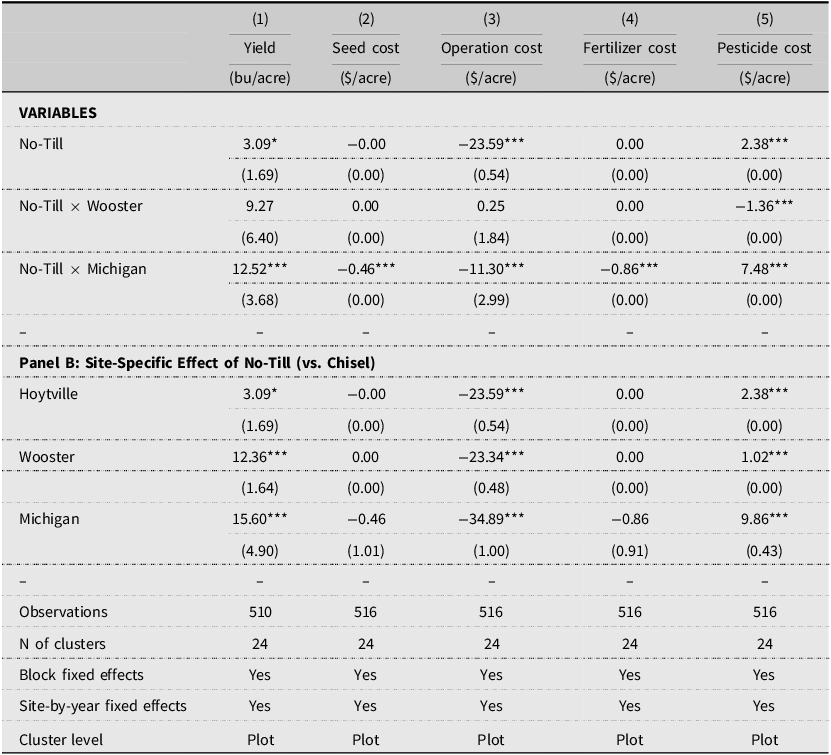
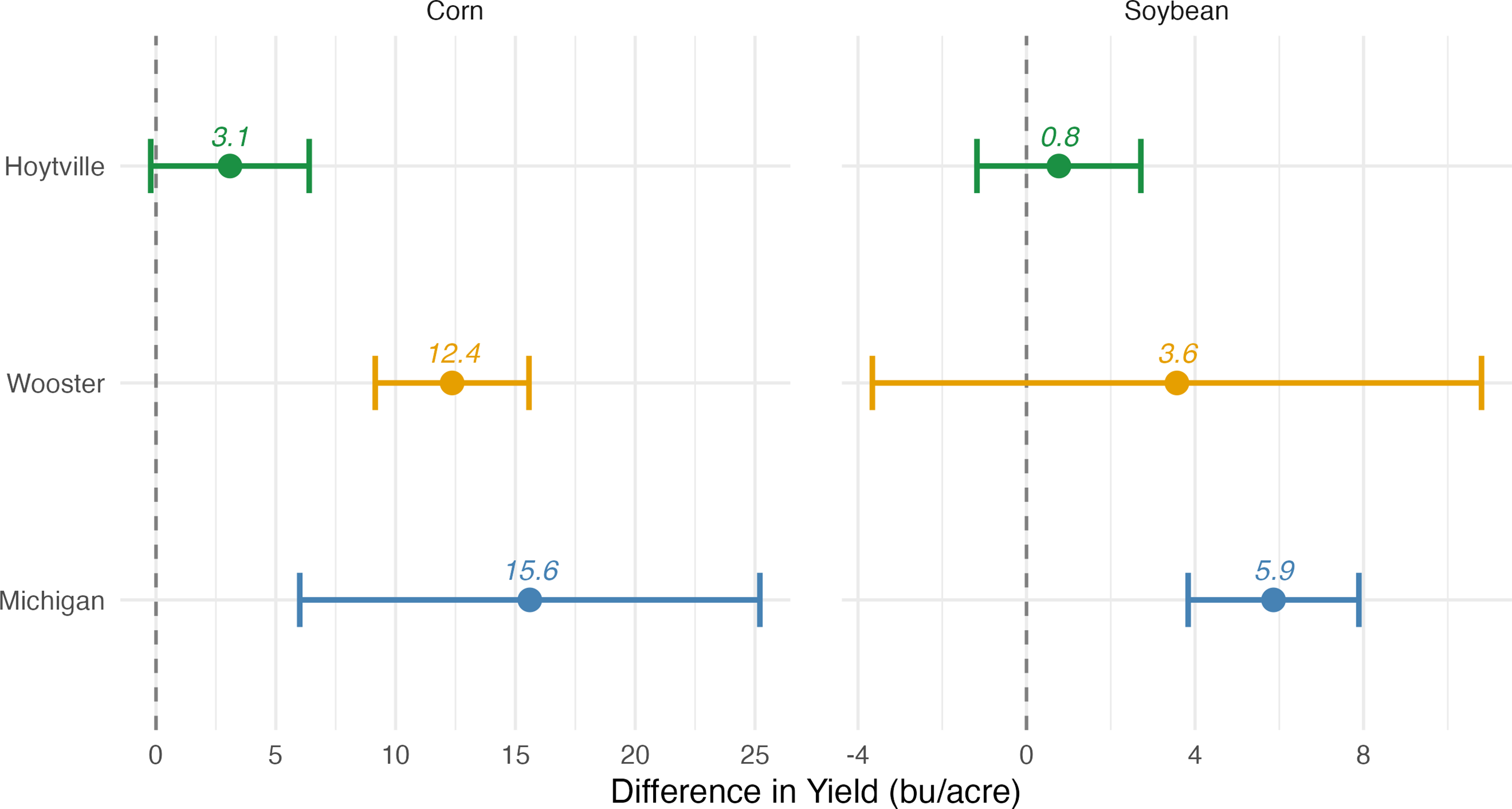
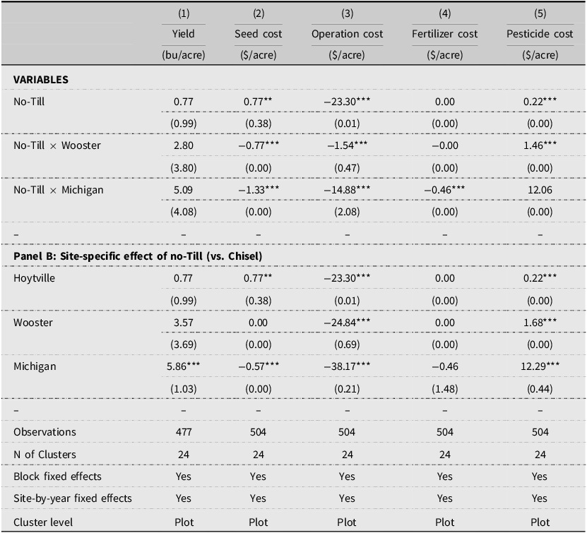
Regression results for yield and input costs are reported in Table 3 for corn and Table 5 for soybean. Site-specific yield effects are also visualized in Figure 2, which presents estimated yield differences between no-till and chisel tillage with 95% confidence intervals. The economic effects of no-till differ substantially across sites and crops.
The effect of no-till adoption on corn yield and input costs

Table 3. Long description
The table compares the effects of no-till farming on corn yield and input costs across different sites. It has two main sections: Panel A and Panel B. Panel A shows the overall variables affecting yield, seed cost, operation cost, fertilizer cost, and pesticide cost. Panel B details the site-specific effects of no-till versus chisel tillage. The table includes data for Hoytville, Wooster, and Michigan. Each row lists specific variables and their corresponding values. For example, No-Till shows a yield of 3.09 bu/acre, a seed cost of -0.00 $/acre, an operation cost of -23.59 $/acre, a fertilizer cost of 0.00 $/acre, and a pesticide cost of 2.38 $/acre. The table also includes statistical observations, the number of clusters, block fixed effects, site-by-year fixed effects, and the cluster level.
Notes: The table reports site-specific effects of no-till adoption relative to chisel tillage, for corn. The dependent variable for each column is listed at the top of the table. Robust standard errors clustered at the plot level are reported in parentheses. All monetary values are expressed in real 2024 dollars. Ohio sites span 1982–2012, and Michigan spans 1989-2020. Significance stars denote p-values: *** p < 0.01, ** p < 0.05, * p < 0.10.
Estimated effects of no-till on crop yield relative to Chisel Tillage (bu/acre).

Figure 2. Long description
The image contains two side-by-side bar graphs comparing the estimated effects of no-till on crop yield relative to chisel tillage for corn and soybean in different locations. Panel A: The left graph shows the difference in yield for corn. The horizontal axis represents the difference in yield in bushels per acre, ranging from 0 to 25. The vertical axis lists three locations: Hoytville, Wooster, and Michigan. Each location has a bar with an error bar indicating the estimated effect and its uncertainty. Hoytville shows a yield difference of 3.1 bushels per acre, Wooster shows 12.4 bushels per acre, and Michigan shows 15.6 bushels per acre. Panel B: The right graph shows the difference in yield for soybean. The horizontal axis represents the difference in yield in bushels per acre, ranging from -4 to 8. The vertical axis lists the same three locations: Hoytville, Wooster, and Michigan. Each location has a bar with an error bar indicating the estimated effect and its uncertainty. Hoytville shows a yield difference of 0.8 bushels per acre, Wooster shows 3.6 bushels per acre, and Michigan shows 5.9 bushels per acre.
For corn, the largest yield effect appears in Michigan, where no-till increases yield by 15.60 bu/ac (p < 0.01). In Ohio, the estimated yield gain is smaller but still statistically significant at Hoytville (3.1 bu/ac, p = 0.07) and larger at Wooster (12.4 bu/ac, p < 0.01). Operation cost savings are statistically significant at all three sites and are economically meaningful, with the largest savings observed in Michigan (−$34.9/ac). No-till is also associated with higher pesticide costs, consistent with greater reliance on chemical inputs relative to conventional tillage. Seed and fertilizer cost differences are statistically insignificant.
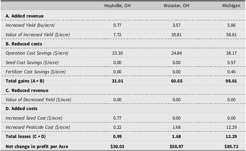
For soybean, the largest yield gain again appears in Michigan, where no-till raises yield by 5.86 bu/ac (p < 0.01). The two Ohio sites show positive soybean yield effects of 0.77 bu/ac at Hoytville and 3.57 bu/ac at Wooster, but neither estimate is statistically significant. Operation cost savings are present at all three sites and are statistically significant in each site. Similar to corn, no-till soybean production is also associated with increases in pesticide costs. Effects on seed and fertilizer costs are mostly statistically insignificant, and where they are significant, the magnitudes are generally small.
4.3. Summary of economic returns
The partial budgeting results are summarized in Tables 4 and 6. In Michigan, yield gains and operation cost savings combine to generate large net return increases, approximately $93 per acre for corn and $86 per acre for soybean. At Wooster, profitability also reflects contributions from both yield gains and operation cost savings, though the yield component is smaller than in Michigan. At Hoytville, by contrast, net return gains are driven primarily by field operation cost savings. Across the Ohio sites, net returns range from approximately $34 to $74 per acre for corn and from $30 to $59 per acre for soybean. Figure 3 decomposes the net change in profits from no-till adoption by site and crop, where the stacked bars illustrate the relative contributions of yield-related revenue gains and cost savings to overall profitability at each site.Footnote 7
Partial budget analysis of adopting no-till for corn , changes in profit relative to chisel tillage ($/acre)

Table 4. Long description
The table presents a partial budget analysis of adopting no-till for corn, showing changes in profit relative to chisel tillage in dollars per acre across different locations. It has 4 rows and 3 columns. The columns are labeled Hoytville, OH, Wooster, OH, and Michigan. The rows are labeled with different categories and subcategories. Row 1: Added revenue. Row 2: Increased Yield (bu/acre) with values 3.09, 12.36, 15.60. Row 3: Value of Increased Yield ($/acre) with values 12.84, 51.41, 66.15. Row 4: Reduced costs. Row 5: Operation Cost Savings ($/acre) with values 23.59, 23.34, 34.89. Row 6: Seed Cost Savings ($/acre) with values 0.00, 0.00, 0.46. Row 7: Fertilizer Cost Savings ($/acre) with values 0.00, 0.00, 0.86. Row 8: Total gains (A+B) with values 36.43, 74.75, 102.36. Row 9: Reduced revenue. Row 10: Value of Decreased Yield ($/acre) with values 0.00, 0.00, 0.00. Row 11: Added costs. Row 12: Increased Pesticide Cost ($/acre) with values 2.38, 1.02, 9.86. Row 13: Total Losses (C+D) with values 2.38, 1.02, 9.86. Row 14: Net Change in Profit per Acre with values 34.04, 73.73, 92.50.
Notes: This table calculates the net change in profit from adopting no-till over chisel tillage, using point estimates from the regression results in Table 3. Assumed 2024 harvest prices are $4.16/bu for corn in Ohio and $4.24/bu for corn in Michigan, based on the USDA RMA Price Discovery Tool.
The effect of no-till adoption on soybean yield and input costs

Table 5. Long description
The table presents regression results for the effects of no-till farming on soybean yield and input costs. It includes five columns: Yield, Seed cost, Operation cost, Fertilizer cost, and Pesticide cost, each with values for different variables and sites. The variables include No-Till, No-Till x Wooster, and No-Till x Michigan. Panel B provides site-specific effects of no-till versus chisel tillage for Hoytville, Wooster, and Michigan. Each row lists specific values for yield and costs, with observations, clusters, fixed effects, and cluster levels detailed at the bottom.
Notes: The table reports site-specific effects of no-till adoption relative to chisel tillage, for soybean. The dependent variable for each column is listed at the top of the table. Robust standard errors clustered at the plot level are reported in parentheses. All monetary values are expressed in real 2024 dollars. Ohio sites span 1982–2012, and Michigan spans 1989-2020. Significance stars denote p-values: *** p < 0.01, ** p < 0.05, * p < 0.10.
Partial budget analysis of adopting no-till for soybean , changes in profit relative to chisel tillage ($/acre)

Table 6. Long description
A table comparing the financial impact of adopting no-till for soybean in Hoytville, OH, Wooster, OH, and Michigan. The table has 4 rows and 3 columns. Column headers are Hoytville, OH, Wooster, OH, and Michigan. Row labels are Increased Yield (bu/acre), Value of Increased Yield ($/acre), Operation Cost Savings ($/acre), Seed Cost Savings ($/acre), Fertilizer Cost Savings ($/acre), Total gains (A+B), Value of Decreased Yield ($/acre), Increased Seed Cost ($/acre), Increased Pesticide Cost ($/acre), Total losses (C+D), and Net change in profit per Acre. Row 1: Increased Yield (bu/acre), Hoytville, OH, 0.77; Wooster, OH, 3.57; Michigan, 5.86. Row 2: Value of Increased Yield ($/acre), Hoytville, OH, 7.72; Wooster, OH, 35.81; Michigan, 58.81. Row 3: Operation Cost Savings ($/acre), Hoytville, OH, 23.30; Wooster, OH, 24.84; Michigan, 38.17. Row 4: Seed Cost Savings ($/acre), Hoytville, OH, 0.00; Wooster, OH, 0.00; Michigan, 0.57. Row 5: Fertilizer Cost Savings ($/acre), Hoytville, OH, 0.00; Wooster, OH, 0.00; Michigan, 0.46. Row 6: Total gains (A+B), Hoytville, OH, 31.01; Wooster, OH, 60.65; Michigan, 98.01. Row 7: Value of Decreased Yield ($/acre), Hoytville, OH, 0.00; Wooster, OH, 0.00; Michigan, 0.00. Row 8: Increased Seed Cost ($/acre), Hoytville, OH, 0.77; Wooster, OH, 0.00; Michigan, 0.00. Row 9: Increased Pesticide Cost ($/acre), Hoytville, OH, 0.22; Wooster, OH, 1.68; Michigan, 12.29. Row 10: Total losses (C+D), Hoytville, OH, 0.99; Wooster, OH, 1.68; Michigan, 12.29. Row 11: Net change in profit per Acre, Hoytville, OH, 30.03; Wooster, OH, 58.97; Michigan, 85.72.
Notes: This table calculates the net change in profit from adopting no-till over chisel tillage, using point estimates from the regression results in Table 5. Assumed 2024 harvest price of $10.03/bu for soybean for all sites, based on the USDA RMA Price Discovery Tool.
Estimated net change in profit from no-till adoption by site and crop ($/acre).

The differences in magnitude across sites likely reflect differences in management history and experimental timing across locations. The Ohio tillage experiments were initiated in 1962–1963, meaning that roughly two decades of conservation tillage had elapsed before the yield data used in our analysis began. Soil organic matter and associated soil property changes under reduced tillage tend to accumulate gradually and may stabilize over time (West and Post, Reference West and Post2002), so differences between chisel tillage and no-till in Ohio may have narrowed by the start of our sample period. In contrast, the Michigan tillage treatments were established in 1989, and cost data are observed from the beginning of the experiment, allowing the evolution of differences between systems to be observed within the dataset. This interpretation is consistent with evidence from the KBS site. Cusser et al. (Reference Cusser, Bahlai, Swinton, Robertson and Haddad2020), using the same long-term experimental data, show that differences in crop yield between no-till and conventional tillage increase over time and become statistically significant after sufficiently long study durations, suggesting that any yield advantage at this site may develop gradually under sustained no-till management.
As a sensitivity check, Appendix Tables A.3 and A.4 report an alternative partial budget in which statistically insignificant coefficients are set to zero. The largest differences arise at Hoytville, where the insignificant yield effects are removed and the remaining net return gains are driven entirely by operation cost savings. To cross-check on the use of a single price year in the partial budget, we also estimate treatment effects directly on realized net profit per acre using observed historical prices. Appendix Figure A.1 plots the comparison between the yield-based partial budget and the revenue-based net profit effect, and the results are broadly consistent, indicating that the main conclusions are not driven by the price assumption. Appendix Table A.5 reports partial budget results under alternative output price assumptions. Across all price scenarios, the conclusion of positive net returns to no-till remains unchanged.
4.4. Break-even transition cost
To summarize the long-run economic implications of the estimated annual net return gains, we calculate the break-even transition cost implied by the partial budget results using Equation (2). This value is defined as the maximum one-time per-acre transition cost that could be incurred while still breaking even over a given planning horizon. It provides a threshold for interpreting the estimated annual gains, including costs such as specialized equipment, learning, or temporary adjustment losses.
At a 5% real discount rate and a 10-year horizon, the implied break-even transition cost ranges from $232 per acre for soybean at Hoytville to $714 per acre for corn in Michigan. Wooster falls between these values, with break-even thresholds of $569 per acre for corn and $455 per acre for soybean. Extending the planning horizon to 20 years increases the implied thresholds, with a range of $374 per acre for Hoytville soybean and $1,153 per acre for Michigan corn. A more detailed break-even calculation across different horizons is presented in Appendix Table A.6. These results indicate that the estimated annual gains from no-till could justify relatively large one-time transition costs over a longer planning horizon, even though the analysis does not identify actual transition costs faced by producers.
5. Robustness checks results
We examine the robustness of the main results in four dimensions: alternative inference, alternative comparison of tillage systems, alternative crop coverage, and temporal stability. Across these checks, the main findings remain unchanged. Yield responses continue to vary by site, operation cost savings remain persistent, and the implied net profitability of no-till stays positive, implying that the primary results are not driven by the choice of inference approach, time-specific shocks, or choice of comparison tillage system.
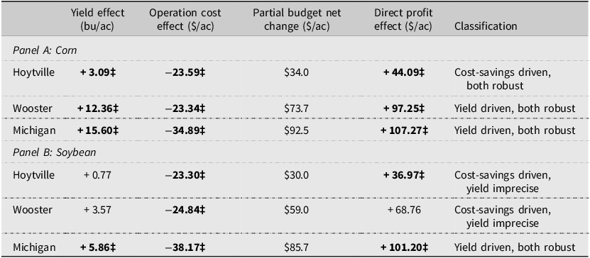
First, we apply year-clustered standard errors to account for potential cross-plot correlation within a given year. Results are presented in Appendix Table A.1. Although standard errors are larger in some cases, the statistical significance and economic interpretation of the main treatment effects are mostly consistent, indicating that our conclusions are not sensitive to the choice of clustering level. In addition, given that our analysis involves a large number of related hypothesis tests, we adjust for multiple testing using an FDR procedure. Appendix Table A.2 reports the resulting comparison between cluster-robust inference and randomization inference after FDR adjustment. Overall, the two approaches agree on every significance decision. Table 7 provides a compact summary of the main economic findings across crops and sites, identifying which estimates remain statistically significant after controlling for FDR. Similar to what we find from the main specification, operation cost savings remain statistically significant across all site-crop combinations, making reduced field operations the most consistent source of economic gains under no-till. Yield effects are more heterogeneous. For corn, the estimated gains remain statistically significant at all three sites, whereas for soybean only the Michigan yield effect remains statistically significant after FDR adjustment.
Summary of no-till effects and false discovery rate (FDR) robust results by crop and site

Table 7. Long description
The table presents a summary of the main economic findings across crops and sites, identifying which estimates remain statistically significant after controlling for false discovery rate. It includes data for corn and soybean across three sites: Hoytville, Wooster, and Michigan. The table has four columns: Yield effect (bu/ac), Operation cost effect ($/ac), Partial budget net change ($/ac), and Direct profit effect ($/ac). It also includes a classification column indicating whether the results are cost-savings driven or yield driven, and whether they are robust. Panel A focuses on corn, and Panel B focuses on soybean. Each panel lists the yield effect, operation cost effect, partial budget net change, direct profit effect, and classification for each site. For corn, Hoytville shows a yield effect of 3.09, an operation cost effect of -23.59, a partial budget net change of 34.0, and a direct profit effect of 44.09, classified as cost-savings driven and robust. Wooster shows a yield effect of 12.36, an operation cost effect of -23.34, a partial budget net change of 73.7, and a direct profit effect of 97.25, classified as yield driven and robust. Michigan shows a yield effect of 15.60, an operation cost effect of -34.89, a partial budget net change of 92.5, and a direct profit effect of 107.27, classified as yield driven and robust. For soybean, Hoytville shows a yield effect of 0.77, an operation cost effect of -23.30, a partial budget net change of 30.0, and a direct profit effect of 36.97, classified as cost-savings driven and yield imprecise. Wooster shows a yield effect of 3.57, an operation cost effect of -24.84, a partial budget net change of 59.0, and a direct profit effect of 68.76, classified as cost-savings driven and yield imprecise. Michigan shows a yield effect of 5.86, an operation cost effect of -38.17, a partial budget net change of 85.7, and a direct profit effect of 101.20, classified as yield driven and robust.
Notes: The symbol ‡ indicates that the estimate is statistically significant at the 10% level after Benjamini–Hochberg FDR adjustment within each outcome group. “Partial budget net change” reports the implied annual change in net returns from the partial budget and is therefore not indicated for statistical significance. “Direct profit effect” reports the treatment effect from the revenue-based regression of realized net profit per acre, calculated using year-specific crop prices. “Classification” provides a qualitative summary of whether profitability is primarily driven by an increase in yield or cost savings. All monetary values are expressed in real 2024 dollars. Full inference results are reported in Appendix Table A.2.
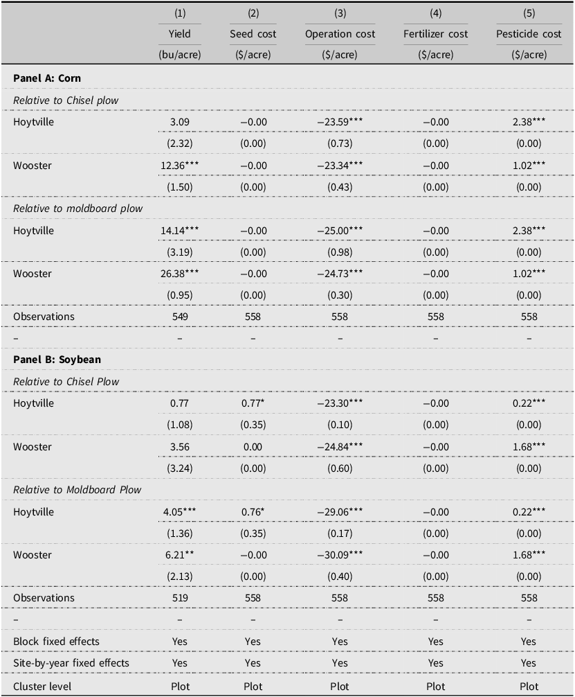
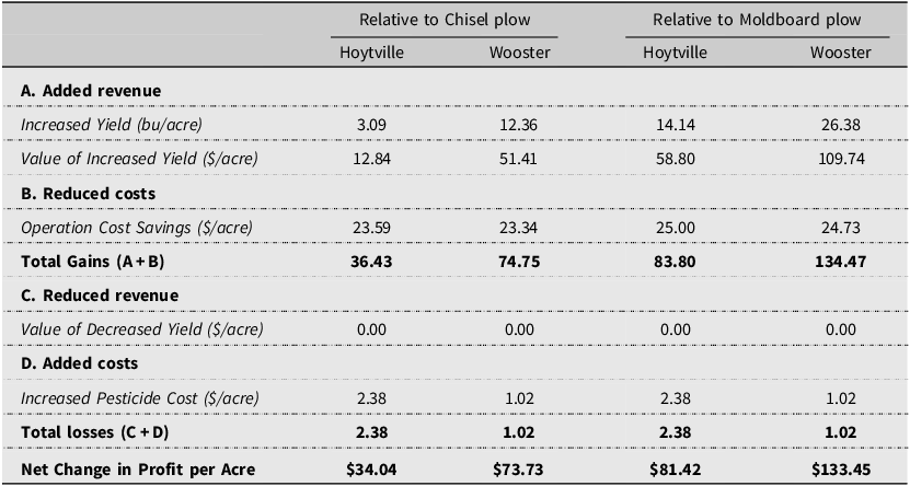
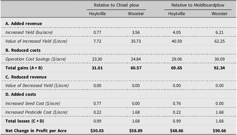
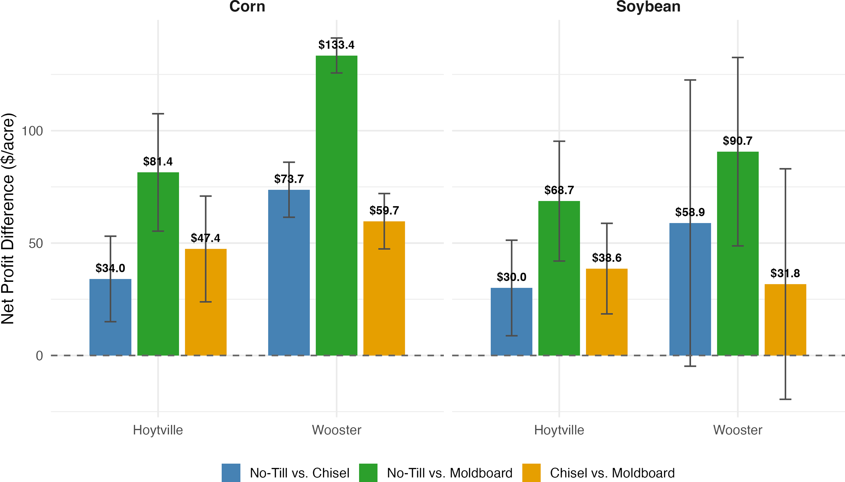
We next examine whether the main results depend on the choice of comparison tillage system. For the Ohio sites, where no-till, chisel, and moldboard were all implemented, we estimate specifications that include all three systems. Results are reported in Table 8, with associated partial budgets in Tables 9 and 10. Relative to chisel tillage, no-till continues to generate statistically significant operation cost savings for both corn and soybean. Relative to moldboard plow, these cost savings are even larger, reflecting the greater field operation intensity of moldboard systems. Compared with the more heterogeneous yield response between no-till and chisel tillage, no-till shows consistently higher yields for both corn and soybean when compared with moldboard tillage. The corresponding partial budgets show that no-till remains more profitable than both chisel and moldboard systems in Ohio. The visualized profit differences across tillage systems for the Ohio sites are shown in Figure 4. Profit gains of no-till relative to moldboard are larger than those relative to chisel, while the direction of economic impact remains consistent across comparison groups. These results indicate that restricting the main analysis to the no-till versus chisel comparison does not overstate the economic performance of no-till.
The effect of adopting no-till on yield and input costs in Ohio, all three tillages

Table 8. Long description
A table comparing the effects of no-till farming on yield and input costs for corn and soybean relative to chisel and moldboard plow systems in Ohio. The table has five columns and multiple rows, including headers and observations. Panel A focuses on corn, while Panel B focuses on soybean. Each panel is further divided into comparisons relative to chisel plow and moldboard plow. Column headers include Yield (bu/acre), Seed cost ($/acre), Operation cost ($/acre), Fertilizer cost ($/acre), and Pesticide cost ($/acre). Row labels include locations (Hoytville and Wooster) and observations. Panel A: Corn. Relative to Chisel plow: Row 1: Hoytville, Yield 3.09, Seed cost -0.00, Operation cost -23.59***, Fertilizer cost -0.00, Pesticide cost 2.38***. Row 2: Wooster, Yield 12.36***, Seed cost -0.00, Operation cost -23.34***, Fertilizer cost -0.00, Pesticide cost 1.02***. Relative to Moldboard plow: Row 3: Hoytville, Yield 14.14***, Seed cost -0.00, Operation cost -25.00***, Fertilizer cost -0.00, Pesticide cost 2.38***. Row 4: Wooster, Yield 26.38***, Seed cost -0.00, Operation cost -24.73***, Fertilizer cost -0.00, Pesticide cost 1.02***. Observations: 549, 558, 558, 558, 558. Panel B: Soybean. Relative to Chisel Plow: Row 5: Hoytville, Yield 0.77, Seed cost 0.77*, Operation cost -23.30***, Fertilizer cost -0.00, Pesticide cost 0.22***. Row 6: Wooster, Yield 3.56, Seed cost -0.00, Operation cost -24.84***, Fertilizer cost -0.00, Pesticide cost 1.68***. Relative to Moldboard Plow: Row 7: Hoytville, Yield 4.05***, Seed cost 0.76*, Operation cost -29.06***, Fertilizer cost -0.00, Pesticide cost 0.22***. Row 8: Wooster, Yield 6.21**, Seed cost -0.00, Operation cost -30.09***, Fertilizer cost -0.00, Pesticide cost 1.68***. Observations: 519, 558, 558, 558, 558. Block fixed effects and Site-by-year fixed effects are included, with the cluster level being Plot.
Notes: This table reports site-specific effects of adopting no-till relative to alternative tillage systems (chisel plow and moldboard plow) for Ohio sites only (Hoytville and Wooster). Each entry represents the total effect of no-till relative to the specified baseline tillage system. Robust standard errors clustered at the plot level are reported in parentheses. All monetary values are expressed in real 2024 dollars. Ohio sites span 1982-2012. Significance stars denote p-values: *** p < 0.01, ** p < 0.05, * p < 0.10.
Partial budget analysis for adopting no-till for corn in Ohio, changes in profit relative to conventional tillage systems ($/acre)

Table 9. Long description
A table comparing profit changes for adopting no-till farming relative to chisel and moldboard plows in Ohio. The table has 10 rows and 6 columns. The columns are labeled: Relative to Chisel plow, Relative to Moldboard plow, Hoytville, Wooster, Hoytville, Wooster. The rows are labeled: Added revenue, Increased Yield (bu/acre), Value of Increased Yield ($/acre), Reduced costs, Operation Cost Savings ($/acre), Total Gains (A+B), Reduced revenue, Value of Decreased Yield ($/acre), Added costs, Increased Pesticide Cost ($/acre), Total losses (C+D), Net Change in Profit per Acre. Row 1: Added revenue. Row 2: Increased Yield (bu/acre), Hoytville: 3.09, Wooster: 12.36, Hoytville: 14.14, Wooster: 26.38. Row 3: Value of Increased Yield ($/acre), Hoytville: 12.84, Wooster: 51.41, Hoytville: 58.80, Wooster: 109.74. Row 4: Reduced costs. Row 5: Operation Cost Savings ($/acre), Hoytville: 23.59, Wooster: 23.34, Hoytville: 25.00, Wooster: 24.73. Row 6: Total Gains (A+B), Hoytville: 36.43, Wooster: 74.75, Hoytville: 83.80, Wooster: 134.47. Row 7: Reduced revenue. Row 8: Value of Decreased Yield ($/acre), Hoytville: 0.00, Wooster: 0.00, Hoytville: 0.00, Wooster: 0.00. Row 9: Added costs. Row 10: Increased Pesticide Cost ($/acre), Hoytville: 2.38, Wooster: 1.02, Hoytville: 2.38, Wooster: 1.02. Row 11: Total losses (C+D), Hoytville: 2.38, Wooster: 1.02, Hoytville: 2.38, Wooster: 1.02. Row 12: Net Change in Profit per Acre, Hoytville: 34.04, Wooster: 73.73, Hoytville: 81.42, Wooster: 133.45.
Notes: This table calculates the net change in profit from adopting no-till over two conventional tillage systems at the Ohio sites, using point estimates from the regression results in Table 8. An Ohio corn price of $4.16 per bushel is assumed to calculate the value of yield changes.
Partial budget analysis for adopting no-till for soybean in Ohio, changes in profit relative to conventional tillage systems ($/acre)

Table 10. Long description
A table comparing the changes in profit for adopting no-till for soybean in Ohio relative to conventional tillage systems. The table has four rows and four columns. The columns are labeled Hoytville, Wooster, Hoytville, and Wooster. The rows are labeled with different categories: Added revenue, Reduced costs, Reduced revenue, and Added costs. Each category has subcategories with specific values. Row 1: Added revenue, Increased Yield (bu/acre) with values 0.77, 3.56, 4.05, 6.21. Value of Increased Yield ($/acre) with values 7.72, 35.73, 40.59, 62.25. Row 2: Reduced costs, Operation Cost Savings ($/acre) with values 23.30, 24.84, 29.06, 30.09. Total gains (A + B) with values 31.01, 60.57, 69.65, 92.34. Row 3: Reduced revenue, Value of Decreased Yield ($/acre) with values 0.00, 0.00, 0.00, 0.00. Row 4: Added costs, Increased Seed Cost ($/acre) with values 0.77, 0.00, 0.76, 0.00. Increased Pesticide Cost ($/acre) with values 0.22, 1.68, 0.22, 1.68. Total losses (C + D) with values 0.99, 1.68, 0.99, 1.68. Net Change in Profit per Acre with values 30.03, 58.89, 68.66, 90.66.
Notes: This table calculates the net change in profit from adopting no-till over two conventional tillage systems at the Ohio sites, using point estimates from the regression results in Table 8. An Ohio soybean price of $10.03 per bushel is assumed to calculate the value of yield changes.
Net profit comparison of no-till, Chisel, and moldboard Tillage systems in Ohio ($/acre).

For Michigan, we extend the analysis to include wheat, which is omitted from the main analysis. Crop-specific estimates are reported in Appendix Table A.8, and the associated partial budgets are reported in Appendix Table A.9. For wheat, the estimated no-till effect on yield is positive but not statistically significant, whereas operation and pesticide costs are both lower under no-till and are statistically significant. The implied net return gain for wheat is smaller than the corresponding gains for corn and soybean. This extension shows that the strong Michigan profitability results in the main analysis are driven primarily by corn and soybean, while the exclusion of wheat does not alter the cross-site conclusions.
Finally, we assess temporal stability by dividing the data into site-specific decade-long periods and re-estimating treatment effects within each subperiod. Figure 5 summarizes the resulting changes in economic returns by site and crop. Detailed estimates are reported in Appendix Table A.10, structural break tests in Appendix Table A.11, and the corresponding changes in net returns and component outcomes in Appendix Figure A.2. Structural break results may be sensitive to breakpoint selection and sample length.
Time-varying net profit effects of no-till adoption by site and crop ($/acre).

The time-split results suggest that treatment effects are not constant over time, although the pattern differs across sites and crops. In Michigan, corn yield effects are positive throughout and become statistically significant only in the most recent decade, while soybean yield effects are positive and significant in all decades, with magnitudes increasing over time. This upward trend suggests that continuous no-till adoption may generate cumulative improvements in soil function and yield resilience that are not captured in short-run studies. In contrast, the Ohio sites show more variable yield responses across periods. Operation cost savings, however, remain statistically significant in every decade across all sites and crops and generally increase in magnitude over time. Taken together, these results indicate that the profitability of no-till is supported by persistent cost savings, even where yield effects are less stable across periods.
6. Conclusions
Soil disturbance caused by tillage can degrade soil structure, reduce soil aggregation, and increase the loss of soil and nutrients through erosion and runoff (Alhameid et al., Reference Alhameid, Ibrahim, Kumar, Sexton and Schumacher2017; Krupek et al., Reference Krupek, Redfearn, Eskridge and Basche2022; Xue et al., Reference Xue, Wang, Zhao, Sun and Wang2022). Conservation tillage systems, such as no-till, are widely regarded as one of the most effective on-farm strategies to address these challenges. A growing body of empirical research has shown that no-till practices improve soil quality and deliver environmental benefits, including greater carbon sequestration and reduced nutrient runoff, which help mitigate climate change and protect water resources (Jones et al., Reference Jones, Hauser and Popham1994; Kumar et al., Reference Kumar, Kadono, Lal and Dick2012; Page et al., Reference Page, Dang, Dalal, Reeves, Thomas, Wang and Thompson2019; Sun et al., Reference Sun, Zeng, Shi, Pan and Huang2015).
Despite these benefits, no-till adoption in the US has grown modestly in recent years. Economic concerns related to uncertainties about profitability remain a major barrier to broader adoption (Guo et al., Reference Guo, Marquart-Pyatt and Robertson2023; Liu et al., Reference Liu, Bruins and Heberling2018; Prokopy et al., Reference Prokopy, Floress, Arbuckle, Church, Eanes, Gao and Singh2019). This study contributes to the literature by examining the long-term economic impacts of continuous no-till adoption relative to conventional tillage. Using over 30 years of data from three long-term experimental sites in Ohio and Michigan, we estimate the effects of no-till on crop yields, input costs, and net profitability for corn and soybean.
To identify these effects, we implement a linear fixed-effects model and allow the impact of no-till to vary by location. The regression results are then used in partial budgeting analyses to assess how no-till adoption influences farm profitability. Our results show that no-till increases net returns across all sites and crops, although the magnitude and sources of those gains differ. Profitability is driven mainly by lower field operation costs at Hoytville, whereas at Wooster and in Michigan, both yield gains and operation cost savings contribute. Partial budget estimates suggest net economic gains ranging from approximately $30 to $93 per acre, depending on site and crop. These findings are robust to multiple sensitivity checks, including alternative inferences and tests of the temporal consistency of treatment effects.
Our findings have several policy implications. First, the results suggest that no-till can generate positive long-run returns under the agroecological conditions represented by these sites. Even where yield gains are not statistically significant in some sites, persistent reductions in field operation costs continue to support profitability. These findings, however, do not imply that producers can adopt no-till without difficulty. Upfront investments, adjustment costs, and the need for technical knowledge may still make adoption challenging in practice, especially during the early stages of transition. In that context, targeted and transitional support may be more appropriate than uniform, ongoing support for continuous no-till adoption. Programs that help producers cover startup costs or provide technical assistance, including existing cost-share approaches such as the Environmental Quality Incentives Program (EQIP), may therefore be better aligned with the implications of our results.
Second, the findings support the importance of regional heterogeneity in conservation policy design. The profitability effects of no-till differ substantially across the three sites, implying differences in yield response and cost savings under distinct agroecological conditions. Therefore, these estimates suggest that conservation incentives may be more effective when they account for differences in local production conditions and different economic returns to adoption across environments.
While our results provide evidence on the profitability of no-till under long-term experimental conditions, several limitations remain. Although the randomized field trials provide strong internal validity, they do not fully reflect on-farm conditions, including crop marketing decisions, field resource heterogeneity, and variation in management practices. Future research using long-term farm-level panel data could help assess how well these results extend to on-farm settings. In addition, our economic analysis does not directly observe transition costs associated with adoption, and field operation costs are measured using custom rates that may embed fixed machinery costs such as depreciation. As a result, the estimated field operation savings may overstate the realized savings for producers who already own the equipment. The Ohio analysis also begins after roughly two decades of prior tillage history because earlier cost data are unavailable, so the estimated yield effects there reflect a later stage of system development instead of the initial adoption. Finally, the analysis does not account for the values of positive environmental externalities such as reduced emissions or improved water quality. Incorporating these broader ecosystem services would provide a more complete assessment of the social value of no-till.
In conclusion, our findings support the potential of no-till farming to deliver a “win–win” outcome for producers and the environment. By reducing costs, improving profitability, and delivering environmental benefits, no-till represents a potentially sustainable and economically viable conservation practice. The heterogeneity we discovered across crop, site, and time, however, suggests that maximizing adoption and effectiveness will require both patience and site-specific strategies.
Supplementary material
The supplementary material for this article can be found at http://doi.org/10.1017/aae.2026.10055.
Data availability statement
The Ohio yield and input quantity data are publicly available through the Triplett–Van Doren Long-term Tillage and Crop Rotation dataset, archived at the Ohio Agricultural Research and Development Center (Dick, Triplett, and Van Doren, Reference Dick, Triplett and Van Doren2013). The Michigan yield and input data are from the KBS Long-Term Ecological Research Main Cropping System Experiment and are accessible through the KBS LTER data catalog (https://lter.kbs.msu.edu/datatables) under the KBS LTER Terms of Use (https://lter.kbs.msu.edu/data/terms-of-use/). Input cost data, which were constructed by the authors, are available upon request from the corresponding author.
Acknowledgements
The authors would like to thank the editor and three anonymous reviewers for their comments and suggestions provided during the review process. We also acknowledge financial and other support from the U.S. Department of Agriculture (USDA) Northeast Climate Hub, the USDA Natural Resources Conservation Service (NRCS), the USDA Office of the Chief Economist (OCE), the National Aeronautics and Space Administration (NASA), the USDA National Institute of Food and Agriculture (NIFA), and the National Science Foundation (NSF).
Author contributions
Yifei Zhang: Formal analysis-Equal, Investigation-Equal, Methodology-Equal, Software-Equal, Validation-Equal, Visualization-Equal, Writing - original draft-Equal, Writing - review & editing-Equal; Roderick M. Rejesus: Conceptualization-Equal, Funding acquisition-Equal, Methodology-Equal, Project administration-Equal, Resources-Equal, Supervision-Equal, Validation-Equal, Writing - review & editing-Equal; Michel A. Cavigelli: Conceptualization-Equal, Data curation-Equal, Investigation-Equal, Resources-Equal, Supervision-Equal, Writing - review & editing-Equal; Kathryn E. White: Data curation-Equal, Investigation-Equal, Writing - review & editing-Equal; Lynn G. Knight: Conceptualization-Equal, Funding acquisition-Equal, Project administration-Equal, Resources-Equal, Supervision-Equal, Writing - review & editing-Equal; Curtis Dell: Conceptualization-Equal, Funding acquisition-Equal, Resources-Equal, Supervision-Equal, Writing - review & editing-Equal; Erin D. Lane: Conceptualization-Equal, Funding acquisition-Equal, Resources-Equal, Supervision-Equal, Writing - review & editing-Equal; Julie Suhr Pierce: Conceptualization-Equal, Investigation-Equal, Resources-Equal, Supervision-Equal, Writing - review & editing-Equal; Brook Wilke: Data curation-Equal, Writing - review & editing-Equal; Steve Culman: Data curation-Equal, Writing - review & editing-Equal; Sarah Evans: Data curation-Equal, Writing - review & editing-Equal.
Financial support
This project was initiated and funded by the USDA Northeast Climate Hub, with support from the USDA Office of the Chief Economist and the USDA Natural Resources Conservation Service (NRCS). The work was also supported in part by the following: (i) NASA Grant 80-NSSC23-M0034 (the NASA ACRES Consortium subaward from the University of Maryland); (ii) USDA NRCS Grant No. 2021-1033/NR213A750013G022 (Real-Time Farmer Learning on Benefits of Cover Crops for Managing Soil Health, and Water and Nutrients Dynamics); (iii) USDA NRCS Grant No. 2023-1372/134157-Z5393201 (Implementing a Climate-Smart Precision Cover Crop and Nitrogen Management Decision Support Tool); (iv) the Climate Adaptations through Agricultural and Soil Management (CASM) Project (supported by the NC State University Reduction and Reversal of CO2 Research Endowment); (v) USDA NIFA Award No. 2019-067019-029468; (vi) USDA NIFA Award No. 2019-68012-29818, (Precision Sustainable Ag Coordinated Agricultural Project (PSA CAP): A Cover Crop Network for Enhancing the Sustainability of U.S. Cropping Systems); (vii) USDA NIFA Award No. 2024-67013-42382; (viii) USDA NIFA Hatch Project No. NC02959; and (ix) NSF Long-Term Ecological Research (LTER) Program, Award No. DEB 2224712.
Competing interests
The authors declare none.




 Open access

