





Highlights
What is already known?
Network meta-analysis (NMA) is a powerful tool in evidence-based medicine.
What is new?
The covariance matrix of the treatment effect estimates in an NMA can be obtained using a geometric series of diffusion matrices.
Potential impact for RSM readers
Our result provides new insights into the connection between NMA, diffusion, and random walks on networks.
1. Introduction
Network meta-analysis (NMA) is a powerful tool in evidence-based medicine. Users may choose between frequentist and Bayesian methods, and software for both is widely available. Both contrast-based and arm-based methods have been implemented.Reference Ades, Welton, Dias, Phillippo and Caldwell 1
Contrast-based frequentist methods for NMA can be viewed from two perspectives: the regression perspective and the graph-theoretical perspective. Although formally equivalent and leading to exactly the same results, both perspectives provide different insights.Reference Rücker and Schwarzer 2 In this article, we show that two characteristic objects of weighted least squares regression, the variance–covariance matrix and the hat matrix, can be obtained using diffusion, a concept from graph theory related to random walks.
The article is structured as follows. After introducing three examples in Section 2, we present our concepts in Section 3. In Section 4, we suggest physical models to understand the connection between the different concepts. We apply the methods to the examples (Section 5), using the R package netmeta Reference Balduzzi, Rücker and Nikolakopoulou 3 , Reference Rücker, Krahn and König 4 and a number of additional R functions for visualization, described in Appendix E and found online on Zenodo, see the “Data availability statement” section. The article ends with a discussion (Section 6).
2. Examples
We use a small toy example to illustrate the methods and apply them to two real-data NMAs.
2.1. Example 1
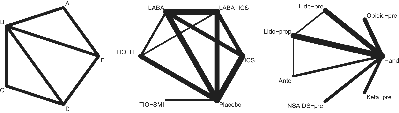
The toy example with five treatments and seven two-arm studies is shown in the left panel of Figure 1. All variances are assumed to be 1. The observed treatment effects for the comparisons A:B, A:E, B:C, B:D, B:E, C:D, and D:E are also assumed to be equal to 1.
Example network graphs. Left panel: A fictitious network with five treatments and seven studies. Middle panel: Network graph of the Dong 2013 data. ICS, inhaled corticosteroid; LABA, long-acting
$\beta 2$
 agonist; TIO-HH, tiotropium dry powder delivered via HandiHaler; TIO-SMI, tiotropium solution delivered via Respimat Soft Mist Inhaler. Right panel: Network graph of the Jalota 2011 data. Ante, Antecubital vein; Hand, Hand vein; Lido-prop, Lidocaine–propofol admixture; Lido-pre, Lidocaine pretreatment; Keta-pre, pretreatment with ketamine; NSAIDS-pre, pretreatment with non-steroidal anti-inflammatory drugs; Opioid-pre, Pretreatment with opioids.

Figure 1 Long description
The figure consists of three panels arranged horizontally.
* Left panel: A pentagonal network graph with nodes labeled A, B, C, D, and E. Node A is at the top. Node B is at the top-left. Node C is at the bottom-left. Node D is at the bottom. Node E is at the right. All nodes are connected by lines of uniform thickness forming a perimeter. Internal connections exist between B and D, and B and E.
* Middle panel: A network graph with six nodes. L A B A is at the top-left, L A B A-I C S is at the top-right, I C S is at the far right, Placebo is at the bottom, T I O-S M I is at the bottom-left, and T I O-H H is at the far left. The thickest lines connect Placebo to L A B A, L A B A-I C S, and T I O-H H. Thinner lines connect L A B A to L A B A-I C S, T I O-H H, and I C S. A very thin line connects T I O-S M I to Placebo.
* Right panel: A network graph with seven nodes arranged in a semi-circle around a central node on the right labeled Hand. Moving clockwise from the top-left, the nodes are Lido-pre, Opioid-pre, Hand (the central hub), Keta-pre, N S A I D S-pre, Ante, and Lido-prop. The thickest lines connect Hand to Lido-prop and Lido-pre. Moderate thickness lines connect Hand to Opioid-pre, Keta-pre, N S A I D S-pre, and Ante. A thin line connects Lido-prop to Lido-pre and Ante.
2.2. Example 2
The second example is an NMA of 41 trials (including seven four-arm studies and three three-arm studies, making 82 pairwise comparisons in total) investigating the safety of six inhaled medications, including placebo, in patients with chronic obstructive pulmonary disease. The outcome was mortality, measured as binary, with the odds ratio as the effect measure.Reference Dong, Lin, Shau, Wu, Chang and Lai 5 The data set is available from the R packages netmeta and metabook.Reference Rücker, Krahn and König 4 , Reference Schwarzer 6 The network graph is shown in the middle panel of Figure 1.
2.3. Example 3
The third example, shown in the right panel of Figure 1, is a network of 102 trials (including three three-arm trials) comparing seven drug and non-drug interventions to prevent pain on propofol injection, with hand vein as reference.Reference Jalota, Kalira and George 7 The binary outcome was pain, with relative risk (RR) as a measure of effect. The data set is available from the R package metabook.Reference Schwarzer 6
3. Methods
Let us assume a connected network and let
$\mathbf {X}$
 be the design matrix of an NMA where the rows represent studies or comparisons (maybe aggregated over studies) and the columns belong to n treatments, represented as nodes in the network graph. Each row of
$\mathbf {X}$
 contains
$1$
 in the column corresponding to one of the treatments in that study (or comparison),
$-1$
 in the column corresponding to the other treatment, and zeros elsewhere. Let
$\mathbf {W}$
 be the diagonal matrix of weights, after adjusting weights for multi-arm trials, where necessary.Reference Rücker
8
For the common-effects model, we use inverse variance weights, and for a random-effects model, we choose an appropriate weight matrix based on one of the proposed estimators for the heterogeneity variance.Reference Veroniki, Jackson and Bender
9
,
Reference Langan, Higgins and Jackson
10
Comparisons for which no study provides information can (but need not) be represented in
$\mathbf {W}$
 with weight zero. The dimension of
$\mathbf {W}$
 must agree with the number of rows in
$\mathbf {X}$
 .
Example 1
For our toy example, the weight matrix is equal to
$\mathbf {W} = \mathbf {I}$
 , the
$7 \times 7$
 identity matrix, and the design matrix is

where the columns correspond to the five treatments (nodes) A, B, C, D, and E and the rows to the seven comparisons listed in Section 2.1 and shown in Figure 1, left panel. Alternatively, we may use the full design matrix, including the non-existent edges AC, AD, and CE and for
$\mathbf {W}$
 the
$10 \times 10$
 identity matrix with zeros at the diagonal positions of the non-existent edges. For real data, the study-based design matrix will be used, such that the rows correspond to studies and studies that compare the same treatments contribute identical rows.
We model the treatment effects in a contrast-based way. Let Y denote the vector of true treatment contrasts. The NMA model is

with a parameter vector
$\beta $
 of length n, weight matrix
$\mathbf {W,}$
 and
$\mbox {Var}(Y | \mathbf {X}) = \mathbf {W}^{-1}$
 . Based on this model,
$\beta $
 is estimated by

where
$\mathbf {L} = \mathbf {X} ^\top \mathbf {W} \mathbf {X}$
 is the Laplacian matrix and
$^+$
 denotes the Moore–Penrose pseudoinverse. We point out that, in the absence of a baseline treatment,
$\hat \beta $
 is only determined up to an additive constant that cancels for
$\mathbf {X} \hat \beta $
 .Reference Rücker and Schwarzer
2
,
Reference Rücker
8
,
Reference Albert
11
.
We now describe two matrices, the covariance matrix and the hat matrix of an NMA. The covariance matrix of the NMA-based treatment effect estimates is obtained as

and the hat matrix
$\mathbf {H}$
 can be written as

$\mathbf {H}$
 and
$\mathbf {C}$
 are quadratic matrices of the same dimension as
$\mathbf {W}$
 . If
$\mathbf {W} = \mathbf {I}$
 , the identity, we have
$\mathbf {H} = \mathbf {C}$
 . Consistent contrasts are estimated by

The hat matrix is a projection matrix that maps the vector
$\mathbf {y}$
 of the observed pairwise contrasts from the studies (i.e., the data) to their consistent NMA counterparts,
$\hat {\mathbf {y}}$
 . The length of
$\mathbf {y}$
 (which is the same as that of
$\hat {\mathbf {y}}$
 ) determines the number of rows in the design matrix
$\mathbf {X}$
 .
Each diagonal element of
$\mathbf {L}$
 corresponds to a treatment (node) in the network and is equal to the sum of the weights in the edges connected to that node, known as the weighted degree of the node. Therefore, we use the diagonal of
$\mathbf {L}$
 to define a vector
$\mathbf {d} = \mbox {diag}(\mathbf {L})$
 , and a diagonal matrix
$\mathbf {D}$
 of weighted degrees. The diagonal elements of
$\mathbf {D}$
 are equal to
$\mathbf {d}$
 and the off-diagonal elements are equal to 0. The weighted adjacency matrix of the network is then given by

For the unweighted case (
$\mathbf {W} = \mathbf {I}$
 ),
$\mathbf {A}$
 is the usual adjacency matrix.
Now we define a transition matrix, also called a diffusion matrix, by

This matrix describes a random diffusion process on the network. The concept of diffusion, related to that of random walks, plays a role in graph theory and its applications, particularly physics, see SpielmanReference Spielman, Naumann and Schenk
12
and Subsection 10.1 in SpielmanReference Spielman
13
, and we applied it to NMA in an earlier paper.Reference Davies, Papakonstantinou, Nikolakopoulou, Rücker and Galla
14
Consider a random walker moving between nodes of the network; each element
$\mathbf {T}_{ij}$
 of the diffusion matrix describes the probability of a walker who is currently at node j, transitioning to node i in the next step. According to Equation (1), this transition probability is proportional to the weight associated with the edge connecting nodes i and j (normalized by the weighted degree of node j). Therefore, the walker is more likely to move along the edges with a larger weight. The movement of the walker is related to the flow of information in the network and the contribution of edges to the network-based treatment effect estimates for each comparison.
Example 1
For the toy example, we have

The columns of
$\mathbf {T}$
 sum up to 1 and describe for each column (node) a multinomial distribution with probabilities for moving from the given node to each of its neighbors. For an unweighted network, non-zero probabilities within the same column are equal; for a general NMA, they become different. These probabilities provide the basis for the infinite diffusion process we describe in the next section.
3.1. A geometric sequence of diffusion matrices
For the following, we first assume that the network graph contains at least one loop of odd length, in other words, it is non-bipartite. We consider the geometric sequence of the powers of the diffusion matrix,
$(\mathbf {T}^i)_{i = 0, 1, 2, \dots }$
 . Under the assumption that this sequence is converging, its limit is the matrix

where
$\mathbf {1}$
 is the vector of ones of length n and
$\mathbf {d}_0$
 is the standardized vector of degree proportions,
$\mathbf {d}_0 = \mathbf {d}/||\mathbf {d}||,$
 where
$||\mathbf {d}||$
 is the sum of the weighted degrees over all nodes.
$\mathbf {T}^{\infty }$
 has n equal columns that are all equal to
$\mathbf {d}_0$
 (see p. 10.1 in SpielmanReference Spielman
13
).
If
$\mathbf {p} = (p_1, \dots , p_n)$
 is a starting vector of probabilities
$0 \le p_i \le 1, i = 1, \dots , n$
 and
$\sum p_i = 1$
 , we have under the assumption of convergence

justifying the notion of
$\mathbf {T}$
 as a diffusion matrix: starting from any distribution of a constant mass over the nodes, iterating
$\mathbf {T}$
 leads to a stable limit distribution of the mass such that each node obtains a mass proportional to its weighted degree.
Example 1
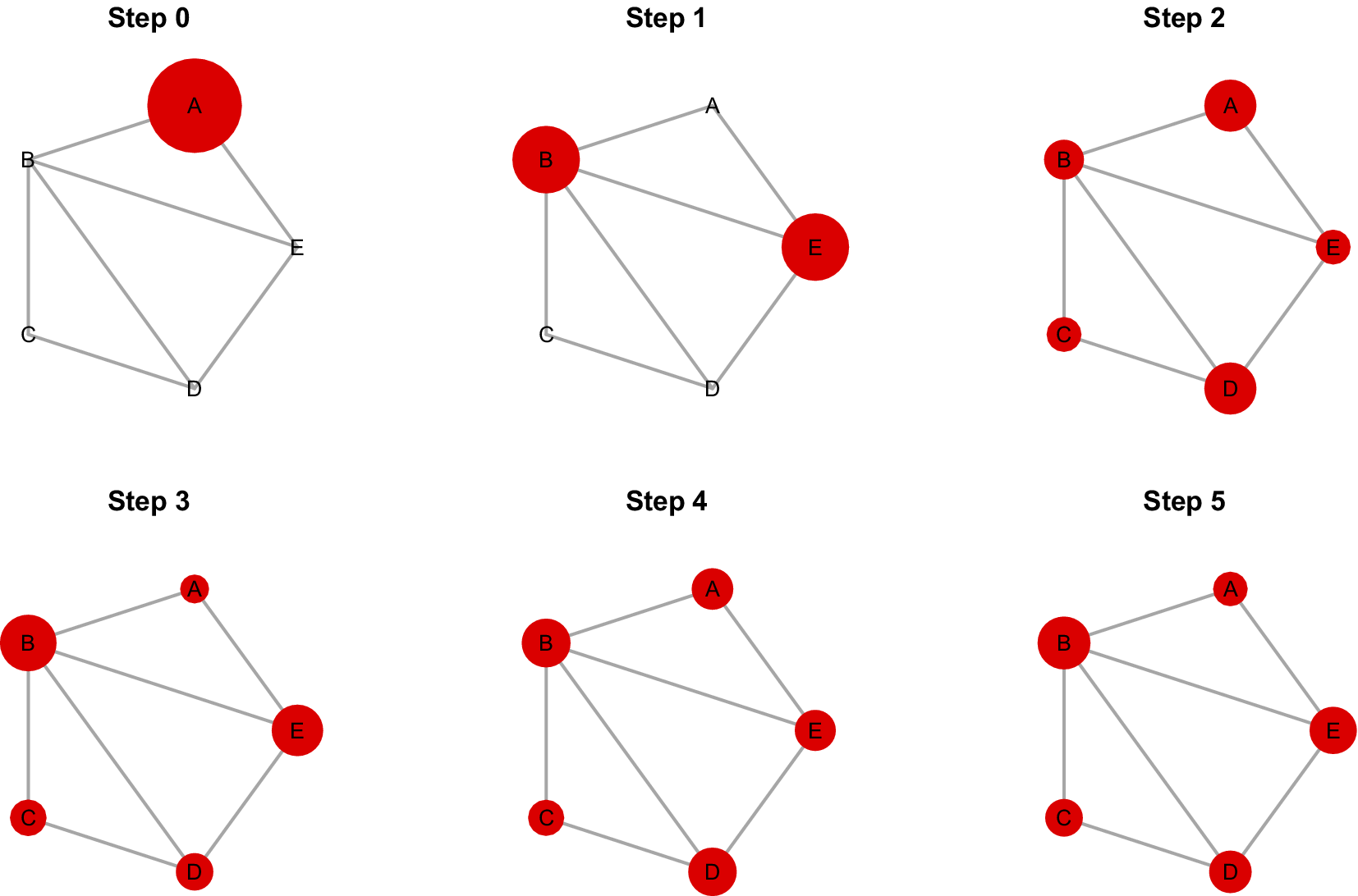
We apply the diffusion process to the toy example (Figure 1, left panel). Figure 2 shows the first six steps of the diffusion process when starting in node A (step 0). In the first step, the mass is equally divided between nodes B and E. In the following steps, the mass is dispersed across all available nodes. The limit distribution is reached with a precision of seven decimal places after 34 steps (see the R script available on Zenodo, as given in the “Data availability statement” section). It is given by

Diffusion process for Example 1, starting in node A.

Figure 2 Long description
The figure consists of six panels labeled Step 0 through Step 5. Each panel shows a pentagonal network of five nodes labeled A, B, C, D, and E connected by gray lines.
* Step 0. Node A is a large red circle. Nodes B, C, D, and E are small black text labels with no red fill.
* Step 1. Node A returns to a small text label. Nodes B and E become large red circles. Nodes C and D remain small text labels.
* Step 2. All nodes except A are red circles. Nodes B and D are medium-sized, while C and E are smaller. Node A is a small red circle.
* Step 3. All five nodes are red circles. Nodes B and E are the largest, followed by D and C, with A being the smallest.
* Step 4. All five nodes remain red circles. The sizes have stabilized with B, D, and E being medium-sized and A and C being slightly smaller.
* Step 5. The network reaches a steady state where all five nodes are red circles of nearly uniform medium size, with B and D appearing slightly larger than A, C, and E.
We note that we did not prove the convergence of the sequence
$(\mathbf {T}^i)_{i = 0, 1, 2, \dots }$
 and the existence of
$\mathbf {T}^\infty $
 . In fact, for bipartite network graphs, this sequence does not converge but oscillates. We will treat this case in Section 3.2.
3.2. Bipartite networks
A bipartite graph is a graph that does not contain odd-numbered loops (cycles). As a result, the nodes can be split into two sets such that nodes from each set are exclusively connected to nodes from the other set and vice versa. Examples are networks without any loops, also called trees, such as star-shaped networks or networks containing only even-numbered loops, all of which occur frequently in NMA.
For bipartite networks, the geometric sequence of diffusion matrices, as defined above, does not converge. Instead, the diffusion matrices oscillate between the two sets of nodes and thus do not lead to a stable limit distribution. Oscillation is a well-known feature of bipartite graphs.Reference Bonchev and Kier 15 , Reference Rücker and Rücker 16 Fortunately, there is a pragmatic solution: We can define a so-called lazy walk, which means that in each step half of the mass remains in the current node and the other half continues to diffuse according to the edge weights. Following Spielman,Reference Spielman, Naumann and Schenk 12 , Reference Spielman 13 the transition matrix is then

(see p. 10.1 in SpielmanReference Spielman
13
), and the limit of the sequence
$\tilde {\mathbf {T}}^i$
 again becomes

As this is the more general version of diffusion, we use a lazy walk in most of the R functions described in Section E. By contrast to the lazy walk, we refer to the walk defined by
$\mathbf {T}$
 in Equation (1) as the simple walk.
3.3. A geometric series of diffusion matrices
If the sequence
$\tilde {\mathbf {T}}^i \rightarrow \mathbf {T}^{\infty } \ne \mathbf {0}$
 converges, the geometric series of the partial sums
$\sum _{i=0}^{N} \tilde {\mathbf {T}}^i \ (i = 0, 1, 2, \dots , N)$
 diverges. However, we can state the following theorem.
Theorem
For both bipartite and non-bipartite networks, the covariance matrix can be written using a geometric series of diffusion matrices:

Corollary
For the hat matrix, we have

This follows immediately from (3).
We note that although the sum of diffusion matrices
$\sum _{i=0}^{\infty } \tilde {\mathbf {T}}^i$
 diverges, Equations (3) and (4) first evaluate the column differences (via multiplication by
$\mathbf {X}^\top $
 ), which causes the sum to converge.
Remark
Equation (3) can also be written using
$\mathbf {T}^\infty $
 :

In contrast to
$\sum _{i=0}^{\infty } \mathbf {T}^i$
 and
$\sum _{i=0}^{\infty } \tilde {\mathbf {T}}^i,$
 the geometric series
$\sum _{i=0}^{\infty } \left (\tilde {\mathbf {T}} - \mathbf {T}^\infty \right )^i$
 is convergent; for details, see Appendix C.
Alternative: Diffusion with an absorbing node
As an alternative to the unlimited walk as described above, we can choose any treatment as the baseline, which means reducing the design matrix
$\mathbf {X}$
 by the respective column, giving
$\mathbf {X}_r$
 , and reducing the other matrices by the respective column and row, giving
$\mathbf {D}_r$
 and
$\mathbf {T}_r$
 with dimension
$n-1$
 . We call node r the reference node. As described in Appendix B, the reference node becomes absorbing, which means that all walks eventually end up there, and the geometric series
$\sum _{k=0}^\infty \mathbf {T}_r^k$
 becomes convergent. We then have

which holds in general, also for bipartite graphs.
Using a simplified version of the proof in Appendix A, it is possible to show that, for the special case of a non-bipartite graph, the covariance and hat matrices can also be found by replacing the reduced matrices
$\mathbf {X}_r$
 ,
$\mathbf {D}_r$
 , and
$\mathbf {T}_r$
 in Equation (6) with their unreduced counterparts.
3.3.1. Finding NMA estimates iteratively
Equations (3)–(6) mean that we can obtain the covariance matrix
$\mathbf {C}$
 and the hat matrix
$\mathbf {H}$
 iteratively, without computing an inverse or pseudoinverse matrix. Given a vector of observed relative treatment effects
$\mathbf {y}$
 , we can estimate the true effects by the consistent solution
$\hat {\mathbf {y}},$
 where

This suggests approximating
$\hat {\mathbf {y}}$
 by a series of vectors

which perform the sum up to some finite value N. The goodness of the approximation can be measured by the weighted sum of squared differences

starting with
$Q = (\mathbf {y} - \hat {\mathbf {y}})^\top \mathbf {W} (\mathbf {y} - \hat {\mathbf {y}})$
 . The examples (see the R script) often show a remarkably good approximation already in the first iteration steps. To understand why, we look at the very first step,
$N=0$
 . For
$N=0$
 , we have
$\tilde {\mathbf {T}}^0 = \mathbf {I}$
 and

Due to the structure of
$\mathbf {X}$
 , in this first step, the observations
$\mathbf {y}$
 are mapped onto a set of
$n-1$
 consistent relative effects,
$\hat {\mathbf {y}}_0$
 (see Section 3.1.2 in Rücker and SchwarzerReference Rücker and Schwarzer
2
). Particularly, entries of
$\mathbf {y}$
 from different studies that represent the same comparison are mapped to the same value in
$\hat {\mathbf {y}}_0$
 . As N increases, these consistent effects move closer to the set of effects that minimize the weighted sum of squared differences.
4. Interpretation
For any transition matrix
$\mathbf {T}$
 (also
$\tilde {\mathbf {T}}, \mathbf {T}_r$
 ), each element (e.g.,
$\mathbf {T}_{ij}$
 ) describes the probability of a transition from node j to node i. Element
$(i,j)$
 of
$\mathbf {T}^2$
 is given by

which describes the probability of arriving at node i after two steps when starting in node j. An analogous interpretation holds for
$\mathbf {T}^3_{ij}, \mathbf {T}^4_{ij}, \dots $
 and so on.
4.1. Illustration 1: Length of stay
Consider a walker who starts in node A (step 0), switches to node B in step 1, then comes back to node A in step 2, and leaves A again in step 3. Until now, this walker has spent a total of two steps in node A. Now consider many such walkers on the network, who have a probability
$p_i$
 of starting in node i. The expected total time a walker spends in node i after N steps is calculated by counting the number of walkers in node i at step k, then summing these counts up to a total number of steps N, and dividing the result by the total number of walkers. Therefore, the vector of expected times spent in each node is given by

where
$\mathbf {p} = (p_1, \dots , p_n)^\top $
 is the starting distribution of the walk. For example, setting
$\mathbf {p}$
 equal to the first unit vector gives the first column of
$\sum _{k=0}^N\mathbf {T}^k$
 , which contains the expected length of stay in each node up to step N for those who start their walk in node
$1$
 . The larger N becomes, the less this time depends on the starting point. However, unlike the stationary distribution of the walk in Equation (2), which describes the fraction of time spent in each node (and converges to the weighted degree of the node for large N), the total time until step N retains the dependence on the starting point. We also note that, because we are dealing with discrete time, the expected time spent in a node is the same as the expected number of visits to that node.
4.2. Illustration 2: Walkers and drinks
To provide a perhaps more comprehensible interpretation of times, we now mark the network nodes, for example, by placing colored flags, such as yellow, orange, red, green, and so on. Large numbers of walkers, wearing T-shirts in the same colors, are placed at “their own” node. There are also n drinks in various colors available, such as lemon juice, orange juice, red currant juice, kiwi juice, etc. We place n bottles, each with one of the different drinks, at each node, as shown in Figure 3 for Example 1 (
$n=5$
 ). As before, we are working with discrete time. Before starting their walk, each walker takes a small, standardized sip of “their own” drink at their starting node; for example, “yellow” walkers take a sip of lemon juice. Then, all walkers simultaneously start stepwise dispersing through the network, taking each branch with probability proportional to its weight and taking a standardized sip of “their own” drink at every station they reach. At any time, all walkers have had the same juice intake. However, nodes with a larger (weighted) degree have been visited by more walkers, and the bottles at those nodes contain less juice.
A network with five colored nodes and corresponding drinks. Walkers are spreading through the network in steps, taking a sip of their own drink at every station they visit.

4.2.1. Scaling—Reducing by degree
After a large number of N steps, the remaining juice in each bottle is now further reduced according to the node’s (weighted) degree. For example, if the degree is 2, half of every bottle is poured away; if the degree is 3, two-thirds of each bottle are removed. This action, which we call scaling, corresponds to multiplying the geometric series
$\sum _{k=0}^N\mathbf {T}^k$
 by
$\mathbf {D}^{-1}$
 on the left.
4.2.2. Column differences
Multiplication with
$\mathbf {X}^\top $
 on the right means comparing the remaining volume of juice between pairs of bottles of different colors at the same node, for each node in the network. These differences are only due to the different starting positions of the walkers.
4.2.3. Row differences
Multiplication with
$\mathbf {X}$
 on the left means comparing the differences above between nodes. The resulting “differences of differences” in volume then correspond to the covariances in NMA (see below). We note that, because we are calculating differences of differences, it is not necessary that the size of bottles at the beginning is equal for each node. The only requirement is that all bottles must start with enough liquid to facilitate the total number of walkers removing liquid over N steps.
The walkers-and-drinks model suggests an interpretation of the NMA covariance matrix in terms of the long random walk. We measure the difference between the amount of A-juice and B-juice, remaining at A, and the difference between the amount of A-juice and B-juice, remaining at B. We write the difference of differences as

where we have used the fact that, due to symmetry,
$A_B = B_A$
 (see Appendix D). This may be interpreted as the difference between the fluid intake “at home” (i.e., A in A and B in B) and intake “at one’s neighbor’s” (A in B or B in A). We have implemented the diffusion process in a number of R functions described in Appendix E.
5. Results
5.1. Example 1
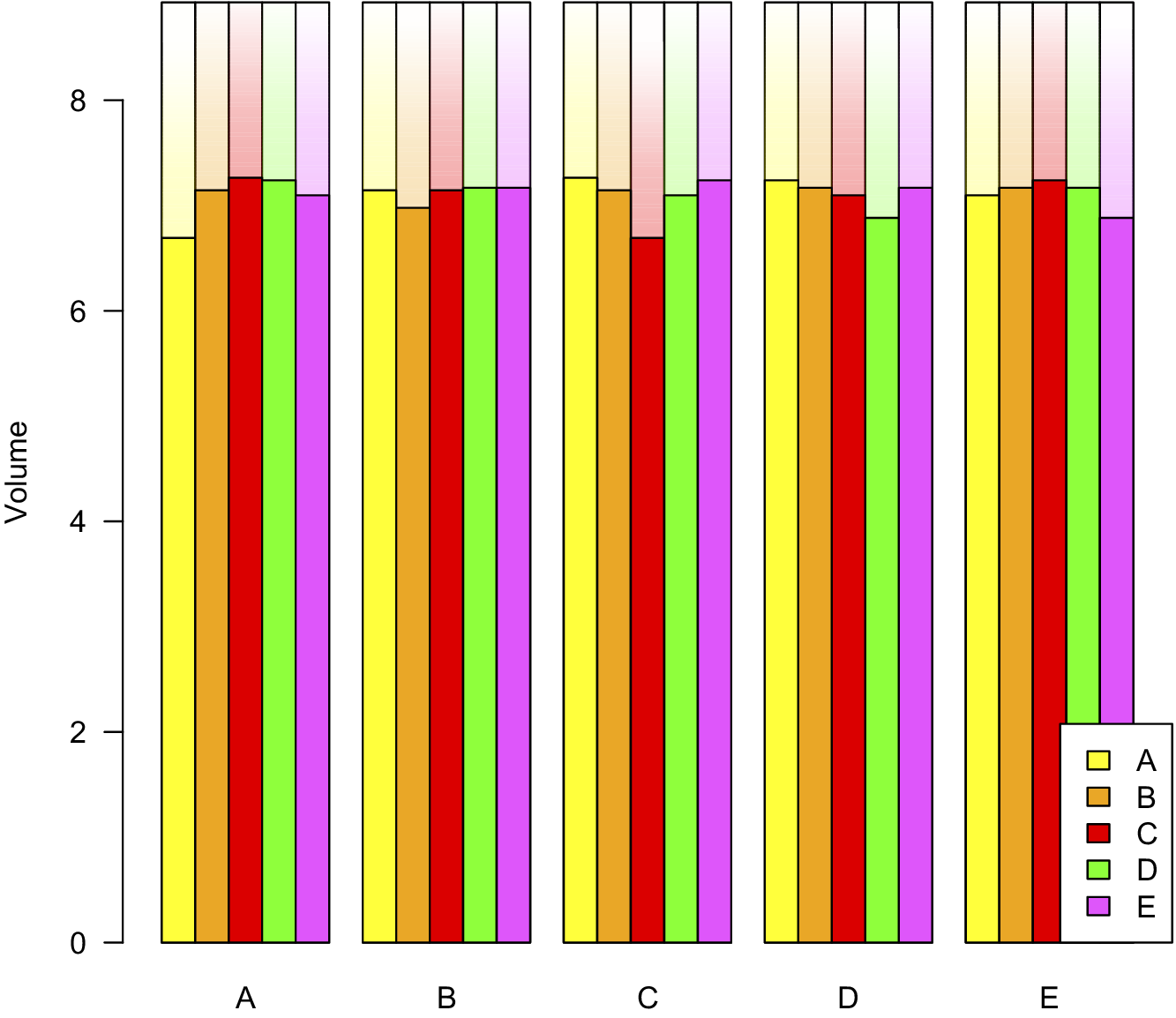
We have shown the diffusion process for the toy example already in Section 3.1 (Figure 2). Figure 4 illustrates the walkers-and-drinks interpretation. The bars represent the remaining juice in the bottles after 50 walking steps and pouring away part of the juice according to the node’s degree. The differences of differences between the nodes correspond to the covariances in NMA. For example, the yellow and the red bar in B have the same height, 7.14, but in A the red bar is higher, 7.26, than the yellow bar, 6.69, with a difference of 0.57. This is the covariance matrix entry for (A:B, A:C).
Walkers-and-drinks model for Example 1. The bars represent bottles with juice left after 50 steps and scaling. Each block of bars belongs to a node, each bar in a particular color belongs to the walkers from a particular node. Yellow = A, orange = B, red = C, green = D, and violet = E.

Figure 4 Long description
The Y-axis is labeled Volume and ranges from 0 to 8. The X-axis contains five categorical labels: A, B, C, D, and E. Each label corresponds to a cluster of five vertical bars.
Each bar in a cluster is color-coded: yellow for A, orange for B, red for C, green for D, and violet for E. The bars are partially filled with solid color at the bottom and fade to white at the top, with a horizontal line indicating the specific volume level.
* Cluster A: Yellow is at approximately 6.7, orange at 7.1, red at 7.3, green at 7.2, and violet at 7.1.
* Cluster B: Yellow is at 7.1, orange at 7.0, red at 7.1, green at 7.2, and violet at 7.2.
* Cluster C: Yellow is at 7.3, orange at 7.1, red at 6.7, green at 7.1, and violet at 7.2.
* Cluster D: Yellow is at 7.2, orange at 7.1, red at 7.1, green at 6.9, and violet at 7.2.
* Cluster E: Yellow is at 7.1, orange at 7.2, red at 7.3, green at 7.2, and violet at 6.9.
A legend in the bottom right corner maps the colors to letters A through E.
5.2. Example 2
Figure 5 shows how the estimated treatment effects of the second example (41 studies with 82 direct comparisons) evolve with each iteration of the geometric series that approximates the hat matrix, here using the lazy walk method. For the comparisons with direct evidence, the treatment effects converge quickly from their direct estimates to their network estimates (note that two pairs of estimates are very similar and cannot be easily distinguished in the figure). As noted in Section 3.3.1, the 82 direct observations are mapped to only 10 consistent estimates already in iteration step 0.
Iterative estimation of the treatment effects for Example 2. The starting points of the lines (to the left of step 0) are the observed treatment effects from 82 comparisons. Each number at the bottom represents the weighted sum of squared distances of the estimates from the final NMA estimates.

Figure 5 Long description
A line graph with the Y axis labeled Treatment effect ranging from negative 0.6 to 0.4 and the X axis labeled Iteration step ranging from 0 to 10.
* Data Flow: On the far left, before step 0, dozens of multicolored lines are widely scattered across the entire Y axis range. As they move toward step 0, they converge sharply. Between steps 0 and 4, the lines stabilize into approximately 10 distinct horizontal paths. By step 10, these lines are nearly flat, representing final N M A estimates.
* Bottom Values: A series of numbers representing weighted sum of squared distances is printed just above the X axis. From left to right, these values are: 41.14, 3.43, 0.92, 0.29, 0.1, 0.04, 0.01, 0.01, 0, 0, 0, 0.
* Trends: The values at the bottom decrease rapidly as the iteration steps increase, corresponding to the visual stabilization and convergence of the treatment effect lines.
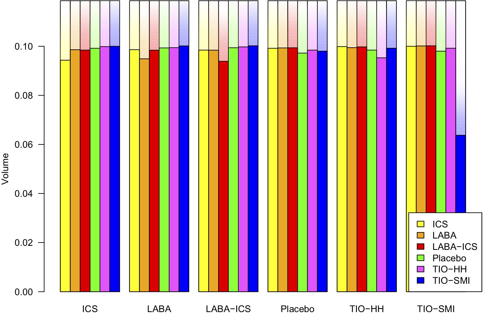
Figure 6 illustrates the walkers-and-drinks interpretation for this data. The most noticeable feature of this graph is the short blue bar at its corresponding node, TIO-SMI. As we see from the network graph (Figure 1, middle panel), this node is a spur, connected only to placebo and weakly, via only two trials. The height difference between the blue bar (TIO-SMI) and every other is small at all other nodes but is large at node TIO-SMI. This causes the difference in differences to be particularly large for all comparisons involving TIO-SMI. This makes sense as, by Equation (3), these differences in differences equal the variances of these comparisons, which will be large because they rely heavily on the two studies comparing TIO-SMI and placebo.
Walkers-and-drinks model for Example 2. The bars represent bottles with juice left after 50 steps and scaling. Each block of bars belongs to a node, each bar in a particular color belongs to the walkers from a particular node. Yellow = ICS, orange = LABA, red = LABA-ICS, green = Placebo, violet = TIO-HH, and blue = TIO-SMI.

Figure 6 Long description
The y-axis is labeled Volume and ranges from 0.00 to 0.10. The x-axis contains six categorical groups labeled from left to right: I C S, L A B A, L A B A-I C S, Placebo, T I O-H H, and T I O-S M I. Each group contains a cluster of six vertical bars. The bars are color-coded as follows: yellow for I C S, orange for L A B A, red for L A B A-I C S, green for Placebo, violet for T I O-H H, and blue for T I O-S M I.
Across the first five groups (I C S through T I O-H H), the volume levels for all bars are relatively uniform, hovering near the 0.10 mark with minor fluctuations. However, in the final group on the far right, T I O-S M I, there is a significant drop in the blue bar, which represents the T I O-S M I node, falling to approximately 0.06. The other five bars in this final group remain near 0.10. Each bar is topped with a semi-transparent faded extension reaching the top of the frame.
5.3. Example 3
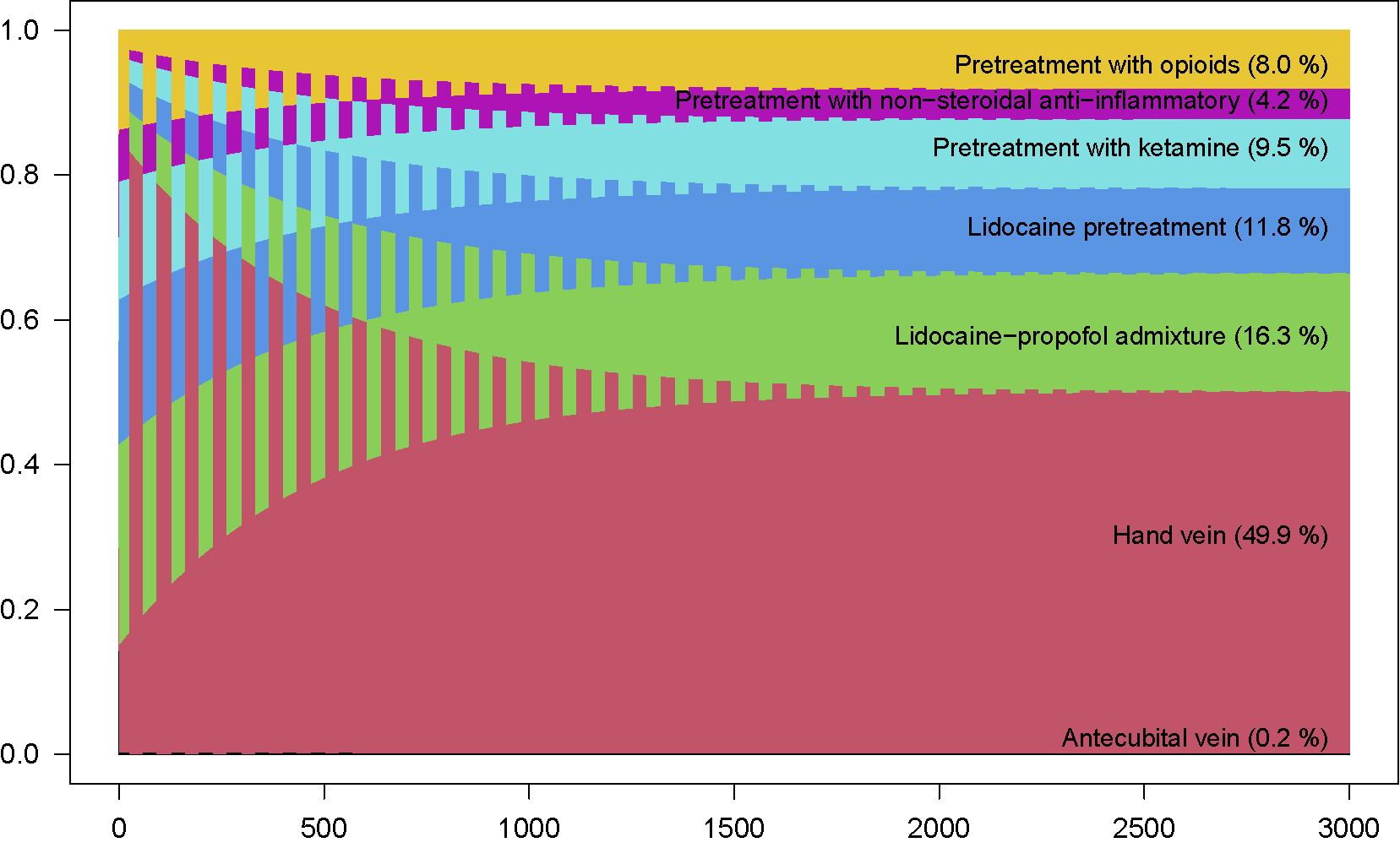
As Figure 1 (right panel) shows, the network graph is almost star-shaped, with weak connections between treatments Ante and Lido-prop (one three-arm study) and between Lido-pre and Lido-prop (two three-arm studies). This graph is not bipartite, but could be seen as “almost bipartite,” as demonstrated by Figure 7, which shows 3,000 steps of simple diffusion in the form of a stacked probability plot, starting with equal mass at each node and ending with the proportional weighted degrees. We see oscillatory behavior for about 2,000 steps.
Simple diffusion for Example 3, starting with uniform distribution. The numbers are the percentage weighted degrees.

Figure 7 Long description
The x-axis ranges from 0 to 3000 and the y-axis ranges from 0.0 to 1.0. At the start on the left, the areas are vertically striped and overlapping, representing a uniform distribution. As the x-axis progresses, the areas smooth into solid horizontal bands, reaching a steady state by approximately 1500.
From bottom to top, the final distribution layers are:
* Antecubital vein at 0.2 percent, a thin black line at the base.
* Hand vein at 49.9 percent, a large red section.
* Lidocaine-propofol admixture at 16.3 percent, a green section.
* Lidocaine pretreatment at 11.8 percent, a blue section.
* Pretreatment with ketamine at 9.5 percent, a light blue section.
* Pretreatment with N S A I D S at 4.2 percent, a purple section.
* Pretreatment with opioids at 8.0 percent, a yellow section at the top.
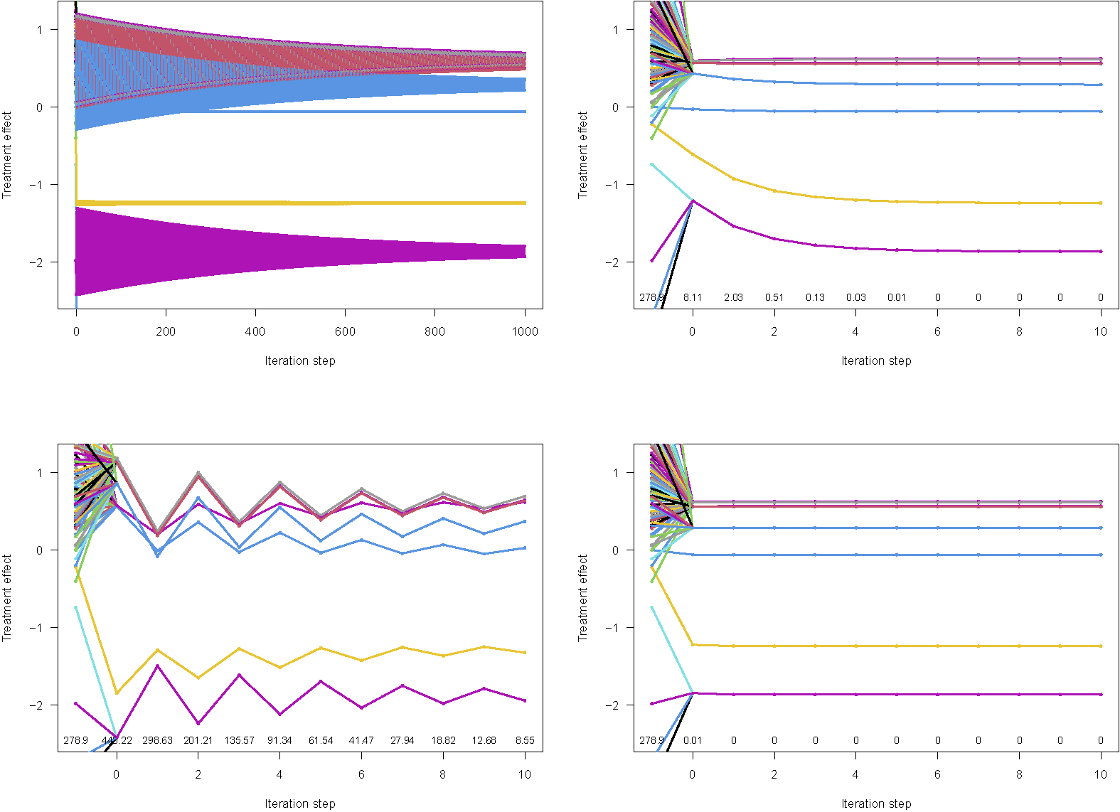
Iterative estimation of the treatment effects for Example 3. The starting points of the lines are the observed treatment effects from 108 comparisons. Top left: Simple method, 1,000 steps; Top right: Lazy walk, 10 steps. Bottom left: Absorbing walk, reference is Lidocaine–propofol admixture, 10 steps. Bottom right: Absorbing walk, reference is Hand vein, 10 steps. Each number at the bottom represents the weighted sum of squared distances of the estimates from the final NMA estimates.

Figure 8 Long description
A four-panel set of line graphs. Each graph shares the same Y-axis labeled Treatment effect ranging from minus 2 to 1 and an X-axis labeled Iteration step.
* Top-left panel: Simple method. The X-axis ranges from 0 to 1,000. Numerous colored lines originate at step 0 and gradually converge toward specific horizontal values as they move toward step 1,000. One group converges near 0.5, another near 0.2, and a third near minus 1.8.
* Top-right panel: Lazy walk with 10 steps. The X-axis ranges from 0 to 10. Lines show rapid convergence within the first 4 steps. A row of numbers at the bottom indicates the weighted sum of squared distances, starting at 278.9 and reaching 0 by step 6.
* Bottom-left panel: Absorbing walk with Lidocaine-propofol admixture as reference. The X-axis ranges from 0 to 10. The lines exhibit a jagged, oscillating pattern that slowly dampens but does not reach a flat horizontal state by step 10. The bottom numbers decrease from 278.9 to 33.86.
* Bottom-right panel: Absorbing walk with Hand vein as reference. The X-axis ranges from 0 to 10. Lines show immediate convergence to horizontal paths by step 1. The bottom numbers drop from 278.9 to 0.01 at step 0 and remain at 0 for all subsequent steps.
Figure 8 shows four versions of the iteration for the relative treatment effect estimates. In Figure 8 (top left), we see that the simple walk (Equation (1)) oscillates very strongly, it needs about 3,000 steps to converge (see also Figure 7). By contrast, the lazy walk (Equation (4), top right) converges after only 10 steps. The bottom plots show the convergence of absorbing walks (Equation (6)) with two different reference treatments. The bottom left plot shows oscillatory behavior for the first 10 steps of the absorbing walk with reference treatment Lidocaine–propofol admixture. The bottom right plot shows fast convergence for the absorbing walk with reference treatment Hand vein. This example shows that oscillation may also occur for non-bipartite graphs and demonstrates that absorbing walks tend to converge most quickly if a central node (i.e., a node with maximum weighted degree) is chosen as reference.
6. Discussion
In this article, we have shown that the covariance matrix of the network estimates in an NMA can be written as a geometric series of diffusion matrices, framed by the design matrix and its transpose. A similar representation exists for the hat matrix.
This work was partly motivated by a method called network deconvolution that was introduced in the causal inference literature.Reference Feizi, Marbach, Médard and Kellis 17 , Reference Lin, Pan and Pan 18 These authors assume that similarities between variables, or even directed causal effects, can be described by some matrix, such as a correlation matrix. The powers of this matrix, suitably scaled, are summed up to provide a matrix of “total effects” called the “transitive closure” that can be observed. This process is also known as network convolution. The inverse process of identifying the starting matrix, given its transitive closure, is called network deconvolution. In our context of NMA, this would correspond to finding the diffusion matrix from a given covariance matrix, which would be a different task. Apart from that, it seems questionable whether multiplying correlation matrices makes sense, given that correlation is not transitive.
Matrix power series have many applications, for example, in physics (random walks on electrical networksReference Doyle and Snell 19 ), chemistry (symmetry recognition in chemical compoundsReference Rücker and Rücker 20 ), or biology (Krylov subspacesReference Frost 21 , Reference Frost 22 ). A geometric series of matrices is also called a Neumann series.Reference Werner 23 Finite Neumann series are used in applications to approximate the inverse of a matrix by iteration; for an example, see Wu et al.Reference Wu, Yin, Vosoughi, Studer, Cavallaro and Dick 24
The iterative calculation of the covariance matrix naturally allows a similar iteration for the hat matrix and thus an iterative method for finding the network estimates that, in most of our examples, is fast converging. For the version with an absorbing node, the speed of convergence depends on the choice of the reference node. We experienced the best convergence when choosing a central node (e.g., placebo as a frequently used control treatment, or hand vein for Example 3). This is plausible, as a central node rapidly absorbs all the mass. Thus, the reduced transition matrix, described in Appendix B, converges quickly to the null matrix, causing the geometric series to reach its limit.
Example 3 demonstrates that for nearly star-shaped networks, with a distinguished central node, the version with the central node chosen as absorbing is clearly superior. Although the algorithm tends to be slow for complex networks, it seems generally to be numerically stable. Of note, even complex treatment networks are relatively small compared to large graphs in other application areas.
More generally, the speed of convergence is driven by the features of the network on the one hand and the chosen diffusion method on the other hand. Network features are the density of the network and its extent of “bipartiteness” (leading to oscillation, except for the lazy walk method). Density (or the degree of connectedness) can be measured, for example, by the second-smallest eigenvalue of the Laplacian matrix, also called the Fiedler value (which needs to be standardized for weighted networks). Similarly, bipartiteness can be measured by the magnitude of the smallest eigenvalue of the lazy diffusion matrix (if it equals 0, the graph is bipartite; see Subsection 1.5.4 in SpielmanReference Spielman 13 ). With respect to the method, the method with an absorbing node seems generally preferable, provided that a central node (ideally the one with maximum weighted degree) is chosen as the absorbing node.
At the comparison-aggregated level,
$\mathbf {H}_{AB,AB}$
 represents the proportion of direct evidence from edge AB for comparison A:B.Reference Dias, Welton, Caldwell and Ades
25
–
Reference Rücker, Papakonstantinou, Nikolakopoulou, Schwarzer, Galla and Davies
28
With study-level input, the individual diagonal elements represent study-specific leverages; their sum over all study contrasts corresponding to edge AB gives the corresponding edge-level quantity.Reference Rücker and Schwarzer
2
,
Reference König, Krahn and Binder
26
,
Reference Rücker, Nikolakopoulou, Papakonstantinou, Salanti, Riley and Schwarzer
29
Another interpretation of the hat matrix comes from the area of electrical circuits. Davies et al. showed that entry
$\mathbf {H}_{AB,CD}$
 can be interpreted as the current flowing through edge CD when a battery is attached across A and B.Reference Davies, Papakonstantinou, Nikolakopoulou, Rücker and Galla
14
Based on an analogy between electrical networks and random walks, this is equal to the expected net number of times a walker who starts a random walk from node A crosses the edge CD before eventually arriving at node B. Our illustration with times adds another interpretation: If we choose a reference node, say B, this node becomes absorbing, all walks eventually end in B, and the expected times in all other nodes become finite (see Appendix B). It turns out that
$\mathbf {H}_{AB,CD}$
 corresponds to the scaled difference in the expected total length of stay in A between walkers who start in C and those who start in D, all walkers eventually arriving in B.
In fact, our work highlights the potential for even further connections between NMA and the study of complex networks in other disciplines. For example, the effective resistance of a graph takes the same form as the variance in NMA.Reference Rücker 8 In the random walk literature, there is an established interpretation for effective resistance in terms of “escape probability,” that is, the probability that a walker who starts in node A, reaches node B before they return to A.Reference Doyle and Snell 19 More recently, Estrada interpreted effective resistance as a diffusion distance.Reference Estrada 30 By defining a diffusion process on a graph, he shows that the effective resistance between two nodes is equivalent to a difference in mass concentrations between the nodes, relative to their initial conditions. This result is closely connected with our own and warrants further investigation.
Bipartite networks, which occur frequently in NMA, have a special structure that must be taken into account. A bipartite network graph must not be confused with a different application of bipartite graphs that occurs when an NMA is represented as a hypergraph, as suggested recently.Reference Lumley 31 , Reference Davies 32 A hypergraph is a generalized graph, where generalized “hyperedges” (in the context of NMA, studies) can join more than two vertices (here treatments, thus including multiarm studies). Each NMA hypergraph can be interpreted as a bipartite graph that consists of two sets of vertices, one representing the treatments, the other representing the studies; both sets are joined by edges where a treatment was investigated in a study.
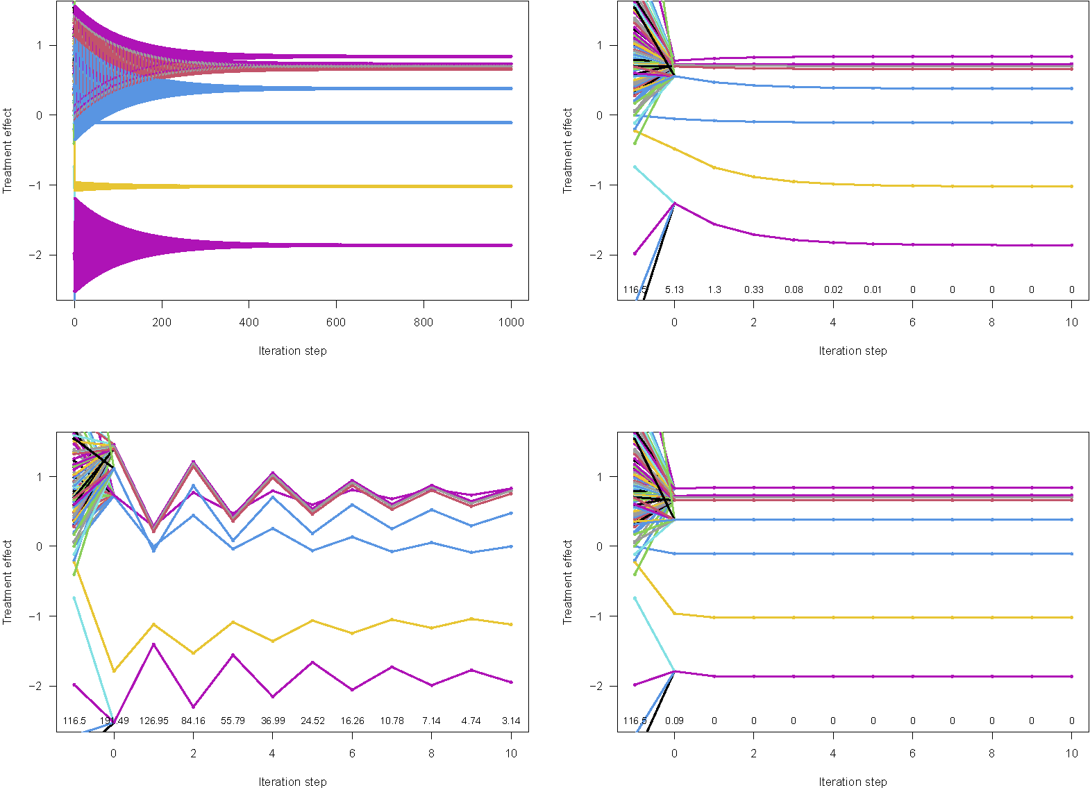
In the present article, we concentrated on the common-effects model. As mentioned, all considerations can be extended to the random-effects model by choosing an appropriate weight matrix. We note, however, that this does not address uncertainty in the estimation of the random-effects heterogeneity variance. As an example, we provide the analog to Figure 8 for the random-effects model in Appendix F.
We are aware that the phenomena described in this article, interesting though they may be, have no direct consequences for NMA application practice, as all essential NMA calculations are easily conducted by standard software. Nevertheless, we believe that our findings reveal a nice connection between regression analysis for NMA and the concepts of diffusion and random walks in network analysis, and they may stimulate further theoretical developments. For example, matrix inverses sometimes make theoretical proofs difficult, and being able to express these as geometric series may help with this sort of work.
Author contributions
Conceptualization: G.R.; Data curation: G.R.; Formal analysis: G.R.; Methodology: G.R., A.L.D.; Project administration: G.R.; Software: G.R., G.S.; Visualization: G.R., G.S.; Writing—original draft: G.R., A.L.D., G.S.; Writing—review and editing: G.R., A.L.D., G.S.
Competing interest statement
The authors declare that no competing interests exist.
Data availability statement
The R script and datasets supporting this work are openly available on Zenodo at https://zenodo.org/records/23134102.
Funding statement
A.L.D. is funded by the Engineering and Physical Sciences Research Council (EP/Y007905/1).
Appendix
A. Proof of Theorem (3)
We assume a connected network and positive weighted degrees for all included nodes. Due to
$\mathbf {T} = \mathbf {I} - \mathbf {L} \mathbf {D}^{-1}$
 , we have
$\mathbf {L} \mathbf {D}^{-1} = \mathbf {I} - \mathbf {T}$
 . Further, it holds
$\mathbf {X} = \mathbf {X} \mathbf {L}^+ \mathbf {L}$
 (see Appendix A.2 in Rücker and SchwarzerReference Rücker and Schwarzer
2
). Using these two relations, we start from the right-hand side of (3) by stating that

and continue with evaluating the finite sum on the right-hand side for a large N:

For the limit, we have because of
$\tilde {\mathbf {T}}^N \to \mathbf {T}^\infty $
 and
$\mathbf {T}^\infty \mathbf {X}^\top = \mathbf {0}$
 :

which proves the theorem.
B. Version with reference node
The idea also works, it even simplifies, if we choose an arbitrary baseline treatment, the reference node, and accordingly reduce the design matrix by the column that belongs to the reference node. All other matrices are reduced analogously, which means deleting the row and column that correspond to the reference node. This has interesting consequences. Let us denote the reduced versions by the index r. First, the Laplacian matrix
$\mathbf {L}_r$
 becomes regular, such that
$\mathbf {L}_r^{-1}$
 exists. Second, with respect to diffusion, the reference node becomes absorbing: each walk eventually ends up in this node. This also holds for bipartite networks. For
$k \to \infty ,$
 we have
$\mathbf {T}_r^k \to \mathbf {0}$
 and
$\sum _{k=0}^\infty \mathbf {T}_r^k$
 is a finite matrix. The same holds for the lazy walk diffusion matrix
$\tilde {\mathbf {T}}_r = (\mathbf {T}_r + \mathbf {I}_r)/2$
 . For the covariance matrix, we have

It turns out that for the version with a reference node, bipartite graphs do not need special attention: the results for the walk described by
$\mathbf {T}_r$
 and for the lazy walk
$\tilde {\mathbf {T}}_r$
 agree.
C. The behavior of
$\sum_{i=0}^\infty({\mathbf{T}} - {\mathbf{T}}^\infty)^i $


We show Equation (5). For
$i> 0,$
 we have

which can be shown by complete induction. Because of
$\mathbf {T}^\infty \mathbf {X}^\top = \mathbf {0,}$
 we may write

Although it has been shown for the average length of stay that
$\frac {1}{N} \sum _{i=0}^N \mathbf {T}^i \rightarrow \mathbf {T}^\infty ,$
 Reference Norris
33
the following simple example shows that series
$\sum _{i=0}^N(\mathbf {T} - \mathbf {T}^\infty )^i$
 and
$\sum _{i=0}^N(\tilde {\mathbf {T}} - \mathbf {T}^\infty )^i$
 generally do not approach the null matrix for
$N \to \infty $
 .
Example
We consider a simple triangle with all standard errors equal to 1. Then

Because the spectral radius of matrix
$\mathbf {T}-\mathbf {T}^\infty $
 is less than 1, the matrix
$\mathbf {I} - (\mathbf {T}-\mathbf {T}^\infty )$
 is nonsingular and the corresponding series gives

which is not the null matrix. A similar consideration holds for
$\tilde {\mathbf {T}}$
 .
D. Symmetry
We note that the matrices
$\mathbf {D}^{-1} \sum _{i=0}^{N} \mathbf {T}^i$
 and
$\mathbf {D}^{-1} \sum _{i=0}^{N} \tilde {\mathbf {T}}^i$
 are symmetric. To see this, we need that
$\mathbf {D}^{-1} \mathbf {T}$
 and
$\mathbf {D}^{-1} \tilde {\mathbf {T}}$
 are symmetric:

which follows from the symmetry of
$\mathbf {D}$
 and
$\mathbf {A}$
 . The same holds for the powers of
$\mathbf {T}$
 and
$\tilde {\mathbf {T}}$
 and their sums and the covariance matrix (3).
E. Implementation in R
The supporting information to this article on Zenodo contains three R scripts to reproduce the results (see the “Data availability statement” section). Script functions.R contains a number of functions, data.R provides the data sets, and analysis.R runs the functions on the examples. We note that data.R and analysis.R provide additional data and analyses that are not shown in this article.
Iterative estimation of the treatment effects for Example 3 based on the random-effects model. The starting points of the lines are the observed treatment effects from 108 comparisons. Top left: Simple method, 1,000 steps; Top right: Lazy walk, 10 steps. Bottom left: Absorbing walk, reference is Lidocaine–propofol admixture, 10 steps. Bottom right: Absorbing walk, reference is Hand vein, 10 steps. Each number at the bottom represents the weighted sum of squared distances of the estimates from the final NMA estimates.

Figure E1 Long description
A multi-panel figure with four line graphs. All graphs share a common Y axis labeled Treatment effect ranging from minus 2 to 1 and an X axis labeled Iteration step.
* Top left panel: Simple method. The X axis ranges from 0 to 1,000. A dense cluster of multicolored lines starts at step 0 with high variance and gradually converges into several distinct horizontal bands by step 400, remaining stable through step 1,000.
* Top right panel: Lazy walk. The X axis ranges from 0 to 10. Lines converge rapidly within the first 2 steps. Small numbers at the bottom indicate weighted sum of squared distances decreasing from 278.9 to 0.
* Bottom left panel: Absorbing walk with Lidocaine-propofol admixture reference. The X axis ranges from 0 to 10. The lines exhibit a persistent zigzag or sawtooth pattern, failing to converge to a single horizontal value. Weighted sum values at the bottom decrease slowly from 278.9 to 12.72.
* Bottom right panel: Absorbing walk with Hand vein reference. The X axis ranges from 0 to 10. Lines show immediate convergence to stable horizontal paths by step 1. Weighted sum values drop sharply from 278.9 to 0 by step 1.
-
1. Function Power() calculates matrix powers. Its arguments are a square matrix $\mathbf {M}$
and a natural number k (the power). The value of the function consists of the
$k'$
th power of
$\mathbf {M}$
,
$\mathbf {M}^k$
, and the partial sum
$\sum _{i=0}^k \mathbf {M}^i$
of the geometric series. -
2. Function diffusion() can be used to visualize the exchange of mass between the nodes of a network, given a netmeta object, a starting distribution (i.e., a vector), and a power N. There are two plotting options, guided by a logical argument proportions. The function provides either a series of network graphs (proportions = FALSE, default) showing how the mass distribution over the nodes develops with $i = 1, \dots , N$
, or a colored stacked probability plot to show this in one figure (proportions = TRUE). An argument diffusion.type allows users to choose between a simple walk ("simple", default), the lazy walk ("lazy"), or a walk with an absorbing node ("absorbing"). Argument ref can be used to specify a reference node. -
3. Function Hat() serves to calculate the hat matrix using a matrix power series via Equations (3)–(6). Its arguments are a netmeta object, a power N, and a logical argument ref, FALSE by default. Argument ref can be used to specify a reference node.
-
4. Function draw.TE() is based on Hat(). For a given netmeta object and a power N, it allows visualizing the iterative course from the given vector of treatment effects TE to the network estimates TE.nma.common and produces a series of essentially decreasing Q values. Users can choose between the various diffusion types (argument diffusion.type) and specify a reference node (argument ref).
-
5. Function draw.hat(), likewise based on Hat(), helps visualizing the iterative course of the hat matrix diagonal (argument hat, default is TRUE), or the same for the treatment effect variances. As with function draw.TE(), there is a choice between diffusion types (argument diffusion.type) and a reference node can be specified (argument ref).
-
6. Function walk() calculates the steps described in the walkers-and-drinks model for a given netmeta object and visualizes them as bar charts.






 Open access

