Implications
Lameness in sows is a common welfare and animal health challenge. Management tools to support farmers and stockpersons in lameness detection are beneficial. Positioning data and acceleration measurements of group-housed sows in the gestation unit are tested to detect lameness in sows. Analysis showed that the walked distance of a sow during a day reduced the days before lameness treatment occurred. Acceleration measurements were not affected. However, before practical implementation further improvements are needed.
Introduction
Sow lameness is a welfare and animal health problem inducing high economic losses (Pluym et al., Reference Pluym, van Nuffel and Maes2013a). Chronic sow lameness has been shown to increase the risk of secondary infections and a drop of body condition due to reduced feed and water intake (Bonde et al., Reference Bonde, Rousing, Badsberg and Sørensen2004). Furthermore, negative effects on reproductive performance have been described (Heinonen et al., Reference Heinonen, Peltoniemi and Valros2013). A prevalence of lameness in sows from 8.8% to 16.9% has been found in several European studies (Gjein and Larssen, Reference Gjein and Larssen1995; Bonde et al., Reference Bonde, Rousing, Badsberg and Sørensen2004; Heinonen et al., Reference Heinonen, Oravainen, Orro, Seppä-Lassila, Ala-Kurikka, Virolainen, Last and Peltoniemi2006 and Reference Heinonen, Peltoniemi and Valros2013; Cador et al., Reference Cador, Pol, Hamoniaux, Dorenlor, Eveno, Guyomarc’h and Rose2014). Removal due to lameness or foot lesions constitutes 9% of all removals (Fall et al., Reference Fall, Gröhn, Forslund, Essen-Gustafsson, Niskanen and Emanuelson2008).
Lameness can have several causes (Cador et al., Reference Cador, Pol, Hamoniaux, Dorenlor, Eveno, Guyomarc’h and Rose2014) and risk factors. Causes can be non-infectious, such as osteochondrosis, degeneration of the cartilage and bone in young animals (Jørgensen, Reference Jørgensen2000) and limb malformation, or infection disorders such as joint arthritis (Engblom et al., Reference Engblom, Eliasson-Selling, Lundeheim, Belák, Andersson and Dalin2008), or infected skin lesions (Heinonen et al., Reference Heinonen, Oravainen, Orro, Seppä-Lassila, Ala-Kurikka, Virolainen, Last and Peltoniemi2006). Examples of risk factors are breeding age, age or parity of the sow, claw lesions, or claw infections (Weary et al., Reference Weary, Huzzey and von Keyserlingk2009). Moreover, sows housed in groups have a higher lameness risk, resulting from fights after regrouping or from floor characteristics such as floor unevenness. Since 2013, gestation sow group housing is mandatory in the European Union (2008/120/ECC). Consequently, this might increase lameness incidence (Gjein and Larssen, Reference Gjein and Larssen1995). Cador et al. (Reference Cador, Pol, Hamoniaux, Dorenlor, Eveno, Guyomarc’h and Rose2014) also identified group size as a risk factor for lameness and attributed a higher risk of leg disorders to sows housed in large groups.
Techniques for easy, fast and accurate lameness detection are necessary for farmers and stockpersons. Early lameness detection enables an early treatment and improves animal welfare. Lameness and even pain assessment can be based on gait analyses, postural behaviour or weight distribution (Nalon et al., Reference Nalon, Conte, Maes, Tuyttens and Devillers2013; Pluym et al., Reference Pluym, Maes, Vangeyte, Mertens, Baert, van Weyenberg, Millet and van Nuffel2013b; Tapper et al., Reference Tapper, Johnson, Karriker, Stalder, Parsons, Wang and Millman2013). Locomotion scoring is well established (e.g. the scoring system by Main et al., Reference Main, Clegg, Spatz and Green2000) but time consuming, highly subjective and less precise if carried out by different persons. Main et al. (Reference Main, Clegg, Spatz and Green2000) and D’Eath (Reference D’Eath2012) stated varying degrees of inter- and intra-observer correlation for lameness scoring systems. Alsaaod et al. (Reference Alsaaod, Römer, Kleinmanns, Hendriksen, Rose-Meierhöfer, Plümer and Büscher2012) and Tuyttens et al. (Reference Tuyttens, de Graaf, Heerkens, Jacobs, Nalon, Ott, Stadig, van Laer and Ampe2014) recommend electronic or automatic detection systems as a more objective and easier assessment method. Mohling et al. (Reference Mohling, Johnson, Coetzee, Karriker, Abell, Millman and Stalder2014) used force plates to detect lameness. Stavrakakis et al. (Reference Stavrakakis, Guy, Warlow, Johnson and Edwards2014) used three-dimensional coordinate data of reflective skin markers (kinematics) to identify pigs with abnormalities which had not previously been apparent by visual inspection. Both, using force plates or kinematics require specific and quite complex installations in the barn.
The aim of the present study was to develop an automatic lameness detection system in group-housed gestating sows using an ear sensor that would capture both sow position and acceleration.
Material and methods
Animals and housing
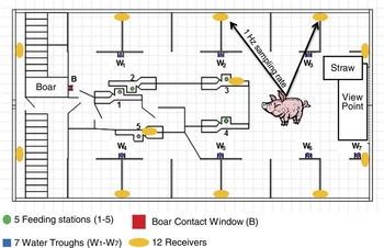
Data were acquired in the gestation sow unit of the Futterkamp research farm of the Chamber of Agriculture in Schleswig-Holstein, Germany, from April 2012 until May 2013. An overview of the gestation unit for 200 sows can be found in Figure 1. The general conditions of the barn are as follows: the central area for feeding and exercise has a slatted floor, whereas the 12 lying areas have a concrete floor. Feed is provided by five electronic feeding stations located in the central area. Depending on age and sows’ body condition, each sow has an individual feed demand. Daily feeding starts at 1900 h. Straw is provided in a rack in the running area. A boar pen is situated next to the running area. Sows are managed as a dynamic group meaning that new sows are integrated each week. For analysis purposes, data of 296 parities from 212 sows (84 sows with two parities) of gestation days 10 to 120 were used. Sow parities ranged between 2 and 5.
Overview of the gestation barn (floor area of 22×41 m), including the 12 receivers of the positioning system (mounted at about 2 m height). The gestation has 12 resting areas for 12 to 16 sows each. The five feeding stations are located in the central area.

Sensor system
In total, 212 cross-breed sows (Large White×Landrace) from two breeding organisations (A: 81 sows with 112 parities, B: 131 sows with 184 parities) were equipped with individual ear sensors, weighting <35 g and provided by MKW Electronics GmbH, Weibern, Austria. To sample the ear sensors’ position (x/y-coordinate) and acceleration (x, y, z-triples), 12 receivers were mounted at different positions in the gestation unit (Figure 1). The ear sensors actively sent a signal at a predefined sampling rate (e.g. every second, i.e. 1 Hz) to all receivers in range. The information of at least three receivers was necessary to calculate the position of the sow using the time of reception (difference between sending and receiving the signal).
The sampling rate of 1 Hz for the present data set resulted from limitations in battery life. Higher sampling rates (5 or 10 Hz) reduced battery life enormously; although lower sampling rates than 1 Hz reduced analysis accuracy (e.g. walked distance of animal). Further information on the sensor system can be found in Pichler et al. (Reference Pichler, Rudic, Breitenberger and Auer2014).
Lameness determination: treatments and scoring
To develop an automatic sow lameness detection system, two definitions of lame sows were used. First, during the observation period all treatments of lameness cases were documented by veterinarians and farm staff. All animals were checked once a day by farm staff and all lame animals were presented to a veterinarian. The day of diagnosis and detailed information on the severity was documented, for example front or hind leg, chronic or acute, if acute, for example, inflammation or abscess. Due to too few lameness treatments (38) in the statistical analysis, only the occurrence (yes/no) of a treatment could be considered.
Second, a lameness score was assigned once a week on the same day to all sows by two trained persons. The scoring system consisted of a three-point score from 0 to 2: 0 indicating sows with no obvious lameness; 1 describing sows with slight lameness; and 2 indicating sows with clearly visible lameness. In addition, the cause of lameness was to be documented using an adapted scoring system based on Main et al. (Reference Main, Clegg, Spatz and Green2000). The adapted scoring system included detailed information on claw length, claw wall ruptures and/or skin lesions above the claw. As only 46 sows received a score of 1 or 2 (122 scoring events), causes could not be considered in the statistical analysis.
Activity indices
Three activity indices were calculated per sow and day over the observation period. The indices ‘Path’ and ‘Square’ were derived from the positioning data. The index ‘acceleration’ was calculated using acceleration measurements.
Path length
Sampling the position of a sow that is not moving did not always produce the same x and y coordinates due to system precision. The coordinates scatter around the real value. Consequently, every nth signal the sows’ position was calculated using a moving average of the last m signals. Using this sequence of average positions, the daily path length walked by a sow was calculated as the Euclidean distance between two consecutive average positions. The total path length (S n,m ) was determined as the sum of all distances. The formula used to calculate the daily path length is given below (the variable ‘len’ stands for the number of positioning samples):
 $$\eqalign{ S_{{n,m}} {\equals}\mathop{\sum}\limits_{i\in\left\{ {2,2{\plus}n,2{\plus}2n,\,\ldots\,,\,len{\minus}m{\plus}1} \right\}} \cr{\sqrt {\left( {{1 \over m}\mathop \sum\limits_{j{\equals}i}^{m{\plus}i{\minus}1} x_{j} {\minus}{1 \over m}\mathop \sum\limits_{j{\equals}i{\minus}1}^{m{\plus}i{\minus}2} x_{j} } \right)^{2} \atop\cr{\plus}\left( {{1 \over m}\mathop \sum\limits_{j{\equals}i}^{m{\plus}i{\minus}1} y_{j} {\minus}{1 \over m}\mathop \sum\limits_{j{\equals}i{\minus}1}^{m{\plus}i{\minus}2} y_{j} } \right)^{2} } } $$
Positioning data of 1 day from six individually marked randomly chosen sows in May 2012 were used as calibration data set to parameterise n and m. The distance a sow walked was measured on video and compared with the calculated path length. Different values for m and n were tested (n varied from 5 to 400 with increments of 5, m from 50 to 400 with a step width of 1). In Supplementary Figure S1, for the six sows, all combinations of n and m with a match in path length measured using video recordings and calculated using positioning data are shown. Note that combinations of n and m outside the range shown did not lead to a match. For each sow multiple combinations of n and m lead to a match in path length, therefore the average values of n=40 and m=200 were chosen for further calculations.
The maximum number of 86 400 samplings/day (60 s×60 m×24 h×sampling rate of 1 Hz) was not achieved for all sows every day. Particularly, steel elements in the barn, such as pens separations, disturbed an optimal signal transfer. On average, 52 178 signals/day (SD=18 258.76) and a maximum number of 81 997 were reached. The data showed a linear relationship between the number of sampled positions per day and the distance walked (S n,m ). An example regression line is shown in Supplementary Figure S2a. To overcome a bias in the distance walked, data sets with <10 000 positions/sow and day were excluded and a sow-individual correction for the number of samples per day was carried out. A linear regression on the path length using historical data was performed for each sow and day. Samples from the last 15 days were used as historical data. The period 30 and 50 days was also tested but activity indices did not differ markedly (see example of a sow in Supplementary Figure S3). The average differences were diff30−15=0.0194 (SD=0.0170), diff50−30=0.0142 (SD=0.0128) and diff50−15=0.0283 (SD=0.0233). The shortest period of 15 days was chosen for the further calculations to minimise the need for data storage and calculation capacity. Using the regression coefficients, the corrected path length (S corr) was calculated (Supplementary Figure S2b – here for all sows and days together) and divided by the average corrected path length, the result being the activity index (Path) ranging around 1.
Using the regression coefficient from Supplementary Figure S2a and the average as shown in Supplementary Figure S2b, the resulting formula is
 $$\eqalign{ S_{{{\rm corr}}}\!= S_{{n,m}} {\minus}\left( {0.0108077{\times}{\rm number}\,{\rm of}\,{\rm samples}\,{\rm per}\,{\rm day}{\plus}93.2822} \right)\cr{\plus}583.9853 \cr \quad \qquad \qquad {\rm Path}\,{\equals}\,{{S_{{{\rm corr}}} } \over {583.9853} $$
The final activity index followed approximately a normal distribution and ranged around 1. The path lengths of 99 different sows on a total of 3783 days are plotted as examples in Supplementary Figures S2a and S2b. This normalisation procedure was executed for the path lengths of every individual sow. The regression lines as well as the mean path lengths of the different sows have a dynamic behaviour in time, so the model is time-invariant.
Squares
As a second activity index based on the positioning data, ‘Square’ describe the number of squares visited by a sow during a day. A lattice of 25×25 cm squares was laid on the area of the gestating unit. The square was determined for each x- and y-position. Again, a linear relationship between the number of squares visited and the number of positions per day was observed and a correction as well as normalisation was performed according to the path length.
Acceleration
The activity index acceleration was determined using the acceleration measurements. First, the variance of the acceleration measurements per sow and day was calculated. Similar to the path length and squares, the following steps were performed including a correction for the number of acceleration measurements per day and a normalisation using the sow-individual average of the last 15 days.
Statistical analysis
Due to the small number of 38 lameness treatments, statistical analysis was conducted in two steps. In the first step, activity indices were analysed using data from non-lame sows in a linear mixed model to determine influence factors. In a second step, differences were examined in the indices between non-lame and lame sows.
Non-lame sows
A linear mixed random regression model including an autocorrelation structure was used to analyse non-lame days of the sows (n=11 250). The model selection procedure was conducted following Kramer et al. (Reference Kramer, Stamer, Spilke, Thaller and Krieter2009). Information criteria were used for model selection, which is provided by default by the MIXED procedure (SAS Institute, 2014), to evaluate which fixed effects and twofold interactions should be included in the model. Model comparisons using the maximum likelihood principle were applied because information criteria based on the restricted maximum likelihood principle would not have been comparable as two models including different fixed effects were compared (Littell et al., Reference Littell, Milliken, Stroup, Wolfinger and Schabenberger2006). Akaike’s information criteria corrected (AICC, Hurvich and Tsai, Reference Hurvich and Tsai1989) and Bayesian information criteria (BIC, Schwarz, Reference Schwarz1978) were chosen as information criteria. These criteria take the number of estimated parameters into account and favour less complex model variants. The model with the smallest values for the AICC and BIC goodness-of-fit criteria was selected as the final model without considering the underlying significances of the effects.
In addition, a spatial (power) covariance structure (SP(POW)) for residuals was applied in the model. Repeated daily activity measurements within sow are assumed to contain interdependence and autocorrelated repeated measures (Littell et al., Reference Littell, Milliken, Stroup, Wolfinger and Schabenberger2006). Dependencies between residuals of repeated values can be modelled with covariance structures (Sawalha et al., Reference Sawalha, Keown, Kachman and van Vleck2005). For the SP(POW) structure, the correlations decline as a function of time and this type can handle unequally spaced data. The better the random regression model fits the data, the lower the correlation between residuals is expected to be. Hence, the model with the best fit was compared with the same model excluding the SP(POW) error covariance structure to confirm the estimated correlations between the residuals and thus verify the necessity of the error covariance structure.
The final model was the same for all three activity indices. As the gestating sows were managed as a dynamic group, test day was included as a fixed effect. Furthermore, the two breeding organisations (A and B) and the parity of the sows in classes (2nd, 3rd and 4th+5th parity) improved the model composition. The gestation day (days 10 to 120) was included as a linear covariate. The sow nested within breed was included as a random effect. Least square (LS) means were tested for significant differences using a t test with a Bonferroni correction to adjust for multiple comparisons. Residuals were inspected visually for normality and variance homogeneity.
Comparison of non-lame and lame days of the lame sows
Lameness treatments
During the whole observation period, 38 treatments were carried out because of lameness. These treatments were reduced to 19 different lameness events as treatments on consecutive days were defined as one lameness event. A clear distinction between lame and non-lame days is necessary however to compare non-lame with lame sows. Therefore, the lameness period was defined to start 14 days before the first treatment of a lameness event (day −14 until day −1, before treatment on day 0). This included the assumption that a clearly visible lameness event does not evolve for longer than 14 days. Thus, a 14-day period of non-lame days was defined before the lameness period (day −28 until day −15).
Lameness scoring
To analyse the lameness score, only clearly visible lame sows (score 2) were distinguished from non-lame sows (score 0 or 1) to focus mainly on clearly visible lameness. In total, 91 scores of 2 were assigned. Summarising consecutive scores of 2 to an event resulted in 59 different events. Similar to the procedure previously described for lameness treatments, a scoring assignment of 2 was used as criteria to define lame and non-lame periods of 14-day length each.
For both lameness definitions, a linear mixed model was set up to compare non-lame and lame periods. Due to technical problems in signal transmission of the sensor system not all lame and non-lame days for all lameness events were available. For the treatment data set, the median length of the lame period was 12 and 11 days of the non-lame period. For the scoring data set, the median length of the lame period was 12 and 9 days of the non-lame period. To test the influence of these gaps in the time series on model results non-lame periods were simulated. For each sow, 14 days of all non-lame days were randomly chosen and ordered and considered as non-lame period. This was repeated 100 times. Results were not different from model results using the original data. Consequently, statistical analysis was conducted using the original lame and non-lame periods. The treatment data set comprised of 403 and the scoring data set of 1161 observations, respectively.
According to the model selection procedure for the activity indices previously described, testing day, breeding organisation (A and B) and parity class (2, 3 and 4+5) were included as fixed effects, and gestation day (days 10 to 120) was included as a linear covariate. In addition, the days of the non-lame/lame period (day −28 until day 0) were included as a fixed effect. Again, dependencies between residuals of repeated values were modelled with a spatial exponential (SP(POW)) error covariance structure. LS means were tested for significant differences using a t test with a Bonferroni correction to adjust for multiple comparisons. Residuals were inspected visually for normality and variance homogeneity.
Results
Non-lame sows
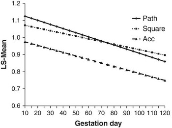
The effects test day and gestation day showed a significant influence on all activity indices (P<0.05). Parity class and breeding organisation were significant for Path and Acc. Sows of parities 4 and 5 walked less than sows of parity 2. Moreover, the acceleration was reduced with higher parity numbers. Sows of breeding organisation B had a shorter path length but higher acceleration than sows of breeding organisation A. LS means can be found in Table 1. Lower activity indices were observed for higher gestation days of a sow (Figure 2). Path decreased faster than the other indices. The index Acc was in general at a lower level than Path and Square.
Course of the activity indices: Path, Square and Acc depending on the linear covariate gestation day. n=11 250. Path=path length a sow walked during a day; Square=number of squares visited by a sow during a day in the barn; Acc=average acceleration at the sows’ ear; LS mean=least square mean.

Influence of the fixed effects parity class and breeding organisation on the activity indices Path, Square and Acc presented as least square (LS) means with standard errors

Path=path length a sow walked during a day; Square=number of squares visited by a sow during a day in the barn; Acc=average acceleration at the sows’ ear; n=number of animals.
a,bLS means with different superscripts differ significantly within activity index and effect: P<0.05.
Comparison of non-lame and lame days of the lame sows
Treatment
In the models comparing non-lame and lame periods of the sows, the gestation day influenced only the index Path significantly (P<0.05). Square and Acc were significantly influenced by the test day and the non-lame/lame period.
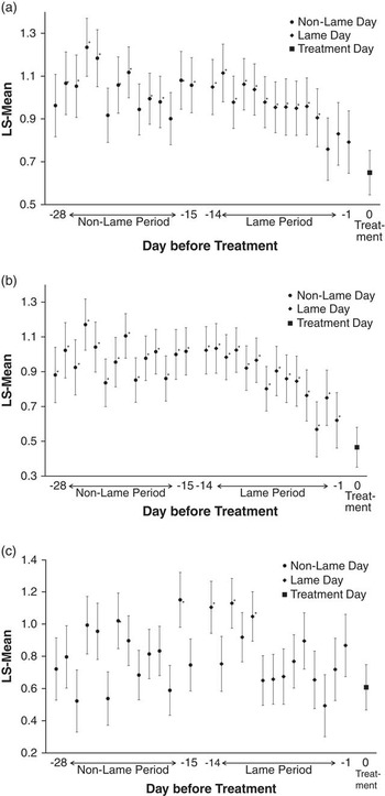
The influence of the non-lame/lame period on the activity indices is shown in Figure 3a and c. The indices Path and Square were lowest at the day of treatment. They decreased slightly in the days before treatment. Path did not differ significantly between the day of treatment and days −1 to −3, respectively. The majority of the other days in the lame period and the days in the non-lame period differed significantly (P<0.05) from the day of treatment. Within the non-lame period, the indices were at a higher level than the days before treatment, there was more variation between days, and no clear trend could be found. The activity index Acc showed different behaviour (Figure 3c). The non-lame period could not be distinguished from the lame period. Within both periods, the index varied from day to day and no trend could be found. Even at the day of treatment, the index was at a low but comparable level to the other days. Significant differences (P<0.05) from the day of treatment were found for days −22 and −16 of the non-lame period and days −14, −12 and −10 of the lame period.
Least square (LS) means and standard errors of the days of the non-lame and lame periods for the three activity indices: Path (a), Square (b) and Acc (c) when treatment was used to define lameness. Note that treatment was at day 0, lame period day −1 until day −14 and non-lame period day −15 until day −28. n=403. *Significant difference (P<0.05) to the day of treatment. Path=path length a sow walked during a day; Square=number of squares visited by a sow during a day in the barn; Acc=average acceleration at the sows’ ear.

Scoring
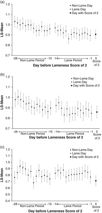
In the models analysing the lameness score, all indices were significantly influenced by the gestation day and the indices Square and Acc were also influenced by the test day. All other effects were not significant. Results of the non-lame/lame period are shown in Figure 4a and c. No clear trend or significant difference could be seen for the lame period or the days before a score of 2 was assigned. At the scoring date, the index was almost at the same level as during the whole lame period. Even compared with the non-lame period, it was mostly not significantly different. Most day-to-day variation could again be found for the index Acc. Compared with the Acc, the other indices were at a slightly but not significantly higher level during the non-lame period than in the lame period.
Least square (LS) means and standard errors of the days of the non-lame and lame periods for the three activity indices: Path (a), Square (b) and Acc (c) when a lameness score of 2 was used to define lameness. Note that treatment was at day 0, lame period day −1 until day −14 and non-lame period day −15 until day −28. n=1161. *Significant difference (P<0.05) to the day with score of 2. Path=path length a sow walked during a day; Square=number of squares visited by a sow during a day in the barn; Acc=average acceleration at the sows’ ear.

Discussion
Lameness evaluation
To evaluate an automatic lameness detection system, a reference is needed, which ideally represents the real situation or what is to be detected (Law, Reference Law2007). In the present study, two references were used, namely lameness treatment information and a lameness scoring system. All severely lame sows were presented to a veterinarian and treatments were recorded. Unfortunately, for the purposes of our study, only a few lame sows were observed. In the present study, for all lameness events, the 14-day period before the treatment was analysed. As the results show, a reduction in activity occurred mainly 3 or 4 days before the treatment. The period of 14 days was long enough to have a clear distinction between lame and non-lame days. The early detection of lameness was also expected to be possible with the scoring system. However, the weekly frequency of scoring was not sufficient. For future studies, a closer scoring scheme of every 2nd or 3rd day should be implemented.
Activity indices
The three activity indices were based on two different measuring systems. Path and Square, both based on positioning data, showed a decreasing trend during the 14-day period before treatment. Lame and non-lame periods could be distinguished. Before a score of 2, the decreasing trend was not as clear. Lame sows with a reduced activity could be identified using positioning data while acceleration measurements were not useful. Several studies stated that lame sows were affected in their feeding and drinking as well as social behaviour compared with non-lame sows. Sitting and lying could be observed more frequently, sows were less active (Díaz and Boyle, Reference Díaz and Boyle2014). Even studies on dairy cows have shown that lame cows in freestalls and at pasture have longer lying times than non-lame cows (e.g. Blackie et al., Reference Blackie, Bleach, Amory and Scaife2011). The causes were probably that pain affects the lying mechanism of the cow (Juarez et al., Reference Juarez, Robinson, DePeters and Price2003).
The acceleration index represented the variance in the acceleration measured at the ear of the sow. Studies with horses have shown that asymmetric head movements have a major role in lameness compensation (Vorstenbosch et al., Reference von Wachenfelt, Nilsson and Pinzke1997). Buchner et al. (Reference Buchner, Savelberg, Schamhardt and Barneveld1996) found a sinusoidal pattern in vertical displacement, velocity and acceleration for head, withers and tuber sacrale for non-lame horses, whereas lame horses with lameness at the forelimb expressed movement change much more at the head than at the withers. The reverse was true with hind limb lameness. Pluym et al. (Reference Pluym, Maes, Vangeyte, Mertens, Baert, van Weyenberg, Millet and van Nuffel2013b) described sows with a lameness in their hind leg showing more but shorter kicks when lifting the lame leg off the ground compared with non-lame sows. Lame animals will be less willing to exert force on the affected leg (Keegan et al., Reference Keegan, Wilson, Wilson, Smith, Gaughan, Pleasant, Lillich and Kramer1998; Corr et al., Reference Corr, McCorquodale, McGovern, Gentle and Bennett2003) and the weight is unevenly distributed (Wachenfelt et al., Reference Vorstenbosch, Buchner, Savelberg, Schamhardt and Barneveld2010; Sun et al., Reference Sun, Fitzgerald, Stalder, Karriker, Johnson and Hoff2011; Pluym et al., Reference Pluym, van Nuffel and Maes2013a). Assuming similar behaviour in lame sows, acceleration sensors in the ear might be able to measure differences in movements of lame and non-lame sows.
Linear models, as used in the present study, estimate average values for the lame and non-lame days of the sows. However, repeatabilities around 45% indicated that sows have individual activity patterns. Subsequent studies should take these sow’s individual activity patterns into account. Further improvement in the results would be expected using a sampling rate >1 Hz or by changing the time period. All three activity indices were calculated on a daily basis. As pigs have a circadian pattern in activity (McGlone and Newby, Reference McGlone and Newby1994), indices for shorter time intervals than a day should be evaluated. Changes in activity patterns during the day are possible. Lame animals might change their water and feed intake behaviour, for example time point or meal size. Time points and duration spend in other activities such as social interactions or interacting with enrichment material might also be different. Moreover, these changes are presumably accompanied by variations in visited areas in the barn. Shorter time intervals are expected to reflect these behavioural changes better than average daily values.
In conclusion, the use of ear sensors is an objective and easy-to-use method to detect changes in the activity pattern. Its utilisation is not limited to experimental farms. After installing the receiver system, it can be easily used in commercial farms too. Changes in the movement behaviour of lame sows are visible using differences between the activity indices based on positioning data. The acceleration seems to be less usable to detect lameness for time periods of a whole day. Furthermore, the indices should be validated using a data set with more lame sows.
Acknowledgements
This work has been financially supported by the Federal Office for Agriculture and Food (FKZ 2813700810). Grateful support was also provided by the Linz Center of Mechatronics in the framework of the Austrian COMET-K2 programme.
Supplementary material
For supplementary material/s referred to in this article, please visit http://dx.doi.org/doi:10.1017/S175173111500302X