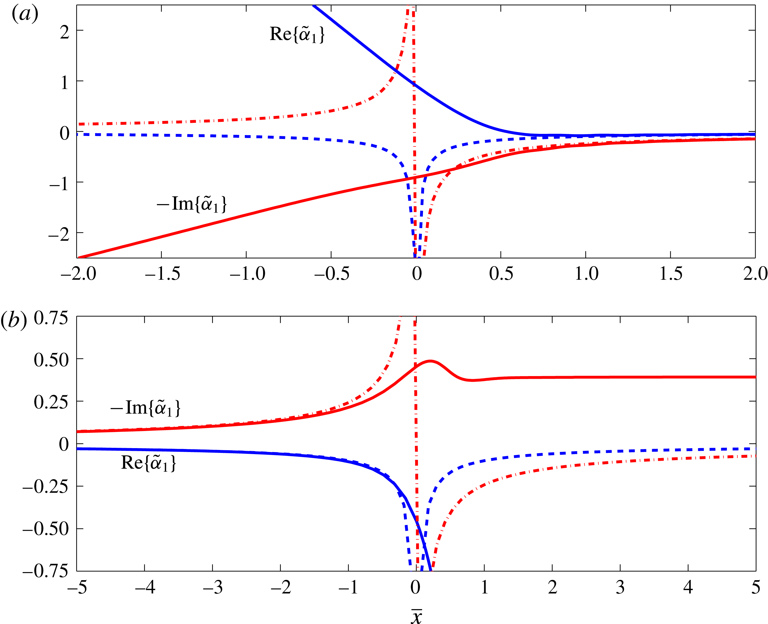
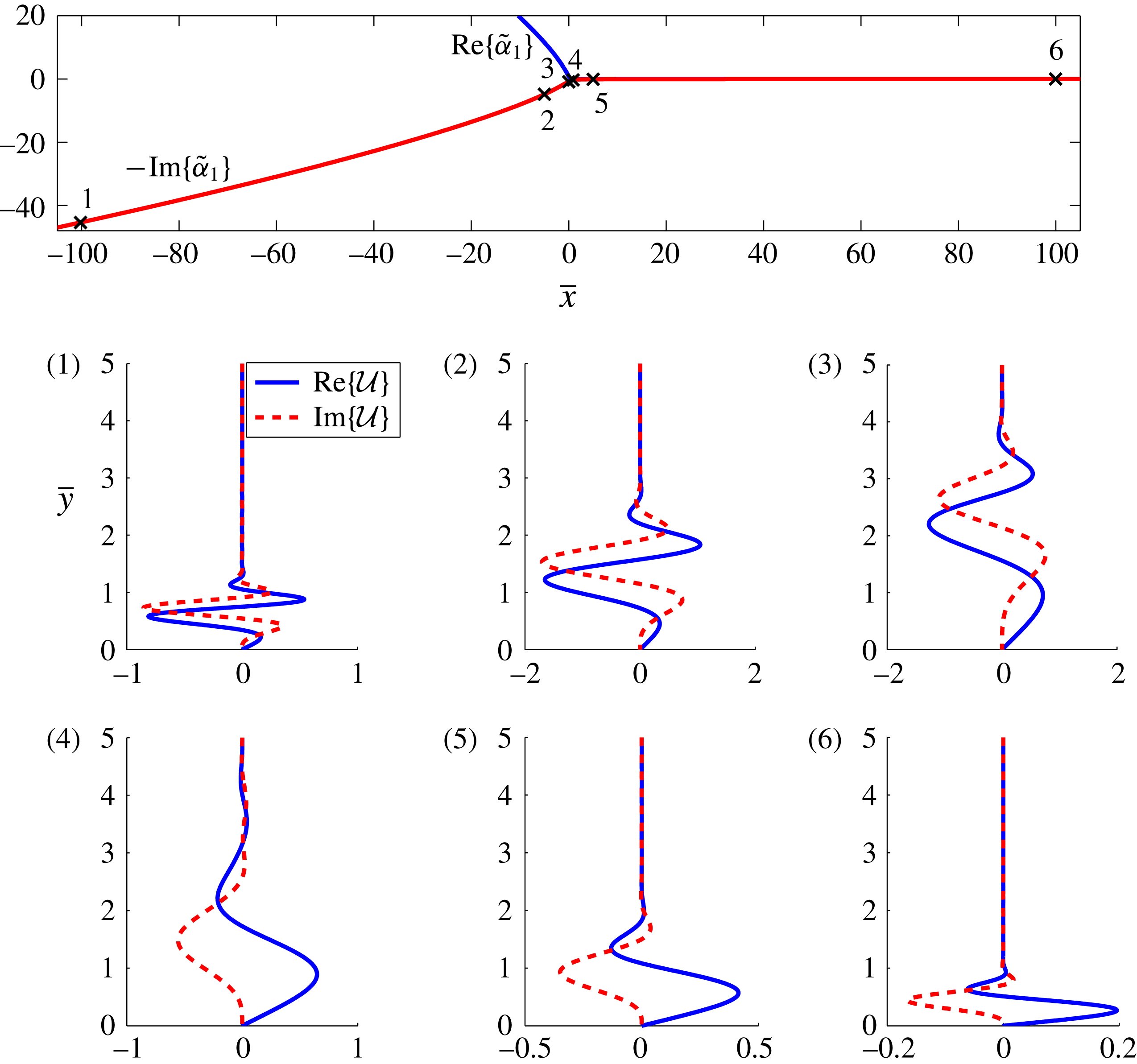
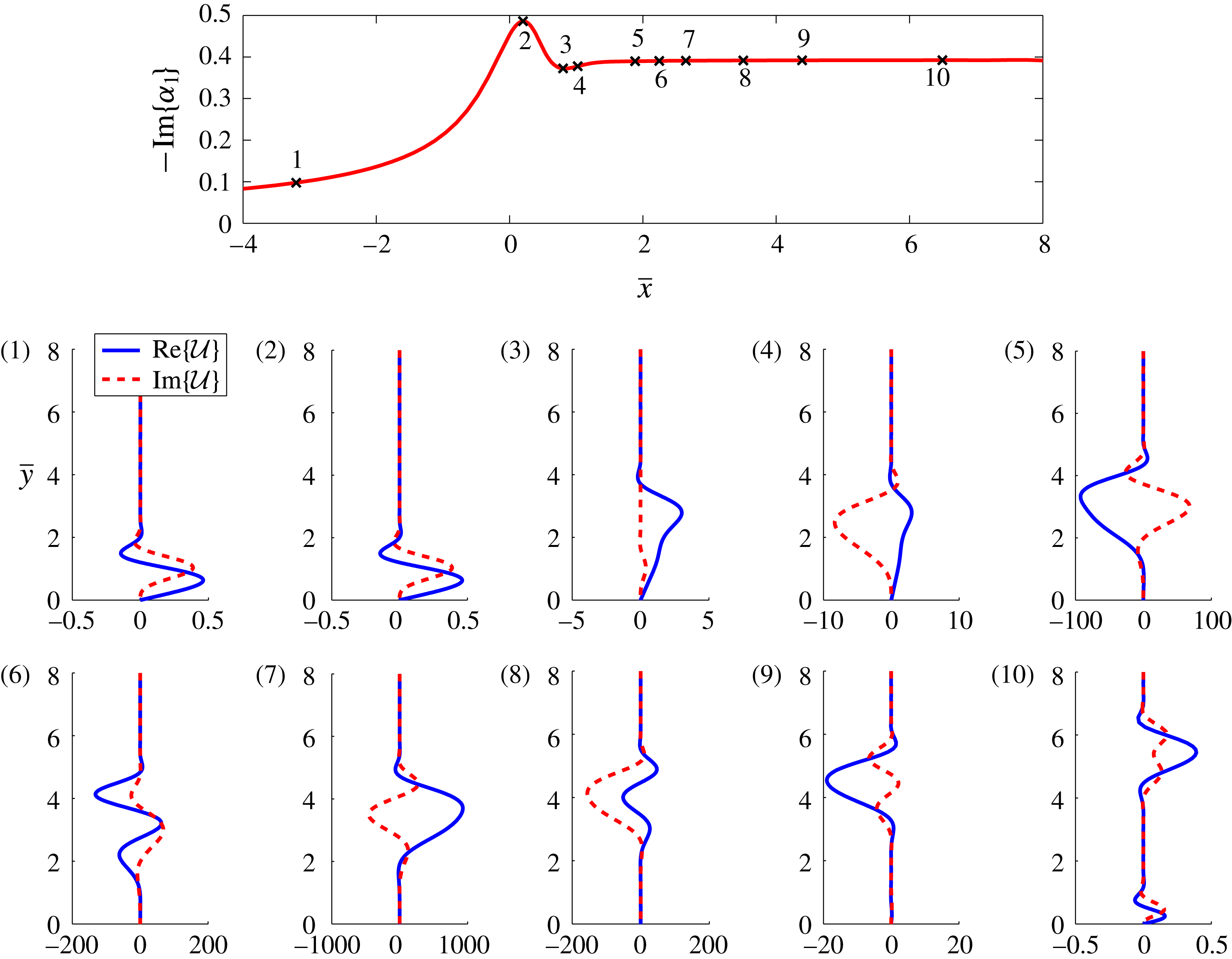
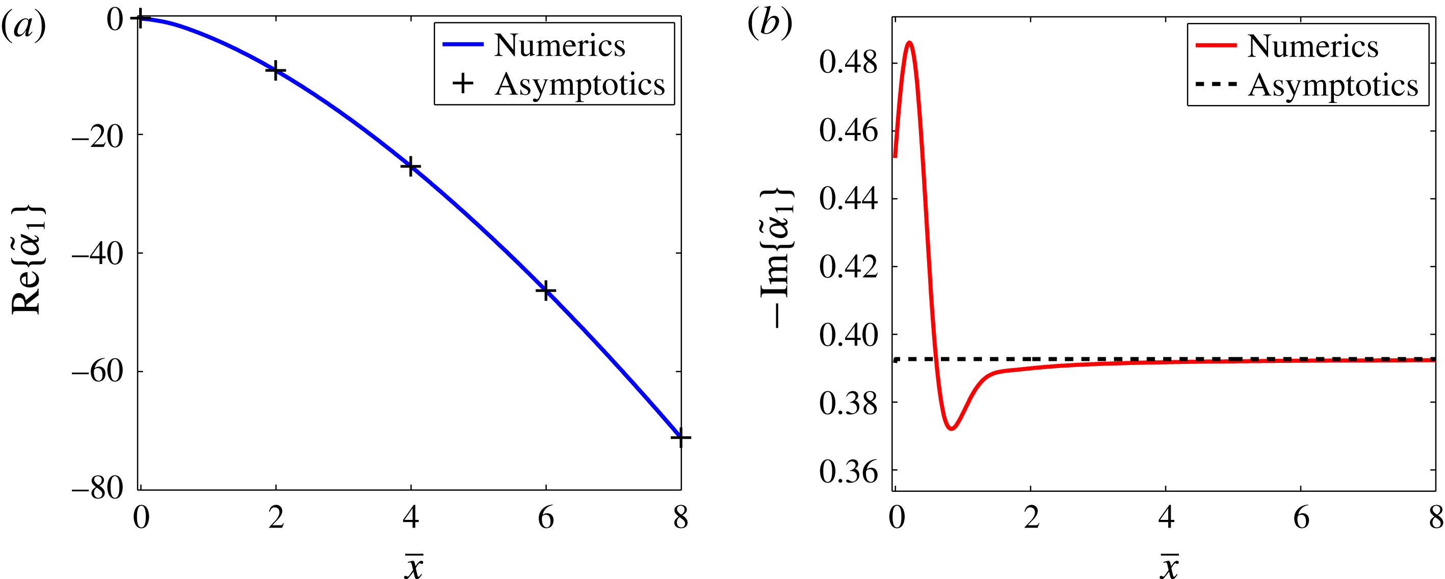
1 Introduction
Transition of high-Reynolds-number flows from a laminar state to turbulence involves a sequence of complex processes that are still not well understood. Transition to turbulence can substantially alter key flow quantities such as the volumetric flow rate, the total drag exerted on the boundaries, the heat conduction of the flow and, at high speed, aerodynamic heating. For flight, the turbulent boundary layer across the latter sections of the wing can produce as much as 10 times the drag of the corresponding laminar flow (Joslin Reference Joslin1998). It is thus desirable to design the wing such that the laminar portion of the boundary layer is maintained for as long as possible, in order to improve the fuel efficiency of the aircraft. This requires accurate transition-prediction methods, which in turn depend upon a detailed understanding of the physical processes involved.
When the external disturbance levels are low, transition of boundary layers typically starts with amplification of small disturbances owing to inherent instabilities. The subsequent development of the perturbed flow, aptly described by Morkovin, Reshotko & Herbert (Reference Morkovin, Reshotko and Herbert1994), involves nonlinear interaction and mean flow alteration, onset of rapidly growing secondary instabilities and final breakdown to a turbulent state. The characteristics of the transition process are thus highly dependent on the particular instabilities that have been excited. Of the four main linear instabilities that may occur in a swept-wing boundary layer – the attachment-line instability, the Tollmien–Schlichting (TS) instability, the Görtler instability and the crossflow instability – it is typically the last that plays the dominant role and is thus the main concern for modern wing designs (Bippes Reference Bippes1999; Saric, Reed & White Reference Saric, Reed and White2003). For studies of the instabilities that arise within the attachment-line region, and their connection to the crossflow instability, see Bertolotti (Reference Bertolotti2000a ) and Theofilis et al. (Reference Theofilis, Fedorov, Obrist and Dallmann2003).
The crossflow instability is a predominantly inviscid instability that operates in regions of favourable pressure gradient, and so is usually triggered close to the leading edge. The inviscid mechanism for the instability is set up by the pressure gradient and the three-dimensional nature due to the sweep of the wing. External to the boundary layer, the pressure gradient is balanced by the centrifugal force that arises as the fluid particles follow curved streamlines. Towards the wing surface, the streamwise velocity decreases to zero in order to satisfy the no-slip condition, but the pressure gradient remains constant at leading order. This imbalance generates a ‘crossflow’ velocity component, perpendicular to the local inviscid streamline. The velocity profile of this component is inflectional, and hence by Rayleigh’s inflection point theorem may admit an inviscid instability, as was first pointed out by Gregory, Stuart & Walker (Reference Gregory, Stuart and Walker1955) as part of their seminal study of the crossflow instability. Their work showed that the instability modes take two forms: travelling waves and stationary, co-rotating vortices.
The characteristics of both the travelling and stationary vortices have been determined numerically by solving the linearised stability equations for finite Reynolds numbers (Bippes, Müller & Wagner Reference Bippes, Müller and Wagner1991; Fischer & Dallmann Reference Fischer and Dallmann1991; Bippes Reference Bippes1999; Wassermann & Kloker Reference Wassermann and Kloker2003). Linear stability theory predicts larger growth rates for travelling vortices. However, stationary vortices tend to be dominant in the presence of low levels of free-stream disturbances, which are characteristic of the flight environment. This is due to the disparity in their amplitudes when they are first excited. Stationary vortices are most easily trigged by surface roughness, while travelling modes are excited by unsteady free-stream fluctuations, possibly through interactions with surface roughness. Since the free-stream disturbance levels in flight conditions are typically approximately
 $0.05\,\%$
of the free-stream velocity (Woodruff, Saric & Reed Reference Woodruff, Saric and Reed2011), the initial amplitudes of travelling waves are correspondingly much smaller than those of stationary vortices. Stationary vortices and the ensuing transition have thus received much more attention. However, wind tunnel experiments show that at elevated levels of free-stream turbulence, travelling vortices would prevail to cause transition (Müller Reference Müller1990; Dehyle & Bippes Reference Dehyle and Bippes1996). It is well recognised that external disturbances, such as surface roughness and free-stream turbulence, play a critical role in deciding transition paths and location. One of the mechanisms by which they influence transition is through exciting instability modes, i.e. the so-called receptivity, which is the very first stage of the transition route.
The primary focus of the present study will be on receptivity and linear instability near the leading edge of the wing. For completeness, we mention briefly works on, and our current understanding of, the subsequent stages. It has been observed that stationary vortices undergo prolonged nonlinear development, characterised by gradual saturation of their amplitude and emergence of complex spatial structures (Bippes et al.
Reference Bippes, Müller and Wagner1991; Reibert et al.
Reference Reibert, Saric, Carrillo and Chapman1996; Serpieri & Kotsonis Reference Serpieri and Kotsonis2016). These nonlinear behaviours have been captured by NPSE (nonlinear parabolised stability equations) calculations (Malik, Li & Chang Reference Malik, Li and Chang1994; Haynes & Reed Reference Haynes and Reed2000), nonlinear stability theory (Gajjar Reference Gajjar1996), and direct numerical simulation (DNS) (Wassermann & Kloker Reference Wassermann and Kloker2002; Duan, Choudhari & Li Reference Duan, Choudhari and Li2013). Due to their three-dimensional nature, crossflow vortices transfer low/high momentum away from/toward the surface of the wing, causing an
 $O(1)$
distortion to the background flow. The resulting velocity profile becomes inflectional in both the streamwise and spanwise directions, and as a result secondary instabilities occur, taking the flow to a turbulent state (Chernoray et al.
Reference Chernoray, Dovgal, Kozlov and Löfdahl2005; White & Saric Reference White and Saric2005; Serpieri & Kotsonis Reference Serpieri and Kotsonis2016). These have been confirmed by theoretical analysis (Högberg & Henningson Reference Högberg and Henningson1998; Malik et al.
Reference Malik, Li, Choudhari and Chang1999) and DNS (Bonfigli & Kloker Reference Bonfigli and Kloker2007; Duan et al.
Reference Duan, Choudhari and Li2013). Transition initiated by travelling vortices appears to follow a broadly similar route of nonlinear development and secondary instability (Wassermann & Kloker Reference Wassermann and Kloker2003; Li et al.
Reference Li, Choudhari, Duan and Chang2014). In order to delineate which modes cause transition and how the transition location depends quantitatively on surface roughness and free-stream disturbances, it is necessary to investigate receptivity to both.
Complementary to the finite-Reynolds-number numerical studies, large-Reynolds-number asymptotic analysis provides analytical insights into the essential mechanisms and salient features of the instability. The analysis of Choudhari (Reference Choudhari1994a
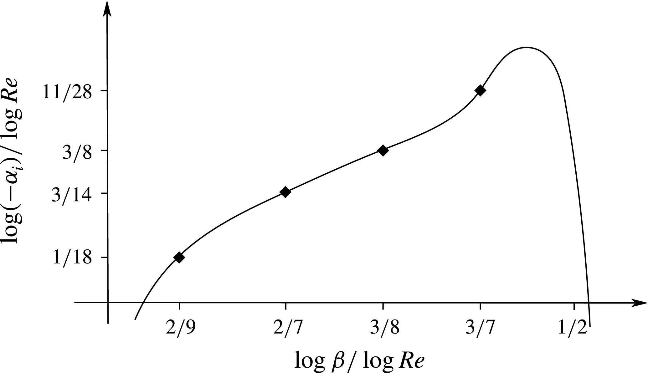
, Reference Choudhari1995) revealed that the linear amplification properties of stationary vortices fall into five distinct regimes. At a fixed streamwise location, these regimes are characterised by the spanwise wavenumber
 $\unicode[STIX]{x1D6FD}$
scaling as
 $$\begin{eqnarray}\displaystyle & \displaystyle \unicode[STIX]{x1D6FD}\sim Re^{\unicode[STIX]{x1D6FE}}, & \displaystyle\end{eqnarray}$$
where
 $\unicode[STIX]{x1D6FD}$
is non-dimensionalised by the chordwise distance
 $x^{\ast }$
from the leading edge, and
 $Re$
is the Reynolds number based on
 $x^{\ast }$
and the local streamwise slip velocity
 $Q_{s}^{\ast }$
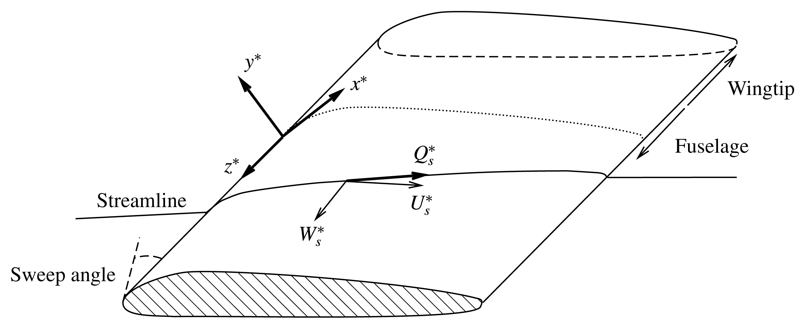
(see figure 2). The five regimes correspond to
 $\unicode[STIX]{x1D6FE}=1/2$
,
 $3/7$
,
 $3/8$
,
 $2/7$
and
 $2/9$
, and the respective growth rates scale as
 $-\unicode[STIX]{x1D6FC}_{i}\sim Re^{1/2}$
,
 $Re^{11/28}$
,
 $Re^{3/8}$
,
 $Re^{3/14}$
and
 $Re^{1/18}$
, as is shown in figure 1. An equivalent characterisation is that for a disturbance with a fixed physical spanwise wavelength, these regimes occur progressively closer to the leading edge of the wing – and so earlier on in the development of the vortices – as
 $\unicode[STIX]{x1D6FE}$
decreases.
Distinct linear instability regimes. The diagram is based on figure 6 from Choudhari (Reference Choudhari1995).

Swept-wing coordinate system.

The inviscid regime, first investigated by Gregory et al. (Reference Gregory, Stuart and Walker1955) in the context of rotating-disk boundary layers, corresponds to
 $\unicode[STIX]{x1D6FE}=1/2$
with the spanwise wavelength comparable to the local boundary-layer thickness, and so the instability is governed by Rayleigh’s equation. The axes of the resulting vortices make a finite angle with the local inviscid streamline. Importantly, the boundary-layer velocity projected in the direction of the wavenumber vector of the vortices plays the role of the effective base flow. Like the crossflow component, this has an inflection point and hence supports an inviscid instability. Viscous effects are present in a sublayer near the surface of the wing in order to satisfy the no-slip condition, but only provide an
 $O(Re^{-1/6})$
correction to the growth rate (Hall Reference Hall1986).
As
 $\unicode[STIX]{x1D6FE}$
decreases, the effects of viscosity become more important. The viscous-modified regime occurs at
 $\unicode[STIX]{x1D6FE}=3/7$
when the viscous sublayer produces a leading-order effect on the growth rate of the vortices while the wavelength remains unaltered at leading order (Choudhari Reference Choudhari1994a
, Reference Choudhari1995). At
 $\unicode[STIX]{x1D6FE}=3/8$
, this viscous contribution becomes as dominant as the inviscid, influencing both the growth rate and wavelength, and the eigenmode takes on the standard triple-deck structure. As
 $\unicode[STIX]{x1D6FE}$
is decreased further, or equivalently as we move closer to the leading edge and hence earlier in the development of the vortices with a fixed a spanwise wavelength, the vortices align themselves at leading order with the local wall shear at
 $\unicode[STIX]{x1D6FE}=2/7$
. The eigenmode now acquires a steady version of the marginally separated triple-deck structure (Goldstein, Leib & Cowley Reference Goldstein, Leib and Cowley1987).
In these four previously investigated regimes, which were inter-connected by Choudhari (Reference Choudhari1994a
, Reference Choudhari1995), non-parallel-flow effects merely provide higher-order corrections. Choudhari (Reference Choudhari1994a
) also investigated the
 $\unicode[STIX]{x1D6FE}=2/9$
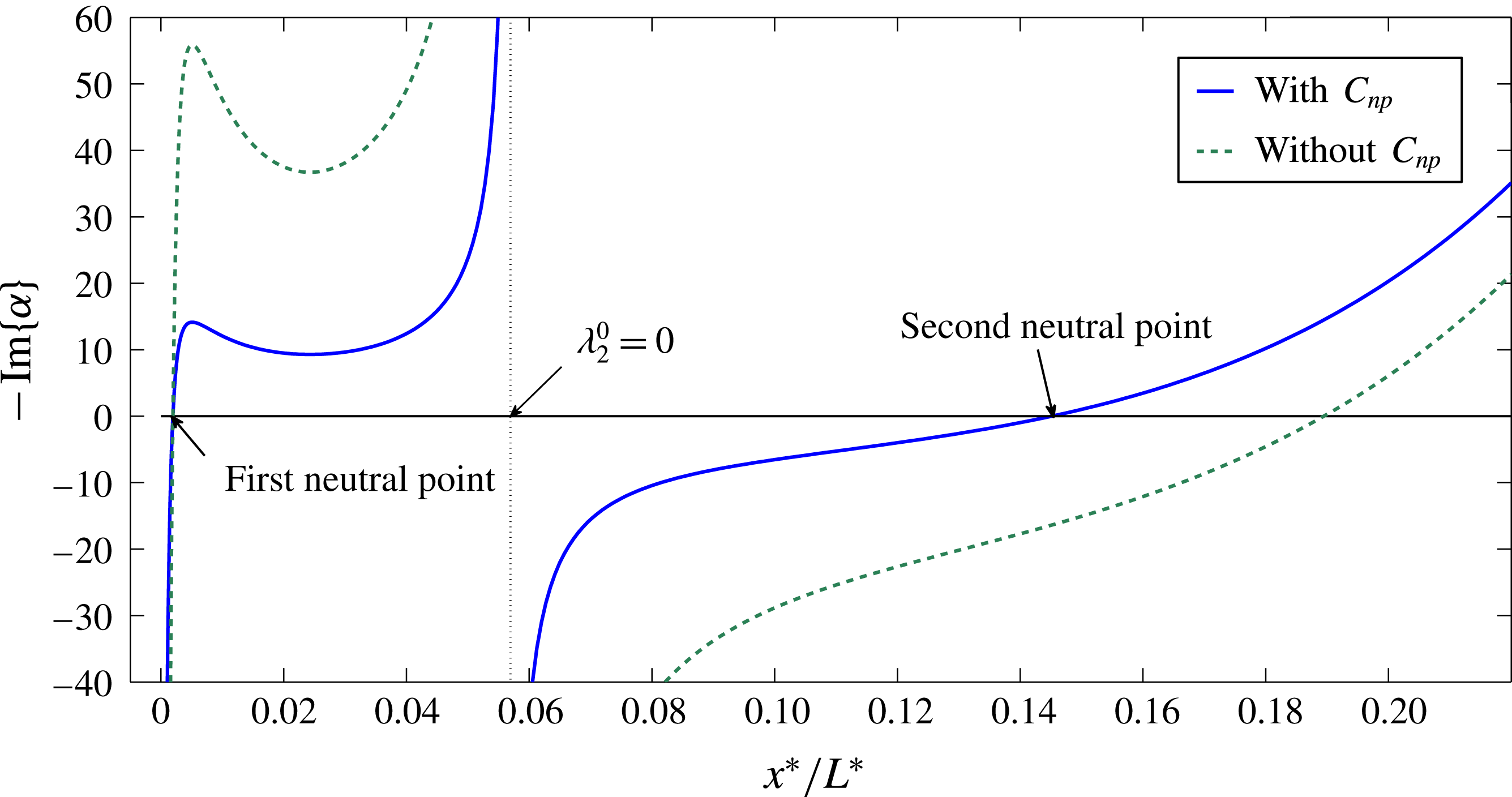
regime and described its asymptotic structure. However, his analysis started from the Orr–Sommerfeld (O–S) equation, which excluded non-parallelism at the outset. We will start with the linearised Navier–Stokes (N–S) equations, and show that non-parallelism in fact has a leading-order effect on the growth rate. This regime occurs closest to the leading edge since, as we will show later, it contains a neutral point, upstream of which the flow is stable. This regime therefore represents the genesis of the stationary crossflow instability, and the neutral modes constitute the lower branch of the neutral curve.
The generation of crossflow modes is thus expected to be most efficient here, in the region where they first become unstable: a mode generated upstream of this location will suffer from an initial region of decay, while one generated downstream of the neutral point will have a reduced region of growth within which to develop. The receptivity to external disturbances within this region is likely to determine which instability modes would dominate downstream. The most crucial issue of receptivity is to identify the so-called ‘scale tuning’ and/or ‘resonance condition’ mechanisms by which either the response adjusts its length scale, thereby evolving into an eigenmode, or external disturbances produce a forcing whose time and length scales match with those of the inherent instability. The seminal work of Goldstein (Reference Goldstein1983, Reference Goldstein1985) and Ruban (Reference Ruban1984), which was based on a high-Reynolds-number asymptotic framework and pertained to receptivity of a two-dimensional boundary layer to free-stream acoustic waves, showed that the required mechanisms can be provided by interactions of the acoustic wave with the rapidly varying base flow close to the leading edge, or with the local mean flow distortion caused by isolated surface roughness or curvature change. Since then, further receptivity mechanisms have been identified and described, including free-stream vortical disturbances interacting with isolated or distributed roughness (Duck, Ruban & Zhikharev Reference Duck, Ruban and Zhikharev1996; Wu Reference Wu2001a ,Reference Wu b ) and the direct interaction between acoustic and vortical fluctuations (Wu Reference Wu1999).
The experiments of Müller & Bippes (Reference Müller and Bippes1988) established the importance of surface roughness in the transition of three-dimensional (3-D) boundary layers. They found that the transition front for a stationary-vortex-dominated flow was fixed relative to their test model, and so a result of surface imperfections. Radeztsky, Reibert & Saric (Reference Radeztsky, Reibert and Saric1999) demonstrated that stationary vortices are remarkably sensitive to surface roughness, with micron-sized roughness, only a few per cent of the boundary-layer thickness in height, altering the transition location by as much as
 $20\,\%$
of the chord length. They also found that stationary crossflow vortices are most sensitive to roughness located near the leading edge (approximately
 $2\,\%$
of the chord length), with a weaker impact on the flow resulting from roughness placed further downstream. More recent experimental studies were carried out for a swept wing by Hunt & Saric (Reference Hunt and Saric2011) in wind tunnels and by Woodruff et al. (Reference Woodruff, Saric and Reed2011) in flight tests; see also Saric et al. (Reference Saric, West, Tufts and Reed2015). These measurements indicated a linear relation between the initial amplitude of vortices and the height of the micron-sized roughness arrays. Surprisingly, the receptivity appears to be affected by very moderate levels (approximately
 $0.02\,\%$
) of free-stream turbulence. Gaponenko et al. (Reference Gaponenko, Ivanov, Kachanov and Crouch2002) investigated generation by a local surface vibration in a boundary layer over a swept flat plate with the pressure gradient (required for the crossflow instability) being created by a contoured ceiling. They succeeded in obtaining comprehensive data on the coupling coefficient for a range of vibration frequencies and magnitudes. The results for surface roughness were extracted by extrapolating those for non-zero frequencies to the zero-frequency limit. It should be noted that this set-up probably does not capture the sensitivity to the roughness location exhibited by a swept wing because of the absence of an attachment line and the fact that the vibration is imposed fairly far downstream.
The mechanism for the generation of stationary vortices by surface roughness is, in comparison with the excitation of unsteady TS waves, somewhat simpler: 3-D roughness elements alone can trigger stationary modes, provided that their chordwise and spanwise length scales are comparable with those of the latter. Along this line, Choudhari & Streett (Reference Choudhari and Streett1990) and Choudhari (Reference Choudhari1994b ), among others, formulated a receptivity theory in terms of the O–S equation with an inhomogeneous boundary condition representing the forcing of small-amplitude surface roughness arrays, which were taken to be spanwise sinusoidal and chordwise localised. Implementing this approach, Ng & Crouch (Reference Ng and Crouch1999) calculated the amplitude of the vortices excited, which scales linearly with the roughness height as expected. Instead of this finite-Reynolds-number framework, Choudhari & Duck (Reference Choudhari and Duck1996) adapted the high-Reynolds-number asymptotic approach and investigated the receptivity of stationary vortices (in the inviscid regime) to roughness with height large enough for nonlinearity to be important. All of these theoretical studies ignored non-parallelism, which is indeed negligible in the region sufficiently downstream, but not necessarily so when close to the leading edge, as the present study will indicate. Non-parallelism was taken into account in the work of Bertolotti (Reference Bertolotti2000b ) by expanding the base flow as a Taylor series and the perturbation in terms of the small parameter characterising the streamwise variation of the base flow. The solution for the perturbation is found by numerically solving its governing equations in spectral space, and the amplitude of the crossflow mode was then determined by extracting numerically the residuals of relevant complex functions of the wavenumber. In this procedure, which is quite complicated, non-parallelism only provides a higher-order correction.
Simulations of receptivity to roughness elements located near the leading edge were carried out by Collis & Lele (Reference Collis and Lele1999), Rizzetta et al. (Reference Rizzetta, Visbal, Reed and Saric2010) and Kurz & Kloker (Reference Kurz and Kloker2014) using the linearised and full N–S equations, respectively. The first study found strong effects of non-parallelism, especially near the first (lower-branch) neutral point, highlighting the inadequacy of the stability and receptivity theory based on the O–S equation. The latter two studies emphasised the fact that roughness arrays generate a discrete set of stationary modes consisting of the fundamental component and its spanwise harmonics (since the spanwise Fourier transform of the roughness element shape is composed of these components). Kurz & Kloker (Reference Kurz and Kloker2014) observed a so-called ‘super-linearity’ behaviour of the receptivity, namely, the ratio of the amplitude of the excited fundamental vortices to the fundamental Fourier component of the roughness profile is a linear function of the roughness height rather than a constant. Tempelmann et al. (Reference Tempelmann, Schrader, Hanifi, Brandt and Henningson2012) set up DNS specifically to reproduce the experiments of Reibert et al. (Reference Reibert, Saric, Carrillo and Chapman1996), and the amplitude predicted by the computation was found to be approximately
 $40\,\%$
of the measurement.
One promising technique for delaying transition on swept wings has been the application of micron-sized spanwise-periodic discrete roughness elements (DREs), first proposed by Saric et al. (Reference Saric, Carrillo and Reibert1998), and its role as part of a laminar flow control procedure is discussed by Saric & Reed (Reference Saric and Reed2003). This technique exploits the sensitivity of receptivity to roughness near the leading edge or the attachment line. Such DREs are deployed to excite a stationary crossflow mode with the spanwise wavelength of the arrays, as well as higher harmonics, but no modes with larger wavelength. The spacing of the roughness is chosen to be smaller than the wavelength of the naturally most amplified mode, the critical mode. The DRE-generated, less unstable, shorter-wavelength modes inhibit the growth of the critical mode through modal interactions, but they themselves decay. Using NPSE, Atkin, Sunderland & Mughal (Reference Atkin, Sunderland and Mughal2006) and Li et al. (Reference Li, Choudhari, Chang, Streett and Carpenter2009, Reference Li, Choudhari, Chang, Streett and Carpenter2011) investigated the modal interactions, and the results confirmed the stabilising effects of the control mode. The latter two papers also performed secondary instability analysis, showing that the secondary instability is delayed and weakened, and recently Li et al. (Reference Li, Choudhari, Carpenter, Malik, Chang and Streett2016) took calculations to higher Reynolds numbers. In the calculations mentioned above, only a pure control mode with just a single pair of streamwise and spanwise wavenumbers was included, whereas in reality, DRE generates a packet of modes consisting of harmonics as well as the fundamental component. Wassermann & Kloker (Reference Wassermann and Kloker2002) performed DNS for different spectral compositions of the control modes, introduced via wall suction, and found that the spectral content does influence the nonlinear development, secondary instability and final onset of turbulence. Recently, Hosseini et al. (Reference Hosseini, Tempelmann, Hanifi and Henningson2013) carried out DNS, which included the receptivity of the flow to the DRE configuration of Saric et al. (Reference Saric, Carrillo and Reibert1998), and the result suggests that DRE is capable of delaying transition significantly. Despite these overwhelming positive computational results, flight test experiments have not been able to establish DRE as a viable laminar flow control technique (Saric et al. Reference Saric, West, Tufts and Reed2015), and a possible reason for the disagreement is that free-stream turbulence, though rather weak in the flight environment, may play a role (Downs & White Reference Downs and White2013).
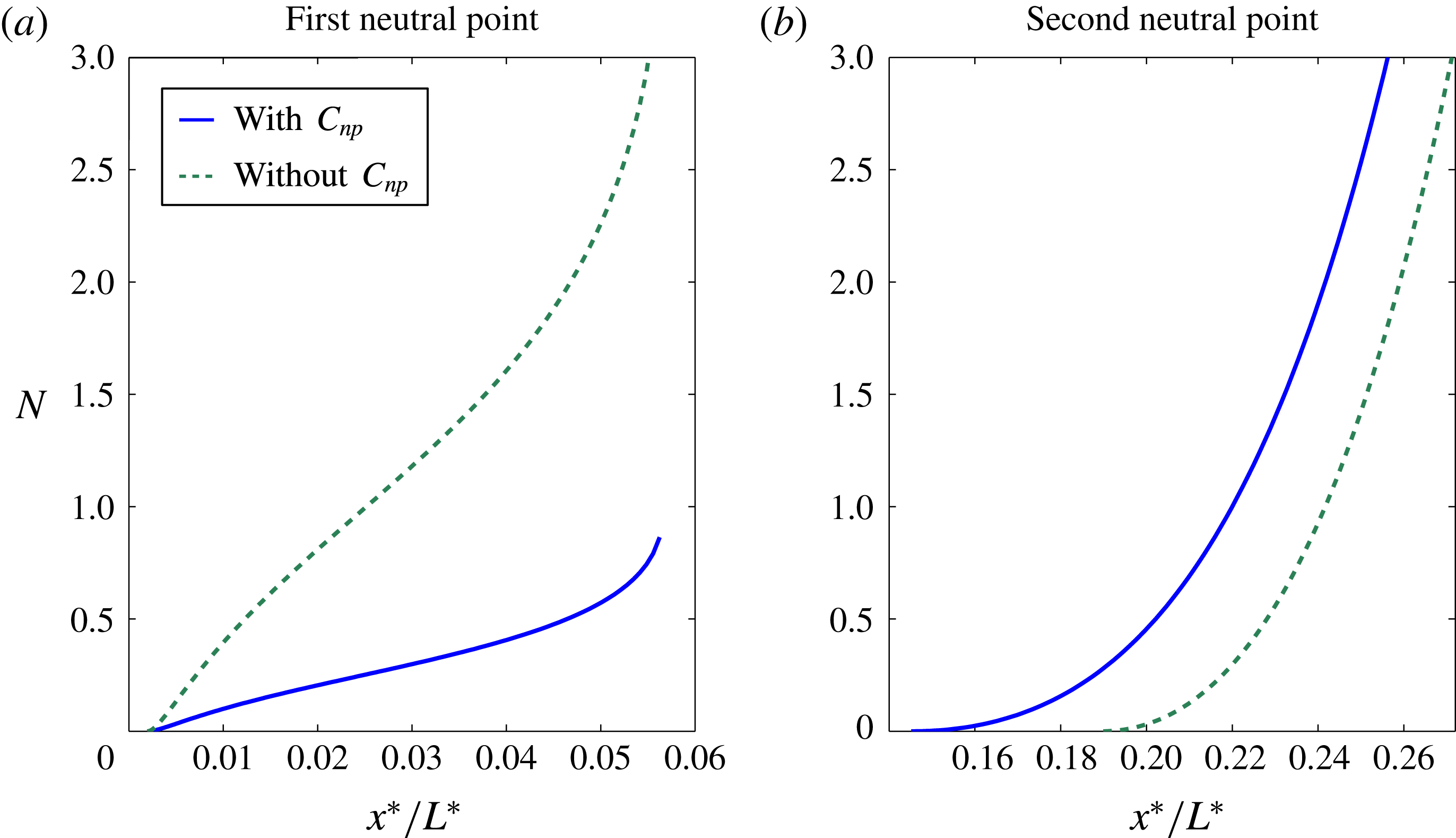
In summary, we may conclude that despite considerable work and progress on the instability and receptivity of swept-wing boundary layers, several issues remain to be addressed further, e.g. the super-linearity phenomenon and the substantial discrepancy between DNS and experiments. Much of the complication appears to be in the leading-edge region, and the non-parallel regime here is thus important. More specifically, the current most popular method for predicting the instability characteristics is by solving the O–S equation, in which non-parallelism is neglected, and the
 $N$
-factor measuring the accumulated amplification is found by integrating the growth rate from the neutral position. The accuracy of the growth rate and
 $N$
is thus dependent on non-parallel-flow effects being weak, and the neutral curve being determined precisely. When the more sophisticated method of parabolised stability equations (PSE) or NPSE is used, an initial condition has to be provided, usually by solving the O–S equation as well; the inaccuracy in the initial condition can affect the subsequent development. Furthermore, experiments have shown that lower-branch modes are extremely sensitive to surface roughness. If the instability is fundamentally changed by non-parallelism, then the receptivity theory must also be reformulated. It is thus prudent to investigate the effects of non-parallelism on instability and receptivity to surface roughness near the leading edge. Complementary to previous, mainly computational, efforts, we will take an analytical approach in order to shed light on possible intricacies that may arise. Our asymptotic approach is based on the large-Reynolds-number assumption and long-wavelength nature of the instability. To that end, we observe that in typical experiments, the chord length
 $L^{\ast }$
is usually approximately
 $2~\text{m}$
, and the Reynolds number based on
 $L^{\ast }$
is
 $2$
or
 $3$
million (while in flight it would be at least
 $10$
times as high). The roughness elements are typically located at
 $0.02L^{\ast }\approx 40~\text{mm}$
from the leading edge, where the boundary-layer thickness
 $\unicode[STIX]{x1D6FF}^{\ast }$
is a fraction of a millimetre. The spanwise spacing of the roughness elements is approximately
 $6$
–
 $12~\text{mm}$
, which is indeed much longer than
 $\unicode[STIX]{x1D6FF}^{\ast }$
.
We begin in § 3 with a large-Reynolds-number asymptotic analysis of the regime where non-parallelism has a leading-order effect on stationary vortices. This regime occurs close to the leading edge and contains a neutral point, and so represents the genesis of the instability. However, near the point where the pressure gradient is zero the analysis breaks down. We consider a localised region around this point in § 4, and identify a new instability as well as its connections to the instabilities upstream and downstream. In § 5, we return to the previous setting and consider the receptivity of the flow to surface roughness in the non-parallel regime. Finally, in § 6 we summarise our results, draw conclusions from them, and discuss potential avenues of research that follow on from the work presented here.
2 Problem formulation
In this paper we investigate stationary crossflow vortices, which arise due to the instability of the 3-D boundary layer over a swept wing. We use the body-fitted coordinate system depicted in figure 2;
 $x^{\ast }$
increases along the surface of the wing in the chordwise direction,
 $z^{\ast }$
in the spanwise direction and
 $y^{\ast }$
normal to the surface of the wing. Any curvature effects are to be neglected in order to focus on the effects of non-parallelism. As we are considering the local behaviour of the flow at some location a chordwise distance
 $x_{0}^{\ast }$
from the leading edge where the local streamwise slip velocity is
 $Q_{s,0}^{\ast }$
, we use these as our characteristic length and velocity, respectively. Along with the kinematic viscosity of the fluid
 $\unicode[STIX]{x1D708}^{\ast }$
, these characteristic scales give us the local Reynolds number
 $$\begin{eqnarray}\displaystyle & \displaystyle Re=Q_{s,0}^{\ast }x_{0}^{\ast }/\unicode[STIX]{x1D708}^{\ast }. & \displaystyle\end{eqnarray}$$
2.1 Base flow
We begin with our base flow
 $(\boldsymbol{U},P)=(U,Re^{-1/2}V,W,P)$
, which is a solution of the boundary-layer equations
 $$\begin{eqnarray}\displaystyle & \displaystyle UU_{x}+VU_{Y}+WU_{z}=-P_{x}+U_{YY}, & \displaystyle\end{eqnarray}$$
 $$\begin{eqnarray}\displaystyle & \displaystyle P_{Y}=0, & \displaystyle\end{eqnarray}$$
 $$\begin{eqnarray}\displaystyle & \displaystyle UW_{x}+VW_{Y}+WW_{z}=-P_{z}+W_{YY}, & \displaystyle\end{eqnarray}$$
 $$\begin{eqnarray}\displaystyle & \displaystyle U_{x}+V_{Y}+W_{z}=0, & \displaystyle\end{eqnarray}$$
subject to the boundary conditions
 $$\begin{eqnarray}\displaystyle & \displaystyle \boldsymbol{U}=\mathbf{0}\quad \text{at }Y=0,\quad (U,W)\rightarrow (U_{s},W_{s})\quad \text{as }Y\rightarrow \infty . & \displaystyle\end{eqnarray}$$
Here
 $Y=Re^{1/2}y$
is the
 $O(1)$
scaled vertical variable for the boundary layer, while
 $U_{s}$
and
 $W_{s}$
are the chordwise and spanwise slip velocities imposed by the inviscid flow external to the boundary layer. Since the pressure
 $P$
does not vary across the boundary layer, we can express it in terms of the slip velocities as
 $$\begin{eqnarray}\displaystyle & \displaystyle P_{x}=-U_{s}U_{s,x}-W_{s}U_{s,z},\quad P_{z}=-U_{s}W_{s,x}-W_{s}W_{s,z}. & \displaystyle\end{eqnarray}$$
Near the surface of the wing,
 $Y=0$
, each velocity component can be expressed as a Maclaurin series:
 $$\begin{eqnarray}\displaystyle & \displaystyle U\sim \mathop{\sum }_{n=1}^{\infty }\unicode[STIX]{x1D706}_{n}^{x}Y^{n},\quad V\sim \mathop{\sum }_{n=1}^{\infty }-\frac{1}{n+1}(\unicode[STIX]{x1D706}_{n,x}^{x}+\unicode[STIX]{x1D706}_{n,z}^{z})Y^{n+1},\quad W\sim \mathop{\sum }_{n=1}^{\infty }\unicode[STIX]{x1D706}_{n}^{z}Y^{n}, & \displaystyle\end{eqnarray}$$
where
 $\unicode[STIX]{x1D706}_{n}^{x}$
and
 $\unicode[STIX]{x1D706}_{n}^{z}$
are the Maclaurin coefficients for the series, given by
 $$\begin{eqnarray}\displaystyle \unicode[STIX]{x1D706}_{n}^{x}(x,z):=\left.\frac{1}{n!}\frac{\unicode[STIX]{x2202}^{n}U}{\unicode[STIX]{x2202}Y^{n}}\right|_{Y=0},\quad \unicode[STIX]{x1D706}_{n}^{z}(x,z):=\left.\frac{1}{n!}\frac{\unicode[STIX]{x2202}^{n}W}{\unicode[STIX]{x2202}Y^{n}}\right|_{Y=0}. & & \displaystyle\end{eqnarray}$$
Substituting (2.8) into (2.2) and (2.4) and collecting terms at each power of
 $Y$
gives the following relations:
 $$\begin{eqnarray}\displaystyle & \displaystyle 2\unicode[STIX]{x1D706}_{2}^{\phantom{x}}\hspace{0.0pt}^{\,{\displaystyle\mathop{x}\limits_{{\sim}}}}=-U_{s}\,{\displaystyle\mathop{ U}\limits_{{\sim}}}_{s,x}-W_{s}{\displaystyle\mathop{ U}\limits_{{\sim}}}_{s,z}, & \displaystyle\end{eqnarray}$$
 $$\begin{eqnarray}\displaystyle & \displaystyle 6\unicode[STIX]{x1D706}_{3}^{\phantom{x}}\hspace{0.0pt}^{\,{\displaystyle\mathop{x}\limits_{{\sim}}}}=0, & \displaystyle\end{eqnarray}$$
 $$\begin{eqnarray}\displaystyle & \displaystyle 24\unicode[STIX]{x1D706}_{4}^{\phantom{x}}\hspace{0.0pt}^{\,{\displaystyle\mathop{x}\limits_{{\sim}}}}=2\unicode[STIX]{x1D706}_{1}^{x}\unicode[STIX]{x1D706}_{1,x}^{\phantom{x}}\hspace{0.0pt}^{\,{\displaystyle\mathop{x}\limits_{{\sim}}}}+2\unicode[STIX]{x1D706}_{1}^{z}\unicode[STIX]{x1D706}_{1,z}^{\phantom{x}}\hspace{0.0pt}^{\,{\displaystyle\mathop{x}\limits_{{\sim}}}}-\unicode[STIX]{x1D706}_{1}^{\phantom{x}}\hspace{0.0pt}^{\,{\displaystyle\mathop{x}\limits_{{\sim}}}}(\unicode[STIX]{x1D706}_{1,x}^{x}+\unicode[STIX]{x1D706}_{1,z}^{z}). & \displaystyle\end{eqnarray}$$
In the ensuing analysis, there are often only minor differences between the corresponding chordwise and spanwise equations. We have thus introduced the simplifying notation
 ${\displaystyle\mathop{q}\limits_{{\sim}}}$
in (2.10)–(2.12), which we will make use of throughout this paper. In order to convert from the chordwise equation to its spanwise counterpart, one makes the substitutions
 $$\begin{eqnarray}\displaystyle \,{\displaystyle\mathop{x}\limits_{{\sim}}}\mapsto z,\quad \,{\displaystyle\mathop{U}\limits_{{\sim}}}\mapsto W,\quad \,{\displaystyle\mathop{u}\limits_{{\sim}}}\mapsto w. & & \displaystyle\end{eqnarray}$$
The right-hand side of (2.11) is zero because there is no imposed blowing or suction on the surface of the wing. The effects of blowing and suction on lower-branch modes have been considered in Choudhari (Reference Choudhari1994a ), where it was shown that even moderately weak suction could change the asymptotic scaling of the lower branch. Similarly, the non-parallel regime considered here is not present for the rotating-disk flow, due to the effects of the Coriolis force (Hall Reference Hall1986).
2.2 Instability modes
To the base flow
 $(\boldsymbol{U},P)$
, a perturbation
 $(\boldsymbol{u}^{\prime },p^{\prime })$
of size
 $\unicode[STIX]{x1D716}$
is introduced. Since we are considering the early development of the stationary crossflow instability, this perturbation is small, i.e.
 $\unicode[STIX]{x1D716}\ll 1$
. The perturbed flow can thus be expressed as
 $$\begin{eqnarray}\displaystyle & \displaystyle (\boldsymbol{u},p)=(\boldsymbol{U},P)+\unicode[STIX]{x1D716}(\boldsymbol{u}^{\prime }(x,Y,z),p^{\prime }(x,Y,z))+O(\unicode[STIX]{x1D716}^{2}). & \displaystyle\end{eqnarray}$$
The perturbation is governed by the linearised N–S equations,
 $$\begin{eqnarray}\displaystyle & \displaystyle (\boldsymbol{U}\boldsymbol{\cdot }\unicode[STIX]{x1D735})\boldsymbol{u}^{\prime }+(\boldsymbol{u}^{\prime }\boldsymbol{\cdot }\unicode[STIX]{x1D735})\boldsymbol{U}=-\unicode[STIX]{x1D735}p^{\prime }+Re^{-1}\unicode[STIX]{x1D6FB}^{2}\boldsymbol{u}^{\prime }, & \displaystyle\end{eqnarray}$$
 $$\begin{eqnarray}\displaystyle & \displaystyle \unicode[STIX]{x1D735}\boldsymbol{\cdot }\boldsymbol{u}^{\prime }=0, & \displaystyle\end{eqnarray}$$
subject to the no-slip and impermeability conditions,
 $$\begin{eqnarray}\displaystyle & \displaystyle \boldsymbol{u}^{\prime }=\mathbf{0}\quad \text{on }Y=0, & \displaystyle\end{eqnarray}$$
and the attenuation condition in the far field,
 $$\begin{eqnarray}\displaystyle & \displaystyle (\boldsymbol{u}^{\prime },p^{\prime })\rightarrow (\mathbf{0},0)\quad \text{as }Y\rightarrow \infty . & \displaystyle\end{eqnarray}$$
We seek solutions to this linear system in terms of its eigenmodes. Since the length scale over which the perturbation varies across the wing is much shorter than that for the base flow, the eigenmodes of the system take the WKB form
 $$\begin{eqnarray}\displaystyle & \displaystyle (\boldsymbol{u}^{\prime },p^{\prime })=(\tilde{\boldsymbol{u}},\tilde{p})(Y;x,z)\exp \left[\text{i}\left(\int _{0}^{x}\unicode[STIX]{x1D6FC}\,\text{d}\hat{x}+\unicode[STIX]{x1D6FD}z\right)\right]+\text{c.c.}, & \displaystyle\end{eqnarray}$$
where the chordwise and spanwise wavenumbers, denoted by
 $\unicode[STIX]{x1D6FC}$
and
 $\unicode[STIX]{x1D6FD}$
, are large. In the regimes of interest
 $$\begin{eqnarray}\displaystyle & \displaystyle \unicode[STIX]{x1D6FC},\unicode[STIX]{x1D6FD}\sim Re^{\unicode[STIX]{x1D6FE}}, & \displaystyle\end{eqnarray}$$
where
 $\unicode[STIX]{x1D6FE}$
is positive and takes different values depending on the regime considered. The value of
 $\unicode[STIX]{x1D6FE}$
is to be determined such that non-parallelism has a leading-order influence on the growth rate of the perturbation. Because the span of the wing is much larger than its chord length, the spanwise wavenumber
 $\unicode[STIX]{x1D6FD}=Re^{\unicode[STIX]{x1D6FE}}\unicode[STIX]{x1D6FD}_{0}$
is taken to be real and given, while the chordwise wavenumber
 $\unicode[STIX]{x1D6FC}$
is treated as a complex eigenvalue.
Hall (Reference Hall1986) showed for the rotating-disk flow that the wavefronts of lower-branch modes must be aligned with the local wall shear at leading order. By considering the limiting form of the dispersion relation for the triple-deck (
 $\unicode[STIX]{x1D6FE}=3/8$
) crossflow regime, Choudhari (Reference Choudhari1995) demonstrated that this also holds for swept-wing flows. The leading-order wavenumbers
 $Re^{\unicode[STIX]{x1D6FE}}\unicode[STIX]{x1D6FC}_{0}$
and
 $Re^{\unicode[STIX]{x1D6FE}}\unicode[STIX]{x1D6FD}_{0}$
are thus related through
 $$\begin{eqnarray}\displaystyle & \displaystyle \unicode[STIX]{x1D706}_{1}^{x}\unicode[STIX]{x1D6FC}_{0}+\unicode[STIX]{x1D706}_{1}^{z}\unicode[STIX]{x1D6FD}_{0}=0, & \displaystyle\end{eqnarray}$$
with
 $\unicode[STIX]{x1D706}_{1}^{x}$
and
 $\unicode[STIX]{x1D706}_{1}^{z}$
defined by (2.8). As a result of this, the rescaled leading-order chordwise wavenumber
 $\unicode[STIX]{x1D6FC}_{0}$
is real. In order to obtain the growth rate, it is necessary to take the analysis to a higher order and expand
 $\unicode[STIX]{x1D6FC}$
as
 $$\begin{eqnarray}\displaystyle & \displaystyle \unicode[STIX]{x1D6FC}=Re^{\unicode[STIX]{x1D6FE}}\unicode[STIX]{x1D6FC}_{0}+Re^{\unicode[STIX]{x1D6FE}_{np}}\unicode[STIX]{x1D6FC}_{1}+\cdots \,. & \displaystyle\end{eqnarray}$$
We thus wish to determine the correction
 $Re^{\unicode[STIX]{x1D6FE}_{np}}\unicode[STIX]{x1D6FC}_{1}$
to the chordwise wavenumber, which includes the leading-order contribution of non-parallelism to the growth rate.
The instability in this regime is, as expected, governed by the base-flow velocity projected in the direction of the leading-order wavenumber vector
 $(\unicode[STIX]{x1D6FC}_{0},\unicode[STIX]{x1D6FD}_{0})$
. This projection and its Maclaurin coefficients are defined as
 $$\begin{eqnarray}\displaystyle & \displaystyle U_{eff}:=U+\frac{\unicode[STIX]{x1D6FD}_{0}}{\unicode[STIX]{x1D6FC}_{0}}W, & \displaystyle\end{eqnarray}$$
 $$\begin{eqnarray}\displaystyle & \displaystyle \unicode[STIX]{x1D706}_{n}^{0}:=\unicode[STIX]{x1D706}_{n}^{x}+\frac{\unicode[STIX]{x1D6FD}_{0}}{\unicode[STIX]{x1D6FC}_{0}}\unicode[STIX]{x1D706}_{n}^{z}. & \displaystyle\end{eqnarray}$$
We can thus express the wall-shear alignment condition (2.21) as
 $$\begin{eqnarray}\displaystyle & \displaystyle \unicode[STIX]{x1D706}_{1}^{0}=0, & \displaystyle\end{eqnarray}$$
and (2.11), which holds in the absence of wall suction, as
 $\unicode[STIX]{x1D706}_{3}^{0}=0$
. Close to the surface of the wing, the effective base flow thus behaves as
 $$\begin{eqnarray}\displaystyle & \displaystyle U_{eff}\sim \unicode[STIX]{x1D706}_{2}^{0}Y^{2}+\unicode[STIX]{x1D706}_{4}^{0}Y^{4}+\cdots \quad \text{as }Y\rightarrow 0. & \displaystyle\end{eqnarray}$$
Since
 $\unicode[STIX]{x1D706}_{1}^{0}=0$
, the flow in the projected direction resembles a boundary-layer flow at the point of marginal separation (Goldstein et al.
Reference Goldstein, Leib and Cowley1987). This results in a marginally separated triple-deck structure for the perturbation: an ‘upper deck’ lies between the main boundary layer and the inviscid flow in order to account for the attenuation condition (2.18), while a thin, viscous ‘lower deck’ lies near the surface of the wing in order to satisfy the no-slip condition (2.17).
From (2.12) and (2.21), it follows that for any base flow with no imposed suction,
 $$\begin{eqnarray}\displaystyle & \displaystyle 12\unicode[STIX]{x1D706}_{4}^{0}=\unicode[STIX]{x1D706}_{1}^{x}\unicode[STIX]{x1D706}_{1,x}^{0}+\unicode[STIX]{x1D706}_{1}^{z}\unicode[STIX]{x1D706}_{1,z}^{0}, & \displaystyle\end{eqnarray}$$
where
 $$\begin{eqnarray}\displaystyle \unicode[STIX]{x1D706}_{n,{\displaystyle\mathop{x}\limits_{{\sim}}}}^{0}:=\unicode[STIX]{x1D706}_{n,{\displaystyle\mathop{x}\limits_{{\sim}}}}^{x}+\frac{\unicode[STIX]{x1D6FD}_{0}}{\unicode[STIX]{x1D6FC}_{0}}\unicode[STIX]{x1D706}_{n,{\displaystyle\mathop{x}\limits_{{\sim}}}}^{z}. & & \displaystyle\end{eqnarray}$$
2.3 Wavenumber scalings
We now present a scale analysis to fix
 $\unicode[STIX]{x1D6FE}$
and
 $\unicode[STIX]{x1D6FE}_{np}$
. Choudhari (Reference Choudhari1994a
) derived these by balancing the pressure gradient with the contribution to the inertia from the
 $O(Y^{4})$
term in
 $U_{eff}$
(see (2.26)). We will instead focus on the inclusion of non-parallelism in the governing equation for the perturbation.
As with the neighbouring instability regimes, a triple-deck structure arises (Choudhari Reference Choudhari1994a
). The lower-deck thickness is set by the balance of the inertial and viscous terms,
 $\unicode[STIX]{x1D6FC}U_{eff}u^{\prime }\sim u_{YY}^{\prime }$
. Since
 $\unicode[STIX]{x1D6FC}\sim Re^{\unicode[STIX]{x1D6FE}}$
,
 $U_{eff}\sim \unicode[STIX]{x1D706}_{2}^{0}Y^{2}$
by (2.26), and
 $u_{YY}^{\prime }\sim u^{\prime }\,Y^{-2}$
, it follows for
 $\unicode[STIX]{x1D706}_{2}^{0}=O(1)$
that
 $$\begin{eqnarray}\displaystyle & \displaystyle Y\sim Re^{-\unicode[STIX]{x1D6FE}/4}. & \displaystyle\end{eqnarray}$$
As the base-flow Maclaurin series proceeds in powers of
 $Y$
, we similarly expand
 $u^{\prime }$
as an asymptotic series in powers of
 $Re^{-\unicode[STIX]{x1D6FE}/4}$
, i.e.
 $u^{\prime }=\bar{u}_{0}+Re^{-\unicode[STIX]{x1D6FE}/4}\bar{u}_{1}+\cdots \,$
, etc.
Due to the interactive nature of the triple-deck structure, the behaviour of the perturbation is governed by the lower-deck equation for
 $v^{\prime }$
that contains the self-induced pressure perturbation
 $p^{\prime }$
. The scaling for the chordwise and spanwise wavenumbers is thus set by the requirement that in the lower deck the chordwise pressure gradient balances with the non-parallel variations of the flow,
 $\unicode[STIX]{x1D6FC}p^{\prime }\sim u^{\prime }U_{x}$
. Since
 $U_{x}\sim Y\sim Re^{-\unicode[STIX]{x1D6FE}/4}$
in the lower deck, we have
 $p^{\prime }\sim Re^{-5\unicode[STIX]{x1D6FE}/4}u^{\prime }$
. In triple-deck structures, the pressure perturbation does not vary across the lower or main deck at leading order. It must also be the same size as the vertical velocity perturbation in the main deck,
 $p^{\prime }\sim v^{\prime }$
, so that in the upper deck the pressure gradient can balance with both the vertical and horizontal momenta. Since the continuity equation (2.16) gives us that
 $v^{\prime }\sim yu_{x}^{\prime }$
, the pressure perturbation thus scales as
 $p^{\prime }\sim v^{\prime }\sim Re^{\unicode[STIX]{x1D6FE}-1/2}u^{\prime }$
in the main and lower decks. Equating these two pressure scalings, we find that
 $$\begin{eqnarray}\displaystyle & \displaystyle \unicode[STIX]{x1D6FE}={\displaystyle \frac{2}{9}}. & \displaystyle\end{eqnarray}$$
The scaling for the correction to the chordwise wavenumber is set by requiring that the corresponding inertial term also balances with the pressure term,
 $Re^{\unicode[STIX]{x1D6FE}_{np}}\unicode[STIX]{x1D6FC}_{1}\unicode[STIX]{x1D706}_{1}^{x}Yu^{\prime }\sim \unicode[STIX]{x1D6FC}p^{\prime }$
. Now, in the main deck we find that
 $v^{\prime }\propto U_{eff}$
at leading order. Because of the marginally separated nature of the effective base-flow profile, the matching condition from the main deck thus imposes that in the lower deck
 $v^{\prime }\sim Re^{\unicode[STIX]{x1D6FE}-1/2}Y^{2}u^{\prime }\sim Re^{(\unicode[STIX]{x1D6FE}-1)/2}u^{\prime }$
, which is
 $Re^{-\unicode[STIX]{x1D6FE}/4}$
smaller than the scaling suggested by the continuity equation. This means that
 $v^{\prime }$
does not appear at leading order in the lower-deck continuity equation, and so the inertial term above must involve the sub-leading-order term
 $\bar{u}_{1}$
in order to make a non-zero contribution to the combined momentum equation. The balance between inertia and non-parallelism thus becomes
 $Re^{\unicode[STIX]{x1D6FE}_{np}}\unicode[STIX]{x1D6FC}_{1}\unicode[STIX]{x1D706}_{1}^{x}Y(Re^{-\unicode[STIX]{x1D6FE}/4}\bar{u}_{1})\sim Re^{\unicode[STIX]{x1D6FE}}\unicode[STIX]{x1D6FC}_{0}p^{\prime }$
, and so
 $$\begin{eqnarray}\displaystyle & \displaystyle \unicode[STIX]{x1D6FE}_{np}={\displaystyle \frac{\unicode[STIX]{x1D6FE}}{4}}={\displaystyle \frac{1}{18}}. & \displaystyle\end{eqnarray}$$
For these scalings the inertial term
 $\unicode[STIX]{x1D6FC}\unicode[STIX]{x1D706}_{4}^{x}Y^{4}(Re^{-\unicode[STIX]{x1D6FE}/4}\bar{u}_{1})$
also balances with the pressure term, in agreement with Choudhari (Reference Choudhari1994a
). Our alternative arguments emphasise the importance of non-parallelism within this regime, some preliminary results about which were presented in Butler & Wu (Reference Butler and Wu2015).
3 Lower-branch regime: the role of non-parallelism
3.1 Main deck
We first consider the main deck, where
 $Y=O(1)$
. Without loss of generality, we can take
 $u^{\prime }$
and
 $w^{\prime }$
to be
 $O(1)$
quantities. Balancing the terms within the continuity equation, (2.16), tells us that
 $$\begin{eqnarray}\displaystyle & \displaystyle \text{i}Re^{2/9}(\unicode[STIX]{x1D6FC}_{0}+\cdots \,)u^{\prime }\sim Re^{1/2}v^{\prime }\sim \text{i}Re^{2/9}\unicode[STIX]{x1D6FD}_{0}w^{\prime }, & \displaystyle\end{eqnarray}$$
and so
 $$\begin{eqnarray}\displaystyle & \displaystyle v^{\prime }\sim Re^{-5/18}. & \displaystyle\end{eqnarray}$$
Thus the velocity and pressure of our eigenmode (2.19) are scaled as
 $$\begin{eqnarray}\displaystyle & \displaystyle (\tilde{\boldsymbol{u}},\tilde{p})=(\tilde{u} ,\unicode[STIX]{x1D700}^{5}\tilde{v},\tilde{w},\unicode[STIX]{x1D700}^{5}\tilde{p}), & \displaystyle\end{eqnarray}$$
where the small parameter
 $\unicode[STIX]{x1D700}$
is defined as
 $$\begin{eqnarray}\displaystyle & \displaystyle \unicode[STIX]{x1D700}:=Re^{-1/18}, & \displaystyle\end{eqnarray}$$
and we expand each of the flow components as asymptotic series:
 $(\tilde{\boldsymbol{u}},\tilde{p})=\sum _{j}\unicode[STIX]{x1D700}^{j}(\tilde{\boldsymbol{u}}_{j},\tilde{p})$
. We proceed by substituting this form of the perturbation into the linearised N–S equations (2.15)–(2.16) and boundary conditions (2.15)–(2.18), and solving the resulting equations at each order of
 $\unicode[STIX]{x1D700}$
.
At the orders that are relevant to our analysis, the
 ${\displaystyle\mathop{x}\limits_{{\sim}}}$
-momentum equation gives
 $$\begin{eqnarray}\displaystyle & \displaystyle 0=\text{i}\unicode[STIX]{x1D6FC}_{0}U_{eff}\,\tilde{{\displaystyle\mathop{u}\limits_{{\sim}}}}_{\,j}+\tilde{v}_{j}\,{\displaystyle\mathop{ U}\limits_{{\sim}}}_{Y}, & \displaystyle\end{eqnarray}$$
 $$\begin{eqnarray}\displaystyle & \displaystyle 0=\text{i}\unicode[STIX]{x1D6FC}_{0}U_{eff}\,\tilde{{\displaystyle\mathop{u}\limits_{{\sim}}}}_{3}+\text{i}\unicode[STIX]{x1D6FC}_{1}U\,\tilde{{\displaystyle\mathop{u}\limits_{{\sim}}}}_{0}+\tilde{v}_{3}\,{\displaystyle\mathop{ U}\limits_{{\sim}}}_{Y}, & \displaystyle\end{eqnarray}$$
where
 $j\in \{0,1,2\}$
. As usual, the
 $y$
-momentum equation reduces to
 $\tilde{p}_{k,Y}=0$
, and so the pressure perturbation is constant across the main deck, at the orders we are considering. Finally, the continuity equation (2.16) gives
 $$\begin{eqnarray}\displaystyle & \displaystyle 0=\text{i}\unicode[STIX]{x1D6FC}_{0}\tilde{u} _{j}+\tilde{v}_{j,Y}+\text{i}\unicode[STIX]{x1D6FD}_{0}\tilde{w}_{j}, & \displaystyle\end{eqnarray}$$
 $$\begin{eqnarray}\displaystyle & \displaystyle 0=\text{i}\unicode[STIX]{x1D6FC}_{0}\tilde{u} _{3}+\text{i}\unicode[STIX]{x1D6FC}_{1}\tilde{u} _{0}+\tilde{v}_{3,Y}+\text{i}\unicode[STIX]{x1D6FD}_{0}\tilde{w}_{3}. & \displaystyle\end{eqnarray}$$
We solve these at each order by using the continuity equation to combine the
 $x$
- and
 $z$
-momentum equations, leaving an equation for
 $\tilde{v}_{k}$
. We find that
 $$\begin{eqnarray}\displaystyle \tilde{{\displaystyle\mathop{u}\limits_{{\sim}}}}_{\,j}=A_{j}(x,z)\,{\displaystyle\mathop{ U}\limits_{{\sim}}}_{Y},\quad \tilde{v}_{j}=-\text{i}\unicode[STIX]{x1D6FC}_{0}A_{j}(x,z)U_{eff},\quad \tilde{p}_{j}=P_{j}(x,z), & & \displaystyle\end{eqnarray}$$
for
 $j=0,1,2$
, while
 $$\begin{eqnarray}\displaystyle \tilde{{\displaystyle\mathop{u}\limits_{{\sim}}}}_{3}=A_{3}(x,z)\,{\displaystyle\mathop{ U}\limits_{{\sim}}}_{Y},\quad \tilde{v}_{3}=-\text{i}\unicode[STIX]{x1D6FC}_{0}A_{3}(x,z)U_{eff}-\text{i}\unicode[STIX]{x1D6FC}_{1}A_{0}(x,z)U,\quad \tilde{p}_{3}=P_{3}(x,z), & & \displaystyle \nonumber\\ \displaystyle & & \displaystyle\end{eqnarray}$$
where the as-yet-unknown displacement functions
 $A_{k}(x,z)$
and pressure functions
 $P_{k}(x,z)$
will be related through the upper deck.
Non-parallelism appears in the main-deck solution at the next order in the expansions. However, we can show that
 $\tilde{v}_{4}\sim Y$
as
 $Y\rightarrow 0$
, and so the
 $O(\unicode[STIX]{x1D700}^{4})$
solution does not contribute to the matching conditions needed to determine the growth rate.
To facilitate matching, we note that these main-deck solutions have the following behaviours for small and large
 $Y$
. As
 $Y\rightarrow 0$
,
 $$\begin{eqnarray}\displaystyle & & \displaystyle \displaystyle \tilde{{\displaystyle\mathop{u}\limits_{{\sim}}}}\sim A_{0}(\unicode[STIX]{x1D706}_{1}^{\phantom{x}}\hspace{0.0pt}^{\,{\displaystyle\mathop{x}\limits_{{\sim}}}}+2\unicode[STIX]{x1D706}_{2}^{\phantom{x}}\hspace{0.0pt}^{\,{\displaystyle\mathop{x}\limits_{{\sim}}}}Y+\cdots \,)+\unicode[STIX]{x1D700}A_{1}(\unicode[STIX]{x1D706}_{1}^{\phantom{x}}\hspace{0.0pt}^{\,{\displaystyle\mathop{x}\limits_{{\sim}}}}+\cdots \,)+\unicode[STIX]{x1D700}^{2}A_{2}(\unicode[STIX]{x1D706}_{1}^{\phantom{x}}\hspace{0.0pt}^{\,{\displaystyle\mathop{x}\limits_{{\sim}}}}+\cdots \,)\nonumber\\ \displaystyle & & \displaystyle \quad +\,\unicode[STIX]{x1D700}^{3}A_{3}(\unicode[STIX]{x1D706}_{1}^{\phantom{x}}\hspace{0.0pt}^{\,{\displaystyle\mathop{x}\limits_{{\sim}}}}+\cdots \,)+\cdots \,,\end{eqnarray}$$
 $$\begin{eqnarray}\displaystyle & & \displaystyle \displaystyle \unicode[STIX]{x1D700}^{5}\tilde{v}\sim \unicode[STIX]{x1D700}^{5}(-\text{i}\unicode[STIX]{x1D6FC}_{0}A_{0}(\unicode[STIX]{x1D706}_{2}^{0}Y^{2}+\cdots \,))+\unicode[STIX]{x1D700}^{6}(-\text{i}\unicode[STIX]{x1D6FC}_{0}A_{1}(\unicode[STIX]{x1D706}_{2}^{0}Y^{2}+\cdots \,))+\unicode[STIX]{x1D700}^{7}(-\text{i}\unicode[STIX]{x1D6FC}_{0}A_{2}(\unicode[STIX]{x1D706}_{2}^{0}Y^{2}+\cdots \,))\nonumber\\ \displaystyle & & \displaystyle \displaystyle \quad +\,\unicode[STIX]{x1D700}^{8}(-\text{i}\unicode[STIX]{x1D6FC}_{0}A_{3}(\unicode[STIX]{x1D706}_{2}^{0}Y^{2}+\cdots \,)-\text{i}\unicode[STIX]{x1D6FC}_{1}A_{0}(\unicode[STIX]{x1D706}_{1}^{x}Y+\cdots \,))+\unicode[STIX]{x1D700}^{9}(O(Y))+\cdots \,,\end{eqnarray}$$
 $$\begin{eqnarray}\displaystyle & & \displaystyle \displaystyle \unicode[STIX]{x1D700}^{5}\tilde{p}=\unicode[STIX]{x1D700}^{5}P_{0}+\unicode[STIX]{x1D700}^{6}P_{1}+\unicode[STIX]{x1D700}^{7}P_{2}+\unicode[STIX]{x1D700}^{8}P_{3}+\cdots \,.\end{eqnarray}$$
On the other hand, as
 $Y\rightarrow \infty$
,
 $$\begin{eqnarray}\displaystyle & \displaystyle \phantom{AA}\tilde{{\displaystyle\mathop{u}\limits_{{\sim}}}}\rightarrow 0, & \displaystyle\end{eqnarray}$$
 $$\begin{eqnarray}\displaystyle & \displaystyle \unicode[STIX]{x1D700}^{5}\tilde{v}\sim \unicode[STIX]{x1D700}^{5}(-\text{i}\unicode[STIX]{x1D6FC}_{0}A_{0}U_{eff_{s}})+\unicode[STIX]{x1D700}^{6}(-\text{i}\unicode[STIX]{x1D6FC}_{0}A_{1}U_{eff_{s}})+\unicode[STIX]{x1D700}^{7}(-\text{i}\unicode[STIX]{x1D6FC}_{0}A_{2}U_{eff_{s}}) & \displaystyle \nonumber\\ \displaystyle & \quad \displaystyle +\,\unicode[STIX]{x1D700}^{8}(-\text{i}\unicode[STIX]{x1D6FC}_{0}A_{3}U_{eff_{s}}-\text{i}\unicode[STIX]{x1D6FC}_{1}A_{0}U_{s})+\cdots \,, & \displaystyle\end{eqnarray}$$
 $$\begin{eqnarray}\displaystyle & \displaystyle \unicode[STIX]{x1D700}^{5}\tilde{p}=\unicode[STIX]{x1D700}^{5}P_{0}+\unicode[STIX]{x1D700}^{6}P_{1}+\unicode[STIX]{x1D700}^{7}P_{2}+\unicode[STIX]{x1D700}^{8}P_{3}+\cdots \,, & \displaystyle\end{eqnarray}$$
where
 $U_{eff_{s}}:=U_{s}+(\unicode[STIX]{x1D6FD}_{0}/\unicode[STIX]{x1D6FC}_{0})W_{s}$
is the effective slip velocity. Since
 $v^{\prime },p^{\prime }{\nrightarrow}0$
as
 $Y\rightarrow \infty$
, the main-deck solution does not satisfy the attenuation condition (2.18). To rectify this, we must introduce an upper deck. Similarly since
 ${\displaystyle\mathop{u}\limits_{{\sim}}}^{\prime }{\nrightarrow}0$
as
 $Y\rightarrow 0$
, i.e. the main-deck solution does not satisfy the no-slip condition (2.17), we must introduce a viscous lower deck.
3.2 Upper deck
In the upper deck, the vertical inertia and pressure gradient terms must balance in order to satisfy the attenuation condition (2.18). It follows from the far-field behaviours of the main-deck solution, (3.15) and (3.16), that
 $v^{\prime }$
and
 $p^{\prime }$
are
 $O(\unicode[STIX]{x1D700}^{5})$
. The balance
 $\text{i}\unicode[STIX]{x1D6FC}U_{eff}v^{\prime }\sim p_{y}^{\prime }$
then indicates that
 $y\sim \unicode[STIX]{x1D6FC}^{-1}$
, and so in the upper deck
 $y\sim Re^{-2/9}$
and
 $Y\sim Re^{5/18}$
. We thus introduce the scaled vertical variable
 $$\begin{eqnarray}\displaystyle & \displaystyle {\hat{y}}:=\unicode[STIX]{x1D700}^{-4}y. & \displaystyle\end{eqnarray}$$
From the continuity equation (2.16) we find that
 $u^{\prime }=O(\unicode[STIX]{x1D700}^{5})$
, and thus the velocity and pressure of the eigenmode (2.19) are scaled as
 $$\begin{eqnarray}\displaystyle (\tilde{\boldsymbol{u}},\tilde{p})({\hat{y}};x,z)=\unicode[STIX]{x1D700}^{5}(\hat{u} ,\hat{v},{\hat{w}},\hat{p}). & & \displaystyle\end{eqnarray}$$
As in the main deck, we expand each of the flow components in terms of
 $\unicode[STIX]{x1D700}$
. Substituting the expansions into the governing equations (2.15)–(2.16) and solving the resulting equations, we find that the upper-deck solution for
 $j\in \{0,1,2\}$
is
 $$\begin{eqnarray}\displaystyle & \displaystyle (\hat{u} _{j},\hat{v}_{j},{\hat{w}}_{j})=-\left(1,{\displaystyle \frac{\text{i}\bar{\unicode[STIX]{x1D6FC}}}{\unicode[STIX]{x1D6FC}_{0}}},{\displaystyle \frac{\unicode[STIX]{x1D6FD}_{0}}{\unicode[STIX]{x1D6FC}_{0}}}\right){\displaystyle \frac{P_{j}}{U_{eff_{s}}}}\text{e}^{-\bar{\unicode[STIX]{x1D6FC}}{\hat{y}}},\quad \hat{p}_{j}=P_{j}\text{e}^{-\bar{\unicode[STIX]{x1D6FC}}{\hat{y}}}, & \displaystyle\end{eqnarray}$$
while at the next order
 $$\begin{eqnarray}\displaystyle & \displaystyle \hat{u} _{3}={\displaystyle \frac{1}{U_{eff_{s}}}}\left({\displaystyle \frac{\unicode[STIX]{x1D6FC}_{1}}{\unicode[STIX]{x1D6FC}_{0}}}\left({\displaystyle \frac{U_{s}}{U_{eff_{s}}}}-1+2{\displaystyle \frac{\unicode[STIX]{x1D6FC}_{0}^{2}}{\bar{\unicode[STIX]{x1D6FC}}}}{\hat{y}}\right)P_{0}-P_{3}\right)\text{e}^{-\bar{\unicode[STIX]{x1D6FC}}{\hat{y}}}, & \displaystyle\end{eqnarray}$$
 $$\begin{eqnarray}\displaystyle & \displaystyle \hat{v}_{3}=\left({\displaystyle \frac{-\text{i}}{U_{eff_{s}}}}\right)\left({\displaystyle \frac{\unicode[STIX]{x1D6FC}_{1}}{\bar{\unicode[STIX]{x1D6FC}}}}\left(2\left(1-\bar{\unicode[STIX]{x1D6FC}}{\hat{y}}\right)-{\displaystyle \frac{\bar{\unicode[STIX]{x1D6FC}}^{2}U_{s}}{\unicode[STIX]{x1D6FC}_{0}^{2}U_{eff_{s}}}}\right)P_{0}+{\displaystyle \frac{\bar{\unicode[STIX]{x1D6FC}}}{\unicode[STIX]{x1D6FC}_{0}}}P_{3}\right)\text{e}^{-\bar{\unicode[STIX]{x1D6FC}}{\hat{y}}}, & \displaystyle\end{eqnarray}$$
 $$\begin{eqnarray}\displaystyle & \displaystyle {\hat{w}}_{3}={\displaystyle \frac{\unicode[STIX]{x1D6FD}_{0}}{\unicode[STIX]{x1D6FC}_{0}U_{eff_{s}}}}\left({\displaystyle \frac{\unicode[STIX]{x1D6FC}_{1}}{\unicode[STIX]{x1D6FC}_{0}}}\left({\displaystyle \frac{U_{s}}{U_{eff_{s}}}}+2{\displaystyle \frac{\unicode[STIX]{x1D6FC}_{0}^{2}}{\bar{\unicode[STIX]{x1D6FC}}}}{\hat{y}}\right)P_{0}-P_{3}\right)\text{e}^{-\bar{\unicode[STIX]{x1D6FC}}{\hat{y}}}, & \displaystyle\end{eqnarray}$$
 $$\begin{eqnarray}\displaystyle & \displaystyle \hat{p}_{3}=\left(P_{3}-2{\displaystyle \frac{\unicode[STIX]{x1D6FC}_{0}\unicode[STIX]{x1D6FC}_{1}}{\bar{\unicode[STIX]{x1D6FC}}}}P_{0}{\hat{y}}\right)\text{e}^{-\bar{\unicode[STIX]{x1D6FC}}{\hat{y}}}, & \displaystyle\end{eqnarray}$$
where
 $$\begin{eqnarray}\displaystyle & \displaystyle \bar{\unicode[STIX]{x1D6FC}}:=\sqrt{\unicode[STIX]{x1D6FC}_{0}^{2}+\unicode[STIX]{x1D6FD}_{0}^{2}}. & \displaystyle\end{eqnarray}$$
By matching the solution for
 $v^{\prime }$
as
 ${\hat{y}}\rightarrow 0$
with (3.15), we arrive at the pressure–displacement relations,
 $$\begin{eqnarray}\displaystyle & \displaystyle A_{j}={\displaystyle \frac{\bar{\unicode[STIX]{x1D6FC}}P_{j}}{\unicode[STIX]{x1D6FC}_{0}^{2}U_{eff_{s}}^{2}}},\quad A_{3}={\displaystyle \frac{2\unicode[STIX]{x1D6FC}_{1}P_{0}}{\bar{\unicode[STIX]{x1D6FC}}\unicode[STIX]{x1D6FC}_{0}U_{eff_{s}}^{2}}}\left(1-{\displaystyle \frac{\bar{\unicode[STIX]{x1D6FC}}^{2}U_{s}}{\unicode[STIX]{x1D6FC}_{0}^{2}U_{eff_{s}}}}\right)+{\displaystyle \frac{\bar{\unicode[STIX]{x1D6FC}}P_{3}}{\unicode[STIX]{x1D6FC}_{0}^{2}U_{eff_{s}}^{2}}}. & \displaystyle\end{eqnarray}$$
3.3 Lower deck
In order to satisfy the no-slip condition (2.17) in the lower deck, the chordwise inertial and viscous terms must balance. This determines the lower-deck scaling (2.29), that is
 $y\sim Re^{-10/18}$
and
 $Y\sim Re^{-1/18}$
. We thus introduce the scaled vertical variable
 $$\begin{eqnarray}\displaystyle & \displaystyle \bar{y}:=\unicode[STIX]{x1D700}^{10}y. & \displaystyle\end{eqnarray}$$
From the small-
 $Y$
behaviour of the main-deck solution, (3.11)–(3.13), the perturbation in the lower deck takes the form
 $$\begin{eqnarray}\displaystyle & \displaystyle (\tilde{\boldsymbol{u}},\tilde{p})(\bar{y};x,z)=(\bar{u},\unicode[STIX]{x1D700}^{7}\bar{v},\bar{w},\unicode[STIX]{x1D700}^{5}\bar{p}), & \displaystyle\end{eqnarray}$$
with each component expanded as an asymptotic series in
 $\unicode[STIX]{x1D700}$
. The pressure is again constant across this region, at the orders we are considering. The relevant
 ${\displaystyle\mathop{x}\limits_{{\sim}}}$
-momentum equations are
 $$\begin{eqnarray}\displaystyle & \displaystyle \text{i}\unicode[STIX]{x1D6FC}_{0}\unicode[STIX]{x1D706}_{2}^{0}\bar{y}^{2}\,\bar{{\displaystyle\mathop{u}\limits_{{\sim}}}}_{0}+\unicode[STIX]{x1D706}_{1}^{\phantom{x}}\hspace{0.0pt}^{\,{\displaystyle\mathop{x}\limits_{{\sim}}}}\bar{v}_{0}=\bar{{\displaystyle\mathop{u}\limits_{{\sim}}}}_{0,\bar{y}\bar{y}}, & \displaystyle\end{eqnarray}$$
 $$\begin{eqnarray}\displaystyle & \displaystyle \text{i}\unicode[STIX]{x1D6FC}_{0}\unicode[STIX]{x1D706}_{2}^{0}\bar{y}^{2}\,\bar{{\displaystyle\mathop{u}\limits_{{\sim}}}}_{1}+\unicode[STIX]{x1D706}_{1}^{\phantom{x}}\hspace{0.0pt}^{\,{\displaystyle\mathop{x}\limits_{{\sim}}}}\bar{v}_{1}+2\unicode[STIX]{x1D706}_{2}^{\phantom{x}}\hspace{0.0pt}^{\,{\displaystyle\mathop{x}\limits_{{\sim}}}}\bar{y}\bar{v}_{0}=\bar{{\displaystyle\mathop{u}\limits_{{\sim}}}}_{1,\bar{y}\bar{y}}, & \displaystyle\end{eqnarray}$$
 $$\begin{eqnarray}\displaystyle & \displaystyle \text{i}\unicode[STIX]{x1D6FC}_{0}\unicode[STIX]{x1D706}_{4}^{0}\bar{y}^{4}\,\bar{{\displaystyle\mathop{u}\limits_{{\sim}}}}_{0}+\text{i}\unicode[STIX]{x1D6FC}_{0}\unicode[STIX]{x1D706}_{2}^{0}\bar{y}^{2}\,\bar{{\displaystyle\mathop{u}\limits_{{\sim}}}}_{2}+\text{i}\unicode[STIX]{x1D6FC}_{1}\unicode[STIX]{x1D706}_{1}^{x}\bar{y}\,\bar{{\displaystyle\mathop{u}\limits_{{\sim}}}}_{0}+\unicode[STIX]{x1D706}_{1}^{\phantom{x}}\hspace{0.0pt}^{\,{\displaystyle\mathop{x}\limits_{{\sim}}}}\bar{v}_{2}+2\unicode[STIX]{x1D706}_{2}^{\phantom{x}}\hspace{0.0pt}^{\,{\displaystyle\mathop{x}\limits_{{\sim}}}}\bar{y}\bar{v}_{1}=\bar{{\displaystyle\mathop{u}\limits_{{\sim}}}}_{2,\bar{y}\bar{y}}, & \displaystyle\end{eqnarray}$$
 $$\begin{eqnarray}\displaystyle & \text{i}\unicode[STIX]{x1D6FC}_{0}\unicode[STIX]{x1D706}_{5}^{0}\bar{y}^{5}\,\bar{{\displaystyle\mathop{u}\limits_{{\sim}}}}_{0}+\text{i}\unicode[STIX]{x1D6FC}_{0}\unicode[STIX]{x1D706}_{4}^{0}\bar{y}^{4}\,\bar{{\displaystyle\mathop{u}\limits_{{\sim}}}}_{1}+\text{i}\unicode[STIX]{x1D6FC}_{0}\unicode[STIX]{x1D706}_{2}^{0}\bar{y}^{2}\,\bar{{\displaystyle\mathop{u}\limits_{{\sim}}}}_{3}+\text{i}\unicode[STIX]{x1D6FC}_{1}\unicode[STIX]{x1D706}_{1}^{x}\bar{y}\,\bar{{\displaystyle\mathop{u}\limits_{{\sim}}}}_{1}+\text{i}\unicode[STIX]{x1D6FC}_{1}\unicode[STIX]{x1D706}_{2}^{x}\bar{y}^{2}\,\bar{{\displaystyle\mathop{u}\limits_{{\sim}}}}_{0} & \displaystyle \nonumber\\ \displaystyle & \quad +\,\unicode[STIX]{x1D706}_{1}^{x}\bar{y}\,\bar{{\displaystyle\mathop{u}\limits_{{\sim}}}}_{0,x}-\frac{1}{2}\left(\unicode[STIX]{x1D706}_{1,x}^{x}+\unicode[STIX]{x1D706}_{1,z}^{z}\right)\bar{y}^{2}\,\bar{{\displaystyle\mathop{u}\limits_{{\sim}}}}_{0,\bar{y}}+\unicode[STIX]{x1D706}_{1}^{z}\bar{y}\,\bar{{\displaystyle\mathop{u}\limits_{{\sim}}}}_{0,z} & \displaystyle \nonumber\\ \displaystyle & +\,\bar{u}_{0}\unicode[STIX]{x1D706}_{1,x}^{\phantom{x}}\hspace{0.0pt}^{\,{\displaystyle\mathop{x}\limits_{{\sim}}}}~\bar{y}+\unicode[STIX]{x1D706}_{1}^{\phantom{x}}\hspace{0.0pt}^{\,{\displaystyle\mathop{x}\limits_{{\sim}}}}\bar{v}_{3}+2\unicode[STIX]{x1D706}_{2}^{\phantom{x}}\hspace{0.0pt}^{\,{\displaystyle\mathop{x}\limits_{{\sim}}}}\bar{y}\bar{v}_{2}+4\unicode[STIX]{x1D706}_{4}^{\phantom{x}}\hspace{0.0pt}^{\,{\displaystyle\mathop{x}\limits_{{\sim}}}}\bar{y}^{3}\bar{v}_{0}+\bar{w}_{0}\unicode[STIX]{x1D706}_{1,z}^{\phantom{x}}\hspace{0.0pt}^{\,{\displaystyle\mathop{x}\limits_{{\sim}}}}~\bar{y}+\text{i}\,{\displaystyle\mathop{\unicode[STIX]{x1D6FC}}\limits_{{\sim}}}_{\hspace{-0.55pt}0}\bar{p}_{0}=\bar{{\displaystyle\mathop{u}\limits_{{\sim}}}}_{3,\bar{y}\bar{y}}, & \displaystyle\end{eqnarray}$$
where
 ${\displaystyle\mathop{\unicode[STIX]{x1D6FC}}\limits_{{\sim}}}_{0}\mapsto \unicode[STIX]{x1D6FD}_{0}$
for the spanwise equation, while the continuity equation gives
 $$\begin{eqnarray}\displaystyle & \displaystyle \text{i}\unicode[STIX]{x1D6FC}_{0}\bar{u}_{0}+\text{i}\unicode[STIX]{x1D6FD}_{0}\bar{w}_{0}=0, & \displaystyle\end{eqnarray}$$
 $$\begin{eqnarray}\displaystyle & \displaystyle \text{i}\unicode[STIX]{x1D6FC}_{0}\bar{u}_{1}+\bar{v}_{0,\bar{y}}+\text{i}\unicode[STIX]{x1D6FD}_{0}\bar{w}_{1}=0, & \displaystyle\end{eqnarray}$$
 $$\begin{eqnarray}\displaystyle & \displaystyle \text{i}\unicode[STIX]{x1D6FC}_{0}\bar{u}_{2}+\bar{v}_{1,\bar{y}}+\text{i}\unicode[STIX]{x1D6FD}_{0}\bar{w}_{2}=0, & \displaystyle\end{eqnarray}$$
 $$\begin{eqnarray}\displaystyle & \displaystyle \text{i}\unicode[STIX]{x1D6FC}_{0}\bar{u}_{3}+\text{i}\unicode[STIX]{x1D6FC}_{1}\bar{u}_{0}+\bar{v}_{2,\bar{y}}+\text{i}\unicode[STIX]{x1D6FD}_{0}\bar{w}_{3}=0. & \displaystyle\end{eqnarray}$$
As before, we combine the corresponding
 $x$
- and
 $z$
-momentum equations through the continuity equation to obtain an equation for
 $\bar{v}_{k}$
. Since
 $\unicode[STIX]{x1D706}_{1}^{0}=0$
, the leading-order combination cancels and we must go to the next order to determine
 $\bar{v}_{0}$
. We find that
 $$\begin{eqnarray}\displaystyle & \displaystyle \text{i}\unicode[STIX]{x1D6FC}_{0}\unicode[STIX]{x1D706}_{2}^{0}\bar{y}^{4}\left[{\displaystyle \frac{\bar{v}_{0}}{\bar{y}^{2}}}\right]_{\bar{y}}=\bar{v}_{0,\bar{y}\bar{y}\bar{y}}. & \displaystyle\end{eqnarray}$$
This is satisfied by the continuation of the main-deck solution,
 $\bar{v}_{0}=-\text{i}\unicode[STIX]{x1D6FC}_{0}\unicode[STIX]{x1D706}_{2}^{0}A_{0}\bar{y}^{2}$
, which can then be substituted into (3.28) to find
 $\bar{{\displaystyle\mathop{u}\limits_{{\sim}}}}_{0}$
. On introducing the variable
 $$\begin{eqnarray}\displaystyle & \displaystyle s:=(4\text{i}\unicode[STIX]{x1D6FC}_{0}\unicode[STIX]{x1D706}_{2}^{0})^{1/4}\bar{y}, & \displaystyle\end{eqnarray}$$
the leading-order
 ${\displaystyle\mathop{x}\limits_{{\sim}}}$
-momentum equation becomes
 $$\begin{eqnarray}\displaystyle {\mathcal{L}}[\,{\displaystyle\mathop{{\mathcal{U}}}\limits_{{\sim}}}]:=\left[\frac{\text{d}^{2}}{\text{d}s^{2}}-{\displaystyle \frac{1}{4}}s^{2}\right]\,{\displaystyle\mathop{{\mathcal{U}}}\limits_{{\sim}}}=0, & & \displaystyle\end{eqnarray}$$
where
 $$\begin{eqnarray}\displaystyle & \,{\displaystyle\mathop{{\mathcal{U}}}\limits_{{\sim}}}\displaystyle :=\bar{{\displaystyle\mathop{u}\limits_{{\sim}}}}_{0}-\unicode[STIX]{x1D706}_{1}^{\phantom{x}}\hspace{0.0pt}^{\,{\displaystyle\mathop{x}\limits_{{\sim}}}}A_{0}. & \displaystyle\end{eqnarray}$$
For the standard triple-deck structure, the perturbation in the lower deck is usually governed by an Airy equation. However, because of our wall-shear alignment condition that
 $\unicode[STIX]{x1D706}_{1}^{0}=0$
we instead have a parabolic cylinder equation; the solution satisfying the no-slip condition (2.17) and the matching condition (3.11) is (Hall Reference Hall1986; Choudhari Reference Choudhari1994a
)
 $$\begin{eqnarray}\displaystyle & \displaystyle \bar{{\displaystyle\mathop{u}\limits_{{\sim}}}}_{0}=\unicode[STIX]{x1D706}_{1}^{\phantom{x}}\hspace{0.0pt}^{\,{\displaystyle\mathop{x}\limits_{{\sim}}}}A_{0}\left(1-{\displaystyle \frac{{\mathcal{D}}_{-1/2}(s)}{{\mathcal{D}}_{-1/2}(0)}}\right). & \displaystyle\end{eqnarray}$$
The parabolic cylinder function
 ${\mathcal{D}}_{-1/2}(s)$
decays exponentially as
 $s\rightarrow \infty$
along the real line. For
 ${\mathcal{D}}_{-1/2}(s)$
to also decay for the complex variable
 $s$
as
 $\bar{y}\rightarrow \infty$
, we find that the appropriate branch for our complex root must be taken such that
 $$\begin{eqnarray}\displaystyle & \displaystyle s=(4\unicode[STIX]{x1D6FC}_{0}|\unicode[STIX]{x1D706}_{2}^{0}|)^{1/4}\text{e}^{\pm \text{i}(\unicode[STIX]{x03C0}/8)}\bar{y}, & \displaystyle\end{eqnarray}$$
where
 $\pm =\text{sign}\{\unicode[STIX]{x1D706}_{2}^{0}\}$
. Here we have assumed that
 $\unicode[STIX]{x1D6FC}_{0}>0$
without losing generality.
The leading-order solution for the lower deck is then found to be
 $$\begin{eqnarray}\displaystyle \bar{{\displaystyle\mathop{u}\limits_{{\sim}}}}_{0}=\unicode[STIX]{x1D706}_{1}^{\phantom{x}}\hspace{0.0pt}^{\,{\displaystyle\mathop{x}\limits_{{\sim}}}}A_{0}\left(1-{\displaystyle \frac{{\mathcal{D}}_{-1/2}(s)}{{\mathcal{D}}_{-1/2}(0)}}\right),\quad \bar{v}_{0}=-\text{i}\unicode[STIX]{x1D6FC}_{0}\unicode[STIX]{x1D706}_{2}^{0}A_{0}\bar{y}^{2},\quad \bar{p}_{0}=P_{0}={\displaystyle \frac{\unicode[STIX]{x1D6FC}_{0}^{2}U_{eff_{s}}^{2}}{\bar{\unicode[STIX]{x1D6FC}}}}A_{0}. & & \displaystyle \nonumber\\ \displaystyle & & \displaystyle\end{eqnarray}$$
At the following order, we find that
 $\bar{v}_{1}$
also satisfies (3.36) and the full solution is
 $$\begin{eqnarray}\displaystyle \bar{{\displaystyle\mathop{u}\limits_{{\sim}}}}_{1}=\unicode[STIX]{x1D706}_{1}^{\phantom{x}}\hspace{0.0pt}^{\,{\displaystyle\mathop{x}\limits_{{\sim}}}}A_{1}\left(1-{\displaystyle \frac{{\mathcal{D}}_{-1/2}(s)}{{\mathcal{D}}_{-1/2}(0)}}\right)+2\unicode[STIX]{x1D706}_{2}^{\phantom{x}}\hspace{0.0pt}^{\,{\displaystyle\mathop{x}\limits_{{\sim}}}}A_{0}\bar{y},\quad \bar{v}_{1}=-\text{i}\unicode[STIX]{x1D6FC}_{0}\unicode[STIX]{x1D706}_{2}^{0}A_{1}\bar{y}^{2},\quad \bar{p}_{1}=P_{1}={\displaystyle \frac{\unicode[STIX]{x1D6FC}_{0}^{2}U_{eff_{s}}^{2}}{\bar{\unicode[STIX]{x1D6FC}}}}A_{1}. & & \displaystyle \nonumber\\ \displaystyle & & \displaystyle\end{eqnarray}$$
The equations at the next order allow us to derive the dispersion relation that determines the chordwise wavenumber
 $\unicode[STIX]{x1D6FC}_{1}$
. Combining the chordwise and spanwise forms of (3.31) via the continuity equation, we arrive at
 $$\begin{eqnarray}\displaystyle & \displaystyle {\displaystyle \frac{1}{\text{i}\unicode[STIX]{x1D6FC}_{0}}}\bar{v}_{2,\bar{y}\bar{y}\bar{y}}-\unicode[STIX]{x1D706}_{2}^{0}\bar{y}^{2}\bar{v}_{2,\bar{y}}+2\unicode[STIX]{x1D706}_{2}^{0}\bar{y}\bar{v}_{2}=\frac{\unicode[STIX]{x1D6FC}_{1}}{\unicode[STIX]{x1D6FC}_{0}}\unicode[STIX]{x1D706}_{1}^{x}\{\bar{y}\bar{v}_{0,\bar{y}}-\bar{v}_{0}\}+\unicode[STIX]{x1D706}_{4}^{0}\bar{y}^{3}\left\{\bar{y}\bar{v}_{0,\bar{y}}-4\bar{v}_{0}\right\}+\left\{\frac{\bar{\unicode[STIX]{x1D6FC}}^{2}}{\text{i}\unicode[STIX]{x1D6FC}_{0}}\bar{p}_{0}\right\} & \displaystyle \nonumber\\ \displaystyle & \displaystyle -\bar{y}\left\{\unicode[STIX]{x1D706}_{1}^{x}\left(\bar{u}_{0,x}+\frac{\unicode[STIX]{x1D6FD}_{0}}{\unicode[STIX]{x1D6FC}_{0}}\bar{w}_{0,x}\right)+\unicode[STIX]{x1D706}_{1}^{z}\left(\bar{u}_{0,z}+\frac{\unicode[STIX]{x1D6FD}_{0}}{\unicode[STIX]{x1D6FC}_{0}}\bar{w}_{0,z}\right)+\left(\bar{u}_{0}\unicode[STIX]{x1D706}_{1,x}^{0}+\bar{w}_{0}\unicode[STIX]{x1D706}_{1,z}^{0}\right)\right\}. & \displaystyle\end{eqnarray}$$
On the right-hand side of (3.44), the first set of terms enclosed in braces represents the effect of the correction to the chordwise wavenumber, the second set that of the fourth-order derivative of
 $U_{eff}$
at
 $Y=0$
and the third the effect of the self-induced pressure. Each of these is present in Choudhari (Reference Choudhari1994a
). The fourth set of terms here represents the non-parallel-flow effects, which consist of two parts. The first two groupings of terms are the contribution from the streamwise and spanwise variations of the eigenfunction, while the third is that from the streamwise and spanwise variations of the base flow itself.
Since the flow is wall-shear aligned
 $(\unicode[STIX]{x1D706}_{1}^{0}=0)$
, it can be shown that
 $$\begin{eqnarray}\displaystyle & \displaystyle \bar{u}_{0,{\displaystyle\mathop{x}\limits_{{\sim}}}}+\frac{\unicode[STIX]{x1D6FD}_{0}}{\unicode[STIX]{x1D6FC}_{0}}\bar{w}_{0,{\displaystyle\mathop{x}\limits_{{\sim}}}}={\displaystyle \frac{\unicode[STIX]{x1D706}_{1,{\displaystyle\mathop{x}\limits_{{\sim}}}}^{0}}{\unicode[STIX]{x1D706}_{1}^{\,{\displaystyle\mathop{x}\limits_{{\sim}}}}}}\,\bar{{\displaystyle\mathop{u}\limits_{{\sim}}}}_{0}. & \displaystyle\end{eqnarray}$$
It follows that the non-parallel contributions from the perturbation and the base flow are thus the same, and so are of equal importance in the development of the eigenmode; these were both overlooked in Choudhari (Reference Choudhari1994a ).
To take account of the matching condition (3.12) for
 $v^{\prime }$
, we define
 $$\begin{eqnarray}\displaystyle \bar{v}_{2}=: & \displaystyle -\text{i}\unicode[STIX]{x1D6FC}_{0}\unicode[STIX]{x1D706}_{2}^{0}A_{2}\bar{y}^{2}-\text{i}\unicode[STIX]{x1D6FC}_{0}\unicode[STIX]{x1D706}_{4}^{0}A_{0}\bar{y}^{4}+{\mathcal{V}}, & \displaystyle\end{eqnarray}$$
so that
 ${\mathcal{V}}\sim -\text{i}\unicode[STIX]{x1D6FC}_{1}\unicode[STIX]{x1D706}_{1}^{x}A_{0}\bar{y}\text{ as }\bar{y}\rightarrow \infty$
. Using (3.45) and (3.46), we can then rewrite (3.44) in terms of
 ${\mathcal{V}}$
and
 $s=(4\text{i}\unicode[STIX]{x1D6FC}_{0}\unicode[STIX]{x1D706}_{2}^{0})^{1/4}\bar{y}$
to obtain
 $$\begin{eqnarray}\displaystyle & \displaystyle \unicode[STIX]{x1D6EC}_{s}[{\mathcal{V}}]:=\left[\frac{\text{d}^{3}}{\text{d}s^{3}}-\frac{1}{4}s^{2}\frac{\text{d}}{\text{d}s}+\frac{1}{2}s\right]{\mathcal{V}}=f^{{\mathcal{V}}}(s), & \displaystyle\end{eqnarray}$$
where
 $$\begin{eqnarray}\displaystyle & \displaystyle f^{{\mathcal{V}}}(s):={\displaystyle \frac{6\unicode[STIX]{x1D706}_{4}^{0}}{\unicode[STIX]{x1D706}_{2}^{0}}}A_{0}s-{\displaystyle \frac{\text{i}\unicode[STIX]{x1D6FC}_{1}\unicode[STIX]{x1D706}_{1}^{x}}{4}}A_{0}\left(4\text{i}\unicode[STIX]{x1D6FC}_{0}\unicode[STIX]{x1D706}_{2}^{0}\right)^{-1/4}s^{2}-{\displaystyle \frac{\unicode[STIX]{x1D6E4}}{\unicode[STIX]{x1D706}_{1}^{x}}}{\displaystyle \frac{\bar{u}_{0}}{2\unicode[STIX]{x1D706}_{2}^{0}}}s+\bar{\unicode[STIX]{x1D6FC}}^{2}\left(4\text{i}\unicode[STIX]{x1D6FC}_{0}\unicode[STIX]{x1D706}_{2}^{0}\right)^{-3/4}\bar{p}_{0}. & \displaystyle \nonumber\\ \displaystyle & & \displaystyle\end{eqnarray}$$
Here we have introduced
 $$\begin{eqnarray}\displaystyle & \displaystyle \unicode[STIX]{x1D6E4}:=\unicode[STIX]{x1D706}_{1}^{x}\unicode[STIX]{x1D706}_{1,x}^{0}+\unicode[STIX]{x1D706}_{1}^{z}\unicode[STIX]{x1D706}_{1,z}^{0}. & \displaystyle\end{eqnarray}$$
Our choice of notation should again be made clear:
 $$\begin{eqnarray}\displaystyle & \displaystyle \unicode[STIX]{x1D706}_{n,{\displaystyle\mathop{x}\limits_{{\sim}}}}^{0}:=\unicode[STIX]{x1D706}_{n,{\displaystyle\mathop{x}\limits_{{\sim}}}}^{x}+\frac{\unicode[STIX]{x1D6FD}_{0}}{\unicode[STIX]{x1D6FC}_{0}}\unicode[STIX]{x1D706}_{n,{\displaystyle\mathop{x}\limits_{{\sim}}}}^{z}\not \equiv \frac{\unicode[STIX]{x2202}}{\unicode[STIX]{x2202}{\displaystyle\mathop{x}\limits_{{\sim}}}}(\unicode[STIX]{x1D706}_{n}^{0}). & \displaystyle\end{eqnarray}$$
This is the projection of the derivatives, rather than the derivative of the projection.
3.4 Dispersion relation
Rather than attempting to solve (3.47) directly, we can instead construct a solvability condition that will determine the dispersion relation for
 $\unicode[STIX]{x1D6FC}_{1}$
. As usual, this is derived through the use of the adjoint operator,
 $\unicode[STIX]{x1D6EC}_{s}^{\dagger }$
, which can be found by multiplying
 $\unicode[STIX]{x1D6EC}_{s}[{\mathcal{V}}]$
by a test function
 $\unicode[STIX]{x1D710}(s)$
and integrating by parts:
 $$\begin{eqnarray}\displaystyle \displaystyle \int _{0}^{\infty }\!\!\unicode[STIX]{x1D6EC}_{s}[{\mathcal{V}}]\unicode[STIX]{x1D710}\,\text{d}s=\int _{0}^{\infty }\!{\mathcal{V}}\underbrace{\left(-\unicode[STIX]{x1D710}_{sss}+{\displaystyle \frac{1}{4}}s^{2}\unicode[STIX]{x1D710}_{s}+s\unicode[STIX]{x1D710}\right)}_{\unicode[STIX]{x1D6EC}_{s}^{\dagger }[\unicode[STIX]{x1D710}]}\,\text{d}s+\left[{\mathcal{V}}_{ss}\unicode[STIX]{x1D710}-{\mathcal{V}}_{s}\unicode[STIX]{x1D710}_{s}+{\mathcal{V}}\unicode[STIX]{x1D710}_{ss}-\frac{s^{2}}{4}{\mathcal{V}}\unicode[STIX]{x1D710}\right]_{0}^{\infty }. & & \displaystyle \nonumber\\ \displaystyle & & \displaystyle\end{eqnarray}$$
Conveniently, both terms on the right-hand side are zero for
 $\unicode[STIX]{x1D710}(s)=s{\mathcal{D}}_{-1/2}(s)$
. The dispersion relation thus comes from satisfying
 $$\begin{eqnarray}\displaystyle & \displaystyle \int _{0}^{\infty }f^{{\mathcal{V}}}s{\mathcal{D}}_{-1/2}(s)\,\text{d}s=0. & \displaystyle\end{eqnarray}$$
In order to simplify the result, we need the following identities:
 $$\begin{eqnarray}\displaystyle \left.\begin{array}{@{}l@{}}\displaystyle \int _{0}^{\infty }s^{2}{\mathcal{D}}_{-1/2}(s)\,\text{d}s=-4{{\mathcal{D}}^{\prime }}_{-1/2}(0),\quad \displaystyle \unicode[STIX]{x1D6FF}_{1}:=\frac{{{\mathcal{D}}^{\prime }}_{-1/2}(0)}{{\mathcal{D}}_{-1/2}(0)}\approx -0.478,\\[12.0pt] \displaystyle \int _{0}^{\infty }s^{3}{\mathcal{D}}_{-1/2}(s)\,\text{d}s=4{\mathcal{D}}_{-1/2}(0),\quad \displaystyle \unicode[STIX]{x1D6FF}_{2}:=\int _{0}^{\infty }{\displaystyle \frac{s{\mathcal{D}}_{-1/2}(s)}{{\mathcal{D}}_{-1/2}(0)}}\,\text{d}s\approx 1.198,\\[12.0pt] \displaystyle \int _{0}^{\infty }\!\bar{{\displaystyle\mathop{u}\limits_{{\sim}}}}_{0}s^{2}{\mathcal{D}}_{-1/2}(s)\,\text{d}s=4\unicode[STIX]{x1D706}_{1}^{\phantom{x}}\hspace{0.0pt}^{\,{\displaystyle\mathop{x}\limits_{{\sim}}}}A_{0}\!\int _{0}^{\infty }\!{\displaystyle \frac{\left[{{\mathcal{D}}^{\prime }}_{-1/2}(s)\right]^{2}}{{\mathcal{D}}_{-1/2}(0)}}\,\text{d}s,\quad \displaystyle \unicode[STIX]{x1D6FF}_{3}:=\!\int _{0}^{\infty }\!\!\left(\!{\displaystyle \frac{{{\mathcal{D}}^{\prime }}_{-1/2}(s)}{{\mathcal{D}}_{-1/2}(0)}}\!\right)^{\!2}\!\text{d}s\approx 0.357.\end{array}\right\} & & \displaystyle \nonumber\\ \displaystyle & & \displaystyle\end{eqnarray}$$
The numerical values of
 $\unicode[STIX]{x1D6FF}_{1}$
and
 $\unicode[STIX]{x1D6FF}_{2}$
agree with those previously found (Choudhari Reference Choudhari1994a
).
Applying these to (3.52), using the leading-order solutions in (3.42), and taking the appropriate root of
 $s^{1/4}$
as given in (3.41), we arrive after considerable manipulation at the dispersion relation:
 $$\begin{eqnarray}\displaystyle & \displaystyle \unicode[STIX]{x1D6FC}_{1}=\left\{\pm \unicode[STIX]{x1D6FC}_{0}^{5/2}C_{P}\mp \unicode[STIX]{x1D6FC}_{0}^{1/4}(C_{4}+C_{np})\tan \frac{\unicode[STIX]{x03C0}}{8}\right\}+\text{i}\{\unicode[STIX]{x1D6FC}_{0}^{5/2}C_{P}+\unicode[STIX]{x1D6FC}_{0}^{1/4}(C_{4}+C_{np})\}, & \displaystyle\end{eqnarray}$$
where the coefficients are
 $$\begin{eqnarray}\displaystyle & \displaystyle C_{P}:=-\left(1+\left({\displaystyle \frac{\unicode[STIX]{x1D706}_{1}^{x}}{\unicode[STIX]{x1D706}_{1}^{z}}}\right)^{2}\right)^{1/2}{\displaystyle \frac{U_{eff_{s}}\unicode[STIX]{x1D6FF}_{2}}{2^{3/2}|\unicode[STIX]{x1D706}_{2}^{0}|^{1/2}\unicode[STIX]{x1D706}_{1}^{x}}}, & \displaystyle\end{eqnarray}$$
 $$\begin{eqnarray}\displaystyle & \displaystyle C_{4}:=\pm 2^{3/2}\cos \left(\frac{\unicode[STIX]{x03C0}}{8}\right){\displaystyle \frac{12\unicode[STIX]{x1D706}_{4}^{0}\unicode[STIX]{x1D6FF}_{1}}{|\unicode[STIX]{x1D706}_{2}^{0}|^{3/4}\unicode[STIX]{x1D706}_{1}^{x}}}, & \displaystyle\end{eqnarray}$$
 $$\begin{eqnarray}\displaystyle & \displaystyle C_{np}:=\pm 2^{3/2}\cos \left(\frac{\unicode[STIX]{x03C0}}{8}\right){\displaystyle \frac{\unicode[STIX]{x1D6E4}\unicode[STIX]{x1D6FF}_{3}}{|\unicode[STIX]{x1D706}_{2}^{0}|^{3/4}\unicode[STIX]{x1D706}_{1}^{x}}}, & \displaystyle\end{eqnarray}$$
with
 $\pm =\text{sign}\{\unicode[STIX]{x1D706}_{2}^{0}\}$
.
The result (3.54) amounts to an explicit expression for the scaled growth rate. The coefficients
 $C_{P}$
,
 $C_{4}$
and
 $C_{np}$
represent three contributing mechanisms. The term
 $C_{P}$
, expressed in terms of the projected slip velocity
 $U_{eff_{s}}$
via the pressure–displacement relations (3.25), represents the effect of the self-induced pressure through viscous–inviscid interaction. For
 $\unicode[STIX]{x1D706}_{1}^{x}>0$
this self-induced pressure term is destabilising, as in the other stationary crossflow regimes (Choudhari Reference Choudhari1994a
, Reference Choudhari1995) and as for TS waves in two-dimensional boundary layers. The
 $C_{4}$
term is the contribution due to the fourth-order vertical derivatives of the base flow at the surface of the wing, and is a local quantity. Finally, the effects of non-parallelism are incorporated into the
 $C_{np}$
term. These consist of equal contributions from the streamwise variations of the base flow and the eigenfunction, which are both related to the spatial development of the wall shear through
 $\unicode[STIX]{x1D6E4}$
.
The coefficients
 $C_{4}$
and
 $C_{np}$
are in fact closely related. It follows from (2.27) and (3.49) that for a flow with no imposed suction on the wing surface, we have
 $12\unicode[STIX]{x1D706}_{4}^{0}=\unicode[STIX]{x1D6E4}$
, and hence
 $$\begin{eqnarray}\displaystyle & \displaystyle \unicode[STIX]{x1D6FF}_{1}C_{np}=\unicode[STIX]{x1D6FF}_{3}C_{4}. & \displaystyle\end{eqnarray}$$
Despite this relation, these represent distinct physical mechanisms. An O–S approach, such as that carried out by Choudhari (Reference Choudhari1994a
), would include the effects due to
 $C_{P}$
and
 $C_{4}$
, but would fail to incorporate the non-parallel-flow effects due to
 $C_{np}$
.
For a given spanwise wavenumber, the critical value of
 $\unicode[STIX]{x1D6FC}_{0}$
for which the growth rate of the mode,
 $-\text{Im}\{\unicode[STIX]{x1D6FC}_{1}\}$
, is zero is given by
 $$\begin{eqnarray}\displaystyle & \displaystyle \unicode[STIX]{x1D6FC}_{nt}=\left[-{\displaystyle \frac{C_{4}+C_{np}}{C_{P}}}\right]^{4/9}\,\left(\text{if }\,{\displaystyle \frac{C_{4}+C_{np}}{C_{P}}}<0\right). & \displaystyle\end{eqnarray}$$
Since
 $C_{4}$
and
 $C_{np}$
are so closely related through (3.58), the condition for the existence of a neutral wavenumber reduces simply to
 $$\begin{eqnarray}\displaystyle & \displaystyle \unicode[STIX]{x1D706}_{2}^{0}\unicode[STIX]{x1D706}_{4}^{0}<0. & \displaystyle\end{eqnarray}$$
The presence of a neutral point in this regime has important implications for the receptivity of the flow here. The generation of stationary vortices through the base flow interacting with surface roughness elements will be most effective around this point of neutral stability, as the nascent mode will develop over the entire region of growth without an initial period of decay.
For
 $\unicode[STIX]{x1D6FD}_{0}\gg 1$
, the self-induced pressure term
 $C_{P}$
dominates (3.54), and the dispersion relation matches appropriately with that for the wall-shear-aligned regime (Choudhari Reference Choudhari1995). For
 $\unicode[STIX]{x1D6FD}_{0}\ll 1$
, the self-induced pressure drops out of the dispersion relation and the instability takes on a classical, non-interactive structure. This regime is also governed by non-parallelism but lies upstream of the neutral point, where the perturbation decays.
3.5 Instability regimes and chordwise variation of the growth rate
Rather than focusing on a specific chordwise location on the wing and varying the spanwise wavenumber of the perturbation, we can instead consider a mode with a fixed physical spanwise wavelength
 $\unicode[STIX]{x1D706}^{\ast }$
at varying distances from the leading edge. The locations of the distinguished instability regimes are then determined by the scaling
 $$\begin{eqnarray}\displaystyle & \displaystyle \left({\displaystyle \frac{2\unicode[STIX]{x03C0}}{\unicode[STIX]{x1D706}^{\ast }}}\right)x^{\ast }=\unicode[STIX]{x1D6FD}^{\ast }x^{\ast }=\unicode[STIX]{x1D6FD}\sim Re^{\unicode[STIX]{x1D6FE}}=\left({\displaystyle \frac{V_{\infty }^{\ast }Q_{s}(x)x^{\ast }}{\unicode[STIX]{x1D708}}}\right)^{\unicode[STIX]{x1D6FE}}, & \displaystyle\end{eqnarray}$$
which can be rearranged as
 $$\begin{eqnarray}\displaystyle & \displaystyle x={\displaystyle \frac{x^{\ast }}{L^{\ast }}}\sim \left({\displaystyle \frac{\unicode[STIX]{x1D706}}{2\unicode[STIX]{x03C0}}}\right)^{1/(1-\unicode[STIX]{x1D6FE})}\left(Re_{L}Q_{s}(x)\right)^{\unicode[STIX]{x1D6FE}/(1-\unicode[STIX]{x1D6FE})}. & \displaystyle\end{eqnarray}$$
Here we introduce
 $\unicode[STIX]{x1D706}=\unicode[STIX]{x1D706}^{\ast }/L^{\ast }$
and the global Reynolds number
 $$\begin{eqnarray}\displaystyle & \displaystyle Re_{L}=V_{\infty }^{\ast }L^{\ast }/\unicode[STIX]{x1D708}^{\ast }, & \displaystyle\end{eqnarray}$$
which is based on the free-stream velocity
 $V_{\infty }^{\ast }$
and the chord length of the wing
 $L^{\ast }$
. The relevant regime locations from (3.62) for our present investigation are those for the non-parallel regime we have introduced here (
 $\unicode[STIX]{x1D6FE}=2/9$
), and the neighbouring wall-shear-aligned regime (
 $\unicode[STIX]{x1D6FE}=2/7$
). Since (3.62) is an asymptotic relation it does not dictate precise locations for the regimes, but how the instability characteristics change in sequence as the distance is increased.
The growth rate of the eigenmode is given by the imaginary part of
 $\unicode[STIX]{x1D6FC}$
,
 $-\text{Im}\{\unicode[STIX]{x1D6FC}\}$
, and it follows from (2.22) and the dispersion relation (3.54) that
 $$\begin{eqnarray}\displaystyle & \displaystyle -\text{Im}\{\unicode[STIX]{x1D6FC}\}=-\text{Im}\{Re^{2/9}\unicode[STIX]{x1D6FC}_{0}+Re^{1/18}\unicode[STIX]{x1D6FC}_{1}+\cdots \,\}=-Re^{1/18}(\unicode[STIX]{x1D6FC}_{0}^{5/2}C_{P}+\unicode[STIX]{x1D6FC}_{0}^{1/4}(C_{4}+C_{np})). & \displaystyle \nonumber\\ \displaystyle & & \displaystyle\end{eqnarray}$$
This expression is valid in the vicinity of the location described by (3.62) for
 $\unicode[STIX]{x1D6FE}=2/9$
.
Comparison of the growth rates with and without
 $C_{np}$
, for
 $\unicode[STIX]{x1D706}=6\times 10^{-3}$
and
 $Re_{L}=3\times 10^{6}$
on a Joukowskii aerofoil with
 $b/a=0.025$
.

The growth rate of the instability, (3.64), involves the base-flow properties through the Maclaurin coefficients  which must be determined numerically from (2.10)–(2.12). In order to demonstrate the effects of the non-parallel term
 $C_{np}$
, we focus on the particular case of a Joukowskii aerofoil, for which the inviscid flow can be obtained using the Joukowskii conformal mapping. The numerical scheme used to calculate the base flow around a spanwise-infinite, swept Joukowskii aerofoil is based on a 2-D code described in Cebeci & Cousteix (Reference Cebeci and Cousteix2005), which has then been extended to accommodate a spanwise-infinite 3-D flow. A typical growth-rate plot for this base flow is shown in figure 3, where the prediction with the effect of the non-parallel term
 $C_{np}$
neglected is also displayed. Here we have taken the chord length of the aerofoil to be
 $L^{\ast }=2~\text{m}$
, the global Reynolds number
 $Re_{L}=3\times 10^{6}$
, the spanwise slip velocity
 $W_{s}=1$
, the sweep angle of the wing
 $\unicode[STIX]{x1D719}=45^{\circ }$
and the fixed physical spanwise wavelength
 $\unicode[STIX]{x1D706}^{\ast }=12~\text{mm}$
. The non-dimensional spanwise wavelength is then
 $\unicode[STIX]{x1D706}=6\times 10^{-3}$
, and the rescaled local spanwise wavenumber is given by
 $\unicode[STIX]{x1D6FD}_{0}=-2\unicode[STIX]{x03C0}Re^{-2/9}x^{\ast }/\unicode[STIX]{x1D706}^{\ast }$
.
For a blunt-nosed aerofoil, which has the slip velocity and arclength related by
 $U_{s}\sim {\mathcal{S}}$
near the front stagnation point,
 $\unicode[STIX]{x1D706}_{2}^{0}\unicode[STIX]{x1D706}_{4}^{0}$
is in general negative between the front stagnation point and the zero of
 $\unicode[STIX]{x1D706}_{4}^{0}$
and then again after the zero of
 $\unicode[STIX]{x1D706}_{2}^{0}$
, and so a neutral point exists in each of these regions. The flow upstream of the neutral point is stable, and so the present non-parallel regime represents the genesis of stationary crossflow vortices. After the first neutral point that occurs close to the leading edge, but before the zero of
 $\unicode[STIX]{x1D706}_{2}^{0}$
, non-parallelism has a stabilising effect, as can be seen in figure 3. After this zero, non-parallelism has a destabilising effect on the perturbation. Despite this, the growth rate is much larger just after the first neutral point than the second. Figure 3 also demonstrates that the position of the second neutral point is strongly affected by non-parallelism. The effect of non-parallelism is highlighted in figure 4, where the accumulated growth, or
 $N$
factor, is plotted with and without
 $C_{np}$
for a mode generated at each neutral point. By including non-parallelism, the
 $N$
factor can differ by as much as
 $2$
over the regions considered.
A discontinuity occurs in the dispersion relation (3.54) when
 $\unicode[STIX]{x1D706}_{2}^{0}=0$
, separating the growth-rate curve into two branches (branch I and branch II). Since this is the local growth rate for the non-parallel regime at each point on the wing, the ultimate behaviour of a particular mode as it is traced downstream will depend on whether or not it encounters this point while governed by the non-parallel regime.
Branch-II modes entering the non-parallel regime downstream of the location where
 $\unicode[STIX]{x1D706}_{2}^{0}=0$
, for example by being initially triggered after this point, will follow the second branch depicted in figure 3, become unstable at the second neutral point and subsequently grow and follow the sequence of linear regimes described by Choudhari (Reference Choudhari1994a
, Reference Choudhari1995), until nonlinear effects take over.
Branch-I modes, which will typically include all of those generated near the leading edge, will behave similarly if they are able to grow sufficiently to pass into the wall-shear-aligned regime before
 $\unicode[STIX]{x1D706}_{2}^{0}=0$
. However, if they encounter this point while still governed by the non-parallel regime then the scaling for the lower deck must be adjusted and a new dispersion relation determined in the vicinity of this point. A new type of instability operates in this region, as we will show in the next section.
The effect of non-parallelism on the
 $N$
factor
 $N(x)=\int _{x_{n}}^{x}(-\unicode[STIX]{x1D6FC}_{i})\,\text{d}s$
for the two neutral points depicted in figure 3. The location of the second neutral point is altered significantly by non-parallelism.

4 A new instability near the effective pressure minimum
Previously, the scaling for the lower deck, and hence the dispersion relation (3.54), was derived under the assumption that
 $\unicode[STIX]{x1D706}_{2}^{0}=O(1)$
. This is not always the case. The boundary-layer equations, through (2.7) and (2.10), give us that
 $$\begin{eqnarray}\displaystyle & \displaystyle \unicode[STIX]{x1D706}_{2}^{0}={\displaystyle \frac{1}{2}}\left(P_{x}+{\displaystyle \frac{\unicode[STIX]{x1D6FD}_{0}}{\unicode[STIX]{x1D6FC}_{0}}}P_{z}\right)=:{\displaystyle \frac{1}{2}}\unicode[STIX]{x2202}P_{eff}=-{\displaystyle \frac{1}{2}}U_{s}U_{s,x}, & \displaystyle\end{eqnarray}$$
where the last equality holds for a spanwise-infinite flow. The effective pressure gradient,
 $\unicode[STIX]{x2202}P_{eff}$
, is the (unnormalised) directional derivative of the base-flow pressure
 $P$
along the wave vector
 $(\unicode[STIX]{x1D6FC}_{0},\unicode[STIX]{x1D6FD}_{0})$
. Thus
 $\unicode[STIX]{x1D706}_{2}^{0}=0$
when
 $\unicode[STIX]{x2202}P_{eff}=0$
. This occurs when the pressure gradient
 $(P_{x},P_{z})$
is aligned with the local wall shear or when the pressure gradient is zero, such as at a point of minimum pressure in the flow. For a spanwise-infinite flow, this pressure minimum corresponds to a maximum of the slip velocity. We will call the point at which
 $\unicode[STIX]{x2202}P_{eff}=0$
the ‘effective pressure minimum’. If this lies within our non-parallel regime then the dispersion relation (3.54) is no longer valid. This point does not occur for the Falkner–Skan–Cooke base flow due to its monotonic pressure distribution, but does for more realistic wing profiles. While test-section aerofoils such as the NLF(2)-0415 aerofoil used by Saric and colleagues (Radeztsky et al.
Reference Radeztsky, Reibert and Saric1999) are designed to have the pressure minimum occur near the trailing edge in order to minimise the influence of TS waves, the supercritical aerofoils used in aircraft designs can have the pressure minimum very close to the leading edge (Harris Reference Harris1990). This point would then affect the development of the modes generated near the front of the wing. A pressure minimum occurring near the leading edge of the wing would also allow a strong TS instability to develop in the adverse pressure gradient further downstream. The receptivity mechanisms at play in the flow would then determine which instability ultimately drives the transition process. In particular, surface roughness would generate comparatively larger stationary crossflow vortices than TS waves, in low-turbulence environments. Further, because of the three-dimensional nature of the flow, the effective pressure gradient can be zero at points other than the pressure minimum. Stationary crossflow modes would then dominate in this region.
In order to derive a new dispersion relation that is valid in a neighbourhood of this point, we reconsider the balance from § 3.3 between the horizontal inertial and viscous terms within the lower deck:
 $$\begin{eqnarray}\displaystyle & \displaystyle \text{i}Re^{2/9}(\unicode[STIX]{x1D6FC}_{0}+\cdots \,)(\unicode[STIX]{x1D706}_{2}^{0}Y^{2}+\unicode[STIX]{x1D706}_{4}^{0}Y^{4}+\cdots \,)u^{\prime }\sim u^{\prime }/Y^{2}. & \displaystyle\end{eqnarray}$$
Let
 $x_{min}$
denote the position where
 $\unicode[STIX]{x1D706}_{2}^{0}=0$
. Near
 $x_{min}$
, we can express
 $\unicode[STIX]{x1D706}_{2}^{0}$
as
 $$\begin{eqnarray}\displaystyle & \displaystyle \unicode[STIX]{x1D706}_{2}^{0}=\frac{\unicode[STIX]{x2202}}{\unicode[STIX]{x2202}x}(\unicode[STIX]{x1D706}_{2}^{0})|_{x_{min}}(x-x_{min})+O(|x-x_{min}|^{2}). & \displaystyle\end{eqnarray}$$
Since
 $Y=Re^{1/2}y\ll 1$
in the lower deck, we previously found that
 $Y\sim Re^{-1/18}$
for
 $\unicode[STIX]{x1D706}_{2}^{0}=O(1)$
. However, near
 $x_{min}$
there is a new distinct instability regime when
 $\unicode[STIX]{x1D706}_{4}^{0}Y^{4}$
comes into play, i.e. when
 $$\begin{eqnarray}\displaystyle & \displaystyle \unicode[STIX]{x1D706}_{2}^{0}Y^{2}\sim \unicode[STIX]{x1D706}_{4}^{0}Y^{4}. & \displaystyle\end{eqnarray}$$
In general
 $\unicode[STIX]{x1D706}_{4}^{0}$
and
 $(\unicode[STIX]{x2202}/\unicode[STIX]{x2202}x)(\unicode[STIX]{x1D706}_{2}^{0})$
are
 $O(1)$
around
 $x_{min}$
, so from (4.2) and (4.4) we can deduce that the distinguished region corresponds to
 $$\begin{eqnarray}\displaystyle & \displaystyle (x-x_{min})\sim Re^{-2/27}, & \displaystyle\end{eqnarray}$$
and that in the new lower deck
 $$\begin{eqnarray}\displaystyle & \displaystyle Y\sim Re^{-1/27}. & \displaystyle\end{eqnarray}$$
In order to describe the evolution of the eigenmode through this localised region, we thus introduce the scaled coordinate variables
 $$\begin{eqnarray}\displaystyle & \displaystyle \bar{x}=Re^{2/27}(x-x_{min}),\quad \bar{y}=Re^{29/54}y. & \displaystyle\end{eqnarray}$$
In the dispersion relation for our conventional region, (3.54), the
 $C_{4}$
and
 $C_{np}$
terms are proportional to
 $|\unicode[STIX]{x1D706}_{2}^{0}|^{-3/4}$
, and so
 $\unicode[STIX]{x1D6FC}_{1}=O(Re^{1/18})$
here. The growth rate is thus much larger in this new region. Our chordwise wavenumber expansion now takes the form
 $$\begin{eqnarray}\displaystyle & \displaystyle \unicode[STIX]{x1D6FC}=Re^{2/9}(\unicode[STIX]{x1D6FC}_{0}+Re^{-1/9}\tilde{\unicode[STIX]{x1D6FC}}_{1}+\cdots \,). & \displaystyle\end{eqnarray}$$
Since
 $C_{P}\propto |\unicode[STIX]{x1D706}_{2}^{0}|^{-1/2}$
, we expect the self-induced pressure to play a passive role in this region, i.e. the instability to be governed by the classical boundary-layer equations.
Basing the scalings on the main-deck matching conditions (3.11)–(3.13), the eigenmode takes the form
 $$\begin{eqnarray}\displaystyle & \displaystyle (\boldsymbol{u}^{\prime },p^{\prime })=\left(\bar{u},Re^{-23/54}\bar{v},\bar{w},Re^{-15/54}\bar{p}\right)\exp \left\{\text{i}\left(\int _{0}^{x}\unicode[STIX]{x1D6FC}\,\text{d}\hat{x}+Re^{2/9}\unicode[STIX]{x1D6FD}_{0}z\right)\right\}+\text{c.c}. & \displaystyle\end{eqnarray}$$
We will proceed by expanding the flow variables in powers of a new small parameter,
 $$\begin{eqnarray}\displaystyle & \displaystyle \tilde{\unicode[STIX]{x1D700}}:=Re^{-1/54}. & \displaystyle\end{eqnarray}$$
Since we are looking at a small chordwise region around
 $x_{min}$
, we can expand
 $\unicode[STIX]{x1D6FC}_{0}$
and the base-flow quantities as Taylor series around the effective pressure minimum:
 $$\begin{eqnarray}\displaystyle & \displaystyle \unicode[STIX]{x1D6FC}_{0}(x)=\unicode[STIX]{x1D6FC}_{0}(x_{min})+\tilde{\unicode[STIX]{x1D700}}^{4}\dot{\unicode[STIX]{x1D6FC}}_{0}(x_{min})\,\bar{x}+O(\tilde{\unicode[STIX]{x1D700}}^{8}), & \displaystyle\end{eqnarray}$$
and similarly for
 $\unicode[STIX]{x1D706}_{2}^{0}$
,
 $\unicode[STIX]{x1D706}_{4}^{0}$
, etc., with
 $\dot{(\;)}$
denoting the derivative with respect to
 $x$
. From now on we will forego explicitly evaluating each of these at
 $x_{min}$
; by
 $\unicode[STIX]{x1D6FC}_{0}$
we mean
 $\unicode[STIX]{x1D6FC}_{0}(x_{min})$
, and so on.
4.1 New lower-deck equations
The derivation of the governing lower-deck equations in the vicinity of the effective pressure minimum follows a process similar to that in § 3.3, and so is consigned to the appendix A. From the leading-order continuity equation, we find that
 $$\begin{eqnarray}\displaystyle & \displaystyle \unicode[STIX]{x1D706}_{1}^{x}\bar{w}_{0}=\unicode[STIX]{x1D706}_{1}^{z}\bar{u}_{0}, & \displaystyle\end{eqnarray}$$
and so we need only consider
 $\bar{u}_{0}$
and
 $\bar{v}_{0}$
. To account for the near-wall behaviours of the main-deck solution, (3.11) and (3.12), which remain valid subject to scaling adjustment, we introduce
 $$\begin{eqnarray}\displaystyle & \displaystyle \bar{u}_{0}=:\unicode[STIX]{x1D706}_{1}^{x}A_{0}+{\mathcal{U}},\quad \bar{v}_{0}=:-f(\bar{y})A_{0}+{\mathcal{V}}, & \displaystyle\end{eqnarray}$$
where
 $$\begin{eqnarray}\displaystyle & \displaystyle f(\bar{y}):=\text{i}\unicode[STIX]{x1D6FC}_{0}\left(\dot{\unicode[STIX]{x1D706}}_{2}^{0}\bar{x}\bar{y}^{2}+\unicode[STIX]{x1D706}_{4}^{0}\bar{y}^{4}\right)+\text{i}\tilde{\unicode[STIX]{x1D6FC}}_{1}\unicode[STIX]{x1D706}_{1}^{x}\bar{y}. & \displaystyle\end{eqnarray}$$
After considerable algebraic work (appendix A), we eventually find that the velocity components
 ${\mathcal{U}}$
and
 ${\mathcal{V}}$
are governed by
 $$\begin{eqnarray}\displaystyle & \displaystyle {\mathcal{L}}[{\mathcal{U}}]:=\left[\frac{\text{d}^{2}}{\text{d}\bar{y}^{2}}-f\right]{\mathcal{U}}=\unicode[STIX]{x1D706}_{1}^{x}{\mathcal{V}}, & \displaystyle\end{eqnarray}$$
 $$\begin{eqnarray}\displaystyle & \displaystyle \unicode[STIX]{x1D6EC}[\unicode[STIX]{x1D706}_{1}^{x}{\mathcal{V}}]:=\left[\frac{\text{d}^{3}}{\text{d}\bar{y}^{3}}-f\frac{\text{d}}{\text{d}\bar{y}}+f^{\prime }\right]\unicode[STIX]{x1D706}_{1}^{x}{\mathcal{V}}=-f^{\prime \prime \prime }{\mathcal{U}}. & \displaystyle\end{eqnarray}$$
Here
 $f^{\prime }:=\unicode[STIX]{x2202}f/\unicode[STIX]{x2202}\bar{y}$
, with
 $\bar{x}$
fixed.
There are three notable differences between these governing equations and the corresponding pair (3.38) and (3.47) for the
 $\unicode[STIX]{x1D706}_{2}^{0}=O(1)$
non-parallel regime: these equations are coupled;
 $f$
is quartic rather than quadratic; and
 $f$
contains the chordwise wavenumber
 $\tilde{\unicode[STIX]{x1D6FC}}_{1}$
, making the problem implicit in the sense that the quantity we wish to determine
 $(\tilde{\unicode[STIX]{x1D6FC}}_{1})$
is part of the differential operator, as in classical stability theory, rather than the forcing term. We may then expect this system to be less amenable to analytical treatment, and so a primarily numerical calculation is to be taken.
By applying the differential operator
 $\unicode[STIX]{x1D6EC}$
to (4.15), we can reduce this system to
 $$\begin{eqnarray}\displaystyle & \displaystyle \left[\frac{\text{d}^{4}}{\text{d}\bar{y}^{4}}-2f\frac{\text{d}^{2}}{\text{d}\bar{y}^{2}}-2f^{\prime }\frac{\text{d}}{\text{d}\bar{y}}+(f^{2}-3f^{\prime \prime })\right]\unicode[STIX]{x1D6FA}=0, & \displaystyle\end{eqnarray}$$
where we have introduced
 $$\begin{eqnarray}\displaystyle & \displaystyle \unicode[STIX]{x1D6FA}:=\frac{\text{d}{\mathcal{U}}}{\text{d}\bar{y}}. & \displaystyle\end{eqnarray}$$
The governing equation (4.17) requires four boundary conditions. From the no-slip and impermeability conditions, (2.17), we have that
 $$\begin{eqnarray}\displaystyle & \displaystyle {\mathcal{U}}=-\unicode[STIX]{x1D706}_{1}^{x}A_{0},\quad {\mathcal{V}}=0,\quad {\mathcal{V}}_{\bar{y}}=-\text{i}\tilde{\unicode[STIX]{x1D6FC}}_{1}\unicode[STIX]{x1D706}_{1}^{x}A_{0}\quad \text{at }\bar{y}=0, & \displaystyle\end{eqnarray}$$
which, through (4.15) and (4.16), give us
 $$\begin{eqnarray}\displaystyle & \displaystyle \unicode[STIX]{x1D6FA}^{\prime }(0)=\unicode[STIX]{x1D6FA}^{\prime \prime }(0)=0. & \displaystyle\end{eqnarray}$$
The solution of (4.17) has exponential behaviour as
 $\bar{y}\rightarrow \infty$
. Our remaining boundary conditions come from the requirement that
 $\unicode[STIX]{x1D6FA}$
decays in this limit, so that it is possible to match with the main-deck solution:
 $$\begin{eqnarray}\displaystyle \unicode[STIX]{x1D6FA},\,\unicode[STIX]{x1D6FA}^{\prime }\rightarrow 0\quad \text{as}~\bar{y}\rightarrow \infty . & & \displaystyle\end{eqnarray}$$
Due to the linear and homogeneous nature of (4.17) and its boundary conditions (4.20) and (4.21), we can also impose the normalisation condition
 $$\begin{eqnarray}\displaystyle \unicode[STIX]{x1D6FA}(0)=1. & & \displaystyle\end{eqnarray}$$
4.1.1 Matching with the previous regime
In order to be consistent, we must be able to recover the governing equations for the
 $\unicode[STIX]{x1D706}_{2}^{0}=O(1)$
regime, (3.38) and (3.47), in the limit
 $|\bar{x}|\rightarrow \infty$
. In both regions, the rescaled vertical variable
 $\unicode[STIX]{x1D701}=\bar{y}|\bar{x}|^{1/4}$
is
 $O(1)$
within the lower deck. Rewriting (4.15) and (4.16) in terms of
 $\unicode[STIX]{x1D701}$
and
 $A=|\bar{x}|^{3/4}\tilde{\unicode[STIX]{x1D6FC}}_{1}$
, we find that they do indeed reduce to the appropriate inner limits of (3.38) and (3.47), once matching conditions are taken into account. At this point it is important to note that this matching with the previous regime requires
 $\tilde{\unicode[STIX]{x1D6FC}}_{1}\sim |\bar{x}|^{-3/4}$
in the appropriate limit. We are thus able to continue the branch-I solution, governed by (3.54) far upstream, through this localised region around
 $x_{min}$
, however it is not necessary for it to also be governed by (3.54) as
 $\bar{x}\rightarrow \infty$
; downstream,
 $\tilde{\unicode[STIX]{x1D6FC}}_{1}$
may scale like some other power of
 $\bar{x}$
. Instead, we may be able to find a separate solution by continuing upstream the branch-II solution corresponding to the
 $\bar{x}\rightarrow \infty$
limit of (3.54).
4.2 Eigenvalue problem
Rather than attempting to seek an analytical solution to (4.17), we rewrite it as an eigenvalue problem for
 $\tilde{\unicode[STIX]{x1D6FC}}_{1}$
and solve this numerically. By splitting
 $f$
into
 $$\begin{eqnarray}\displaystyle & \displaystyle f(\bar{y}):=k(\bar{y})+\tilde{\unicode[STIX]{x1D6FC}}_{1}\unicode[STIX]{x1D70E}(\bar{y})=(\text{i}\unicode[STIX]{x1D6FC}_{0}(\dot{\unicode[STIX]{x1D706}}_{2}^{0}\bar{x}\bar{y}^{2}+\unicode[STIX]{x1D706}_{4}^{0}\bar{y}^{4}))+\tilde{\unicode[STIX]{x1D6FC}}_{1}(\text{i}\unicode[STIX]{x1D706}_{1}^{x}\bar{y}), & \displaystyle\end{eqnarray}$$
we can redistribute (4.17) into
 $$\begin{eqnarray}\displaystyle & \displaystyle \left[\underbrace{\left\{\frac{\text{d}^{4}}{\text{d}\bar{y}^{4}}-2k\frac{\text{d}^{2}}{\text{d}\bar{y}^{2}}-2k^{\prime }\frac{\text{d}}{\text{d}\bar{y}}+k^{2}\right\}}_{{\mathcal{A}}}+\tilde{\unicode[STIX]{x1D6FC}}_{1}\underbrace{\left\{-2\unicode[STIX]{x1D70E}\frac{\text{d}^{2}}{\text{d}\bar{y}^{2}}-2\unicode[STIX]{x1D70E}^{\prime }\frac{\text{d}}{\text{d}\bar{y}}+2k\unicode[STIX]{x1D70E}\right\}}_{{\mathcal{B}}}+\tilde{\unicode[STIX]{x1D6FC}}_{1}^{2}\underbrace{\left\{\unicode[STIX]{x1D70E}^{2}\right\}}_{{\mathcal{C}}}\right]\unicode[STIX]{x1D6FA}=0, & \displaystyle \nonumber\\ \displaystyle & & \displaystyle\end{eqnarray}$$
where
 $^{\prime }$
denotes the derivative with respect to
 $\bar{y}$
.
By discretising our solution domain and derivatives, which is to be described in the next section, we can convert (4.24) into the generalised linear eigenvalue problem
 $$\begin{eqnarray}\displaystyle \left[\begin{array}{@{}cc@{}}-\unicode[STIX]{x1D63C} & \unicode[STIX]{x1D7EC}\\ \unicode[STIX]{x1D7EC} & \unicode[STIX]{x1D644}\end{array}\right]\unicode[STIX]{x1D733}=\tilde{\unicode[STIX]{x1D6FC}}_{1}\left[\begin{array}{@{}cc@{}}\unicode[STIX]{x1D63D} & \unicode[STIX]{x1D63E}\\ \unicode[STIX]{x1D644} & \unicode[STIX]{x1D7EC}\end{array}\right]\unicode[STIX]{x1D733}, & & \displaystyle\end{eqnarray}$$
where
 $\unicode[STIX]{x1D733}=(\unicode[STIX]{x1D734},\tilde{\unicode[STIX]{x1D6FC}}_{1}\unicode[STIX]{x1D734})^{\text{T}}$
. It now remains to simply determine the matrices
 $\unicode[STIX]{x1D63C}$
,
 $\unicode[STIX]{x1D63D}$
and
 $\unicode[STIX]{x1D63E}$
, which are the discretised forms of the operators
 ${\mathcal{A}}$
,
 ${\mathcal{B}}$
and
 ${\mathcal{C}}$
respectively, as well as the corresponding forms of the boundary conditions (4.20) and (4.21) for our chosen numerical scheme, and then solve (4.25) to find
 $\tilde{\unicode[STIX]{x1D6FC}}_{1}$
.
4.3 Numerical method and solutions
We begin by mapping our domain
 $[0,\infty ]$
to
 $[-1,1]$
via
 $\unicode[STIX]{x1D70F}=1-2\text{e}^{-\bar{y}}$
in order to utilise Chebyshev polynomials, following the method discussed by Trefethen (Reference Trefethen2000). Our boundary conditions at the surface of the wing, (4.20), map to
 $$\begin{eqnarray}\displaystyle & \displaystyle \unicode[STIX]{x1D6FA}^{\prime }(-1)=\unicode[STIX]{x1D6FA}^{\prime \prime }(-1)=0, & \displaystyle\end{eqnarray}$$
while the boundary conditions at
 $\bar{y}=\infty$
, (4.21), are transferred to
 $$\begin{eqnarray}\displaystyle & \displaystyle \unicode[STIX]{x1D6FA}(1)=\unicode[STIX]{x1D6FA}^{\prime }(1)=0. & \displaystyle\end{eqnarray}$$
With these imposed we solve the linear eigenvalue problem (4.25) and finally apply the normalisation condition
 $$\begin{eqnarray}\displaystyle & \displaystyle \unicode[STIX]{x1D6FA}(-1)=1 & \displaystyle\end{eqnarray}$$
to the resulting eigenfunctions.
As
 $|\bar{x}|\rightarrow \pm \infty$
, the chordwise wavenumber
 $\tilde{\unicode[STIX]{x1D6FC}}_{1}$
can match with the inner limit of our previous dispersion relation:
 $$\begin{eqnarray}\displaystyle & \displaystyle \tilde{\unicode[STIX]{x1D6FC}}_{1}\sim \unicode[STIX]{x1D6FC}_{0}^{1/4}2^{3/2}\cos \left(\frac{\unicode[STIX]{x03C0}}{8}\right){\displaystyle \frac{12\unicode[STIX]{x1D706}_{4}^{0}(\unicode[STIX]{x1D6FF}_{1}+\unicode[STIX]{x1D6FF}_{3})}{|\dot{\unicode[STIX]{x1D706}}_{2}^{0}\bar{x}|^{3/4}\unicode[STIX]{x1D706}_{1}^{x}}}\left(-\tan {\displaystyle \frac{\unicode[STIX]{x03C0}}{8}}\pm \text{i}\right)\quad \text{for }\bar{x}\gtrless 0,\;\bar{x}\gg 1. & \displaystyle\end{eqnarray}$$
To find the eigenvalue
 $\tilde{\unicode[STIX]{x1D6FC}}_{1}$
for
 $\bar{x}=O(1)$
, we use the MATLAB routine
 $\mathtt{eigs}$
to track the value of
 $\tilde{\unicode[STIX]{x1D6FC}}_{1}$
as we march up- or downstream, starting with (4.29) as an initial condition.
For the numerical values of the local flow parameters involved, we have used the Joukowskii aerofoil flow seen previously in figure 3. These values are
 $$\begin{eqnarray}\displaystyle \unicode[STIX]{x1D6FC}_{0}=1.780,\quad & \unicode[STIX]{x1D706}_{1}^{x}=1.592,\quad \dot{\unicode[STIX]{x1D706}}_{2}^{0}=1.980,\quad \unicode[STIX]{x1D706}_{4}^{0}=-0.147,\quad \unicode[STIX]{x1D6F6}=-0.121. & \displaystyle \nonumber\\ \displaystyle & & \displaystyle\end{eqnarray}$$
For this base flow, we have found two branches of solutions in the effective pressure minimum (EPM) region: a branch of ‘downstream’ modes that matches with (4.29) as
 $\bar{x}\rightarrow \infty$
, and an ‘upstream’ branch that matches (4.29) as
 $\bar{x}\rightarrow -\infty$
. These are displayed in figure 5.
The (a) downstream and (b) upstream effective pressure minimum (EPM) modes. Solid lines represent the modes within the EPM region, while dashed lines show the asymptotic behaviour from the non-parallel regime solution.

The downstream EPM mode, shown in figure 5(a), is damped (
 $-\text{Im}\{\tilde{\unicode[STIX]{x1D6FC}}_{1}\}<0$
), with a wavenumber much larger than that of the non-parallel regime mode upstream of the effective pressure minimum. The behaviour of the eigenfunction for this mode at different
 $\bar{x}$
locations is displayed in figure 6. Upstream, the damped mode is confined in the wall region but spreads out near the effective pressure minimum. Downstream, the mode becomes trapped again in the wall region and develops into the branch-II mode considered in § 3, eventually becoming unstable at the second neutral point and following the sequence of regimes described by Choudhari (Reference Choudhari1994a
, Reference Choudhari1995).
The upstream EPM mode has a more interesting behaviour. It is the continuation of the unstable branch-I mode into the EPM region, and remains unstable throughout (figure 5
b). An important fact to note is that from
 $\bar{x}\geqslant 0$
, a critical layer forms at the maximum of the effective velocity and is thus of the kind identified by Cowley, Hocking & Tutty (Reference Cowley, Hocking and Tutty1985). The behaviour of the chordwise velocity profile of the mode is shown in figure 7: downstream of the effective pressure minimum, the perturbation velocity profile alternates sign rapidly with one or more prominent peaks, and is concentrated in the critical layer, which lifts up from the surface of the wing. At
 $\bar{x}\approx 10$
our numerical results become spurious as this critical layer reaches the upper end of the numerical domain, where the grid for the physical
 $\bar{y}$
domain becomes too coarse to properly resolve the critical layer due to the exponential mapping used.
Chordwise velocity profiles of the downstream EPM mode. Velocity profiles 1–3 are for
 $\bar{x}<0$
, while 4–6 are for
 $\bar{x}>0$
.

Chordwise velocity profiles of the upstream EPM mode at different streamwise positions.

4.4 Development into Cowley, Hocking and Tutty modes
4.4.1 Lower-deck analysis
The results shown in figure 7 indicate the emergence of a critical layer downstream of
 $\bar{x}=0$
. In the lower deck, where
 $\bar{y}=Re^{29/54}y=O(1)$
, the perturbation is governed by (4.15) and (4.16), in which the polynomial
 $f(\bar{y})$
, defined by (4.14), consists of the leading-order terms from the lower-deck expansion of the effective velocity
 $$\begin{eqnarray}\displaystyle & \displaystyle \mathbb{U}=Re^{-2/9}[\unicode[STIX]{x1D6FC}U+\unicode[STIX]{x1D6FD}W]. & \displaystyle\end{eqnarray}$$
We now show that the upstream EPM mode develops into the type introduced by Cowley, Hocking & Tutty (Reference Cowley, Hocking and Tutty1985). This instability, referred to as a CHT instability, can occur if, at some transverse location
 $\bar{y}_{c}$
, the effective velocity is equal to the local wave speed (i.e. zero for a stationary mode) and has zero shear. This corresponds to
 $$\begin{eqnarray}\displaystyle 0=f_{0}(\bar{y}_{c})=\text{i}\unicode[STIX]{x1D6FC}_{0}\left(\dot{\unicode[STIX]{x1D706}}_{2}^{0}\bar{x}\bar{y}_{c}^{2}+\unicode[STIX]{x1D706}_{4}^{0}\bar{y}_{c}^{4}\right)+\text{i}\tilde{\unicode[STIX]{x1D6FC}}_{10}\unicode[STIX]{x1D706}_{1}^{x}\bar{y}_{c}, & & \displaystyle\end{eqnarray}$$
 $$\begin{eqnarray}\displaystyle 0=f_{0}^{\prime }(\bar{y}_{c})=\text{i}\unicode[STIX]{x1D6FC}_{0}\left(2\dot{\unicode[STIX]{x1D706}}_{2}^{0}\bar{x}\bar{y}_{c}+4\unicode[STIX]{x1D706}_{4}^{0}\bar{y}_{c}^{3}\right)+\text{i}\tilde{\unicode[STIX]{x1D6FC}}_{10}\unicode[STIX]{x1D706}_{1}^{x}. & & \displaystyle\end{eqnarray}$$
Here we have expanded
 $\tilde{\unicode[STIX]{x1D6FC}}_{1}$
and
 $f(\bar{y})$
as
 $$\begin{eqnarray}\displaystyle & \displaystyle \tilde{\unicode[STIX]{x1D6FC}}_{1}=\tilde{\unicode[STIX]{x1D6FC}}_{10}+\tilde{\unicode[STIX]{x1D6FC}}_{11},\quad f(\bar{y})=f_{0}(\bar{y})+\text{i}\tilde{\unicode[STIX]{x1D6FC}}_{11}\bar{y}, & \displaystyle\end{eqnarray}$$
with
 $\tilde{\unicode[STIX]{x1D6FC}}_{11}\ll \tilde{\unicode[STIX]{x1D6FC}}_{10}$
for
 $\bar{x}\gg 1$
. For a critical layer away from the surface of the wing, (4.32) and (4.33) yield
 $$\begin{eqnarray}\displaystyle \bar{y}_{c}=\sqrt{{\displaystyle \frac{\dot{\unicode[STIX]{x1D706}}_{2}^{0}}{3|\unicode[STIX]{x1D706}_{4}^{0}|}}}\bar{x}^{1/2}=:\tilde{q}\bar{x}^{1/2}, & & \displaystyle\end{eqnarray}$$
 $$\begin{eqnarray}\displaystyle \tilde{\unicode[STIX]{x1D6FC}}_{10}=-{\displaystyle \frac{2\unicode[STIX]{x1D6FC}_{0}}{\unicode[STIX]{x1D706}_{1}^{x}}}\sqrt{{\displaystyle \frac{(\dot{\unicode[STIX]{x1D706}}_{2}^{0})^{3}}{27|\unicode[STIX]{x1D706}_{4}^{0}|}}}\bar{x}^{3/2}. & & \displaystyle\end{eqnarray}$$
Since
 $\tilde{\unicode[STIX]{x1D6FC}}_{10}$
is real, it is
 $\tilde{\unicode[STIX]{x1D6FC}}_{11}$
that describes the development of the instability.
Such a critical layer can only occur for
 $\bar{x}>0$
, as
 $\dot{\unicode[STIX]{x1D706}}_{2}^{0}>0$
and
 $\unicode[STIX]{x1D706}_{4}^{0}<0$
. Within this layer, where
 $\bar{y}-\bar{y}_{c}=\hat{\unicode[STIX]{x1D6FF}}\ll 1$
, we can expand our effective velocity profile as
 $$\begin{eqnarray}\displaystyle \displaystyle f(\bar{y}) & {\sim} & \displaystyle f_{0}(\bar{y}_{c})+f_{0}^{\prime }(\bar{y}_{c})\hat{\unicode[STIX]{x1D6FF}}+{\textstyle \frac{1}{2}}f_{0}^{\prime \prime }(\bar{y}_{c})\hat{\unicode[STIX]{x1D6FF}}^{2}+O(\hat{\unicode[STIX]{x1D6FF}}^{3})+\text{i}\tilde{\unicode[STIX]{x1D6FC}}_{11}\bar{y}\nonumber\\ \displaystyle & {\sim} & \displaystyle {\textstyle \frac{1}{2}}(-2\text{i}\unicode[STIX]{x1D6FC}_{0}\dot{\unicode[STIX]{x1D706}}_{2}^{0}\bar{x})\hat{\unicode[STIX]{x1D6FF}}^{2}+\text{i}\tilde{\unicode[STIX]{x1D6FC}}_{11}\bar{y}+\cdots \,.\end{eqnarray}$$
Within the critical layer, viscosity and inertia must balance in order to prevent the solution from becoming singular. From (4.15) and (4.35), we thus have
 $$\begin{eqnarray}\displaystyle & \displaystyle \frac{\text{d}^{2}{\mathcal{U}}}{\text{d}\bar{y}^{2}}\sim f(\bar{y}){\mathcal{U}}, & \displaystyle\end{eqnarray}$$
which imposes the behaviour
 $$\begin{eqnarray}\displaystyle & \displaystyle \hat{\unicode[STIX]{x1D6FF}}\sim \bar{x}^{-1/4},\quad \tilde{\unicode[STIX]{x1D6FC}}_{11}\sim \bar{x}^{0}. & \displaystyle\end{eqnarray}$$
In order to determine
 $\tilde{\unicode[STIX]{x1D6FC}}_{11}$
, we can expand (4.16) in terms of
 $\bar{x}$
and compare the leading-order terms with equation (7a) in Cowley et al. (Reference Cowley, Hocking and Tutty1985). On letting
 $$\begin{eqnarray}\displaystyle & \displaystyle \hat{\unicode[STIX]{x1D6FF}}=:\bar{x}^{-1/4}\mathtt{y},\quad f_{0}^{\prime \prime }(\bar{y}_{c})\hat{\unicode[STIX]{x1D6FF}}^{2}=-2\text{i}\unicode[STIX]{x1D6FC}_{0}\dot{\unicode[STIX]{x1D706}}_{2}^{0}\bar{x}^{1/2}\mathtt{y}^{2}=:{\textstyle \frac{1}{2}}\mathbb{U}_{c}^{\prime \prime }\bar{x}^{1/2}\mathtt{y}^{2}, & \displaystyle\end{eqnarray}$$
the leading-order terms in (4.16) can be written as
 $$\begin{eqnarray}\displaystyle & \displaystyle \text{i}{\mathcal{V}}_{\mathtt{y}\mathtt{y}\mathtt{y}}=-(-\text{i})\left({\textstyle \frac{1}{2}}\mathbb{U}_{c}^{\prime \prime }\mathtt{y}^{2}-(-\text{i}\unicode[STIX]{x1D706}_{1}^{x}\tilde{q}\tilde{\unicode[STIX]{x1D6FC}}_{11})\right){\mathcal{V}}_{\mathtt{y}}+(-\text{i})\mathbb{U}_{c}^{\prime \prime }\mathtt{y}{\mathcal{V}}, & \displaystyle\end{eqnarray}$$
where
 $\tilde{q}$
and
 $\mathbb{U}_{c}^{\prime \prime }$
are defined in (4.35) and (4.40) respectively. Comparing (4.41) with equation (7a) in Cowley et al. (Reference Cowley, Hocking and Tutty1985), we see that their parameters
 $K_{0}$
and
 $c_{1}$
are here given by
 $K_{0}=-\text{i}$
and
 $c_{1}=-\text{i}\unicode[STIX]{x1D706}_{1}^{x}\tilde{q}\tilde{\unicode[STIX]{x1D6FC}}_{11}$
. The eigenvalues corresponding to equation (10) in Cowley et al. (Reference Cowley, Hocking and Tutty1985) are thus
 $$\begin{eqnarray}\displaystyle & \displaystyle \tilde{\unicode[STIX]{x1D6FC}}_{11}=\frac{(4N+7)}{\unicode[STIX]{x1D706}_{1}^{x}}\sqrt{{\displaystyle \frac{3\unicode[STIX]{x1D6FC}_{0}|\unicode[STIX]{x1D706}_{4}^{0}|}{2}}}(1+\text{i})\quad \text{for }N\in \{-2,-1,0,\ldots \}. & \displaystyle\end{eqnarray}$$
The most (and only) unstable mode, for which
 $-\text{Im}\{\tilde{\unicode[STIX]{x1D6FC}}_{1}\}>0$
, is the
 $N=-2$
mode. Our critical-layer chordwise wavenumber is thus given by
 $$\begin{eqnarray}\displaystyle & \displaystyle \tilde{\unicode[STIX]{x1D6FC}}_{1}=-{\displaystyle \frac{2\unicode[STIX]{x1D6FC}_{0}}{\unicode[STIX]{x1D706}_{1}^{x}}}\sqrt{{\displaystyle \frac{(\dot{\unicode[STIX]{x1D706}}_{2}^{0})^{3}}{27|\unicode[STIX]{x1D706}_{4}^{0}|}}}\bar{x}^{3/2}-\frac{1}{\unicode[STIX]{x1D706}_{1}^{x}}\sqrt{{\displaystyle \frac{3\unicode[STIX]{x1D6FC}_{0}|\unicode[STIX]{x1D706}_{4}^{0}|}{2}}}(1+\text{i}). & \displaystyle\end{eqnarray}$$
The asymptotic solution for
 $\bar{x}\gg 1$
, (4.43), is compared with the numerical solution of (4.25) in figure 8. Clearly, there is very good agreement – even from as early as
 $\bar{x}\approx 2$
. Thus the upstream EPM mode does evolve into a CHT mode.
Comparison of numerical results with the asymptotic prediction (4.43) for the Cowley, Hocking and Tutty (CHT) instability wavenumber.

4.4.2 Downstream behaviour of the critical layer
When
 $(x-x_{min})$
becomes
 $O(1)$
, two things occur: the height of the critical layer
 $\bar{y}_{c}$
becomes
 $O(Re^{1/27})$
as the critical layer moves into the main deck of the boundary layer; and
 $\tilde{\unicode[STIX]{x1D6FC}}_{1}$
becomes
 $O(Re^{1/9})$
and adjusts the chordwise wavenumber at leading order, according to (4.8). The growth rate, however, remains
 $O(Re^{1/9})$
.
(a) Location of the critical layer and (b) wavenumber ratio for the non-parallel regime and CHT modes.

In the main part of the boundary layer, the equations equivalent to (4.32) and (4.33) that determine the critical level are
 $\unicode[STIX]{x1D6FC}_{c}U+\unicode[STIX]{x1D6FD}W=0$
,
 $\unicode[STIX]{x1D6FC}_{c}U^{\prime }+\unicode[STIX]{x1D6FD}W^{\prime }=0$
. In order for a solution
 $(\unicode[STIX]{x1D6FC}_{c},\unicode[STIX]{x1D6FD})\neq (0,0)$
to exist, the determinant
 $[UW^{\prime }-WU^{\prime }]$
must be zero. This allows us to determine the location
 $Y_{c}\neq 0$
where this occurs, with which we can then find the chordwise wavenumber from
 $$\begin{eqnarray}\displaystyle & \displaystyle {\displaystyle \frac{\unicode[STIX]{x1D6FC}_{c}}{\unicode[STIX]{x1D6FD}}}=-{\displaystyle \frac{W(Y_{c})}{U(Y_{c})}}. & \displaystyle\end{eqnarray}$$
We calculate this ratio and the location of the critical layer for the Joukowskii aerofoil discussed in § 3.5. The results are shown in figure 9. We again find that a CHT critical layer can exist within the boundary layer downstream of the effective pressure minimum, until it reaches the artificial limit of our numerical boundary layer.
However, the instability will not simply continue to rise until it eventually leaves the boundary layer. The downstream behaviour of the instability will be similar to that of the CHT mode considered by Zhao (Reference Zhao2011), as well as that originally described by Cowley et al. (Reference Cowley, Hocking and Tutty1985). Zhao demonstrated that as the boundary layer thickens the local wavenumbers increase, and the perturbation will take on an interactive structure further downstream when the self-induced pressure reappears at leading order. The perturbation ultimately develops into an inviscid Rayleigh mode with its wavelength comparable with the boundary-layer thickness.
A similar scaling argument to that used by Zhao allows us to determine when the self-induced pressure terms will reappear in the leading-order governing equations. The flow has a five-tiered structure: a lower deck near the surface of the wing in order to satisfy the no-slip condition; a main deck lying either side of a critical layer located at the maximum of the effective base flow; and an upper deck in order to satisfy the attenuation condition. It is within this upper deck that the self-induced pressure is generated, and via a scaling argument similar to that in § 2.3 we find that
 $p^{\prime }\sim \unicode[STIX]{x1D6FC}Re^{-1/2}$
in each of the layers.
The self-induced pressure terms appear at leading-order within the projected critical-layer equations when
 $$\begin{eqnarray}\displaystyle & \displaystyle \unicode[STIX]{x1D6FC}U_{eff}(\unicode[STIX]{x1D6FC}u^{\prime }+\unicode[STIX]{x1D6FD}w^{\prime })\sim (\unicode[STIX]{x1D6FC}^{2}+\unicode[STIX]{x1D6FD}^{2})p^{\prime }\sim (\unicode[STIX]{x1D6FC}u^{\prime }+\unicode[STIX]{x1D6FD}w^{\prime })_{YY}. & \displaystyle\end{eqnarray}$$
Since near the critical layer
 $U_{eff}\sim \unicode[STIX]{x1D6FF}^{2}$
, where
 $\unicode[STIX]{x1D6FF}=(Y-Y_{c})$
, and in the main deck
 $(\unicode[STIX]{x1D6FC}u^{\prime }+\unicode[STIX]{x1D6FD}w^{\prime })\propto U_{eff,Y}$
, we have that
 $$\begin{eqnarray}\displaystyle & \displaystyle \unicode[STIX]{x1D6FC}\unicode[STIX]{x1D6FF}^{2}\cdot \unicode[STIX]{x1D6FC}\unicode[STIX]{x1D6FF}\sim \unicode[STIX]{x1D6FC}^{2}\cdot p^{\prime }\sim \unicode[STIX]{x1D6FC}\unicode[STIX]{x1D6FF}\cdot \unicode[STIX]{x1D6FF}^{-2}, & \displaystyle\end{eqnarray}$$
and so
 $\unicode[STIX]{x1D6FF}\sim \unicode[STIX]{x1D6FC}^{-1/4}$
and
 $p^{\prime }\sim \unicode[STIX]{x1D6FC}^{-3/4}$
. Comparing the two pressure scalings, we find that the self-induced pressure terms appear at leading order in the governing equations for the critical layer when
 $$\begin{eqnarray}\displaystyle & \displaystyle \unicode[STIX]{x1D6FC}\sim Re^{2/7}, & \displaystyle\end{eqnarray}$$
agreeing with Cowley et al. (Reference Cowley, Hocking and Tutty1985). This happens to be the scaling for the wall-shear-aligned regime, however the structure of the perturbed flow is now different due to the presence of the critical layer; the mode is not aligned with the local wall shear at leading order, as demonstrated in figure 9(b). A brief calculation reveals that the wavenumber takes on this scaling in terms of the local Reynolds number when
 $x^{\ast }/x_{min}^{\ast }\sim Re_{min}^{4/45}$
, where
 $Re_{min}$
is the local Reynolds number at the effective pressure minimum. For a typical local Reynolds number of the order of
 $10^{3}$
, this corresponds to
 $x^{\ast }\approx 2x_{min}^{\ast }$
. Further downstream, where the ratio of the boundary-layer thickness to the wavelength of the mode is larger, the role of viscosity will diminish and the perturbation will take on the form of an inviscid Rayleigh mode when
 $\unicode[STIX]{x1D6FC}\sim Re^{1/2}$
.
The development of the crossflow mode after the effective pressure minimum thus differs from the standard sequence of regimes laid out by Choudhari (Reference Choudhari1994a , Reference Choudhari1995), due to the presence of this critical layer. It would be worthwhile to perform an in-depth study of this new pathway for the crossflow mode, beyond the scaling arguments carried out here.
5 Excitation of lower-branch vortices by surface roughness
We now return to the non-parallel regime discussed in § 3 and investigate how surface roughness generates stationary vortices in this regime. Since this regime contains the first neutral point, surface roughness will be most effective here (Radeztsky et al.
Reference Radeztsky, Reibert and Saric1999; Saric et al.
Reference Saric, Reed and White2003). The roughness is localised in the chordwise direction, with the distance from its centre to the leading edge taken as the reference length,
 $x_{0}^{\ast }$
. The chordwise modulation occurs over a much shorter scale, comparable with the chordwise wavelength of the eigenmode. We will consider the case of spanwise-periodic roughness arrays; as well as simplifying the analysis, they are often used in experiments to introduce perturbations that only develop in the chordwise direction (Choudhari Reference Choudhari1994b
; Reibert et al.
Reference Reibert, Saric, Carrillo and Chapman1996; Saric et al.
Reference Saric, Carrillo and Reibert1998).
The spanwise wavenumber of the roughness is taken to be
 $Re^{2/9}\unicode[STIX]{x1D6FD}_{0}$
, the same as that of the eigenmode considered in § 3. In the presence of roughness, the solution can no longer necessarily take the form of a harmonic mode as before. Instead, we must adopt a more general approach and introduce the scaled coordinates
 $$\begin{eqnarray}\displaystyle \tilde{x}=Re^{2/9}(x-1),\quad \tilde{z}=Re^{2/9}z. & & \displaystyle\end{eqnarray}$$
Since the chordwise coordinate
 $\tilde{x}$
is centred on the location of the roughness, in the limit
 $Re\rightarrow \infty$
the range of
 $\tilde{x}$
extends to
 $(-\infty ,\infty )$
, allowing us to Fourier transform the governing equations.
If the height of the surface roughness relative to the local boundary-layer thickness,
 $h=h^{\ast }/\unicode[STIX]{x1D6FF}^{\ast }$
, is sufficiently small (which we will later see to mean that the roughness is much smaller than the thickness of the lower deck), then the resulting roughness-induced signature in the boundary layer can be viewed as a small perturbation of size
 $\unicode[STIX]{x1D716}_{r}$
to the flat-wing base flow, governed by the linearised N–S equations (2.15) and (2.16). The linearity of the system then allows us to consider the spanwise harmonic components of the periodic surface roughness individually, and so model the surface roughness as
 $$\begin{eqnarray}\displaystyle & \displaystyle Y_{w}=Re^{1/2}y_{w}=hF(\tilde{x})\text{e}^{\text{i}\unicode[STIX]{x1D6FD}_{0}\tilde{z}}+\text{c.c.} & \displaystyle\end{eqnarray}$$
As in § 3.1, for
 $Y=Re^{1/2}y=O(1)$
the perturbed flow takes the form
 $$\begin{eqnarray}\displaystyle \displaystyle (\boldsymbol{u},p) & = & \displaystyle (\boldsymbol{U},P)+\unicode[STIX]{x1D716}_{r}(\boldsymbol{u}^{\prime },p^{\prime })+O(\unicode[STIX]{x1D716}_{r}^{2})\nonumber\\ \displaystyle & = & \displaystyle \displaystyle \left(U,Re^{-1/2}V,W,P\right)+\unicode[STIX]{x1D716}_{r}[(\tilde{u} ,Re^{-5/18}\tilde{v},\tilde{w},Re^{-5/18}\tilde{p})\text{e}^{\text{i}\unicode[STIX]{x1D6FD}_{0}\tilde{z}}+\text{c.c.}]+O(\unicode[STIX]{x1D716}_{r}^{2}),\nonumber\\ \displaystyle & & \displaystyle\end{eqnarray}$$
where
 $\unicode[STIX]{x1D716}_{r}\ll 1$
will be determined by the scaled roughness height
 $h$
. The perturbation is subject to the attenuation condition (2.18), along with the no-slip and impermeability conditions now applied at the surface of the wing:
 $\boldsymbol{u}^{\prime }=0$
on
 $Y=Y_{w}$
. For
 $h\ll 1$
, this can be transferred to
 $Y=0$
via a Taylor expansion:
 $$\begin{eqnarray}\displaystyle \displaystyle 0 & = & \displaystyle \boldsymbol{u}|_{Y=Y_{w}}=\boldsymbol{U}|_{Y_{w}}+\unicode[STIX]{x1D716}_{r}\boldsymbol{u}^{\prime }|_{Y_{w}}+\cdots \nonumber\\ \displaystyle & = & \displaystyle \displaystyle \bigg(\underbrace{\boldsymbol{U}|_{Y=0}}_{=0}+\left.\frac{\unicode[STIX]{x2202}\boldsymbol{U}}{\unicode[STIX]{x2202}Y}\right|_{Y=0}\cdot \underbrace{Y_{w}}_{O(h)}+\cdots \bigg)+\unicode[STIX]{x1D716}_{r}\left(\left.\boldsymbol{u}^{\prime }\right|_{Y=0}+\left.\frac{\unicode[STIX]{x2202}\boldsymbol{u}^{\prime }}{\unicode[STIX]{x2202}Y}\right|_{Y=0}\cdot Y_{w}+\cdots \!\right)+\cdots \,.\nonumber\\ \displaystyle & & \displaystyle\end{eqnarray}$$
For (5.4) to hold, the roughness-induced perturbation must be of the same size as the roughness height, i.e.
 $\unicode[STIX]{x1D716}_{r}=h$
, and the perturbation velocity components must satisfy
 $$\begin{eqnarray}\displaystyle & \displaystyle \tilde{{\displaystyle\mathop{u}\limits_{{\sim}}}}(0)=-\left.\frac{\unicode[STIX]{x2202}{\displaystyle\mathop{U}\limits_{{\sim}}}}{\unicode[STIX]{x2202}Y}\right|_{Y=0}\,F(\tilde{x})=-\unicode[STIX]{x1D706}_{1}^{\phantom{x}}\hspace{0.0pt}^{\,{\displaystyle\mathop{x}\limits_{{\sim}}}}F(\tilde{x}),\quad \tilde{v}(0)=0, & \displaystyle\end{eqnarray}$$
where
 $\unicode[STIX]{x1D706}_{1}^{x}$
and
 $\unicode[STIX]{x1D706}_{1}^{z}$
are the first Maclaurin coefficients for
 $U$
and
 $W$
respectively, as defined in (2.9), and
 $\tilde{{\displaystyle\mathop{u}\limits_{{\sim}}}}$
and
 $\tilde{v}$
are the perturbation components defined in (5.3).
We expand each of our perturbation components in terms of
 $\unicode[STIX]{x1D700}=Re^{-1/18}$
as
 $\tilde{u} =\tilde{u} _{0}+\unicode[STIX]{x1D700}\tilde{u} _{1}+\cdots \,$
, etc., substitute these into the governing equations (2.15) and (2.16) and collect powers of
 $\unicode[STIX]{x1D700}$
. We then Fourier transform from
 $\tilde{x}$
to
 $k$
as defined by
 $$\begin{eqnarray}\displaystyle & \displaystyle q(\tilde{x},Y;x,z)={\displaystyle \frac{1}{2\unicode[STIX]{x03C0}}}\int _{-\infty }^{\infty }q^{+}(k,Y;x,z)\text{e}^{\text{i}k\tilde{x}}\,\text{d}k. & \displaystyle\end{eqnarray}$$
Since the base flow varies over an
 $O(1)$
length scale, when taking the Fourier transform with respect to the faster variable
 $\tilde{x}\mapsto k$
we can Taylor expand the components of the base flow about
 $\tilde{x}=0$
. The chordwise and spanwise variations of both the base flow and the perturbation are important in this regime, so we keep track of these by treating
 $x$
and
 $z$
as separate ‘slow’ spatial variables.
5.1 Main deck
The analysis in Fourier space for the main deck, where
 $Y=Re^{1/2}y=O(1)$
, proceeds just as in § 3.1. We find that for
 $j\in \{0,\ldots ,3\}$
,
 $$\begin{eqnarray}\displaystyle & \displaystyle \tilde{{\displaystyle\mathop{u}\limits_{{\sim}}}}_{j}^{+}=A_{j}^{+}(k;x,z){\displaystyle\mathop{ U}\limits_{{\sim}}}_{Y},\quad \tilde{v}_{j}^{+}=-\text{i}kA_{j}^{+}\tilde{U} _{eff},\quad \tilde{p}_{j}^{+}=P_{j}^{+}(k;x,z), & \displaystyle\end{eqnarray}$$
where the effective base flow is now given by
 $\tilde{U} _{eff}:=U+\left(\unicode[STIX]{x1D6FD}_{0}/k\right)W$
. For
 $Y\ll 1$
, the perturbation velocity components behave as
 $$\begin{eqnarray}\displaystyle & \displaystyle \tilde{{\displaystyle\mathop{u}\limits_{{\sim}}}}_{j}^{+}\sim A_{j}^{+}(\unicode[STIX]{x1D706}_{1}^{\phantom{x}}\hspace{0.0pt}^{\,{\displaystyle\mathop{x}\limits_{{\sim}}}}+2\unicode[STIX]{x1D706}_{2}^{\phantom{x}}\hspace{0.0pt}^{\,{\displaystyle\mathop{x}\limits_{{\sim}}}}Y+\cdots \,),\quad \tilde{v}_{j}^{+}\sim -\text{i}kA_{j}^{+}(\tilde{\unicode[STIX]{x1D706}}_{1}^{0}Y+\tilde{\unicode[STIX]{x1D706}}_{2}^{0}Y^{2}+\cdots \,), & \displaystyle\end{eqnarray}$$
where use has been made of the Maclaurin coefficients defined in (2.9) and their projected counterparts for the effective base flow,
 $\tilde{\unicode[STIX]{x1D706}}_{n}^{0}:=\unicode[STIX]{x1D706}_{n}^{x}+(\unicode[STIX]{x1D6FD}_{0}/k)\unicode[STIX]{x1D706}_{n}^{z}$
. Since the perturbation now has a full wavenumber spectrum, the first projected Maclaurin coefficient
 $\tilde{\unicode[STIX]{x1D706}}_{1}^{0}(k)$
is in general non-zero.
Note that
 $\tilde{v}_{0}^{+}\rightarrow 0$
as
 $Y\rightarrow 0$
, but
 $\tilde{u} _{0}$
and
 $\tilde{w}_{0}$
do not satisfy the boundary condition (5.5) (a priori). We must introduce a lower deck in order to address this. We similarly need to introduce an upper deck in order to satisfy the attenuation condition (2.18). The analysis for the upper deck follows that in § 3.2, and so will not be repeated here. The balance between inertia and viscosity in the lower deck, as discussed in § 3.3, now takes the form
 $$\begin{eqnarray}\displaystyle & \displaystyle Re^{2/9}(\tilde{\unicode[STIX]{x1D706}}_{1}^{0}Y+\tilde{\unicode[STIX]{x1D706}}_{2}^{0}Y^{2}+\cdots \,)\tilde{u} ^{+}\sim \tilde{u} ^{+}/Y^{2}. & \displaystyle\end{eqnarray}$$
The thickness of the lower deck is determined by the dominant term on the left, which in turn depends on whether
 $\tilde{\unicode[STIX]{x1D706}}_{1}^{0}=O(1)$
or
 $\tilde{\unicode[STIX]{x1D706}}_{1}^{0}\ll 1$
:
 $$\begin{eqnarray}\displaystyle & \displaystyle y\sim Re^{-31/54},\quad Y\sim Re^{-2/27}\quad \text{for }\tilde{\unicode[STIX]{x1D706}}_{1}^{0}=O(1), & \displaystyle\end{eqnarray}$$
 $$\begin{eqnarray}\displaystyle & \displaystyle y\sim Re^{-5/9},\quad Y\sim Re^{-1/18}\quad \text{for }\tilde{\unicode[STIX]{x1D706}}_{1}^{0}\ll 1. & \displaystyle\end{eqnarray}$$
The roughness-induced response thus exhibits different behaviours depending on the chordwise wavenumber
 $k$
. The resulting partition of the wavenumber spectrum into two distinct regions as depicted in figure 10 – those components aligned with the wall shear and those that are misaligned – is a feature of the present receptivity problem.
Schematic of the lower deck for the receptivity problem.

In order for nonlinear interactions in the lower deck to be negligible, the flow perturbation must be much smaller than the effective base flow, i.e.
 $u^{\prime }\ll \tilde{U} _{eff}$
, so that we can neglect terms that are quadratic in the perturbation. Here this corresponds to
 $h\ll \min \{Re^{-2/27},Re^{-1/9}\}=Re^{-1/9}$
. If the roughness height
 $h=O(Re^{-1/9})$
, we would need to include nonlinear interactions when
 $k$
is close to the wall-shear-aligned wavenumber
 $\unicode[STIX]{x1D6FC}_{0}$
(which satisfies
 $\unicode[STIX]{x1D6FC}_{0}\unicode[STIX]{x1D706}_{1}^{x}+\unicode[STIX]{x1D6FD}_{0}\unicode[STIX]{x1D706}_{1}^{z}=0$
). Finally, nonlinearity can also appear through the roughness boundary condition (5.4). The full spectral content of the roughness shape must be taken into account when
 $h=O(Re^{-1/6})$
; this will be considered in detail in § 5.6.
We will not consider these sources of nonlinearity here, instead assuming
 $h\ll Re^{-1/9}$
. In passing, we note that in a neighbourhood of the effective pressure minimum, where
 $U_{eff}\sim Y^{4}$
, the linearity condition for
 $h$
is restricted further to
 $h\ll Re^{-4/27}$
.
5.2 Lower deck – wall-shear-misaligned components
We first consider the Fourier components in the response with a general wavenumber
 $k$
, for which
 $\tilde{\unicode[STIX]{x1D706}}_{1}^{0}=O(1)$
. According to (5.10), the lower-deck variable is (figure 10)
 $$\begin{eqnarray}\displaystyle & \displaystyle \check{y}=Re^{2/27}Y=O(1). & \displaystyle\end{eqnarray}$$
The small-
 $Y$
behaviour of the solution in the main deck, (5.8), suggests that the perturbation here takes the form
 $$\begin{eqnarray}\displaystyle & \displaystyle (\boldsymbol{u}^{\prime +},p^{\prime +})(k,\check{y};x,z)=\left({\check{u}}^{+},Re^{-19/54}\check{v}^{+},\check{w}^{+},Re^{-15/54}\check{p}^{+}\right). & \displaystyle\end{eqnarray}$$
As well as the main-deck matching conditions, this solution is subject to the roughness boundary conditions (5.5).
At leading order, the governing equations for the perturbation are
 $$\begin{eqnarray}\displaystyle & \displaystyle 0=\text{i}k\tilde{\unicode[STIX]{x1D706}}_{1}^{0}\check{y}\,\check{{\displaystyle\mathop{u}\limits_{{\sim}}}}_{0}^{+}+\unicode[STIX]{x1D706}_{1}^{\phantom{x}}\hspace{0.0pt}^{\,{\displaystyle\mathop{x}\limits_{{\sim}}}}\check{v}_{0}^{+}-\check{{\displaystyle\mathop{u}\limits_{{\sim}}}}_{0,\check{y}\check{y}}^{+},\quad 0=\check{p}_{0,\check{y}}^{+},\quad 0=\text{i}k{\check{u}}_{0}^{+}+\check{v}_{0,\check{y}}^{+}+\text{i}\unicode[STIX]{x1D6FD}_{0}\check{w}_{0}^{+}. & \displaystyle \nonumber\\ \displaystyle & & \displaystyle\end{eqnarray}$$
It is worth noting that the pressure gradient does not appear in the momentum equations. Combining the chordwise and spanwise momentum equations via the continuity equation and rewriting the resultant equation in terms of
 $\unicode[STIX]{x1D701}=(\text{i}k\tilde{\unicode[STIX]{x1D706}}_{1}^{0})^{1/4}\check{y}$
brings us to
 $$\begin{eqnarray}\displaystyle & \displaystyle \left[\frac{\text{d}^{3}}{\text{d}\unicode[STIX]{x1D701}^{3}}-\unicode[STIX]{x1D701}\frac{\text{d}}{\text{d}\unicode[STIX]{x1D701}}+1\right]\check{v}_{0}^{+}=0. & \displaystyle\end{eqnarray}$$
The general solution of this can be expressed in terms of Airy functions. However, the solution that satisfies the appropriate boundary conditions is simply
 $$\begin{eqnarray}\displaystyle & \displaystyle \check{v}_{0}^{+}(k,\unicode[STIX]{x1D701})=(\text{i}k\tilde{\unicode[STIX]{x1D706}}_{1}^{0})^{2/3}F^{+}(k)\unicode[STIX]{x1D701}. & \displaystyle\end{eqnarray}$$
The leading-order
 ${\displaystyle\mathop{x}\limits_{{\sim}}}$
-momentum equation can then be written as
 $$\begin{eqnarray}\displaystyle & \displaystyle \left[\frac{\text{d}^{2}}{\text{d}\unicode[STIX]{x1D701}^{2}}-\unicode[STIX]{x1D701}\right](\check{{\displaystyle\mathop{u}\limits_{{\sim}}}}_{0}^{+}+\unicode[STIX]{x1D706}_{1}^{\phantom{x}}\hspace{0.0pt}^{\,{\displaystyle\mathop{x}\limits_{{\sim}}}}F^{+})=0. & \displaystyle\end{eqnarray}$$
The solution that satisfies (5.5) and can be matched with its main-deck counterpart is
 $$\begin{eqnarray}\displaystyle & \displaystyle \check{{\displaystyle\mathop{u}\limits_{{\sim}}}}_{0}^{+}(k,\unicode[STIX]{x1D701})=-\unicode[STIX]{x1D706}_{1}^{\phantom{x}}\hspace{0.0pt}^{\,{\displaystyle\mathop{x}\limits_{{\sim}}}}F^{+}(k), & \displaystyle\end{eqnarray}$$
and matching this with the main-deck solution gives us the relation
 $$\begin{eqnarray}\displaystyle & \displaystyle A_{0}^{+}(k)=-F^{+}(k). & \displaystyle\end{eqnarray}$$
Interestingly, the lower-deck solution is simply the continuation of the inviscid main-deck solution. This is a consequence of the pressure gradient being absent in the momentum equations.
5.3 Lower deck – almost wall-shear-aligned components
We now turn to components with
 $k$
such that
 $|k-\unicode[STIX]{x1D6FC}_{0}|=O(Re^{-1/6})$
(figure 10), where
 $\unicode[STIX]{x1D6FC}_{0}$
is given by (2.21). According to (5.11), the lower-deck variable is
 $$\begin{eqnarray}\displaystyle & \displaystyle \bar{y}=Re^{1/18}Y=O(1). & \displaystyle\end{eqnarray}$$
In keeping with the wavenumber scaling derived in § 2.3, we write
 $k$
as
 $$\begin{eqnarray}\displaystyle k=\unicode[STIX]{x1D6FC}_{0}+Re^{-1/6}k_{1}. & & \displaystyle\end{eqnarray}$$
The matching conditions with the main-deck solution then become
 $$\begin{eqnarray}\displaystyle & & \displaystyle \displaystyle \,{\displaystyle\mathop{u}\limits_{{\sim}}}^{\prime +}\sim \unicode[STIX]{x1D706}_{1}^{\phantom{x}}\hspace{0.0pt}^{\,{\displaystyle\mathop{x}\limits_{{\sim}}}}A_{0}^{+}+\unicode[STIX]{x1D700}(2\unicode[STIX]{x1D706}_{2}^{\phantom{x}}\hspace{0.0pt}^{\,{\displaystyle\mathop{x}\limits_{{\sim}}}}A_{0}^{+}\bar{y}+\unicode[STIX]{x1D706}_{1}^{\phantom{x}}\hspace{0.0pt}^{\,{\displaystyle\mathop{x}\limits_{{\sim}}}}A_{1}^{+})+\unicode[STIX]{x1D700}^{2}(2\unicode[STIX]{x1D706}_{2}^{\phantom{x}}\hspace{0.0pt}^{\,{\displaystyle\mathop{x}\limits_{{\sim}}}}A_{1}^{+}\bar{y}+\unicode[STIX]{x1D706}_{1}^{\phantom{x}}\hspace{0.0pt}^{\,{\displaystyle\mathop{x}\limits_{{\sim}}}}A_{2}^{+})+O(\unicode[STIX]{x1D700}^{3}),\end{eqnarray}$$
 $$\begin{eqnarray}\displaystyle & & \displaystyle \displaystyle v^{\prime +}\sim \unicode[STIX]{x1D700}^{7}\left(-\text{i}\unicode[STIX]{x1D6FC}_{0}\unicode[STIX]{x1D706}_{2}^{0}A_{0}^{+}\bar{y}^{2}\right)+\unicode[STIX]{x1D700}^{8}\left(-\text{i}\unicode[STIX]{x1D6FC}_{0}\unicode[STIX]{x1D706}_{2}^{0}A_{1}^{+}\bar{y}^{2}\right)\nonumber\\ \displaystyle & & \displaystyle +\unicode[STIX]{x1D700}^{9}\left(-\text{i}k_{1}\unicode[STIX]{x1D706}_{1}^{x}A_{0}^{+}\bar{y}-\text{i}\unicode[STIX]{x1D6FC}_{0}\unicode[STIX]{x1D706}_{2}^{0}A_{2}^{+}\bar{y}^{2}-\text{i}\unicode[STIX]{x1D6FC}_{0}\unicode[STIX]{x1D706}_{4}^{0}A_{0}^{+}\bar{y}^{4}\right)+O(\unicode[STIX]{x1D700}^{10}),\end{eqnarray}$$
 $$\begin{eqnarray}\displaystyle p^{\prime +} & & \displaystyle \displaystyle \sim \unicode[STIX]{x1D700}^{5}P_{0}^{+}+\unicode[STIX]{x1D700}^{6}P_{1}^{+}+\unicode[STIX]{x1D700}^{7}P_{2}^{+}+O(\unicode[STIX]{x1D700}^{8}),\end{eqnarray}$$
where
 $\unicode[STIX]{x1D700}=Re^{-1/18}$
and
 $\unicode[STIX]{x1D706}_{n}^{0}=\unicode[STIX]{x1D706}_{n}^{x}+(\unicode[STIX]{x1D6FD}_{0}/\unicode[STIX]{x1D6FC}_{0})\unicode[STIX]{x1D706}_{n}^{z}$
. The lower-deck perturbation now takes the form
 $$\begin{eqnarray}\displaystyle & \displaystyle (\boldsymbol{u}^{\prime +},p^{\prime +})(k,\bar{y};x;z)=(\bar{u}^{+},\unicode[STIX]{x1D700}^{7}\bar{v}^{+},\bar{w}^{+},\unicode[STIX]{x1D700}^{5}\bar{p}^{+}), & \displaystyle\end{eqnarray}$$
and we expand each component as
 $\bar{u}^{+}=\bar{u}_{0}^{+}+\unicode[STIX]{x1D700}\bar{u}_{1}^{+}+\cdots \,$
, etc. The governing equations here are equivalent to those in § 3.3, namely (3.28)–(3.31) and (3.32)–(3.35), but are now subject to the boundary conditions
 $$\begin{eqnarray}\displaystyle & \displaystyle \bar{{\displaystyle\mathop{u}\limits_{{\sim}}}}_{0}^{+}(k,0;x,z)=-\unicode[STIX]{x1D706}_{1}^{\phantom{x}}\hspace{0.0pt}^{\,{\displaystyle\mathop{x}\limits_{{\sim}}}}F^{+}(k),\quad \bar{v}_{0}^{+}(k,0;x,z)=0. & \displaystyle\end{eqnarray}$$
At leading order, we again find that
 $\bar{v}_{0}^{+}=-\text{i}\unicode[STIX]{x1D6FC}_{0}\unicode[STIX]{x1D706}_{2}^{0}A_{0}^{+}\bar{y}^{2}$
, which is simply the continuation of the main-deck solution. The corresponding solution to the parabolic cylinder equation (3.38) is
 $$\begin{eqnarray}\displaystyle \bar{{\displaystyle\mathop{u}\limits_{{\sim}}}}_{0}^{+}(k,s)=\unicode[STIX]{x1D706}_{1}^{\phantom{x}}\hspace{0.0pt}^{\,{\displaystyle\mathop{x}\limits_{{\sim}}}}\left(A_{0}^{+}-(F^{+}+A_{0}^{+})\frac{{\mathcal{D}}_{-1/2}(s)}{{\mathcal{D}}_{-1/2}(0)}\right). & & \displaystyle\end{eqnarray}$$
As before, the adjusted vertical velocity term
 ${\mathcal{V}}=\bar{v}_{2}^{+}+\text{i}\unicode[STIX]{x1D6FC}_{0}\unicode[STIX]{x1D706}_{2}^{0}A_{2}^{+}\bar{y}^{2}+\text{i}\unicode[STIX]{x1D6FC}_{0}\unicode[STIX]{x1D706}_{4}^{0}A_{0}^{+}\bar{y}^{4}$
is governed by
 $$\begin{eqnarray}\displaystyle & \displaystyle \left[\frac{\text{d}^{3}}{\text{d}s^{3}}-\frac{1}{4}s^{2}\frac{\text{d}}{\text{d}s}+{\displaystyle \frac{1}{2}}s\right]{\mathcal{V}}(k,s)=f^{+}(k_{1},s), & \displaystyle\end{eqnarray}$$
where
 $f^{+}(k_{1},s)$
is obtained from (3.48) by replacing
 $\unicode[STIX]{x1D6FC}_{1}$
by
 $k_{1}$
and using the spectral functions
 $A_{0}^{+}$
,
 $\bar{u}_{0}^{+}$
, and
 $\bar{p}_{0}^{+}$
.
Using the continuity equation (3.35), the boundary conditions in (5.5) translate to
 $$\begin{eqnarray}\displaystyle & \displaystyle {\mathcal{V}}(0)=0,\quad {\mathcal{V}}_{\bar{y}}(0)=-\text{i}k_{1}\bar{u}_{1}(0)=\text{i}k_{1}\unicode[STIX]{x1D706}_{1}^{x}F^{+}(k). & \displaystyle\end{eqnarray}$$
In the presence of roughness, the solvability condition (3.52) becomes
 $$\begin{eqnarray}\displaystyle & \displaystyle \int _{0}^{\infty }f^{+}s{\mathcal{D}}_{-1/2}(s)\,\text{d}s=(4\text{i}\unicode[STIX]{x1D6FC}_{0}\unicode[STIX]{x1D706}_{2}^{0})^{-1/4}\text{i}k_{1}\unicode[STIX]{x1D706}_{1}^{x}F^{+}{\mathcal{D}}_{-1/2}(0). & \displaystyle\end{eqnarray}$$
Evaluating (5.30), we eventually arrive at
 $$\begin{eqnarray}\displaystyle & \displaystyle (k_{1}-g)F^{+}+(k_{1}-\unicode[STIX]{x1D6FC}_{1})A_{0}^{+}=0, & \displaystyle\end{eqnarray}$$
where
 $$\begin{eqnarray}\displaystyle & \displaystyle g=\left(-\frac{2^{3/2}\unicode[STIX]{x1D6FC}_{0}^{1/4}\unicode[STIX]{x1D6E4}}{\unicode[STIX]{x1D706}_{1}^{x}|\unicode[STIX]{x1D706}_{2}^{0}|^{3/4}}(\unicode[STIX]{x1D6FF}_{1}+\unicode[STIX]{x1D6FF}_{3})\left(\sin {\displaystyle \frac{\unicode[STIX]{x03C0}}{8}}\mp \text{i}\cos {\displaystyle \frac{\unicode[STIX]{x03C0}}{8}}\right)\right), & \displaystyle\end{eqnarray}$$
 $$\begin{eqnarray}\displaystyle & \displaystyle \unicode[STIX]{x1D6FC}_{1}=g+{\displaystyle \frac{\bar{\unicode[STIX]{x1D6FC}}\unicode[STIX]{x1D6FC}_{0}^{3/2}U_{eff_{s}}^{2}}{2^{3/2}\unicode[STIX]{x1D706}_{1}^{x}|\unicode[STIX]{x1D706}_{2}^{0}|^{1/2}}}\unicode[STIX]{x1D6FF}_{2}(\mp 1-\text{i}). & \displaystyle\end{eqnarray}$$
The choice of
 $\pm$
is given by
 $\text{sign}\{\unicode[STIX]{x1D706}_{2}^{0}\}$
, and the numerical values of the
 $\unicode[STIX]{x1D6FF}_{j}\,(j=1,2,3)$
can be found in (3.53). This receptivity relation can be expressed in a generic form as
 $$\begin{eqnarray}\displaystyle & \displaystyle A_{0}^{+}(k_{1})=-F^{+}(k)(k_{1}-g)/\unicode[STIX]{x1D6E5}(k_{1},\unicode[STIX]{x1D6FD}_{0}), & \displaystyle\end{eqnarray}$$
where
 $\unicode[STIX]{x1D6E5}(k_{1},\unicode[STIX]{x1D6FD}_{0})=(k_{1}-\unicode[STIX]{x1D6FC}_{1})$
is the dispersion relation (3.54). The amplitude
 $A_{0}^{+}(k_{1})$
matches appropriately with the general-
 $k$
solution, (5.19), as
 $k_{1}\rightarrow \infty$
.
5.4 Inverse Fourier transform
In the lower deck, we have found in spectral space that for
 $k_{1}=Re^{1/6}(k-\unicode[STIX]{x1D6FC}_{0})=O(1)$
,
 $$\begin{eqnarray}\displaystyle & \displaystyle \bar{u}_{0}^{+}=\unicode[STIX]{x1D706}_{1}^{x}\left(A_{0}^{+}(k)-\left(A_{0}^{+}(k)+F^{+}(k)\right)\frac{{\mathcal{D}}_{-1/2}(s)}{{\mathcal{D}}_{-1/2}(0)}\right),\quad A_{0}^{+}(k)=-F^{+}(k)\frac{\left(k_{1}-g\right)}{\left(k_{1}-\unicode[STIX]{x1D6FC}_{1}\right)}, & \displaystyle \nonumber\\ \displaystyle & & \displaystyle\end{eqnarray}$$
while for
 $k_{1}\gg 1$
,
 $$\begin{eqnarray}\displaystyle & \displaystyle \bar{u}_{0}^{+}=-\unicode[STIX]{x1D706}_{1}^{x}F^{+}(k),\quad A_{0}^{+}(k)=-F^{+}(k). & \displaystyle\end{eqnarray}$$
In physical space, the leading-order chordwise velocity component in the lower deck is thus given by
 $$\begin{eqnarray}\displaystyle & & \displaystyle \bar{u}_{0}(\tilde{x},\bar{y};x,z)\text{e}^{\text{i}\unicode[STIX]{x1D6FD}_{0}\tilde{z}}=\frac{1}{2\unicode[STIX]{x03C0}}\left(\int _{-\infty }^{\unicode[STIX]{x1D6FC}_{0}-\unicode[STIX]{x1D6F4}}+\int _{\unicode[STIX]{x1D6FC}_{0}+\unicode[STIX]{x1D6F4}}^{\infty }\left[-\unicode[STIX]{x1D706}_{1}^{x}F^{+}(k)\right]\text{e}^{\text{i}\unicode[STIX]{x1D6FD}_{0}\tilde{z}}\text{e}^{\text{i}k\tilde{x}}\,\text{d}k\right)\nonumber\\ \displaystyle & & \displaystyle \quad +\,{\displaystyle \frac{1}{2\unicode[STIX]{x03C0}}}\int _{\unicode[STIX]{x1D6FC}_{0}-\unicode[STIX]{x1D6F4}}^{\unicode[STIX]{x1D6FC}_{0}+\unicode[STIX]{x1D6F4}}\left[-{\displaystyle \frac{\unicode[STIX]{x1D706}_{1}^{x}F^{+}(k)}{(k_{1}-\unicode[STIX]{x1D6FC}_{1})}}\left((k_{1}-g)-(\unicode[STIX]{x1D6FC}_{1}-g){\displaystyle \frac{{\mathcal{D}}_{-1/2}(s)}{{\mathcal{D}}_{-1/2}(0)}}\right)\right]\text{e}^{\text{i}\unicode[STIX]{x1D6FD}_{0}\tilde{z}}\text{e}^{\text{i}k\tilde{x}}\,\text{d}k,\nonumber\\ \displaystyle & & \displaystyle\end{eqnarray}$$
for some suitable choice of
 $\unicode[STIX]{x1D6F4}$
such that the separation of the two expressions for
 $\bar{u}_{0}^{+}$
is valid. We can express (5.36) in terms of the large-
 $k_{1}$
limit of (5.35), and so rewrite the integrand within the first two integrals in (5.37) in order to extend the third integral to the whole of the real line. Doing so, we arrive at
 $$\begin{eqnarray}\displaystyle & & \displaystyle \displaystyle \bar{u}_{0}(\tilde{x},\bar{y};x,z)\text{e}^{\text{i}\unicode[STIX]{x1D6FD}_{0}\tilde{z}}\nonumber\\ \displaystyle & & \displaystyle \quad ={\displaystyle \frac{1}{2\unicode[STIX]{x03C0}}}\int _{-\infty }^{\infty }\left[-\unicode[STIX]{x1D706}_{1}^{x}\frac{F^{+}(k)}{(k_{1}-\unicode[STIX]{x1D6FC}_{1})}\left((k_{1}-\unicode[STIX]{x1D6FC}_{1})+\left(\unicode[STIX]{x1D6FC}_{1}-g\right)\left(1-{\displaystyle \frac{{\mathcal{D}}_{-1/2}(s)}{{\mathcal{D}}_{-1/2}(0)}}\right)\right)\right]\text{e}^{\text{i}\unicode[STIX]{x1D6FD}_{0}\tilde{z}}\text{e}^{\text{i}k\tilde{x}}\,\text{d}k\nonumber\\ \displaystyle & & \displaystyle \quad +\,O\left(\displaystyle {\displaystyle \frac{1}{2\unicode[STIX]{x03C0}}}\left(\int _{-\infty }^{\unicode[STIX]{x1D6FC}_{0}-\unicode[STIX]{x1D6F4}}+\int _{\unicode[STIX]{x1D6FC}_{0}+\unicode[STIX]{x1D6F4}}^{\infty }{\displaystyle \frac{F^{+}(k)}{Re^{1/6}(k-\unicode[STIX]{x1D6FC}_{0})}}\text{e}^{\text{i}k\tilde{x}}\,\text{d}k\right)\right).\end{eqnarray}$$
If we impose that
 $F(\tilde{x})\in C^{n}$
and is bounded, then by the Riemann–Lebesgue lemma this correction term is
 $O(Re^{-(n+2)/6}\unicode[STIX]{x1D6F4}^{-\left(n+1\right)})$
. This is much smaller than
 $O(Re^{-1/6})$
, the order of magnitude of the first term, if
 $\unicode[STIX]{x1D6F4}\gg Re^{-1/6}$
.
The disturbance has a complicated structure for
 $\tilde{x}=O(1)$
, due to the contribution from the branch cut for
 $s^{1/4}$
, but sufficiently downstream the response of the flow is dominated by the unstable mode corresponding to the simple pole given by
 $\unicode[STIX]{x1D6E5}(\unicode[STIX]{x1D6FC}_{1},\unicode[STIX]{x1D6FD}_{0})=0$
(Wu Reference Wu2001b
). Using Cauchy’s residue theorem, we find that as
 $\tilde{x}\rightarrow \infty$
,
 $$\begin{eqnarray}\displaystyle & \displaystyle [\bar{u}_{0}+\unicode[STIX]{x1D706}_{1}^{x}F(\tilde{x})]\text{e}^{\text{i}\unicode[STIX]{x1D6FD}_{0}\tilde{z}}\sim Re^{-1/6}\left[\unicode[STIX]{x1D706}_{1}^{x}\left(1-\frac{{\mathcal{D}}_{-1/2}(s)}{{\mathcal{D}}_{-1/2}(0)}\right)\text{e}^{\text{i}\left(\unicode[STIX]{x1D6FC}_{cf}\tilde{x}+\unicode[STIX]{x1D6FD}_{0}\tilde{z}\right)}\right][-\text{i}(\unicode[STIX]{x1D6FC}_{1}-g)F^{+}(\unicode[STIX]{x1D6FC}_{0})], & \displaystyle \nonumber\\ \displaystyle & & \displaystyle\end{eqnarray}$$
where
 $\unicode[STIX]{x1D6FC}_{cf}=\unicode[STIX]{x1D6FC}_{0}+Re^{-1/6}\unicode[STIX]{x1D6FC}_{1}$
. By the linearity of the problem, the chordwise perturbation for the generated crossflow mode can be separated into its constituent parts and written in a similar fashion to Choudhari & Duck (Reference Choudhari and Duck1996) as
 $$\begin{eqnarray}\displaystyle & \displaystyle u_{cf}^{\prime }:=h\left(\bar{u}_{0}+\unicode[STIX]{x1D706}_{1}^{x}F\right)\text{e}^{\text{i}\unicode[STIX]{x1D6FD}_{0}\tilde{z}}=Re^{-1/6}\left({\displaystyle \frac{h^{\ast }}{\unicode[STIX]{x1D6FF}^{\ast }}}\right)F^{+}(\unicode[STIX]{x1D6FC}_{0})u_{E}(\unicode[STIX]{x1D6FD}_{0},\bar{y})\,{\mathcal{C}}(\unicode[STIX]{x1D6FD}_{0})\text{e}^{\text{i}(\unicode[STIX]{x1D6FC}_{cf}\tilde{x}+\unicode[STIX]{x1D6FD}_{0}\tilde{z})}. & \displaystyle\end{eqnarray}$$
Here
 $h^{\ast }$
is the dimensional height of the surface roughness, while
 $\unicode[STIX]{x1D6FF}^{\ast }$
is the dimensional boundary-layer thickness at the chordwise location we are considering. The eigenfunction
 $u_{E}(\unicode[STIX]{x1D6FD}_{0},\bar{y})$
is given by
 $$\begin{eqnarray}\displaystyle u_{E}(\unicode[STIX]{x1D6FD}_{0},\bar{y})=\left(1-\frac{{\mathcal{D}}_{-1/2}((4\text{i}\unicode[STIX]{x1D6FC}_{0}\unicode[STIX]{x1D706}_{2}^{0})^{1/4}\bar{y})}{{\mathcal{D}}_{-1/2}(0)}\right), & & \displaystyle\end{eqnarray}$$
and the coupling coefficient
 ${\mathcal{C}}(\unicode[STIX]{x1D6FD}_{0})$
by
 $$\begin{eqnarray}\displaystyle & \displaystyle {\mathcal{C}}(\unicode[STIX]{x1D6FD}_{0})={\displaystyle \frac{\unicode[STIX]{x1D6FC}_{0}^{5/2}U_{eff_{s}}^{2}}{2^{3/2}|\unicode[STIX]{x1D706}_{1}^{z}||\unicode[STIX]{x1D706}_{2}^{0}|^{1/2}}}((\unicode[STIX]{x1D706}_{1}^{x})^{2}+(\unicode[STIX]{x1D706}_{1}^{z})^{2})^{1/2}\unicode[STIX]{x1D6FF}_{2}(-1\pm \text{i}). & \displaystyle\end{eqnarray}$$
This coupling coefficient is independent of the specific form of the surface roughness, whose effect is encapsulated in
 $F^{+}(\unicode[STIX]{x1D6FC}_{0})$
. Because of the form of
 $g$
in (5.34),
 $C_{P}$
is the only term from the flat-wing dispersion relation (3.54) to contribute to
 ${\mathcal{C}}(\unicode[STIX]{x1D6FD}_{0})$
. The receptivity to surface roughness of stationary vortices in this
 $\unicode[STIX]{x1D6FE}=2/9$
regime, where non-parallelism plays a leading-order role in the absence of roughness, is thus governed solely by pressure effects. This peculiarity of the receptivity problem within this non-parallel regime means that an O–S approach would give the correct value for the initial amplitude of the mode through (5.34) and (5.42), despite neglecting non-parallelism. However, the corresponding growth rate would be incorrect, resulting in a significantly different modal amplitude further downstream, as demonstrated in figures 3 and 4.
5.5 Response to surface roughness
The solution found above, (5.40), is the far-field form of the perturbation sufficiently downstream of the roughness element. An important measure of the response of the flow to roughness is
 $\max \{u^{\prime \ast }/h^{\ast }\}$
. This quantity can be measured downstream of the roughness element, once any unstable modes have grown to a discernible amplitude. We can extrapolate the solution upstream to
 $\tilde{x}=0$
to determine the ‘initial amplitude’ of the corresponding roughness-free crossflow mode that would produce the measured results at our given location. To determine the maximum amplitude at some point downstream of the roughness element, we simply need to find the maximum over
 $\unicode[STIX]{x1D6FD}_{0}$
of the initial amplitude at
 $\tilde{x}=0$
.
The solution downstream of the roughness element is simply the crossflow mode solution discussed in § 3:
 $$\begin{eqnarray}\displaystyle u_{cf}^{\prime }=\unicode[STIX]{x1D716}{\mathcal{A}}u_{E}(\unicode[STIX]{x1D6FD}_{0},\bar{y})\exp \left[\text{i}\left(\unicode[STIX]{x1D6FC}_{cf}(\unicode[STIX]{x1D6FD}_{0})\tilde{x}+\unicode[STIX]{x1D6FD}_{0}\tilde{z}\right)\right]. & & \displaystyle\end{eqnarray}$$
Extrapolating upstream to the roughness element at
 $\tilde{x}=0$
, we see that
 $\unicode[STIX]{x1D716}=hRe^{-1/6}$
and
 $$\begin{eqnarray}\displaystyle & \displaystyle {\mathcal{A}}(\unicode[STIX]{x1D6FD}_{0})=F^{+}(\unicode[STIX]{x1D6FC}_{0}){\mathcal{C}}(\unicode[STIX]{x1D6FD}_{0}). & \displaystyle\end{eqnarray}$$
The wavenumber dependence of
 ${\mathcal{A}}$
can be expressed as
 $$\begin{eqnarray}\displaystyle & \displaystyle \unicode[STIX]{x1D6E9}(\unicode[STIX]{x1D6FC}_{0}):=\unicode[STIX]{x1D6FC}_{0}^{5/2}F^{+}(\unicode[STIX]{x1D6FC}_{0}), & \displaystyle\end{eqnarray}$$
the maximum of which occurs when
 $$\begin{eqnarray}\displaystyle & \displaystyle {\textstyle \frac{5}{2}}F^{+}(\unicode[STIX]{x1D6FC}_{0})+\unicode[STIX]{x1D6FC}_{0}{F^{+}}^{\prime }(\unicode[STIX]{x1D6FC}_{0})=0. & \displaystyle\end{eqnarray}$$
In deriving (3.54) and (5.34) we assumed
 $\unicode[STIX]{x1D6FC}_{0}>0$
, which for
 $\unicode[STIX]{x1D706}_{1}^{x},\unicode[STIX]{x1D706}_{1}^{z}>0$
corresponds through (2.21) to choosing
 $\unicode[STIX]{x1D6FD}_{0}<0$
. The experimentally measurable amplitude of the mode,
 ${\mathcal{A}}_{s}=\unicode[STIX]{x1D716}{\mathcal{A}}u_{E}$
, also depends on the behaviour of the eigenfunction
 $u_{E}(\unicode[STIX]{x1D6FD}_{0},\bar{y})$
. The maximum of this is
 $$\begin{eqnarray}\displaystyle & \displaystyle \max _{\bar{y}\in [0,\infty )}|u_{E}(\unicode[STIX]{x1D6FD}_{0},\bar{y})|\approx 1.0352. & \displaystyle\end{eqnarray}$$
and occurs at
 $(4\text{i}\unicode[STIX]{x1D6FC}_{0}\unicode[STIX]{x1D706}_{2}^{0})^{1/4}\bar{y}\approx 4.85\pm 2.01\text{i}$
for
 $\unicode[STIX]{x1D706}_{2}^{0}\gtrless 0$
.
We will now consider two particular roughness profiles: a Gaussian profile, and a smoothed top-hat profile. For a Gaussian roughness element given by
 $F(\tilde{x})=\exp [-a\tilde{x}^{2}]$
, where
 $a^{-1/2}$
represents its chordwise width, the maximum amplitude occurs for
 $$\begin{eqnarray}\displaystyle & \displaystyle \unicode[STIX]{x1D6FC}_{max}=\sqrt{5a},\quad \unicode[STIX]{x1D6FD}_{max}=-\sqrt{5a}(\unicode[STIX]{x1D706}_{1}^{x}/\unicode[STIX]{x1D706}_{1}^{z}), & \displaystyle\end{eqnarray}$$
and the corresponding complex eigenmode downstream of the roughness element is given by
 $$\begin{eqnarray}\displaystyle & \displaystyle u_{cf}^{\prime }=Re^{-1/6}h\sqrt{\unicode[STIX]{x03C0}/a}\text{e}^{-5/4}{\mathcal{C}}(\unicode[STIX]{x1D6FD}_{max})u_{E}(\unicode[STIX]{x1D6FD}_{max},\bar{y}). & \displaystyle\end{eqnarray}$$
This scales like
 $a^{1/4}$
, indicating that streamwise-steeper roughness arrays generate stronger vortices.
Because of the
 $5/2$
exponent in (5.45), the roughness element must be at least
 $L^{3}$
-integrable in order for the response function
 $\unicode[STIX]{x1D6E9}(\unicode[STIX]{x1D6FC}_{0})$
to decay as
 $|\unicode[STIX]{x1D6FC}_{0}|\rightarrow \infty$
, and so have a finite value for
 $\unicode[STIX]{x1D6FC}_{max}$
. For roughness profiles that are less smooth – such as the standard top-hat profile (figure 11
a), for which (5.46) reduces to
 $\unicode[STIX]{x1D6FC}_{0}\cot (\unicode[STIX]{x1D6FC}_{0})=-3/2$
– there are infinitely many solutions of (5.46) and the corresponding maxima of
 $\unicode[STIX]{x1D6E9}(\unicode[STIX]{x1D6FC}_{0})$
grow as
 $|\unicode[STIX]{x1D6FC}_{0}|\rightarrow \infty$
, as depicted in figure 11(b).
(a) Standard top-hat roughness profile and (b) roughness response for varying values of the chordwise wavenumber
 $\unicode[STIX]{x1D6FC}_{0}$
.

(a) The ‘tanh-smoothed’ top-hat roughness profile with
 $d=2,\unicode[STIX]{x1D705}=10^{-1}$
and (b) maximum response and the corresponding wavenumber against various values of
 $\unicode[STIX]{x1D705}$
.

A more realistic shape for the top-hat roughness element is given by the profile
 $$\begin{eqnarray}\displaystyle & \displaystyle F(\tilde{x})=\frac{1}{2}\left(1+\text{tanh}\left({\displaystyle \frac{{\displaystyle \frac{d}{2}}-|\tilde{x}|}{\unicode[STIX]{x1D705}}}\right)\right), & \displaystyle\end{eqnarray}$$
where
 $d$
is the diameter of the roughness element and
 $\unicode[STIX]{x1D705}$
the characteristic length over which the transition between
 $0$
and
 $1$
takes place. The usual
 $L^{1}$
-integrable top-hat profile corresponds to the limit
 $\unicode[STIX]{x1D705}\rightarrow 0$
. The profile for (5.50) is shown in figure 12, along with the maximum value of the response function
 $\unicode[STIX]{x1D6E9}(\unicode[STIX]{x1D6FC}_{0})$
and the corresponding wavenumber
 $\unicode[STIX]{x1D6FC}_{max}$
for a range of values of
 $\unicode[STIX]{x1D705}$
. This shows that for a suitably smoothed profile,
 $\unicode[STIX]{x1D6FD}_{max}$
and the corresponding value of the coupling coefficient remain finite. The surface roughness, which is narrowly spaced in the spanwise direction, becomes sharper in the chordwise direction as
 $\unicode[STIX]{x1D705}\rightarrow 0$
. In this limit, the amplitude of the excited vortex increases. Since our theory and results for this regime are only valid for
 $\unicode[STIX]{x1D6FD}_{0}=O(1)$
, we must be careful when drawing conclusions for
 $\unicode[STIX]{x1D6FD}_{0}\gg 1$
. However from this behaviour – and that of profiles that are less than
 $L^{3}$
integrable – we can say that streamwise sharper, spanwise narrowly spaced roughness elements will produce a stronger response. This provides a possible explanation for the high sensitivity of three-dimensional boundary-layer transition to roughness elements near the leading edge whose height is only a few per cent of the local boundary-layer thickness, as seen by Radeztsky et al. (Reference Radeztsky, Reibert and Saric1999). Further calculations will be performed for a roughness shape akin to those used in DNS and experiments, and the resulting coupling coefficients presented in § 5.6.
Downstream of the roughness, the induced perturbation takes the form of the non-parallel mode considered in § 3. The influence of the surface roughness will be strongest when placed near a neutral point, but the subsequent behaviour of the generated mode will depend on which of the neutral points depicted in figure 3 the roughness is located near. A mode generated at the second neutral point, where
 $\unicode[STIX]{x1D706}_{2}^{0}>0$
, will grow according to the second branch of the growth curve until it passes into the
 $\unicode[STIX]{x1D6FD}\sim Re^{2/7}$
wall-shear-aligned regime, followed by the remaining regimes laid out by Choudhari (Reference Choudhari1994a
, Reference Choudhari1995). On the other hand, a mode generated closer to the first neutral point will have a larger initial growth rate in the non-parallel regime, and depending on the location of the effective pressure minimum will either pass into the wall-shear-aligned regime and follow Choudhari’s sequence of regimes, or enter the localised region around the effective pressure minimum discussed in § 4 and take the form of the unstable EPM mode studied there. Downstream of this region it will then evolve into a CHT mode, and ultimately an inviscid Rayleigh mode.
Both routes thus lead to the inviscid regime at the end of the region of linear growth. However, the
 $O(Re^{3/14})$
growth rate in the wall-shear-aligned regime is significantly larger than that in the effective pressure minimum region, where it is
 $O(Re^{1/9})$
. While the precise behaviour will depend on the specifics of the intermediate interactive regime, the presence of the effective pressure minimum is likely to have an appreciable effect on the amplitudes of the roughness-generated modes when they reach the inviscid regime further downstream. This not only applies to the idealised Joukowskii aerofoil considered here, but also to modern wings. The pressure minimum on supercritical aerofoils can occur very close to the leading edge (see, for example, figure 7 in Harris (Reference Harris1990)). The results of § 4 may be of particular relevance to those aerofoil designs.
5.6 Super-linear response
We have so far restricted our attention to roughness elements that are small enough that only linear effects need to be considered, and that consist of only a single Fourier component. For larger roughness elements, nonlinear forcing in the boundary conditions may become important, even though the perturbation to the flow field remains linear (to leading-order accuracy). If the no-slip boundary condition (5.4) applied at
 $Y_{w}=hF(\tilde{x},\tilde{z})$
is extended to include
 $O(h^{2})$
terms, then the perturbation must satisfy
 $$\begin{eqnarray}\displaystyle & \displaystyle \mathbf{0}=\bigg(\left.h\frac{\unicode[STIX]{x2202}\boldsymbol{U}}{\unicode[STIX]{x2202}Y}\right|_{Y=0}F(\tilde{x},\tilde{z})+\left.{\displaystyle \frac{1}{2}}h^{2}\frac{\unicode[STIX]{x2202}^{2}\boldsymbol{U}}{\unicode[STIX]{x2202}Y^{2}}\right|_{Y=0}F^{2}(\tilde{x},\tilde{z})+\cdots \bigg)+h(\boldsymbol{u}^{\prime }|_{Y=0}+\cdots \,)+\cdots \,. & \displaystyle \nonumber\\ \displaystyle & & \displaystyle\end{eqnarray}$$
We can express a general spanwise-periodic surface roughness with spanwise wavelength
 $\unicode[STIX]{x1D706}^{\ast }$
as
 $$\begin{eqnarray}\displaystyle & \displaystyle Y_{w}=hF(\tilde{x},\tilde{z})=h\mathop{\sum }_{n=-\infty }^{\infty }a_{n}(\tilde{x})\text{e}^{n\text{i}\unicode[STIX]{x1D6FD}_{0}\tilde{z}}, & \displaystyle\end{eqnarray}$$
where
 $\unicode[STIX]{x1D6FD}_{0}=-2\unicode[STIX]{x03C0}x^{\ast }/\unicode[STIX]{x1D706}^{\ast }$
. In general, the
 $a_{n}$
will not be identically zero. This roughness array will thus generate crossflow modes corresponding to each of the harmonics present in the spanwise wavenumber spectrum. The contribution to the fundamental mode, i.e. the mode with spanwise wavenumber
 $\unicode[STIX]{x1D6FD}_{0}$
, due to the quadratic interaction of the harmonics through
 $F^{2}(\tilde{x},\tilde{z})$
is then given by
 $$\begin{eqnarray}\displaystyle & \displaystyle \unicode[STIX]{x1D71A}(\tilde{x}):=\mathop{\sum }_{n=-\infty }^{\infty }a_{n}a_{1-n}. & \displaystyle\end{eqnarray}$$
Let
 $a_{1}^{+}(k)$
and
 $\unicode[STIX]{x1D71A}^{+}(k)$
represent the Fourier transforms of
 $a_{1}(\tilde{x})$
and
 $\unicode[STIX]{x1D71A}(\tilde{x})$
, respectively. For wall-shear-aligned modes, the projected form of the terms in the first pair of parentheses in (5.51) corresponding to the fundamental mode can then be written as
 $$\begin{eqnarray}\displaystyle h(\unicode[STIX]{x1D6FC}_{0}\unicode[STIX]{x1D706}_{1}^{0}+Re^{-1/6}k_{1}\unicode[STIX]{x1D706}_{1}^{x})a_{1}^{+}(k)+h^{2}\unicode[STIX]{x1D6FC}_{0}\unicode[STIX]{x1D706}_{2}^{0}\unicode[STIX]{x1D71A}^{+}(k)+O(h^{3},h^{2}Re^{-1/6}). & & \displaystyle\end{eqnarray}$$
Since
 $\unicode[STIX]{x1D706}_{1}^{0}=0$
in the wall-shear-aligned region of the Fourier spectrum, the leading-order term in (5.54) is
 $O(hRe^{-1/6})$
, rather than
 $O(h)$
. Quadratic terms will thus also appear at leading order when
 $$\begin{eqnarray}\displaystyle & \displaystyle h\sim Re^{-1/6}. & \displaystyle\end{eqnarray}$$
Since
 $h\ll Re^{-1/9}$
, nonlinear interactions in the bulk of the flow are still only higher-order effects, as discussed in § 5.1. We introduce the
 $O(1)$
scaled height
 $H$
by writing
 $h$
as
 $$\begin{eqnarray}\displaystyle & \displaystyle h=HRe^{-1/6}. & \displaystyle\end{eqnarray}$$
The response of the flow to surface roughness of height
 $h^{\ast }/\unicode[STIX]{x1D6FF}^{\ast }\sim Re^{-1/6}$
, for varying values of
 $\unicode[STIX]{x1D6FD}_{0}$
,
 $\unicode[STIX]{x1D705}$
and
 $h$
. In (a)
 $h=0.15$
, while in (b)
 $\unicode[STIX]{x1D705}=0.017$
. The two sets of curves correspond to purely linear forcing (– – –) and nonlinear forcing (——).

Focusing solely on the development of the fundamental mode, the appropriate boundary conditions for the almost wall-shear-aligned components of § 5.3 corresponding to (5.29) are found through (5.4) to be
 $$\begin{eqnarray}\displaystyle {\mathcal{V}}(0)=0,\quad {\mathcal{V}}_{\bar{y}}(0)=\text{i}k_{1}\unicode[STIX]{x1D706}_{1}^{x}a_{1}^{+}+\text{i}\unicode[STIX]{x1D6FC}_{0}\unicode[STIX]{x1D706}_{2}^{0}H\unicode[STIX]{x1D71A}^{+}. & & \displaystyle\end{eqnarray}$$
The analysis proceeds as before, with
 $F^{+}(k)$
replaced by
 $a_{1}(k)$
, and
 $g$
, defined in (5.32), by
 $$\begin{eqnarray}\displaystyle \displaystyle \tilde{g}=g-H{\displaystyle \frac{\unicode[STIX]{x1D6FC}_{0}\unicode[STIX]{x1D706}_{2}^{0}}{\unicode[STIX]{x1D706}_{1}^{x}}}{\displaystyle \frac{\unicode[STIX]{x1D71A}^{+}}{a_{1}^{+}}}. & & \displaystyle\end{eqnarray}$$
The resulting coupling coefficient is then
 $$\begin{eqnarray}\displaystyle \displaystyle {\mathcal{C}}(\unicode[STIX]{x1D6FD}_{0})={\displaystyle \frac{\unicode[STIX]{x1D6FC}_{0}^{5/2}U_{eff_{s}}^{2}}{2^{3/2}|\unicode[STIX]{x1D706}_{1}^{z}||\unicode[STIX]{x1D706}_{2}^{0}|^{1/2}}}((\unicode[STIX]{x1D706}_{1}^{x})^{2}+(\unicode[STIX]{x1D706}_{1}^{z})^{2})^{1/2}\unicode[STIX]{x1D6FF}_{2}(-1\pm \text{i})-\text{i}H\unicode[STIX]{x1D6FC}_{0}\unicode[STIX]{x1D706}_{2}^{0}{\displaystyle \frac{\unicode[STIX]{x1D71A}^{+}(\unicode[STIX]{x1D6FC}_{0})}{a_{1}^{+}(\unicode[STIX]{x1D6FC}_{0})}}. & & \displaystyle\end{eqnarray}$$
The response of the flow to the surface roughness,
 $u_{cf}^{\prime }$
, is thus of the form
 $ha_{1}^{+}(\unicode[STIX]{x1D6FC}_{0})(c_{1}+c_{2}h)$
, i.e. has a super-linear dependence on the height
 $h$
of the roughness.
This behaviour was investigated by Kurz & Kloker (Reference Kurz and Kloker2014) using DNS for an array of micron-sized roughness elements. As a demonstration of this effect, we compute numerically the response of the flow to their surface roughness element, which is a cylindrical version of the tanh-smoothed top-hat element (5.50) considered above:
 $$\begin{eqnarray}\displaystyle & \displaystyle F(\tilde{x},\tilde{z})=\frac{1}{2}\left(1+\tanh \left[{\displaystyle \frac{{\displaystyle \frac{d}{2}}-\sqrt{\tilde{x}^{2}+\tilde{z}^{2}}}{\unicode[STIX]{x1D705}}}\right]\right). & \displaystyle\end{eqnarray}$$
For a particular set of parameter values, we have translated case 5 from table 1 of Kurz & Kloker (Reference Kurz and Kloker2014) into our coordinate system. The roughness element array located at
 $2\,\%$
chord, with a local boundary-layer thickness of
 $\unicode[STIX]{x1D6FF}^{\ast }=1.7\times 10^{-4}~\text{m}$
and spanwise wavelength
 $\unicode[STIX]{x1D706}^{\ast }=23.53\unicode[STIX]{x1D6FF}^{\ast }$
, corresponds here to
 $$\begin{eqnarray}\displaystyle Re=1.18\times 10^{4},\quad \unicode[STIX]{x1D6FD}_{0}=-7.83,\quad h=0.15,\quad d=0.201,\quad \unicode[STIX]{x1D705}=0.017.\qquad & & \displaystyle\end{eqnarray}$$
For the base-flow parameters we use the values for the Joukowskii base flow, discussed in § 3.5, at
 $2\,\%$
chord:
 $$\begin{eqnarray}\displaystyle \unicode[STIX]{x1D706}_{1}^{x}=2.96,\quad \unicode[STIX]{x1D706}_{1}^{z}=2.71,\quad \unicode[STIX]{x1D706}_{2}^{0}=-0.421,\quad U_{s}=1.057. & & \displaystyle\end{eqnarray}$$
Figure 13(a) shows the rescaled coupling coefficient
 $|a_{1}^{+}(\unicode[STIX]{x1D6FC}_{0}){\mathcal{C}}(\unicode[STIX]{x1D6FD}_{0})|$
versus
 $\unicode[STIX]{x1D6FD}_{0}$
for the values
 $\unicode[STIX]{x1D705}=0.01,0.1$
. The predictions accounting for linear forcing, represented by dashed lines, demonstrate that the coupling coefficient increases with
 $\unicode[STIX]{x1D6FD}_{0}$
, at least for
 $O(1)$
values of the wavenumber. The corresponding solid lines represent the prediction when nonlinear effects are included. The coupling coefficient is much larger for these than in the linear cases, particularly for smaller values of
 $\unicode[STIX]{x1D705}$
, indicating a significant super-linear behaviour. Again we see that streamwise sharper, spanwise narrowly spaced roughness elements produce a stronger response. This super-linearity can be further illustrated by plotting the coupling coefficient against
 $h$
for fixed values of
 $\unicode[STIX]{x1D6FD}_{0}$
, as shown in figure 13(b). As opposed to the constant behaviour of the purely linear prediction, the coupling coefficient varies with
 $h$
in the nonlinear case. Moderate
 $h$
reduces the coupling coefficient slightly, due to the opposing signs of the two terms in the imaginary part of (5.59), while for larger values the coupling coefficient grows linearly with
 $h$
.
The inclusion of the nonlinear forcing from the boundary for these roughness elements has a surprisingly strong effect on the predicted amplitude of the generated crossflow mode. This is because
 $U_{eff_{s}}^{2}$
, present in the linear contribution to (5.59), is approximately equal to
 $(1-\unicode[STIX]{x1D706}_{1}^{x}/\unicode[STIX]{x1D706}_{1}^{z})^{2}$
and thus numerically small as a result of the fairly small difference between
 $\unicode[STIX]{x1D706}_{1}^{x}$
and
 $\unicode[STIX]{x1D706}_{1}^{z}$
at the chosen location on the Joukowskii aerofoil considered here. This may not be the case at other locations or for other types of aerofoils: a larger value for
 $U_{eff_{s}}^{2}$
would then correspond to a larger value of the coupling coefficient, and so a larger amplitude for the resultant crossflow mode.
This super-linearity arises as a result of the wall-shear alignment of the flow, rather than non-parallelism. It is thus also a leading-order feature for crossflow modes generated in the neighbouring wall-shear-aligned (
 $\unicode[STIX]{x1D6FE}=2/7$
) regime, where non-parallelism merely contributes at higher order. However, it is of particular importance in the non-parallel regime because of the presence of the lower-branch neutral point. This super-linear behaviour could thus also be included in O–S calculations, in an ad hoc manner, by retaining
 $O(h^{2})$
terms in the roughness boundary conditions. We would then only expect a significant super-linear effect for modes that are closely aligned with the local wall shear. However, the exclusion of non-parallel-flow effects would lead to an incorrect value for the growth rate of the mode, and hence for the amplitude of the mode downstream of its inception.
6 Conclusions
In this paper, we have studied the early development of stationary crossflow vortices in the three-dimensional boundary layer over a swept wing. We began by investigating the linear stability of the flow near the leading edge, where the boundary layer is thin and the characteristic wavelengths of the modes are long relative to the thickness of the boundary layer. For modes with
 $O(Re^{2/9})$
wavenumbers, non-parallelism was shown to play a leading-order role in the growth of the perturbation, unlike most shear flow instabilities, where non-parallelism only contributes a higher-order correction. An explicit expression for the growth rate was obtained. A key property of the non-parallel regime is that the chordwise and spanwise variations of the base flow and the perturbation give equal contributions to the dispersion relation, and so both must be retained. An important implication of this is that the usual Orr–Sommerfeld equation is not a valid composite approximation in this non-parallel regime; a variant that incorporates the non-parallelism of both the base flow and the perturbation must be used.
This regime contains a neutral point, upstream of which the flow is stable, and the corresponding neutral modes thus form the lower branch of the neutral curve. Within this regime the instability modes have a marginally separated triple-deck structure, since their wavefronts are aligned with the local wall shear at leading order. Stationary crossflow vortices thus have a viscous and non-parallel character at their genesis. If the ‘effective pressure minimum’ – the location where the curvature of the effective base flow at the wall is zero, corresponding to the slip velocity maximum for a spanwise-infinite flow – occurs within this regime, then the growth-rate curve is separated into two branches (I and II), each with a corresponding neutral point. The overall non-parallelism of the flow has a strong influence on the location of the branch-II neutral point and a destabilising effect after this point, while for the branch-I neutral mode it is stabilising.
This dispersion relation breaks down at the effective pressure minimum (EPM). We then investigated the instability within a localised region around this point. The new lower-deck scaling and governing equations were determined, and these match appropriately with those of the previous regime. The chordwise growth rates were calculated numerically in this localised region, from which we found two branches of solutions: the continuation of the unstable branch-I mode through the effective pressure minimum, and a stable mode that passes into the non-parallel regime as a branch-II mode downstream of this point. Interestingly, the instability is of the classical boundary-layer type, in the sense that it does not involve a pressure fluctuation; the pressure induced by the viscous–inviscid interaction plays a merely passive role. This new instability is generic, operating in any setting where the first three derivatives of the effective base flow are zero at the wall.
As the non-parallel branch-I mode is continued through the effective pressure minimum, a critical layer forms at the maximum of the effective base-flow velocity. The EPM instability evolves into a Cowley et al. (Reference Cowley, Hocking and Tutty1985) mode. This critical layer is unlike the more common Rayleigh critical layers that arise in the inviscid regime, as it first occurs within the viscous lower deck near the surface of the wing. Downstream, the critical layer moves up into the main bulk of the boundary layer and the instability alters the chordwise wavenumber at leading order. The numerically calculated growth rate for this instability matches well with the theoretical results. Further downstream, an intermediate, interactive regime emerges as the self-induced pressure effects reappear at leading order, before the instability ultimately develops into an inviscid Rayleigh mode.
Finally, we investigated the receptivity of stationary crossflow vortices to surface roughness within the non-parallel regime. Unlike most surface roughness receptivity problems, such as those considered by Goldstein (Reference Goldstein1983, Reference Goldstein1985) and Ruban (Reference Ruban1984), the response of the flow behaves differently depending on the chordwise wavenumber – two distinct regions must be considered. There is a non-trivial response for only those wavenumbers corresponding to eigenmodes that are nearly wall-shear aligned. The initial amplitude of the roughness-induced crossflow mode is
 $O(Re^{-1/6}h^{\ast }/\unicode[STIX]{x1D6FF}^{\ast })$
, where
 $h^{\ast }$
and
 $\unicode[STIX]{x1D6FF}^{\ast }$
are the dimensional roughness height and boundary-layer thickness respectively, and is governed solely by the self-induced pressure. Roughness element arrays that are narrowly spaced in the spanwise direction and sharper in the chordwise direction were shown to generate stronger vortices. The effectiveness of the receptivity depends sensitively on the roughness planform. When
 $h=h^{\ast }/\unicode[STIX]{x1D6FF}^{\ast }=O(Re^{-1/6})$
, the additional and nonlinear forcing from
 $U^{\prime \prime }(0)h^{2}F^{2}$
appears at leading order due to the marginally separated structure of the flow, with the perturbation in the boundary layer remaining otherwise linear, unlike the nonlinear receptivity problem studied by Choudhari & Duck (Reference Choudhari and Duck1996). Due to this additional forcing, the receptivity exhibits the so-called super-linearity behaviour investigated by Kurz & Kloker (Reference Kurz and Kloker2014), i.e. the coupling coefficient is a linear function of the height of the roughness elements rather than a constant, and the resulting amplitude of the generated crossflow mode differs significantly from the linear behaviour for even moderate roughness heights.
The surface roughness will be most efficient at generating stationary crossflow modes when located near a neutral point. If the roughness is located near the second neutral point, then the generated branch-II mode will grow downstream of this location until it passes into the wall-shear-aligned regime, and so on through the sequence of regimes laid out by Choudhari (Reference Choudhari1994a , Reference Choudhari1995). Roughness near the first neutral point will generate branch-I modes, whose behaviour will depend on the location of the effective pressure minimum. If this occurs sufficiently downstream, the branch-I modes will be able to pass into the wall-shear-aligned regime before they encounter this point. However, if they encounter the effective pressure minimum in this regime they will evolve into the unstable EPM mode and follow its subsequent behaviour, ultimately developing into an inviscid Rayleigh mode. This path may be particularly important for supercritical aerofoils, as the pressure minimum can occur close to the leading edge for these wing designs. Since the growth rate in the effective pressure minimum region is significantly smaller than that in the wall-shear-aligned regime, the location of the effective pressure minimum may have a substantial effect on the amplitudes of the modes once they reach the inviscid regime, and hence influence when nonlinear effects come into play.
The work considered here presents several avenues for further research. As surface suction is considered a promising method for laminar flow control and Choudhari (Reference Choudhari1994a ) has shown that even moderate levels of suction can affect the asymptotic scaling for the lower branch, it would be appropriate to study the effects of non-parallelism on the flow in the leading-edge region when suction is applied. Further, since the flow displays new instability characteristics near the effective pressure minimum, it would be pertinent to investigate the receptivity of the flow to surface roughness within the vicinity of this point. Finally, it would also be worthwhile to perform the analysis pertaining to aerofoils and roughness planforms used in experiments, and carry out detailed quantitative comparisons.
Acknowledgements
This work was carried out as part of the EPSRC-funded project LFC-UK: Development of Underpinning Technology for Laminar Flow Control, grant EP/I037946/1 and was supported by an EPSRC Doctoral Prize Fellowship. X.W. would like to thank Dr M. Choudhari for the helpful discussions during his visit to NASA Langley in 2004.
Appendix A.
In the region around the effective pressure minimum considered in § 4, the perturbation takes the form given in (4.9) and we expand the flow variables in terms of
 $\tilde{\unicode[STIX]{x1D700}}=Re^{-1/54}$
, based on the scalings within this region. In order to determine the chordwise wavenumber correction
 $\tilde{\unicode[STIX]{x1D6FC}}_{1}$
, we only need to consider the equations corresponding to the first few powers of
 $\tilde{\unicode[STIX]{x1D700}}^{2}$
. Substituting (4.9) into the linearised N–S equations (2.15), we find that the relevant
 ${\displaystyle\mathop{x}\limits_{{\sim}}}$
-momentum equations are
 $$\begin{eqnarray}\displaystyle & & \displaystyle \text{i}\unicode[STIX]{x1D6FC}_{0}\left(\dot{\unicode[STIX]{x1D706}}_{2}^{0}\bar{x}\bar{y}^{2}+\unicode[STIX]{x1D706}_{4}^{0}\bar{y}^{4}\right)\bar{{\displaystyle\mathop{u}\limits_{{\sim}}}}_{0}+\text{i}\tilde{\unicode[STIX]{x1D6FC}}_{1}\unicode[STIX]{x1D706}_{1}^{x}\bar{y}\,\bar{{\displaystyle\mathop{u}\limits_{{\sim}}}}_{0}+\unicode[STIX]{x1D706}_{1}^{\phantom{x}}\hspace{0.0pt}^{\,{\displaystyle\mathop{x}\limits_{{\sim}}}}\bar{v}_{0}=\bar{{\displaystyle\mathop{u}\limits_{{\sim}}}}_{0,\bar{y}\bar{y}},\end{eqnarray}$$
 $$\begin{eqnarray}\displaystyle & & \displaystyle \text{i}\unicode[STIX]{x1D6FC}_{0}\unicode[STIX]{x1D706}_{5}^{0}\bar{y}^{5}\,\bar{{\displaystyle\mathop{u}\limits_{{\sim}}}}_{0}+\text{i}\unicode[STIX]{x1D6FC}_{0}\left(\dot{\unicode[STIX]{x1D706}}_{2}^{0}\bar{x}\bar{y}^{2}+\unicode[STIX]{x1D706}_{4}^{0}\bar{y}^{4}\right)\bar{{\displaystyle\mathop{u}\limits_{{\sim}}}}_{2}+\text{i}\tilde{\unicode[STIX]{x1D6FC}}_{1}\unicode[STIX]{x1D706}_{2}^{x}\bar{y}^{2}\,\bar{{\displaystyle\mathop{u}\limits_{{\sim}}}}_{0}+\text{i}\tilde{\unicode[STIX]{x1D6FC}}_{1}\unicode[STIX]{x1D706}_{1}^{x}\bar{y}\,\bar{{\displaystyle\mathop{u}\limits_{{\sim}}}}_{2}\nonumber\\ \displaystyle & & \displaystyle \quad +\,\unicode[STIX]{x1D706}_{1}^{x}\bar{y}\,\bar{{\displaystyle\mathop{u}\limits_{{\sim}}}}_{0,x}+\unicode[STIX]{x1D706}_{1}^{\phantom{x}}\hspace{0.0pt}^{\,{\displaystyle\mathop{x}\limits_{{\sim}}}}\bar{v}_{2}+2\unicode[STIX]{x1D706}_{2}^{\phantom{x}}\hspace{0.0pt}^{\,{\displaystyle\mathop{x}\limits_{{\sim}}}}\bar{y}\bar{v}_{0}=\bar{{\displaystyle\mathop{u}\limits_{{\sim}}}}_{2,\bar{y}\bar{y}},\end{eqnarray}$$
 $$\begin{eqnarray}\displaystyle & & \displaystyle \displaystyle \text{i}\unicode[STIX]{x1D6FC}_{0}\unicode[STIX]{x1D706}_{6}^{0}\bar{y}^{6}\,\bar{{\displaystyle\mathop{u}\limits_{{\sim}}}}_{0}+\text{i}\unicode[STIX]{x1D6FC}_{0}\unicode[STIX]{x1D706}_{5}^{0}\bar{y}^{5}\,\bar{{\displaystyle\mathop{u}\limits_{{\sim}}}}_{2}+\text{i}\unicode[STIX]{x1D6FC}_{0}\left(\dot{\unicode[STIX]{x1D706}}_{2}^{0}\bar{x}\bar{y}^{2}+\unicode[STIX]{x1D706}_{4}^{0}\bar{y}^{4}\right)\,\bar{{\displaystyle\mathop{u}\limits_{{\sim}}}}_{4}+\text{i}\tilde{\unicode[STIX]{x1D6FC}}_{1}\unicode[STIX]{x1D706}_{2}^{x}\bar{y}^{2}\,\bar{{\displaystyle\mathop{u}\limits_{{\sim}}}}_{2}+\text{i}\tilde{\unicode[STIX]{x1D6FC}}_{1}\unicode[STIX]{x1D706}_{1}^{x}\bar{y}\,\bar{{\displaystyle\mathop{u}\limits_{{\sim}}}}_{4}\nonumber\\ \displaystyle & & \displaystyle \quad +\,\displaystyle \unicode[STIX]{x1D706}_{1}^{x}\bar{y}\,\bar{{\displaystyle\mathop{u}\limits_{{\sim}}}}_{2,x}+\unicode[STIX]{x1D706}_{2}^{x}\bar{y}^{2}\,\bar{{\displaystyle\mathop{u}\limits_{{\sim}}}}_{0,x}-{\textstyle \frac{1}{3}}\unicode[STIX]{x1D706}_{2,\bar{x}}^{x}\bar{y}^{3}\,\bar{{\displaystyle\mathop{u}\limits_{{\sim}}}}_{0,\bar{y}}+\bar{u}_{0}\unicode[STIX]{x1D706}_{2,\bar{x}}^{\phantom{x}}\hspace{0.0pt}^{\,{\displaystyle\mathop{x}\limits_{{\sim}}}}~\bar{y}^{2}+\unicode[STIX]{x1D706}_{1}^{\phantom{x}}\hspace{0.0pt}^{\,{\displaystyle\mathop{x}\limits_{{\sim}}}}\bar{v}_{4}+2\unicode[STIX]{x1D706}_{2}^{\phantom{x}}\hspace{0.0pt}^{\,{\displaystyle\mathop{x}\limits_{{\sim}}}}\bar{y}\bar{v}_{2}\nonumber\\ \displaystyle & & \displaystyle \quad +\displaystyle \,\text{i}\big(\big(\dot{\unicode[STIX]{x1D6FC}}_{0}\unicode[STIX]{x1D706}_{4}^{0}+\unicode[STIX]{x1D6FC}_{0}\dot{\unicode[STIX]{x1D706}}_{4}^{0}\big)\bar{x}\bar{y}^{4}+\big(\dot{\unicode[STIX]{x1D6FC}}_{0}\dot{\unicode[STIX]{x1D706}}_{2}^{0}+{\textstyle \frac{1}{2}}\unicode[STIX]{x1D6FC}_{0}\ddot{\unicode[STIX]{x1D706}}_{2}^{0}\big)\bar{x}^{2}\bar{y}^{2}\big)\,\bar{{\displaystyle\mathop{u}\limits_{{\sim}}}}_{0}\nonumber\\ \displaystyle & & \displaystyle \quad +\,\text{i}\tilde{\unicode[STIX]{x1D6FC}}_{1}\unicode[STIX]{x1D706}_{1,x}^{x}\bar{x}\bar{y}\,\bar{{\displaystyle\mathop{u}\limits_{{\sim}}}}_{0}+\unicode[STIX]{x1D706}_{1,x}^{\phantom{x}}\hspace{0.0pt}^{\,{\displaystyle\mathop{x}\limits_{{\sim}}}}~\bar{x}\bar{v}_{0}=\bar{{\displaystyle\mathop{u}\limits_{{\sim}}}}_{4,\bar{y}\bar{y}},\end{eqnarray}$$
and
 $$\begin{eqnarray}\displaystyle & & \displaystyle \displaystyle \text{i}\unicode[STIX]{x1D6FC}_{0}\unicode[STIX]{x1D706}_{7}^{0}\bar{y}^{7}\,\bar{{\displaystyle\mathop{u}\limits_{{\sim}}}}_{0}+\text{i}\unicode[STIX]{x1D6FC}_{0}\unicode[STIX]{x1D706}_{6}^{0}\bar{y}^{6}\,\bar{{\displaystyle\mathop{u}\limits_{{\sim}}}}_{2}+\text{i}\unicode[STIX]{x1D6FC}_{0}\unicode[STIX]{x1D706}_{5}^{0}\bar{y}^{5}\,\bar{{\displaystyle\mathop{u}\limits_{{\sim}}}}_{4}+\text{i}\unicode[STIX]{x1D6FC}_{0}\left(\dot{\unicode[STIX]{x1D706}}_{2}^{0}\bar{x}\bar{y}^{2}+\unicode[STIX]{x1D706}_{4}^{0}\bar{y}^{4}\right)\bar{{\displaystyle\mathop{u}\limits_{{\sim}}}}_{6}+\text{i}\tilde{\unicode[STIX]{x1D6FC}}_{1}\unicode[STIX]{x1D706}_{4}^{x}\bar{y}^{4}\,\bar{{\displaystyle\mathop{u}\limits_{{\sim}}}}_{0}\nonumber\\ \displaystyle & & \displaystyle \quad +\,\displaystyle \text{i}\tilde{\unicode[STIX]{x1D6FC}}_{1}\unicode[STIX]{x1D706}_{2}^{x}\bar{y}^{2}\,\bar{{\displaystyle\mathop{u}\limits_{{\sim}}}}_{4}+\text{i}\tilde{\unicode[STIX]{x1D6FC}}_{1}\unicode[STIX]{x1D706}_{1}^{x}\bar{y}\,\bar{{\displaystyle\mathop{u}\limits_{{\sim}}}}_{6}+\unicode[STIX]{x1D706}_{1}^{x}\bar{y}\,\bar{{\displaystyle\mathop{u}\limits_{{\sim}}}}_{4,x}+\unicode[STIX]{x1D706}_{2}^{x}\bar{y}^{2}\,\bar{{\displaystyle\mathop{u}\limits_{{\sim}}}}_{2,x}-{\textstyle \frac{1}{2}}\unicode[STIX]{x1D706}_{1,x}^{x}\bar{y}^{2}\,\bar{{\displaystyle\mathop{u}\limits_{{\sim}}}}_{0,\bar{y}}+\bar{u}_{0}\unicode[STIX]{x1D706}_{1,x}^{\phantom{x}}\hspace{0.0pt}^{\,{\displaystyle\mathop{x}\limits_{{\sim}}}}~\bar{y}+\bar{w}_{0}\unicode[STIX]{x1D706}_{1,z}^{\phantom{x}}\hspace{0.0pt}^{\,{\displaystyle\mathop{x}\limits_{{\sim}}}}~\bar{y}\nonumber\\ \displaystyle & & \displaystyle \quad -\,\displaystyle {\textstyle \frac{1}{3}}\unicode[STIX]{x1D706}_{2,\bar{x}}^{x}\bar{y}^{3}\,\bar{{\displaystyle\mathop{u}\limits_{{\sim}}}}_{2,\bar{y}}-{\textstyle \frac{1}{2}}\unicode[STIX]{x1D706}_{1,z}^{z}\bar{y}^{2}\,\bar{{\displaystyle\mathop{u}\limits_{{\sim}}}}_{0,\bar{y}}+\unicode[STIX]{x1D706}_{1}^{z}\bar{y}\,\bar{{\displaystyle\mathop{u}\limits_{{\sim}}}}_{0,z}+\bar{u}_{2}\unicode[STIX]{x1D706}_{2,\bar{x}}^{\phantom{x}}\hspace{0.0pt}^{\,{\displaystyle\mathop{x}\limits_{{\sim}}}}~\bar{y}^{2}+\unicode[STIX]{x1D706}_{1}^{\phantom{x}}\hspace{0.0pt}^{\,{\displaystyle\mathop{x}\limits_{{\sim}}}}\bar{v}_{6}+2\unicode[STIX]{x1D706}_{2}^{\phantom{x}}\hspace{0.0pt}^{\,{\displaystyle\mathop{x}\limits_{{\sim}}}}\bar{y}\bar{v}_{4}+4\unicode[STIX]{x1D706}_{4}^{\phantom{x}}\hspace{0.0pt}^{\,{\displaystyle\mathop{x}\limits_{{\sim}}}}\bar{y}^{3}\bar{v}_{0}\nonumber\\ \displaystyle & & \displaystyle \quad +\,\displaystyle \text{i}\big(\big(\dot{\unicode[STIX]{x1D6FC}}_{0}\unicode[STIX]{x1D706}_{4}^{0}+\unicode[STIX]{x1D6FC}_{0}\dot{\unicode[STIX]{x1D706}}_{4}^{0}\big)\bar{x}\bar{y}^{4}+\big(\dot{\unicode[STIX]{x1D6FC}}_{0}\dot{\unicode[STIX]{x1D706}}_{2}^{0}+{\textstyle \frac{1}{2}}\unicode[STIX]{x1D6FC}_{0}\ddot{\unicode[STIX]{x1D706}}_{2}^{0}\big)\bar{x}^{2}\bar{y}^{2}\big)\,\bar{{\displaystyle\mathop{u}\limits_{{\sim}}}}_{2}+\text{i}\big(\dot{\unicode[STIX]{x1D6FC}}_{0}\unicode[STIX]{x1D706}_{5}^{0}+\unicode[STIX]{x1D6FC}_{0}\dot{\unicode[STIX]{x1D706}_{5}^{0}}\big)\bar{x}\bar{y}^{5}\,\bar{{\displaystyle\mathop{u}\limits_{{\sim}}}}_{0}\nonumber\\ \displaystyle & & \displaystyle \quad +\,\text{i}\tilde{\unicode[STIX]{x1D6FC}}_{1}\unicode[STIX]{x1D706}_{2,x}^{x}\bar{x}\bar{y}^{2}\,\bar{{\displaystyle\mathop{u}\limits_{{\sim}}}}_{0}+\text{i}\tilde{\unicode[STIX]{x1D6FC}}_{1}\unicode[STIX]{x1D706}_{1,x}^{x}\bar{x}\bar{y}\,\bar{{\displaystyle\mathop{u}\limits_{{\sim}}}}_{2}+\unicode[STIX]{x1D706}_{1,x}^{x}\bar{x}\bar{y}\,\bar{{\displaystyle\mathop{u}\limits_{{\sim}}}}_{0,x}+\unicode[STIX]{x1D706}_{1,x}^{\phantom{x}}\hspace{0.0pt}^{\,{\displaystyle\mathop{x}\limits_{{\sim}}}}~\bar{x}\bar{v}_{2}+2\unicode[STIX]{x1D706}_{2,x}^{\phantom{x}}\hspace{0.0pt}^{\,{\displaystyle\mathop{x}\limits_{{\sim}}}}~\bar{x}\bar{y}\bar{v}_{0}=\bar{{\displaystyle\mathop{u}\limits_{{\sim}}}}_{6,\bar{y}\bar{y}}.\end{eqnarray}$$
As a reminder of our notation,
 $\dot{q}$
is the
 $x$
-derivative of
 $q$
evaluated at
 $x_{min}$
, while the substitution
 $\{{\displaystyle\mathop{x}\limits_{{\sim}}},\,{\displaystyle\mathop{u}\limits_{{\sim}}}\}\mapsto \{z,w\}$
gives the corresponding spanwise equations.
As usual, from the
 $y$
-momentum equation we find that the terms in the pressure expansion do not vary across the lower deck until
 $O(\tilde{\unicode[STIX]{x1D700}}^{27})=O(Re^{-1/2})$
. Finally, the relevant continuity equations from (2.16) are
 $$\begin{eqnarray}\displaystyle \left.\begin{array}{@{}l@{}}\text{i}\unicode[STIX]{x1D6FC}_{0}\bar{u}_{k}+\text{i}\unicode[STIX]{x1D6FD}_{0}\bar{w}_{k}=0\quad \text{for }k\in \{0,\ldots ,3\},\\ \text{i}\unicode[STIX]{x1D6FC}_{0}\bar{u}_{k}+\text{i}\dot{\unicode[STIX]{x1D6FC}}_{0}\bar{x}\bar{u}_{k-4}+\text{i}\unicode[STIX]{x1D6FD}_{0}\bar{w}_{k}=0\quad \text{for }k\in \{4,5\},\\ \text{i}\unicode[STIX]{x1D6FC}_{0}\bar{u}_{6}+\text{i}\dot{\unicode[STIX]{x1D6FC}}_{0}\bar{x}\bar{u}_{2}+\text{i}\tilde{\unicode[STIX]{x1D6FC}}_{1}\bar{u}_{0}+\bar{v}_{0,\bar{y}}+\text{i}\unicode[STIX]{x1D6FD}_{0}\bar{w}_{6}=0,\end{array}\right\} & & \displaystyle\end{eqnarray}$$
while taking the
 $\bar{x}$
-derivative of (2.16) before Taylor expanding gives
 $$\begin{eqnarray}\displaystyle \left.\begin{array}{@{}l@{}}\text{i}\unicode[STIX]{x1D6FC}_{0}\bar{u}_{k,\bar{x}}+\text{i}\unicode[STIX]{x1D6FD}_{0}\bar{w}_{k,\bar{x}}=0\quad \text{for }k\in \{0,\ldots ,3\},\\ \text{i}\unicode[STIX]{x1D6FC}_{0}\bar{u}_{4,\bar{x}}+\text{i}\dot{\unicode[STIX]{x1D6FC}}_{0}\bar{u}_{0}+\text{i}\dot{\unicode[STIX]{x1D6FC}}_{0}\bar{x}\bar{u}_{0,\bar{x}}+\text{i}\unicode[STIX]{x1D6FD}_{0}\bar{w}_{4,\bar{x}}=0.\end{array}\right\} & & \displaystyle\end{eqnarray}$$
The governing equation for the normal velocity in the lower deck comes from combining the
 $x$
and
 $z$
forms of (A 4) via these continuity equations. We can then use (A 2) and (A 3) to simplify the resulting equation to
 $$\begin{eqnarray}\displaystyle & & \displaystyle \displaystyle \left[\frac{\text{d}^{3}}{\text{d}\bar{y}^{3}}-f(\bar{y})\frac{\text{d}}{\text{d}\bar{y}}+f^{\prime }(\bar{y})\right]\bar{v}_{0}=-\text{i}\left(\dot{\unicode[STIX]{x1D6FC}}_{0}\unicode[STIX]{x1D706}_{1}^{x}+\unicode[STIX]{x1D6FC}_{0}\unicode[STIX]{x1D706}_{1,x}^{0}\right)\bar{x}\bar{v}_{2}\nonumber\\ \displaystyle & & \displaystyle \quad +\,\text{i}\bar{y}((\dot{\unicode[STIX]{x1D6FC}}_{0}\unicode[STIX]{x1D706}_{1}^{x}+\unicode[STIX]{x1D6FC}_{0,z}\unicode[STIX]{x1D706}_{1}^{z})\bar{u}_{0}-\unicode[STIX]{x1D6FC}_{0}(\bar{u}_{0}\unicode[STIX]{x1D706}_{1,x}^{0}+\bar{w}_{0}\unicode[STIX]{x1D706}_{1,z}^{0})),\end{eqnarray}$$
where
 $f(\bar{y})=\text{i}\unicode[STIX]{x1D6FC}_{0}(\dot{\unicode[STIX]{x1D706}}_{2}^{0}\bar{x}\bar{y}^{2}+\unicode[STIX]{x1D706}_{4}^{0}\bar{y}^{4})+\text{i}\tilde{\unicode[STIX]{x1D6FC}}_{1}\unicode[STIX]{x1D706}_{1}^{x}\bar{y}$
, and
 $f^{\prime }$
denotes
 $\unicode[STIX]{x2202}f/\unicode[STIX]{x2202}\bar{y}$
, with
 $\bar{x}$
fixed. It is worth noting that the equation for the leading-order term
 $\bar{v}_{0}$
has to be obtained from the higher-order expansions of the momentum equations.
The right-hand side of (A 7) can be simplified further. Taking the
 $x$
- and
 $z$
- derivatives of the wall-shear alignment condition (2.21), we can show that
 $$\begin{eqnarray}\displaystyle & \displaystyle \dot{\unicode[STIX]{x1D6FC}}_{0}\unicode[STIX]{x1D706}_{1}^{x}+\unicode[STIX]{x1D6FC}_{0}\unicode[STIX]{x1D706}_{1,x}^{0}=0,\quad \dot{\unicode[STIX]{x1D6FC}}_{0}\unicode[STIX]{x1D706}_{1}^{x}+\unicode[STIX]{x1D6FC}_{0,z}\unicode[STIX]{x1D706}_{1}^{z}=-\unicode[STIX]{x1D6FC}_{0}\left(\unicode[STIX]{x1D706}_{1,x}^{0}+\frac{\unicode[STIX]{x1D706}_{1}^{z}}{\unicode[STIX]{x1D706}_{1}^{x}}\unicode[STIX]{x1D706}_{1,z}^{0}\right)=-\unicode[STIX]{x1D6FC}_{0}\frac{\unicode[STIX]{x1D6E4}}{\unicode[STIX]{x1D706}_{1}^{x}}, & \displaystyle \nonumber\\ \displaystyle & & \displaystyle\end{eqnarray}$$
where we have introduced
 $\unicode[STIX]{x1D6E4}$
as defined in (3.49).
From the leading-order continuity equation, it follows that
 $\bar{w}_{0}$
can be expressed solely in terms of
 $\bar{u}_{0}$
since
 $\unicode[STIX]{x1D706}_{1}^{x}\bar{w}_{0}=\unicode[STIX]{x1D706}_{1}^{z}\bar{u}_{0}$
, and so we need only consider
 $\bar{u}_{0}$
and
 $\bar{v}_{0}$
. We can then rewrite the last term in (A 7) as
 $$\begin{eqnarray}\displaystyle & \displaystyle \bar{u}_{0}\unicode[STIX]{x1D706}_{1,x}^{0}+\bar{w}_{0}\unicode[STIX]{x1D706}_{1,z}^{0}=\frac{\unicode[STIX]{x1D6E4}}{\unicode[STIX]{x1D706}_{1}^{x}}\bar{u}_{0}, & \displaystyle\end{eqnarray}$$
and so it follows from (A 1) and (A 7) that
 $\bar{u}_{0}$
and
 $\bar{v}_{0}$
are governed by
 $$\begin{eqnarray}\displaystyle & \displaystyle \left[\frac{\text{d}^{2}}{\text{d}\bar{y}^{2}}-f\right]\bar{u}_{0}=\unicode[STIX]{x1D706}_{1}^{x}\bar{v}_{0}, & \displaystyle\end{eqnarray}$$
 $$\begin{eqnarray}\displaystyle & \displaystyle \left[\frac{\text{d}^{3}}{\text{d}\bar{y}^{3}}-f\frac{\text{d}}{\text{d}\bar{y}}+f^{\prime }\right]\left(\unicode[STIX]{x1D706}_{1}^{x}\bar{v}_{0}\right)=-2\text{i}\unicode[STIX]{x1D6FC}_{0}\unicode[STIX]{x1D6E4}\bar{y}\bar{u}_{0}. & \displaystyle\end{eqnarray}$$
We introduce
 ${\mathcal{U}}:=\bar{u}_{0}-\unicode[STIX]{x1D706}_{1}^{x}A_{0}$
and
 ${\mathcal{V}}:=\bar{v}_{0}+f(\bar{y})A_{0}$
to account for the main-deck matching conditions (3.11) and (3.12), and express the governing equations (A 10) and (A 11) in terms of these. Conveniently, from (2.27) and (3.49) we have
 $f^{\prime \prime \prime }=24\text{i}\unicode[STIX]{x1D6FC}_{0}\unicode[STIX]{x1D706}_{4}^{0}\bar{y}=2\text{i}\unicode[STIX]{x1D6FC}_{0}\unicode[STIX]{x1D6E4}\bar{y}$
, and so the forcing terms cancel when (A 11) is written in terms of
 ${\mathcal{U}}$
and
 ${\mathcal{V}}$
, leading to equations (4.15) and (4.16) in the main text.