3.1 Mean velocity profiles

The format for presentation of the results will be to show profiles of the various quantities for one of the stronger pressure gradient cases (case 2 in table 1) to illustrate how the boundary layer changes in response to the pressure gradient, and then to quantify and compare these changes in the streamwise direction for all cases. All cases had qualitatively similar behaviour, but as expected, there was considerable difference in the magnitude of the changes depending on the pressure gradient.

Figure 2.

Mean streamwise velocity profiles for case 2, (a) defect coordinates for St. 1–6, (b) defect coordinates for St. 6–12, (c) inner scaling for St. 1–6, (d) inner scaling for St. 6–12. Symbols from table 2. Lines in (a,b): —— canonical ZPG comparison, — ⋅ — Spalart (Reference Spalart1986) equilibrium sink flow DNS. Lines in (c,d): —— (blue) $U^{+}=y^{+}$, —— (black) log law with $\unicode[STIX]{x1D705}=0.384$, $B=4.2$.

The mean streamwise velocity, $U$, is shown in figure 2. Figure 2(a) shows the profiles at St. 1–6 in outer, defect coordinates. Also shown is a comparison profile from the canonical ZPG study of Volino (Reference Volino2020) taken at $Re_{\unicode[STIX]{x1D703}}=6340$, and an equilibrium sink flow profile from Spalart (Reference Spalart1986). The ZPG study showed essentially no variation in these coordinates for $y/\unicode[STIX]{x1D6FF}>0.2$ over the full range of $Re_{\unicode[STIX]{x1D703}}$ considered. The St. 1 profile, at the end of the initial ZPG entrance region, agrees with the ZPG comparison profile. The profiles at the subsequent stations drop in response to the FPG, and by St. 5 are below the equilibrium result, which will be discussed below. The profiles in the recovery and APG regions are shown in figure 2(b), with the St. 6 profile and the ZPG comparison profile from figure 2(a) repeated for reference. The profiles rise through the recovery region and reach agreement with the ZPG comparison case by St. 9. In the APG, there is a continuous increase above the ZPG profile.

Figure 3.

Difference in $A=(U_{\infty }-U)/U_{\infty }$ between ZPG and non-ZPG mean velocity defect profiles at $y/\unicode[STIX]{x1D6FF}=0.4$. ZPG and non-ZPG compared at same $Re_{\unicode[STIX]{x1D703}}$. (a) FPG St. 1–6, (b) ZPG St. 6–9, (c) APG St. 9–12. Symbols from table 1 for cases of present study. Symbols for Jones (Reference Jones1998) results: ×, $K=0.539\times 10^{-6}$; +, $K=0.359\times 10^{-6}$; *, $K=0.270\times 10^{-6}$.

To quantify the variation from ZPG conditions for all cases, figure 3 shows the difference between the measured defect velocity and the corresponding velocity in a ZPG profile from Volino (Reference Volino2020). The difference is taken at a representative location of $y/\unicode[STIX]{x1D6FF}=0.4$, and is shown as a function of streamwise location. The location $y/\unicode[STIX]{x1D6FF}=0.4$ was selected as about the centre of the region where the change in the profile was most pronounced. Essentially equivalent results were produced when alternate locations such as $y/\unicode[STIX]{x1D6FF}=0.3$ or 0.5 were selected. An integrated change over a range in $y$ was also tried, and this also gave similar results, but produced more scatter, presumably because it included locations where the change was small. For the FPG region in figure 3(a), the streamwise coordinate is normalized as $(x-x_{f})/L$, where $x_{f}$ is the location at the start of the FPG, and $L=\unicode[STIX]{x1D708}/(K_{FPG}U_{\infty f})$ is the FPG sink flow length, with $U_{\infty f}$ the free-stream velocity at the start of the FPG. This normalization was chosen because the profiles must reach equilibrium by the end of the sink flow length. The data for all cases collapse onto a single curve for the FPG region. The cases with the more aggressive ramps proceed farther along the curve, but none has clearly plateaued to an equilibrium by the end of the FPG region. It is interesting that all cases appear to proceed along the same curve, regardless of differences in the test section geometry, Reynolds number, $K$, or the pressure gradient parameter, $\unicode[STIX]{x1D6FD}$. Also shown are the sink flow experimental results of Jones et al. (Reference Jones, Marusic and Perry2001), as tabulated in Jones (Reference Jones1998). In their cases, with three different inlet velocities and $K$ ranging from $0.27\times 10^{-6}$ to $0.54\times 10^{-6}$, the results also follow a single curve, but with a different slope than the present study. The difference may be due to differences in the inlet condition to the FPG. In the present study, all cases had equal length ZPG development regions after the trip, and achieved fully developed turbulent ZPG boundary layer conditions. In the Jones et al. (Reference Jones, Marusic and Perry2001) study, the FPG began at the start of the test section, immediately after the trip.

The sink flow DNS of Spalart (Reference Spalart1986), who considered $K$ between $1.5\times 10^{-6}$ and $2.75\times 10^{-6}$, showed that the equilibrium profile shape in defect coordinates exhibited very little variation with $K$ for $y/\unicode[STIX]{x1D6FF}>0.1$. This is consistent with the findings of Castillo & George (Reference Castillo and George2001), who noted a common profile shape was reached for all FPG cases. At $y/\unicode[STIX]{x1D6FF}=0.4$, the difference between the equilibrium sink flow and ZPG profiles, in the coordinates of figure 3, is about 0.09. This is close to the St. 6 results for cases 3–5 with ramp 2 and the most downstream results of Jones et al. (Reference Jones, Marusic and Perry2001), suggesting that the boundary layer was close to reaching its equilibrium condition. The profiles in all of these cases matched each other and the equilibrium sink flow result, even with $K$ as low as $0.25\times 10^{-6}$. In the ramp 3 cases (6–8), the boundary layer was still in a non-equilibrium state with $Re_{\unicode[STIX]{x1D703}}$ continuing to rise, and the defect profiles remained above the equilibrium profile, as shown by the $y/\unicode[STIX]{x1D6FF}=0.4$ values in figure 3(a). With ramp 1 (cases 1 and 2), the boundary layer was again still not in equilibrium at St. 6, but with $Re_{\unicode[STIX]{x1D703}}$ dropping. This led to an overshoot of the equilibrium profile, as shown in figure 2. Presumably, if the FPG region of the test section were longer, the profile development would have eventually reversed, rising toward equilibrium. To explore this, two-dimensional, Reynolds averaged Navier–Stokes (RANS) calculations were done using the boundary layer code TEXSTAN (an extension of STAN5 by Crawford & Kays (Reference Crawford and Kays1976)). The low Reynolds number, two-equation turbulence model of Chien (Reference Chien1982) was used for turbulence closure. The recommended settings were used for all constants; no attempt was made to optimize or tune the computations. Cases were run using the boundary conditions of the present study through the inlet and FPG regions, and for the Jones et al. (Reference Jones, Marusic and Perry2001) cases. The streamwise length of the FPG region was extended farther in the computations than in the experiments. The computed mean velocity profiles did not match the experiments precisely, but did show the correct trends with pressure gradient. In defect coordinates, there was no difference between cases with the same geometry and different inlet velocities, in agreement with the experiments. As shown in table 1, at each station, $\unicode[STIX]{x1D6FD}$ was the same for all cases with the same ramp. This suggests that it is the geometry and the resulting pressure gradient parameter, $\unicode[STIX]{x1D6FD}$, that are significant, not the Reynolds number or $K$. Results extracted from the calculations are shown in figure 4. Comparison with figure 3(a) shows good agreement with the exception that the calculation results are systematically low by 0.02 compared to the experiments. The variation with different geometries and upstream development are correctly predicted. The overshoot and predicted return to equilibrium is shown for the ramp 1 cases. The predictions suggest that all cases would eventually reach the same dimensionless profile by the end of the sink flow region.

Figure 4.

RANS prediction of difference in $A=(U_{\infty }-U)/U_{\infty }$ between ZPG and non-ZPG mean velocity defect profiles at $y/\unicode[STIX]{x1D6FF}=0.4$ in FPG region.

The recovery region data are shown in figure 3(b). The streamwise coordinate is normalized as $(x-x_{r})/L-x_{s}/L$, where $x_{r}$ is the location at the start of the ZPG recovery, and $x_{s}=0.7(x_{r}-x_{f})$. The $x_{s}$ term accounts for the cases with more aggressive ramps (lower $L$) having departed more from ZPG conditions, and therefore requiring a longer recovery distance to resume canonical ZPG behaviour. The constant 0.7 was determined empirically to collapse the data. Presumably it would decrease towards zero if the FPG region were longer, allowing all cases to more closely approach the sink flow equilibrium condition at the start of the recovery.

The APG region data are shown in figure 3(c). The streamwise distance is normalized as $(x-x_{a})/L_{a}$, where $x_{a}$ is the location at the start of the APG, and $L_{a}=\unicode[STIX]{x1D708}/(K_{APG}U_{\infty a})$, with $U_{\infty a}$ the free-stream velocity at the start of the FPG. Since the recovery to a canonical ZPG profile was essentially complete in all cases, all begin the APG under similar conditions, and the results for all cases collapse unto the same curve. The normalizing length, $L_{a}$, was chosen using the same definition as for the sink flow, and can be used in the present cases because $K$ is constant. An alternative for the APG region is to use the local pressure gradient parameter, $\unicode[STIX]{x1D6FD}$. Figure 5(a) shows $\unicode[STIX]{x1D6FD}$ as a function of $(x-x_{a})/L_{a}$ for all cases. It increases monotonically with $x$, and all cases fall roughly onto the same curve, although closer inspection shows different slopes for the three ramps. This means that the results in figure 3(c) could be shown as a function of $\unicode[STIX]{x1D6FD}$, as shown in figure 5(b). The same is true for all of the APG results below. The ability to cast the present APG results as a function of the local pressure gradient parameter suggests a possible independence of upstream history. Monty et al. (Reference Monty, Harun and Marusic2011) found similar collapse of profiles with different Reynolds numbers and streamwise locations when $\unicode[STIX]{x1D6FD}$ was held constant, even for cases that were not in equilibrium. It is clear, however, that this result is not universal. Bobke et al. (Reference Bobke, Vinuesa, Orlu and Schlatter2017) showed history effects. The present cases and those of Monty et al. (Reference Monty, Harun and Marusic2011) started from a fully developed ZPG boundary layer and had monotonically increasing $\unicode[STIX]{x1D6FD}$. Perhaps the present results do not indicate a history independence, but behave similarly because they have the same $\unicode[STIX]{x1D6FD}$ history in the scaling of figure 5(a). Note that the streamwise development cannot be shown as a function of $\unicode[STIX]{x1D6FD}$ in the ZPG region (where $\unicode[STIX]{x1D6FD}=0$) or in the FPG in the present cases where $\unicode[STIX]{x1D6FD}$ does not change monotonically in the streamwise direction.

Figure 5.

Development of APG region as function of local pressure gradient. (a) $\unicode[STIX]{x1D6FD}$ as function of streamwise coordinate of figure 3(c), (b) $A$ of figure 3(c) as function of $\unicode[STIX]{x1D6FD}$.

The mean profiles for case 2 are shown in inner coordinates in figures 2(c) and 2(d). The standard log law with $\unicode[STIX]{x1D705}=0.384$ and $B=4.2$ is shown for reference. In the FPG, the profiles rise above the log law, and the wake is suppressed. The departure from the log law is slightly larger than predicted by the sink flow DNS of Spalart (Reference Spalart1986). In the recovery, the profiles return to the log law, and the growth of the wake resumes. The profile matches the canonical ZPG boundary layer at the same $Re_{\unicode[STIX]{x1D703}}$ by St. 8. In the APG region, agreement with the log law continues, but growth of the wake becomes rapid. This growth of the wake can be quantified, and is shown in the Appendix to follow the streamwise scaling shown in figure 3.

Quantities obtained from the mean velocity profile are considered next. The boundary layer thickness provides one measure of the response to the pressure gradient. In the FPG region, strong acceleration with ramp 1 caused $\unicode[STIX]{x1D6FF}$ to drop slowly, and the momentum and displacement thicknesses to drop more rapidly. With ramp 2, $\unicode[STIX]{x1D6FF}$ remained nearly constant, while $\unicode[STIX]{x1D6FF}^{\ast }$ and $\unicode[STIX]{x1D703}$ dropped slowly after an initial rise. With the weaker acceleration of ramp 3, $\unicode[STIX]{x1D6FF}$ rose, $\unicode[STIX]{x1D6FF}^{\ast }$ remained constant and $\unicode[STIX]{x1D703}$ rose slowly. In the recovery region, all the boundary layer thicknesses resumed the growth rate expected for a ZPG boundary layer. In the APG, all the thicknesses grew more rapidly.

The skin friction coefficient is shown as a function of $Re_{\unicode[STIX]{x1D703}}$ in figure 6(a). Other quantities determined from the mean profile ($Re_{\unicode[STIX]{x1D70F}},H$) are shown in the Appendix. For the FPG and recovery regions, $C_{f}$ agrees with a typical ZPG textbook correlation, $C_{f}=0.025Re_{\unicode[STIX]{x1D703}}^{-0.25}$ taken from Kays & Crawford (Reference Kays and Crawford1980). For an equilibrium sink flow, it can be shown that $C_{f}=2K(1+H)Re_{\unicode[STIX]{x1D703}}$. For the ramp 2 cases, the measured $C_{f}$ agrees with the sink flow value by station 6, while for the ramp 1 cases the measured $C_{f}$ is below the sink flow value and for the ramp 3 cases it is above the sink flow value. These results are consistent with the station 6 $Re_{\unicode[STIX]{x1D703}}$ values noted above, which are near their equilibrium value for the ramp 2 cases, but still dropping or rising toward equilibrium for the ramp 1 and 3 cases, respectively. This was also shown in figures 3(a) and 4, which indicate that a longer development length would be needed for the mean velocity profiles of the ramp 1 and 3 cases to reach equilibrium. In the APG region, $C_{f}$ drops significantly below the ZPG correlation as $\unicode[STIX]{x1D6FD}$ rises. In the limit of boundary layer separation, an APG drives the mean velocity gradient near the wall toward zero as the boundary layer thickness and $Re_{\unicode[STIX]{x1D703}}$ remain finite. The drop below the ZPG correlation should therefore be expected even for attached flows. It must be some function of the pressure gradient, and a simple relationship would be a linear function of $\unicode[STIX]{x1D6FD}$. Multiplying $C_{f}$ by ($1+\unicode[STIX]{x1D6FD}/10$) results in agreement of all the cases, as shown in figure 6(b). The results of Skåre & Krogstad (Reference Skåre and Krogstad1994) and Harun et al. (Reference Harun, Monty, Mathis and marusic2013) are added in figure 6(c,d). In agreement with the present cases, the APG causes the expected drop in $C_{f}$ below the ZPG correlation, and the ($1+\unicode[STIX]{x1D6FD}/10$) correction re-establishes agreement. The same correction also agrees with the APG DNS results of Lee (Reference Lee2017) and the experiments of Monty et al. (Reference Monty, Harun and Marusic2011). The linear form of the correction and the constant 10 were determined empirically, but the trend of the correction is expected, as explained above. It applies to the cases in figure 6, which are near equilibrium or have monotonically increasing $\unicode[STIX]{x1D6FD}$. It is not necessarily useful for arbitrary pressure gradients, and did not agree with data from cases with different pressure gradient histories, such as those presented in Bobke et al. (Reference Bobke, Vinuesa, Orlu and Schlatter2017).

Figure 6.

Skin friction coefficient, $C_{f}$. Symbols for present cases from table 1. (a) Present study, uncorrected; (b) present study with ($1+\unicode[STIX]{x1D6FD}/10$) correction; (c) uncorrected and including results of Harun et al. (Reference Harun, Monty, Mathis and marusic2013) (+) and Skåre & Krogstad (Reference Skåre and Krogstad1994) (×); (d) corrected with ($1+\unicode[STIX]{x1D6FD}/10$) and including Harun et al. (Reference Harun, Monty, Mathis and marusic2013) and Skåre & Krogstad (Reference Skåre and Krogstad1994) results.

3.2 Reynolds stresses

Figure 7.

Streamwise Reynolds normal stress profiles for case 2, (a) outer coordinates for St. 1–6, (b) outer coordinates for St. 6–12, (c) inner coordinates for St. 1–6, (d) inner coordinates for St. 6–12. Symbols from table 2. Lines: —— canonical ZPG comparison, — ⋅ — Spalart (Reference Spalart1986) equilibrium sink flow DNS.

Figure 8.

Difference between ZPG and non-ZPG $\overline{u^{\prime 2}}/U_{\infty }^{2}$ profiles at $y/\unicode[STIX]{x1D6FF}=0.4$. ZPG and non-ZPG compared at same $Re_{\unicode[STIX]{x1D703}}$. (a) FPG St. 1–6, (b) FPG St. 1–6, (c) ZPG St. 6–9, (d) APG St. 9–12. Symbols from table 1.

The boundary layer turbulence is considered next. Figure 7 shows profiles of the streamwise component of the Reynolds normal stress, $\overline{u^{\prime 2}}$, for case 2. In outer coordinates there is a drop in the outer layer in the FPG region, similar to that in the mean velocity profiles of figure 2(a). For the ramp 1 cases, the drop slightly overshoots the equilibrium sink flow result. The overshoot is not seen with the milder pressure gradients, again similar to the mean flow. By the end of the recovery region, there is good agreement with the canonical ZPG boundary layer. In the APG, the profiles rise above the ZPG result. The differences between the FPG results for all cases and the canonical ZPG case at the same $Re_{\unicode[STIX]{x1D703}}$ are shown in figure 8(a) in the format of figure 3. (As an alternative, the comparison could also be done at matching $Re_{\unicode[STIX]{x1D70F}}$ in the ZPG case instead of $Re_{\unicode[STIX]{x1D703}}$. This was done for all of the quantities of the present study with virtually no change in the results or conclusions.) As above, $y/\unicode[STIX]{x1D6FF}=0.4$ is chosen as a representative location for the comparison. The results do not collapse. At a given $K$, the values rise more quickly at the lower Reynolds numbers. For $K=1\times 10^{-6}$, for example, case 3 reaches the same values as case 2 in about half the dimensionless streamwise distance. The mean streamwise velocity profile responds directly to the pressure gradient, as the pressure forces act on the mean momentum of the fluid. The turbulence quantities are then expected to respond to the changes in the mean velocity, and it is conjectured that the response occurs as a function of not only the sink flow length (along with the mean flow) but also the eddy turnover distance, which scales with the boundary layer thickness, $\unicode[STIX]{x1D6FF}$. The normalizing length for the development of the $\overline{u^{\prime 2}}$ profiles is, therefore, modified to $L^{\ast }=LRe_{\unicode[STIX]{x1D6FF}_{f}}=K/\unicode[STIX]{x1D6FF}_{f}$, where $Re_{\unicode[STIX]{x1D6FF}_{f}}=U_{\infty f}\unicode[STIX]{x1D6FF}_{f}/\unicode[STIX]{x1D708}$ and $\unicode[STIX]{x1D6FF}_{f}$ is the boundary layer thickness at the start of the FPG. This normalization is shown in figure 8(b), and although determined empirically, appears to work well. It will also be seen to work well with all of the turbulence quantities of the present study. For the data of Jones (Reference Jones1998), an appropriate $Re_{\unicode[STIX]{x1D6FF}_{f}}$ for streamwise scaling was not as clear, since the FPG was not preceded by a ZPG region. His results did show, however, that the difference between the FPG and canonical ZPG profiles approached an equilibrium that roughly matched the most downstream results of the present study for cases with the same $K$. The present results show that the most downstream magnitude of each case in figure 8(b) increases with $K$. For $K$ between $0.27\times 10^{-6}$ and $0.539\times 10^{-6}$, the results of Jones (Reference Jones1998) reached an equilibrium magnitude of about 0.002, which is roughly consistent with the present cases. If the recovery region is considered a reverse of the FPG, the same streamwise scaling of the streamwise distance might apply there as well, as shown in figure 8(c). In the APG region, shown in figure 8(d), the same scaling is used as for the mean velocity in figure 3(c). This indicates that the $\overline{u^{\prime 2}}$ response to the APG does not exhibit the same Reynolds number dependence that it does in the FPG and recovery. As will be further shown below, when the outer flow is strained by a FPG, there is a drop in the dimensional magnitude of the turbulence quantities. In an APG the initial response is different, with the magnitude of the turbulence quantities remaining approximately frozen while the mean velocity drops.

The $\overline{u^{\prime 2}}$ results are shown in inner coordinates in figure 7(c,d). In the FPG and recovery regions there is little change of the inner peak. The inner peak is due primarily to fluctuations across the high mean shear near the wall (i.e. inactive motions as explained by Bradshaw (Reference Bradshaw1967)), so the peak scales with the wall shear. In the APG, the rapid drop in the wall shear relative to the turbulence already present in the boundary layer causes the inner peak to rise. Lee & Sung (Reference Lee and Sung2009) found using quadrant analysis that sweep motions from the outer part of the boundary layer have more influence on the inner region of APG flows, and the rise of the inner peak in response to the rise of the outer peak is consistent with this. It will be discussed further with the quadrant analysis results below. In all regions, the location of the inner peak remains fixed at $y^{+}=15$, consistent with experimental and DNS results in the literature and the dependence on the near-wall mean shear. Farther from the wall, $\overline{u^{\prime 2}}$ is suppressed in the FPG and appears to collapse toward an equilibrium. The recovery to ZPG conditions is rapid, and there is a large rise of the outer peak in the APG. The streamwise development of the $\overline{u^{\prime 2}}/u_{\unicode[STIX]{x1D70F}}^{2}$ profiles was essentially the same as shown in figure 8 for the $\overline{u^{\prime 2}}/U_{\infty }^{2}$ profiles. That is, the same scaling of the streamwise distance applied for both the inner and outer scaled $\overline{u^{\prime 2}}$. The same was also true for the other turbulence quantities shown below.

The case 2 $\overline{u^{\prime 2}}$ profiles are shown again in figure 9 using the mixed scaling of DeGraaff & Eaton (Reference DeGraaff and Eaton2000). In these coordinates there is a small rise in the inner peak in the FPG region, but much better collapse in the APG. For the APG, this supports the idea that the inner peak depends on both the local mean shear, which scales with $u_{\unicode[STIX]{x1D70F}}$, and the increased influence of the outer region, which scales with $U_{\infty }$. The trends farther from the wall are the same as with standard inner scaling.

Figure 9.

Streamwise Reynolds normal stress profiles for case 2 with mixed scaling, (a) St. 1–6, (b) St. 6–12. Symbols from table 2. Lines: —— canonical ZPG comparison.

The $\overline{v^{\prime 2}}$ profiles for all cases have the same behaviour as the Reynolds shear stress, and the same conclusions and scaling apply to $\overline{v^{\prime 2}}$ and $-\overline{u^{\prime }v^{\prime }}$. The $-\overline{u^{\prime }v^{\prime }}$ are considered next, with an example of the $\overline{v^{\prime 2}}$ profiles presented for comparison in the Appendix. The case 2 profiles are shown in figure 10. The inner peak observed in $\overline{u^{\prime 2}}$ is not present in $-\overline{u^{\prime }v^{\prime }}$, but for the rest of the profile the trends with the pressure gradient in both inner and outer scalings are the same as those described for $\overline{u^{\prime 2}}$ in figure 7. The profiles are suppressed toward a new equilibrium by the FPG, recover to match the canonical ZPG case by St. 9, and the peak grows rapidly in the APG. The dimensional value of the peak $-\overline{u^{\prime }v^{\prime }}$ in the outer region actually drops in the APG, so the rise in the profiles of figure 10 are entirely due to the drop in $U_{\infty }$ and $u_{\unicode[STIX]{x1D70F}}$. Figure 11 shows the difference in outer coordinates between all cases of the present study and the canonical ZPG boundary layer at $y/\unicode[STIX]{x1D6FF}=0.4$. The results are similar to those of $\overline{u^{\prime 2}}$ in figure 8, and the same streamwise scaling of the streamwise distance is used. For the FPG, the Jones (Reference Jones1998) results for $K$ of $0.27\times 10^{-6}$ and $0.539\times 10^{-6}$ approach an equilibrium value of approximately $5\times 10^{-4}$ in the coordinates of figure 11, which is roughly consistent with the most downstream results of the present cases in the same $K$ range.

Figure 10.

Reynolds shear stress profiles for case 2, (a) outer scaling for St. 1–6, (b) outer scaling for St. 6–12, (c) inner scaling for St. 1–6, (d) inner scaling for St. 6–12. Symbols from table 2. Lines: —— canonical ZPG comparison.

Figure 11.

Difference between ZPG and non-ZPG $-\overline{u^{\prime }v^{\prime }}/U_{\infty }^{2}$ profiles at $y/\unicode[STIX]{x1D6FF}=0.4$. ZPG and non-ZPG compared at same $Re_{\unicode[STIX]{x1D703}}$. (a) FPG St. 1–6, (b) ZPG St. 6–9, (c) APG St. 9–12. Symbols from table 1.

Quadrant analysis (Willmarth & Lu Reference Willmarth and Lu1972) was used to further consider the effect of the pressure gradient. Within each quadrant, the response of the $-\overline{u^{\prime }v^{\prime }}$ profiles was essentially the same as for the composite $-\overline{u^{\prime }v^{\prime }}$ of figure 10. As expected, and in agreement with ZPG results, quadrants 2 (Q2, ejections, $u^{\prime }<0$, $v^{\prime }>0$) and 4 (Q4, sweeps, $u^{\prime }>0$, $v^{\prime }<0$) were most significant. At the $y$ location where the Reynolds shear stress was largest, about twice as many events and four times the contribution to the Reynolds shear stress occurred in quadrants 2 and 4 than in quadrants 1 and 3, respectively. The pressure gradient caused changes in the relative contributions of Q2 and Q4. Profiles of the ratio of the contribution from Q2 to that from Q4 are shown in figure 12 for case 2. For the ZPG comparison cases, the ratio rises from the wall to a peak of about 1.2 at $y^{+}\approx 30$. For locations very near the wall, there is little fluid even closer from which ejections can originate, so Q2 contributions are low. Farther out, Q2 and Q4 come more into balance and the ratio drops to near one. Beyond $y/\unicode[STIX]{x1D6FF}=0.4$, the ratio rises as ejections remain significant but the intensity of sweeps decreases as the free stream is approached. Beyond $y/\unicode[STIX]{x1D6FF}=1$ the ratio drops toward 1.0 as the turbulence becomes uncorrelated in the free stream and $u^{\prime }v^{\prime }$ has the same magnitude in all four quadrants. Volino (Reference Volino2020) found little variation in the Q2/Q4 ratio with Reynolds number for ZPG cases. For the non-ZPG cases, there is little change for $y^{+}<20$. In the middle of the boundary layer, the FPG causes the ratio to rise. The acceleration strains the turbulence in the outer flow, as shown above by the reduction in the Reynolds stresses and in the notional sketch in figure 13. This reduces the effect of sweeps. Ejections are still generated due to the high mean shear near the wall. The result is the rising Q2/Q4 ratio. In the recovery region, the ratio drops back to the canonical ZPG value. In the APG, the mean shear drops near the wall, reducing the near-wall turbulence and the strength of ejections. In the outer flow, the dimensional turbulence quantities do not change rapidly, as noted above, so sweeps from the outer region become more significant relative to ejections. The result is that the Q2/Q4 ratio drops below the ZPG profile. This is consistent with the DNS results of Lee & Sung (Reference Lee and Sung2009) and Lee (Reference Lee2017) and the growth of the inner $\overline{u^{\prime 2}}$ peak in inner coordinates shown in figure 7(d). Case 1 showed the same behaviour as case 2. For the weaker ramp cases, the trends were less clear, which is consistent with the APG results of Lee (Reference Lee2017), who saw that the increasing strength of Q4 was most clear for cases with $\unicode[STIX]{x1D6FD}>2.2$.

Figure 12.

Profiles of the ratio of contributions to $\overline{u^{\prime }v^{\prime }}$ from Q2 and Q4 for case 2, (a) St. 1–6, (b) St. 6–12. Symbols from table 2. Lines: —— canonical ZPG comparison.

Figure 13.

Notional drawing of the changes in turbulence in response to pressure gradients.

3.3 Triple products

The budget equations of the Reynolds stresses, as presented in references such as Reynolds (Reference Reynolds1976), are useful for understanding the development of turbulence. Many of the terms in the equations, including the dissipation terms and those involving pressure fluctuations, cannot typically be determined from experimental measurements. The triple products of the turbulent fluctuations, which are related to the transport of the Reynolds stresses, were measured and are considered next. Profiles of $\overline{u^{\prime 3}}$ are shown in inner coordinates in figure 14 for case 2. There are two possible physical explanations for the turbulent transport associated with $\overline{u^{\prime 3}}$. One is the streamwise transport of $\overline{u^{\prime 2}}$ with $u^{\prime }$ fluctuations, but even with a mean pressure gradient, streamwise gradients are weak relative to wall-normal gradients, so there is little reason to expect significant streamwise turbulent transport. The other explanation is wall-normal transport of $\overline{u^{\prime 2}}$ through the $v^{\prime }$ fluctuations associated with ejections and sweeps. Sweeps carry high speed fluid toward the wall, so they have positive $u^{\prime }$ and negative $v^{\prime }$. Transport of $\overline{u^{\prime 2}}$ with a sweep results in positive $\overline{u^{\prime 3}}$ and negative $\overline{u^{\prime 2}v^{\prime }}$ for the same event. Ejections correspondingly result in negative $\overline{u^{\prime 3}}$ and positive $\overline{u^{\prime 2}v^{\prime }}$. The behaviour in figure 14 is explained in terms of wall-normal motions. Transport toward the wall from the near-wall peak at $y^{+}=15$ in figure 7 results in the positive peak at $y^{+}=7$ in figure 14. Transport away from the wall produces the negative peak at $y^{+}=25$. In the FPG, since there is little change in the near-wall peak in $\overline{u^{\prime 2}}$, there is little change in the near-wall peak in $\overline{u^{\prime 3}}$. For the APG, the growth of the $\overline{u^{\prime 2}}$ inner peak is reflected in the growth of the $\overline{u^{\prime 3}}$ peak at $y^{+}=7$. The negative $\overline{u^{\prime 3}}$ peak at $y^{+}=25$ grows in the FPG and then returns quickly to its original condition in the recovery region. This can be explained by the increased importance of ejections relative to sweeps at this location in the FPG shown in figure 12. The locations of the inner peaks are invariant with the pressure gradient, remaining at $y^{+}=7$ and 25 in all regions. This is consistent with the inner $\overline{u^{\prime 2}}$ peak remaining at $y^{+}=15$.

Figure 14.

The $\overline{u^{\prime 3}}$ profiles for case 2, (a) St. 1–6, (b) St. 6–12. Symbols from table 2. Lines: —— canonical ZPG comparison.

In the outer region of the ZPG boundary layer, there is a small, broad negative peak in $\overline{u^{\prime 3}}$ centred at $y/\unicode[STIX]{x1D6FF}=0.6$. Its position varies with Reynolds number in inner coordinates, as shown for the ZPG cases in Volino (Reference Volino2020); it appears at $y^{+}=350$ at station 1 in figure 14(a). This peak is generated by transport of the outer region $\overline{u^{\prime 2}}$ fluctuations, centred at $y^{+}=200$ in figure 7(c), toward the free stream. As these fluctuations are suppressed by the FPG, the corresponding $\overline{u^{\prime 3}}$ is also suppressed. The outer region $\overline{u^{\prime 2}}$ would also tend to produce a positive $\overline{u^{\prime 3}}$ peak closer to the wall, but this effect appears to be overwhelmed by the effect of the larger near-wall peak in $\overline{u^{\prime 2}}$. In the recovery region, the outer peaks in $\overline{u^{\prime 2}}$ and $\overline{u^{\prime 3}}$ quickly return to ZPG conditions. In the APG, as the outer peak in $\overline{u^{\prime 2}}$, located at approximately $y/\unicode[STIX]{x1D6FF}=0.35$, grows rapidly, the negative outer peak in $\overline{u^{\prime 3}}$ at $y/\unicode[STIX]{x1D6FF}=0.6$ does the same. As the outer $\overline{u^{\prime 2}}$ peak grows, transport from it towards the wall causes a new positive peak in $\overline{u^{\prime 3}}$ to emerge centred at $y/\unicode[STIX]{x1D6FF}=0.13$ ($y^{+}\approx 110$ in figure 14b). The transport of outer region $\overline{u^{\prime 2}}$ toward the wall begins to overwhelm the negative $\overline{u^{\prime 3}}$ peak at $y^{+}=25$ and pull $\overline{u^{\prime 3}}$ there up to positive values.

The changes in $\overline{u^{\prime 3}}$ relative to the ZPG results are qualitatively the same for all cases, but of lower magnitude with milder pressure gradient. As an example, figure 15 shows the behaviour of the peak at $y/\unicode[STIX]{x1D6FF}=0.6$ as a function of streamwise position in the format of figure 8. There is some scatter due to the uncertainty in the triple products, but the trend in each region is clear. Plots in the format of figure 15 are not included for the other peaks in $\overline{u^{\prime 3}}$ or for the other triple products, but they exhibit similar behaviour.

Figure 15.

Difference between ZPG and non-ZPG $\overline{u^{\prime 3}}/U_{\infty }^{3}$ profiles at $y/\unicode[STIX]{x1D6FF}=0.6$. ZPG and non-ZPG compared at same $Re_{\unicode[STIX]{x1D703}}$. (a) FPG St. 1, (b) ZPG St. 6–9, (c) APG St. 9–12. Symbols from table 1.

As noted above, the triple product $\overline{u^{\prime 2}v^{\prime }}$ also primarily results from the wall-normal transport of $\overline{u^{\prime 2}}$, and exhibits the same behaviour as $\overline{u^{\prime 3}}$. It is not shown here, but profiles are included in the Appendix for comparison.

Figure 16.

The $\overline{v^{\prime 3}}$ profiles for case 2, (a) St. 1–6, (b) St. 6–12. Symbols from table 2. Lines: —— canonical ZPG comparison.

Profiles of $\overline{v^{\prime 3}}$, which is related to the wall-normal transport of $\overline{v^{\prime 2}}$, are shown for case 2 in figure 16. The profiles are somewhat simpler than those of $\overline{u^{\prime 3}}$ because $\overline{v^{\prime 2}}$ has only a single peak, which is centred at approximately $y^{+}=100$ at station 1. Transport from this peak towards the wall results in the small negative $\overline{v^{\prime 3}}$ peak at $y^{+}=25$, and transport away from the wall causes the positive peak at $y^{+}\approx 200$. The FPG suppresses $\overline{v^{\prime 2}}$, particularly in the outer part of the flow, resulting in a corresponding reduction in magnitude of the $\overline{v^{\prime 3}}$ peaks. In the recovery region the peaks increase in size, and the positive $\overline{v^{\prime 3}}$ peak begins to split, with an inner peak near $y^{+}=100$ and an outer peak at $y^{+}=550$. The same splitting was observed with increasing Reynolds number in ZPG cases by Volino (Reference Volino2020), and is attributed to the broadening and flattening of the $\overline{v^{\prime 2}}$ peak (shown in the Appendix and similar to the $-\overline{u^{\prime }v^{\prime }}$ peak of figure 10). At the centre of the $\overline{v^{\prime 3}}$ peak there is some cancelation of the effects of the ejections and sweeps from either side of the $\overline{v^{\prime 2}}$ peak, causing the dip at $y^{+}=300$. In the APG region, the rapid growth and shift to higher $y^{+}$ of $\overline{v^{\prime 2}}$ results in a corresponding increase in magnitude of both the negative and positive $\overline{v^{\prime 3}}$ peaks and a similar shift to higher $y^{+}$. The triple product $\overline{u^{\prime }v^{\prime 2}}$ is also related to the wall-normal transport of $\overline{v^{\prime 2}}$, as carried by ejections and sweeps. It behaves similarly to $\overline{v^{\prime 3}}$ and is show in the Appendix for comparison. The quantity $\overline{u^{\prime }v^{\prime 2}}$ can also be associated with the wall-normal transport of the Reynolds shear stress. Since the profiles of $\overline{v^{\prime 2}}$ and $-\overline{u^{\prime }v^{\prime }}$ are similar, the same explanation of the $\overline{u^{\prime }v^{\prime 2}}$ behaviour can be applied to both $\overline{v^{\prime 2}}$ and $-\overline{u^{\prime }v^{\prime }}$ transport.

3.4 Production terms

The production terms for the Reynolds stresses were also determined from the measurements. The production terms for $\overline{u^{\prime 2}}$ are $-2\overline{u^{\prime }v^{\prime }}\unicode[STIX]{x2202}U/\unicode[STIX]{x2202}y$ and $-2\overline{u^{\prime 2}}\unicode[STIX]{x2202}U/\unicode[STIX]{x2202}x$, as explained by Reynolds (Reference Reynolds1976). The former is the dominant term, at least for the present flows, since the gradient of the mean velocity is much stronger in the wall-normal direction than in the streamwise direction even for the strong pressure gradient cases. Profiles of $-2\overline{u^{\prime }v^{\prime }}\unicode[STIX]{x2202}U/\unicode[STIX]{x2202}y$ are shown in figure 17 for case 2 in inner coordinates. The peak at $y^{+}=11$ is suppressed slightly by the FPG, but the change is small, in agreement with the lack of change in the inner $\overline{u^{\prime 2}}$ peak in figure 7. In the outer region, the values are low, but they are still noticeably reduced by the FPG. In the ZPG recovery, these trends are reversed, and the profile returns to match the canonical ZPG comparison case. In the APG, the inner peak grows, and an outer peak centred at approximately $y^{+}=200$ emerges, again in agreement with the $\overline{u^{\prime 2}}$ behaviour in figure 7. All cases exhibit the same behaviour shown in figure 17 for case 2. The changes in the inner peak are small, particularly for the weaker pressure gradient cases, and of the order of the uncertainty in the measurements. The location of the inner peak remains fixed at $y^{+}=11$ as the pressure gradient changes, which is consistent with fixed locations of the inner peaks in wall coordinates for all of the quantities considered above. The trends for the outer peak are clearest in outer scaling and are shown in figure 18 using the format of figure 8. Results are shown for the representative location $y/\unicode[STIX]{x1D6FF}=0.4$, and are normalized as $(-2\overline{u^{\prime }v^{\prime }}\unicode[STIX]{x2202}U/\unicode[STIX]{x2202}y)(\unicode[STIX]{x1D6FF}/U_{\infty }^{3})$. As in the quantities shown above, there is good agreement between all cases.

Figure 17.

The $-2\overline{u^{\prime }v^{\prime }}\unicode[STIX]{x2202}U/\unicode[STIX]{x2202}y$ (production term for $\overline{u^{\prime 2}}$) profiles for case 2, (a) St. 1–6, (b) St. 6–12. Symbols from table 2. Lines: —— canonical ZPG comparison.

Figure 18.

Difference between ZPG and non-ZPG profiles at $y/\unicode[STIX]{x1D6FF}=0.4$. ZPG and non-ZPG compared at same $Re_{\unicode[STIX]{x1D703}}$. $A=(-2\overline{u^{\prime }v^{\prime }}\unicode[STIX]{x2202}U/\unicode[STIX]{x2202}y)(\unicode[STIX]{x1D6FF}/U_{\infty }^{3})$. (a) FPG St. 1–6, (b) ZPG St. 6–9, (c) APG St. 9–12. Symbols from table 1.

The production terms for $\overline{v^{\prime 2}}$ are $-2\overline{u^{\prime }v^{\prime }}\unicode[STIX]{x2202}V/\unicode[STIX]{x2202}x$ and $-2\overline{v^{\prime 2}}\unicode[STIX]{x2202}V/\unicode[STIX]{x2202}y$. The latter is the dominant term, but both are small compared to the dominant production terms in the $\overline{u^{\prime 2}}$ and $-\overline{u^{\prime }v^{\prime }}$ budgets. As noted by Reynolds (Reference Reynolds1976), production of turbulent energy typically occurs first in some components of the Reynolds stress followed by transfer to others. The production terms for $-\overline{u^{\prime }v^{\prime }}$ are $\overline{u^{\prime 2}}\unicode[STIX]{x2202}V/\unicode[STIX]{x2202}x$, $\overline{u^{\prime }v^{\prime }}\unicode[STIX]{x2202}V/\unicode[STIX]{x2202}y$, $\overline{u^{\prime }v^{\prime }}\unicode[STIX]{x2202}U/\unicode[STIX]{x2202}x$ and $\overline{v^{\prime 2}}\unicode[STIX]{x2202}U/\unicode[STIX]{x2202}y$. Of these, the last is the dominant term. Profiles of it are shown in figure 19 in inner scaling for case 2. Similar to the results in figure 17, the entire profile is suppressed somewhat in the FPG region, recovers quickly in the ZPG recovery, and grows significantly in the APG. An inner peak is present at $y^{+}=15$, and an outer peak emerges in the APG, centred at about $y^{+}=300$. In outer scaling, the outer peak location is $y/\unicode[STIX]{x1D6FF}=0.3$. Although not shown, all cases agree when presented in the format of figure 18. The changes in figure 19 correspond to those observed in $-\overline{u^{\prime }v^{\prime }}$ in figure 10.

Figure 19.

The $\overline{v^{\prime 2}}\unicode[STIX]{x2202}U/\unicode[STIX]{x2202}y$ (production term for $-\overline{u^{\prime }v^{\prime }}$) profiles for case 2, (a) St. 1–6, (b) St. 6–12. Symbols from table 2. Lines: —— canonical ZPG comparison.

3.5 Spectra

Figure 20.

Premultiplied spectra of Reynolds stresses for case 1 at $y/\unicode[STIX]{x1D6FF}=0.15$ (a) $u^{\prime 2}$, St. 1–6, (b) $u^{\prime 2}$, St. 6–12, (c) $v^{\prime 2}$, St. 1–6, (d) $v^{\prime 2}$, St. 6–12, (e) $u^{\prime }v^{\prime }$, St. 1–6, (f) $u^{\prime }v^{\prime }$, St. 6–12. Thick black line is smoothed, canonical ZPG comparison.

Figure 21.

Premultiplied spectra of Reynolds stresses for case 1 at $y/\unicode[STIX]{x1D6FF}=0.4$ (a) $u^{\prime 2}$, St. 1–6, (b) $u^{\prime 2}$, St. 6–12, (c) $v^{\prime 2}$, St. 1–6, (d) $v^{\prime 2}$, St. 6–12, (e) $u^{\prime }v^{\prime }$, St. 1–6, (f) $u^{\prime }v^{\prime }$, St. 6–12. Thick black line is smoothed, canonical ZPG comparison.

Additional velocity data were acquired with the LDV at a sufficiently high sampling rate for spectral analysis at each streamwise location of case 1 at $y/\unicode[STIX]{x1D6FF}=0.15$ and 0.4. At each location, 240 s time records of instantaneous $u$ and $v$ were recorded in coincidence mode with average sampling rates of approximately 500 Hz at $y/\unicode[STIX]{x1D6FF}=0.15$ and 700 Hz at $y/\unicode[STIX]{x1D6FF}=0.4$. Data for spectral analysis were also acquired in the ZPG boundary layer at the same wall-normal locations at $Re_{\unicode[STIX]{x1D703}}=1960$, 3600 and 6300 with an average sampling rate of about 1200 Hz. The dimensionless spectra for these ZPG cases were found to be invariant with Reynolds number. The spectra from the $Re_{\unicode[STIX]{x1D703}}=3600$ case are used for comparison below. Premultiplied spectra of $u^{\prime 2}$, $v^{\prime 2}$ and $-u^{\prime }v^{\prime }$ at $y/\unicode[STIX]{x1D6FF}=0.15$ are shown in figure 20. Frequencies were converted to wavenumbers, $k$, using the local mean streamwise velocity. Three different scalings were considered for the wavenumber. These were an outer scaling, $k\unicode[STIX]{x1D6FF}$, an inner scaling, $k\unicode[STIX]{x1D708}/u_{\unicode[STIX]{x1D70F}}$, and a mixed scaling $k(\unicode[STIX]{x1D6FF}\unicode[STIX]{x1D708}/u_{\unicode[STIX]{x1D70F}})^{0.5}$. The latter is the meso scale described in Wei et al. (Reference Wei, Fife, Klewicki and McMurtry2005). The inner scaling produced the best agreement through all regions for the $v^{\prime 2}$ spectra, while the mixed scaling was best for $u^{\prime 2}$ and $-u^{\prime }v^{\prime }$. These scalings are used in figures 20 and 21, and with these scalings there is little variation in the dimensionless wavenumber of the spectral peaks through all three regions. The magnitudes of the peaks do not collapse with any scaling and cannot be expected to. In premultiplied coordinates, the area under each spectrum is equal to the respective Reynolds stress, and the Reynolds stresses clearly change in response to the pressure gradients as shown above. At station 1, the spectra of the present case are similar to those of the ZPG comparison case (shown smoothed with a thick black line). The FPG suppresses the turbulence across the entire spectra. As in the mean Reynolds stresses, the recovery to ZPG conditions is rapid. At the end of the recovery the spectra agree well with the ZPG baseline. In the APG, there is continuous growth in the spectra magnitude across all wavenumbers for all quantities. The spectra at $y/\unicode[STIX]{x1D6FF}=0.4$, shown in figure 21, are very similar to those at $y/\unicode[STIX]{x1D6FF}=0.15$ in terms of wavenumber and magnitude. There is a noticeable difference, however, in the response to the FPG and ZPG recovery. At $y/\unicode[STIX]{x1D6FF}=0.15$, the approach to equilibrium is more rapid, with the spectra at stations 5 and 6 agreeing well with each other, and the station 3 spectra not greatly different. At $y/\unicode[STIX]{x1D6FF}=0.4$ there is more separation between the spectra at these stations. The same is true in the recovery. The spectra at stations 7–9 collapse at $y/\unicode[STIX]{x1D6FF}=0.15$, but the recovery is somewhat more gradual at $y/\unicode[STIX]{x1D6FF}=0.4$, with the station 7 spectra distinct from those at stations 8 and 9. The difference in the responses at $y/\unicode[STIX]{x1D6FF}=0.15$ and 0.4 is consistent with the above discussion of the turbulence statistics. Closer to the wall the turbulence is generated primarily through the mean shear and responds more directly to the change in mean velocity. Farther from the wall, there is more of a lag as the rest of the boundary layer responds to the near-wall change.

3.6 Turbulence structure, $x{-}y$ plane

Figure 22.

LSE conditioned on prograde swirl events at $y/\unicode[STIX]{x1D6FF}=0.4$ for case 2, (a) St. 1, (b) St. 6, (c) St. 9, (d) St. 12.

The turbulence structure in the $x{-}y$ plane is illustrated using linear stochastic estimation (LSE). The technique as used here is explained in Volino, Schultz & Flack (Reference Volino, Schultz and Flack2009), and is similar to that used by Hambleton, Hutchins & Marusic (Reference Hambleton, Hutchins and Marusic2006) and Christensen & Adrian (Reference Christensen and Adrian2001), based on the derivation of Adrian & Moin (Reference Adrian and Moin1988). In LSE, the average velocity field associated with a conditioning event is computed. Whenever the conditioning event occurred, the instantaneous fluctuating velocity field at locations $\unicode[STIX]{x0394}x$ and $\unicode[STIX]{x0394}y$ from the event was identified. Streamwise averaging was then done among all locations with the same $\unicode[STIX]{x0394}x$ and $\unicode[STIX]{x0394}y$ in the field, and then over the 1000 vector fields acquired. Prograde swirl at a specified distance, $y_{ref}$, from the wall was used as the conditioning event in the $x{-}y$ plane, as in Volino et al. (Reference Volino, Schultz and Flack2009). Swirl strength, $\unicode[STIX]{x1D706}$, was defined by Zhou et al. (Reference Zhou, Adrian, Balachandar and Kendall1999) as the imaginary part of the complex eigenvalue of the local velocity gradient tensor. It is closely related to the vorticity resulting from rotation, as opposed to pure shear. It was used in the present context in a two-dimensional form, as explained in Volino et al. (Reference Volino, Schultz and Flack2009) and Hutchins, Hambleton & Marusic (Reference Hutchins, Hambleton and Marusic2005). Prograde swirl, as used by Wu & Christensen (Reference Wu and Christensen2006), refers to vortices rotating in the direction of hairpin vortex heads, which is the direction induced by the mean shear. The LSE result can be associated with the hairpin packet surrounding the conditioning event. Figure 22 shows the LSE results for case 2 at stations 1, 6, 9 and 12 at the ends of the ZPG development, FPG, ZPG recovery and APG regions, respectively. Each vector is normalized for presentation by its own magnitude to prevent those closest to the reference point from dominating the field. The arrows, therefore, are all the same length and indicate only direction. The conditioning event was at $y_{ref}/\unicode[STIX]{x1D6FF}=0.4$, and a clear clockwise (prograde) vortex appears at this location. Areas of organized vectors indicate correlation with the conditioning event, while regions with random appearing vectors are uncorrelated. The fields at stations 1 and 9 are very similar to the canonical ZPG result in Volino et al. (Reference Volino, Schultz and Flack2009). A ‘crease’ extends both upstream and downstream from the reference point inclined at about $14^{\circ }$ to the wall. Prograde rotations appear along the crease, spaced roughly $\unicode[STIX]{x1D6FF}$ apart, suggesting other hairpins associated with the same packet. Below the crease the vectors induced by the vortices generally point upstream and toward the crease (Q2 motions), while above the crease they are directed downstream and toward the crease (Q4 motions). The streamwise extent of the organized region is about $-1.2<\unicode[STIX]{x0394}x/\unicode[STIX]{x1D6FF}<1.5$, and the wall-normal range extends from the wall to about $y/\unicode[STIX]{x1D6FF}=1$. The FPG clearly changes the LSE field, particularly below the reference point. The inclination angle of the crease upstream of the reference point is reduced to about $6^{\circ }$. The correlated region below the reference point is longer and extends beyond the field of view. Some of the increase in streamwise extent is due to the reduction in the normalizing quantity $\unicode[STIX]{x1D6FF}$, and some is due to a dimensional increase in the size of the region. In the APG region, the streamwise length of the correlated region is reduced somewhat relative to the ZPG result, particularly downstream of the reference point. The inclination angle of the crease increases slightly to about $17^{\circ }$. In all regions, there is little change in the wall-normal extent of the correlated region. The trends with pressure gradient are similar when other distances from the wall are used as reference locations. The LSE results for case 1 were very similar to those shown for case 2. With the weaker ramps of cases 3–8, the trends with pressure gradient were similar, but less pronounced, as shown below.

Figure 23.

Contours of $R_{uu}$ centred at $y/\unicode[STIX]{x1D6FF}=0.4$ for 12 stations of case 2, outermost contour $R_{uu}=0.1$, contour spacing 0.1.

Figure 24.

Streamwise slices through self-correlation point of $R_{uu}$ of case 2, (a) centred at $y/\unicode[STIX]{x1D6FF}=0.15$, St. 1–6, (b) $y/\unicode[STIX]{x1D6FF}=0.15$, St. 6–9, (c) $y/\unicode[STIX]{x1D6FF}=0.15$, St. 9–12, (d) $y/\unicode[STIX]{x1D6FF}=0.4$, St. 1–6, (e) $y/\unicode[STIX]{x1D6FF}=0.4$, St. 6–9, (f) $y/\unicode[STIX]{x1D6FF}=0.4$, St. 9–12. Symbols from table 2.

Two-point correlations of the turbulence quantities were used to further quantify the pressure gradient effects. In the $x{-}y$ plane, the correlation, as explained in Volino et al. (Reference Volino, Schultz and Flack2007), is defined as

(3.1)$$\begin{eqnarray}R_{AB}(y_{ref})=\frac{\overline{A(x,y_{ref})B(x+\unicode[STIX]{x0394}x,y_{ref}+\unicode[STIX]{x0394}y)}}{\unicode[STIX]{x1D70E}_{A}(y_{ref})\unicode[STIX]{x1D70E}_{B}(y_{ref}+\unicode[STIX]{x0394}y)},\end{eqnarray}$$

where $A$ and $B$ are the quantities of interest at two locations separated in the streamwise and wall-normal directions by $\unicode[STIX]{x0394}x$ and $\unicode[STIX]{x0394}y$, and $\unicode[STIX]{x1D70E}_{A}$ and $\unicode[STIX]{x1D70E}_{B}$ are the standard deviations of $A$ and $B$ at $y_{ref}$ and $y_{ref}+\unicode[STIX]{x0394}y$, respectively. At every $y_{ref}$, the overbar indicates the correlations were averaged among locations with the same $\unicode[STIX]{x0394}x$ and $\unicode[STIX]{x0394}y$, and then time averaged over the 1000 vector fields acquired. Figure 23 shows contours of the streamwise fluctuating velocity correlation, $R_{uu}$, with the correlation centred at $y_{ref}/\unicode[STIX]{x1D6FF}=0.4$ for all stations of case 2. At station 1, the shape and extent of the contours agree with the ZPG results in the literature, such as those in Volino et al. (Reference Volino, Schultz and Flack2007). The correlated region shown can be associated with the extent of a hairpin packet. In the FPG region, the streamwise extent of the contours increases and the inclination angle of the contours with respect to the wall is reduced, in agreement with the LSE results of figure 22. In the recovery region the trends are reversed, and the extent of the contours return to values similar to those at station 1. In the APG region the streamwise extent of the contours is decreased somewhat, and the inclination angle appears to increase. These trends are more clearly illustrated in figure 24, which shows streamwise cuts through the self-correlation point for $y_{ref}/\unicode[STIX]{x1D6FF}=0.15$ and 0.4. The increase in streamwise extent is clear in the FPG at both distances from the wall, as is the reversal in the ZPG recovery. There is little change in the APG region. Wall-normal cuts (not shown) through the centre of the $R_{uu}$ contours show little change with pressure gradient at either $y_{ref}$ location and agree with the ZPG results in Volino et al. (Reference Volino, Schultz and Flack2007).

The inclination angle, $\unicode[STIX]{x1D703}_{uu}$, of $R_{uu}$ was determined, as in Volino et al. (Reference Volino, Schultz and Flack2007) using a least squares fit to a line through the points farthest, both upstream and downstream, from the self-correlation peak on each of the $R_{uu}=0.5$, 0.6, 0.7, 0.8 and 0.9 contours. As in Volino et al. (Reference Volino, Schultz and Flack2007), the angle showed little variation for $y_{ref}/\unicode[STIX]{x1D6FF}$ between 0.2 and 0.7 and is presented next as an average of the values determined between these limits. Figure 25 shows the variation of $\unicode[STIX]{x1D703}_{uu}$ with streamwise location for all cases in the format of figure 3. The inclination angle is about $12^{\circ }$ in the ZPG, in agreement with Volino et al. (Reference Volino, Schultz and Flack2007) and other results in the literature. It drops toward about $7^{\circ }$ in the FPG, progressing farther for the ramp 1 cases since these cases extend farther in the streamwise direction toward the sink flow length. The ZPG recovery is rapid, and the angle returns to $12^{\circ }$. In the APG, the angle increases to about $15^{\circ }$. The angles obtained from $R_{uu}$ agree well with those estimated from the LSE results of figure 22. The increase in the inclination angle in the APG is consistent with the results of Lee & Sung (Reference Lee and Sung2009), who reported an angle of about $18^{\circ }$ in an equilibrium APG with $\unicode[STIX]{x1D6FD}=1.68$. At higher $\unicode[STIX]{x1D6FD}$ the present angles are significantly lower than those reported by Lee (Reference Lee2017) for equilibrium cases, possibly indicating that the angles of the present cases might continue to increase if the streamwise development length were longer.

Figure 25.

Average inclination angle of $R_{uu}$ contours, (a) FPG St. 1–6, (b) ZPG St. 6–9, (c) APG St. 9–12. Symbols from table 1.

The streamwise length, $Lx_{uu}$, is defined as in Christensen & Wu (Reference Christensen and Wu2005) as twice the distance from the self-correlation peak to the most downstream location on the $R_{uu}=0.5$ contour. As with $\unicode[STIX]{x1D703}_{uu}$, there was little variation between $0.2<y_{ref}/\unicode[STIX]{x1D6FF}<0.7$, and the average for this range is presented for all cases as a function of streamwise position in figure 26. There is scatter in the results, which is most noticeable in the APG region since the overall changes were small, but the trends for all cases agree with the observations for case 2 in figures 23 and 24. The wall-normal length, $Ly_{uu}$, is defined as the wall-normal distance between the points closest and farthest from the self-correlation point on the $R_{uu}=0.5$ contour. In the strongest pressure gradient cases it generally followed the same trends as $Lx_{uu}$, but differed by only approximately 10 % from the ZPG value, as might be expected based on figure 23. The increased streamwise length and decreased inclination of the structures in the FPG could be interpreted to result from streamwise stretching caused by the acceleration. Another possible explanation is the decreased outer region turbulence and the reduced impact of Q4 events noted above. With less disturbance from above, coherent regions closer to the wall may persist longer in the streamwise direction.

Figure 26.

Average streamwise extent of $R_{uu}=0.5$ contour, (a) FPG St. 1–6, (b) ZPG St. 6–9, (c) APG St. 9–12. Symbols from table 1.

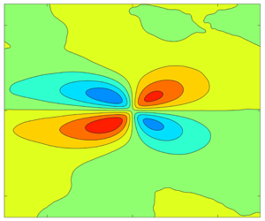
Examples of the correlations of other turbulence quantities are shown in figure 27. Included are contours of $R_{vv}$ and the cross-correlations $R_{uv}$, $R_{\unicode[STIX]{x1D706}u}$, and $R_{\unicode[STIX]{x1D706}v}$ for stations 1, 6, 9 and 12 of case 2. The $R_{vv}$ and $R_{\unicode[STIX]{x1D706}v}$ correlations, which do not involve the streamwise component of the velocity, showed some indication of an increase in spatial extent in the FPG region and a reverse in the ZPG recovery, similar to $R_{uu}$, but the trend was not strong and not consistent between cases. The $R_{vv}$ contours do not exhibit an inclination with respect to the wall, in contrast to $R_{uu}$. The $R_{\unicode[STIX]{x1D706}v}$ contours can be associated with the head of a hairpin vortex (prograde swirl) at the centre of the correlation. Fluid is pulled away from the wall on the upstream side and directed toward the wall on the downstream side. One noticeable effect of the pressure gradient on $R_{\unicode[STIX]{x1D706}v}$ is the larger extent of the negatively correlated region upstream and below the correlation point in the FPG. This would suggest a greater impact of ejections (Q2) related to sweeps (Q4) in the FPG, in agreement with the quadrant analysis results shown above.

Figure 27.

Contours of correlations for case 2, (a) $R_{vv}$, innermost contour $R_{vv}=0.8$, contour spacing 0.2, (b) $R_{uv}$, innermost contour $R_{uv}=-0.45$, contour spacing 0.1, (c) $R_{\unicode[STIX]{x1D706}u}$, outermost contours $R_{\unicode[STIX]{x1D706}u}=\pm 0.015$, contour spacing 0.04, (d) $R_{\unicode[STIX]{x1D706}v}$, outermost contours $R_{\unicode[STIX]{x1D706}v}=\pm 0.01$, contour spacing 0.04.

The trends with pressure gradient were clearer for $R_{uv}$ and $R_{\unicode[STIX]{x1D706}u}$, which do involve $u^{\prime }$. The $R_{uv}$ contours were inclined at a negative angle with respect to the wall, as might be expected for Q2 and Q4 events. The angle, $\unicode[STIX]{x1D703}_{uv}$ was quantified using a least squares fit to define a line though the upstream and downstream points farthest from the centre of the correlation on the $-0.3$ and $-0.35$ contours, and is shown in figure 28 in the coordinates of figure 25. Similar to $R_{uu}$, the magnitude of the inclination angle was reduced in the FPG, starting from an initial value of about $-36^{\circ }$ and approaching an equilibrium of about $-22^{\circ }$ at $(x-x_{f})/L=0.25$ in case 1. Although there is scatter in the results, the trend is the same for all cases and the change in angle is lower for the weaker $K$ cases. The FPG was followed by a return to the ZPG value of approximately $-36^{\circ }$ by the end of the recovery region, and a slight additional increase in magnitude in the APG. The streamwise extent of the correlation, $Lx_{uv}$, was defined as the distance between the most upstream and downstream points on the $R_{uv}=-0.3$ contour. It also followed the behaviour of $R_{uu}$, increasing in the FPG, dropping back to the original value in the recovery, and dropping slightly more in the APG. The percentage change in the length and the streamwise distance in which it occurred were essentially the same as shown for $\unicode[STIX]{x1D703}_{uv}$ in figure 28. The wall-normal distance, $Ly_{uv}$, which was also based on the $-0.3$ contour, behaved similarly, but as with $R_{uu}$, the changes were small.

Figure 28.

Average inclination angle of $R_{uv}$ contours, (a) FPG St. 1–6, (b) ZPG St. 6–9, (c) APG St. 9–12. Symbols from table 1.

The correlation $R_{\unicode[STIX]{x1D706}u}$, as with $R_{\unicode[STIX]{x1D706}v}$, can be associated with the head of a hairpin vortex. Fluid is directed downstream above the centre of the correlation and upstream below, as shown in the LSE results of figure 22. The changes with pressure gradient are the same as those of $R_{uu}$. The inclination of the line between the positively and negatively correlated region of $R_{\unicode[STIX]{x1D706}u}$ decreases with the FPG, and then increases in the recovery and APG regions. The streamwise extent of the correlation, particularly between the correlation centre and the wall, increases with the FPG and then drops in the following regions. These results again agree with those of figure 22. The APG results are very similar to the equilibrium APG DNS results of Lee & Sung (Reference Lee and Sung2009) and Lee (Reference Lee2017). In particular, they noted the decreased extent of the negative $R_{\unicode[STIX]{x1D706}u}$ contours downstream and below the correlation centre, and attributed it to the increased sweep influence as Q4 became larger relative to Q2.

3.7 Turbulence structure, $x{-}z$ plane

The turbulence structure in the $x{-}z$ plane, as shown in studies such as Volino et al. (Reference Volino, Schultz and Flack2007) and Hutchins et al. (Reference Hutchins, Hambleton and Marusic2005) is characterized by high and low speed streaks. This is illustrated in figure 29, which shows LSE results for station 9 of case 2 at $y/\unicode[STIX]{x1D6FF}=0.4$. Clockwise swirl, in the view of the figure, at any location in the plane was used as the conditioning event. Streamwise, spanwise and time averaging were done among all locations with the same $\unicode[STIX]{x0394}x$ and $\unicode[STIX]{x0394}z$ spacings. The conditioning event can be associated with one leg of a hairpin vortex. Although cane vortices, consisting of only a single leg as opposed to a fully formed hairpin, might be present in the instantaneous flow, in the average that LSE shows, the leg of a hairpin should be accompanied by the opposite leg. This is seen in figure 29 as oppositely rotating vortices spaced at about $\unicode[STIX]{x0394}z/\unicode[STIX]{x1D6FF}=\pm 0.5$ from the conditioning vortex at the centre of the field. Between the vortices are high and low speed streaks of positive and negative $u^{\prime }$ induced by the vortices. These streaks extend the full length of the field of view. All the LSE results in the $x{-}z$ plane were qualitatively similar, but the spanwise spacing of the vortices varied. This spacing is shown as a function of streamwise position for all stations of all cases in figure 30 for planes at $y/\unicode[STIX]{x1D6FF}=0.15$ and 0.4. At $y/\unicode[STIX]{x1D6FF}=0.15$ there is a trend of increased spacing in the FPG and a return to the original ZPG value in the recovery, but with the exception of station 6 in the ramp 1 cases, the changes are small relative to the scatter in the data.

Figure 29.

LSE conditioned on clockwise swirl events at $y/\unicode[STIX]{x1D6FF}=0.4$ for St. 9 of case 2.

Figure 30.

Spacing between vortices identified using LSE in $x{-}z$ plane (as in figure 29), (a) at $y/\unicode[STIX]{x1D6FF}=0.15$, FPG St. 1–6, (b) $y/\unicode[STIX]{x1D6FF}=0.15$, ZPG St. 6–9, (c) $y/\unicode[STIX]{x1D6FF}=0.15$, APG St. 9–12, (d) at $y/\unicode[STIX]{x1D6FF}=0.4$, FPG St. 1–6, (e) $y/\unicode[STIX]{x1D6FF}=0.4$, ZPG St. 6–9, (f) $y/\unicode[STIX]{x1D6FF}=0.4$, APG St. 9–12. Symbols from table 1.

In the APG the decrease in the spacing continues. The vortex spacing is approximately 30 % larger at $y/\unicode[STIX]{x1D6FF}=0.4$ than at $y/\unicode[STIX]{x1D6FF}=0.15$. In agreement with the statistics shown above, the effect of the pressure gradient is stronger farther from the wall, and at $y/\unicode[STIX]{x1D6FF}=0.4$ the changes in the vortex spacing are larger than at $y/\unicode[STIX]{x1D6FF}=0.15$. The vortex spacing nearly doubles in the FPG for the ramp 1 cases and returns to its original value in the recovery. It decreases another 20 % in the APG. Changes are smaller for the ramp 2 and 3 cases, but the trends are the same.

Figure 31.

Contours of correlations for case 2 at $y/\unicode[STIX]{x1D6FF}=0.4$, (a) $R_{uu}$, innermost contour $R_{uu}=0.9$, contour spacing 0.1, (b) $R_{ww}$, same contour levels as for $R_{uu}$, (c) $R_{\unicode[STIX]{x1D706}u}$, contour level is 0 at centre of correlation, contour spacing 0.04, red positive, blue negative, (d) $R_{\unicode[STIX]{x1D706}w}$, same contour levels as for $R_{\unicode[STIX]{x1D706}u}$.

Two-point correlations in the $x{-}z$ plane are defined as

(3.2)$$\begin{eqnarray}R_{AB}=\frac{\overline{A(x,z)B(x+\unicode[STIX]{x0394}x,z+\unicode[STIX]{x0394}z)}}{\unicode[STIX]{x1D70E}_{A}\unicode[STIX]{x1D70E}_{B}},\end{eqnarray}$$

where $A$ and $B$ are the quantities of interest at two locations separated by $\unicode[STIX]{x0394}x$ and $\unicode[STIX]{x0394}z$, and $\unicode[STIX]{x1D70E}_{A}$ and $\unicode[STIX]{x1D70E}_{B}$ are the standard deviations of $A$ and $B$ based on data in the full measurement plane for the 1000 vector fields acquired. Streamwise, spanwise and time averaging were done for all location pairs with the same $\unicode[STIX]{x0394}x$ and $\unicode[STIX]{x0394}z$. Contours of the correlations $R_{uu}$, $R_{ww}$, $R_{\unicode[STIX]{x1D706}u}$ and $R_{\unicode[STIX]{x1D706}w}$ are shown in figure 31 for stations 1, 6, 9 and 12 of case 2 at $y/\unicode[STIX]{x1D6FF}=0.4$. In the FPG region, the correlated regions of all quantities increase in size relative to $\unicode[STIX]{x1D6FF}$ in both the streamwise and spanwise directions. In the recovery region, there is a rapid return to the original size. Little change is seen in the APG region, indicating that the structures are growing proportionally with $\unicode[STIX]{x1D6FF}$. The changes are illustrated with cuts through the correlation contours. Streamwise cuts through the centre of the $R_{uu}$ correlation provide the same information and match the results from the $x{-}y$ plane measurements in figure 24. Spanwise cuts are shown in figure 32, showing negatively correlated regions that correspond to the oppositely signed $u^{\prime }$ streaks, on either side of the central peak. If the scale of the figure were increased, additional alternating positive and negative peaks would appear at larger $\unicode[STIX]{x0394}z/\unicode[STIX]{x1D6FF}$. This is shown in the $R_{\unicode[STIX]{x1D706}u}$ contours of figure 31, which include as many as 8 low magnitude streamwise streaks of alternating sign extending across the entire measurement span. A spanwise length scale, $Lz_{uu}$, can be defined based on a particular contour or the distance from the central peak to the nearest negative peak. This was done for all cases, and the results were virtually identical to those of figure 30, since the LSE results and $R_{uu}$ are based on the same data.

Figure 32.

Spanwise slices through self-correlation point of $R_{uu}$ of case 2, (a) centred at $y/\unicode[STIX]{x1D6FF}=0.15$, St. 1–6, (b) $y/\unicode[STIX]{x1D6FF}=0.15$, St. 6–9, (c) $y/\unicode[STIX]{x1D6FF}=0.15$, St. 9–12, (d) $y/\unicode[STIX]{x1D6FF}=0.4$, St. 1–6, (e) $y/\unicode[STIX]{x1D6FF}=0.4$, St. 6–9, (f) $y/\unicode[STIX]{x1D6FF}=0.4$, St. 9–12. Symbols from table 2.

Figure 33.

Contours of $R_{uw}$ correlation for case 2, (a) $y/\unicode[STIX]{x1D6FF}=0.15$, (b) $y/\unicode[STIX]{x1D6FF}=0.4$. Contour level is 0 at centre of correlation, contour spacing 0.04, red positive, blue negative.

The $R_{ww}$ correlation generally followed the same trends as $R_{uu}$, but like $R_{vv}$ in the $x{-}y$ plane, the changes were small relative to the scatter in the results. Contours of the $R_{uw}$ correlation are shown in figure 33. The same contour pattern was shown for ZPG boundary layers in Volino et al. (Reference Volino, Schultz and Flack2007). The four peaks around the centre of the correlation correspond to the expected signs for $u^{\prime }$ and $w^{\prime }$ induced by the counter rotating hairpin vortex legs driving and on either side of a high or low speed streak. The structures increase in size in both the spanwise and streamwise directions in response to the FPG. This is followed by a rapid reversal in the recovery region and little change in the APG. The shape of the contours is different at $y/\unicode[STIX]{x1D6FF}=0.15$ and 0.4. As noted by Ganapathisubramani, Longmire & Marusic (Reference Ganapathisubramani, Longmire and Marusic2006), this may be due to a different inclination angle of the vortex legs at different distances from the wall. Closer to the wall where the inclination angle is presumably smaller, there is more asymmetry between the upstream and downstream sides of the correlation. Farther from the wall, where the leg is presumably more vertical, there is more symmetry. The pressure gradient also has an effect on the asymmetry, and as noted above for the statistics and the structures in the $x{-}y$ plane, the pressure gradient effect is stronger farther from the wall. At $y/\unicode[STIX]{x1D6FF}=0.4$ in the FPG region, the peaks become more elongated in the streamwise direction on the upstream side of the correlation centre, while the peaks expand more equally in the streamwise and spanwise directions on the downstream side. The acceleration was shown above in figures 22, 23, 25 and 28 to reduce the inclination angle of structures with respect to the wall. A reduction of the average inclination angle of the hairpin legs may be responsible for the asymmetry in the same way the asymmetry at $y/\unicode[STIX]{x1D6FF}=0.15$ was attributed to a lower angle. A reduction in the inclination angle of the hairpin and the accompanying elongation in the streamwise direction is consistent with the increasing streamwise scales of all quantities in the near-wall region in response to the FPG. The opposite is observed in the APG, where the streamwise symmetry increases. This is presumably due to the increased inclination angle observed in figure 25(c). The change is subtle, but was seen consistently in the ramp 1 and 2 cases. For the weaker pressure gradient of ramp 3, less change in the structure occurred. The locations of the peak magnitude in $R_{uw}$ in each direction from the centre of the correlation are shown for all stations of case 2 in figure 34. At $y/\unicode[STIX]{x1D6FF}=0.15$ there is no clear progression of the peaks in the streamwise direction, and the changes in the location are relatively small. This indicates that the size of the structure scales with $\unicode[STIX]{x1D6FF}$. At $y/\unicode[STIX]{x1D6FF}=0.4$ there is a clear progression away from the centre of the correlation in the FPG in both the streamwise and spanwise directions, with the streamwise increase noticeably larger than the spanwise. In the ZPG recovery, there is a rapid reversal of the growth and no distinguishable further change in the APG.

Figure 34.

Location of peak magnitude of $R_{uw}$ in each quadrant of $x{-}z$ plane for case 2. Numbers plotted indicate streamwise station number. Red indicates $y/\unicode[STIX]{x1D6FF}=0.15$, black $y/\unicode[STIX]{x1D6FF}=0.4$.