

1 INTRODUCTION
Timbre – A catch-all term for all aspects of a sound not included in pitch and duration. Of no value to the sound composer! (Wishart Reference Wishart1994: 135)
Sounds are traditionally described by the seemingly obvious terms ‘pitch’ and ‘loudness’, but also by some more ambiguous ones, such as ‘brightness’, ‘roughness’, ‘fullness’ and ‘density’, which are generally grouped under the broad term ‘timbre’. The vagueness of this term has, however, led some composers to deny its utility altogether.
With its clearly multidimensional nature, timbre is indeed notoriously difficult to grasp in a quantifiable way, and sometimes considered one of the ‘last frontiers’ of auditory science (Siedenburg, Jones-Mollerup and McAdams Reference Siedenburg, Jones-Mollerup and McAdams2015). Most research has approached timbre by focusing on the perceptual and/or the acoustical properties of isolated short sounds. While obviously linked, few studies have looked at timbre from a musician’s/composer’s perspective (Berger and Fales Reference Berger and Fales2010; Seago, Holland and Mulholland Reference Seago, Holland and Mulholland2010), or used an approach that could make more sense in a musical context. Multidimensional scaling and other perceptual approaches have provided valuable insight into the nature of timbre for the field of psychoacoustics. We aim to add to this knowledge from a more music practice-driven context. In a musical/compositional setting, it is understandably rare (if not impossible) to notate or create directly with a perception or audio-analysis based system. This study aims to approach timbre with methods and tools that are available to practitioners of music. A practitioner might choose to adopt a simplified version of our experimental procedure as part of the development of a set of sonic motives for a work, or of the transitions within it.
1.1 Study motivation
This study examines how timbre changes that are based on physical properties of instrument behaviour or common practices of sound production affect the perception of sonic events. Traditional approaches have usually focused on simple pairs of rather short sound stimuli, presented in succession, separated by (sometimes not further specified) sound gaps (Caclin, McAdams, Smith and Winsberg Reference Caclin, McAdams, Smith and Winsberg2005; Marozeau and de Cheveigné Reference Marozeau and de Cheveigne2007; Siedenburg et al. Reference Siedenburg, Jones-Mollerup and McAdams2015). However, from a compositional standpoint, questions about perceived changes in sounds with no intervening silence (gap-free sounds) are at least as important (Olsen, Dean and Leung Reference Olsen, Dean and Leung2016). Indeed, most musical phrases consist primarily of gap-free sound, with gaps only indicating the beginning and end of a phrase. Even such ‘gaps’ and longer pauses in the event sequences in musical pieces often still contain reverberation, room-sound, ringing acoustic elements (cymbals, guitar feedback), time effects (delay), amplifier noise and so forth.
An electroacoustic/electronic music composer is also concerned that timbral changes in gap-free sounds are not necessarily instantaneous, but rather the sound may morph from one state to another. With the rise of modern Electronic Dance Music (EDM, e.g., Dubstep, Trap, Drum and Bass; Reynolds Reference Reynolds2013) and production techniques, this is probably more often the case than not. EDM often features a continuous dominant bass sound, where the rhythmic structure does not necessarily depend on changes in fundamental frequency (or pitch) of the bass line but on timbre changes. These bass rhythms tend to stay fairly constant in amplitude continuously throughout the whole ‘drop’ – high energy sections of an EDM track that follow ‘rise’ sections, which build tension/anticipation (Solberg Reference Solberg2014). Their main dynamic is usually evoked by sets of automated timbral manipulators such as notch-/bandpass-/peak-filters, phasers, wavetable-modulations, distortions, de-tunings and several others not primarily focused on fundamental frequency (F1) or amplitude. Critics of the genres have even come up with a phonetic approximations of these manipulations, claiming they are only defined by their ‘wub wub’ and ‘yip yip’s, a phonetic approximation of some of the core synthesiser instrument sounds in an EDM song (Beardyman 2011). The perception of these timbral sequences might also be influenced by the common practice of playing such a bass sound alongside other discontinuous rhythmic sounds.
Assuming that for a change in sound to be noticed an acoustic event has to have taken place, the series of experiments described here assessed how much each of the chosen timbre manipulators (which are detailed in Section 3.3) has to be changed for a participant to notice a new event in a gap-free sound stimulus. An event in this context is here defined to be: a segment of time at a given location that is conceived by an observer to have a beginning and an end (Olsen et al. Reference Olsen, Dean and Leung2016; Zacks, Speer, Swallow, Braver and Reynolds Reference Zacks, Speer, Swallow, Braver and Reynolds2007). In a second experiment, we also investigated whether such events can be perceived when the stimuli are gradually transformed from one into another. The transformation approach we used was an entirely practical one, the linear change of the controlled acoustic generator parameter from start-value to end-value over a set time interval.
2 BACKGROUND
2.1 Perceptual measurements
One of the most common ways to describe perception of timbre is by multidimensional scaling (MDS) of timbre spaces, as measured with dissimilarity ratings among short, isolated tones equalised for pitch, loudness and perceived duration (Caclin et al. Reference Caclin, McAdams, Smith and Winsberg2005; McAdams, Winsberg, Donnadieu, De Soete and Krimphoff Reference McAdams, Winsberg, Donnadieu, De Soete and Krimphoff1995; Wessel Reference Wessel1979). The advantage of MDS is that it makes no assumptions regarding the underlying acoustical dimensions. In such a study, listeners only rate the dissimilarity between the members of all possible pairs of sounds from a set of stimuli. The resulting dissimilarity matrices are subjected to multidimensional scaling (Caclin et al. Reference Caclin, McAdams, Smith and Winsberg2005). Dissimilarity rating methods are, however, known to be subject to judgement bias, that is, listeners may only focus on a limited number of acoustic features that they implicitly interpret as reflecting perceptual salience of the parameters. The focused feature (e.g., fundamental frequency, F1) may have such high saliency that for many subjects, no other dimension influences the judgement (Miller Reference Miller1975). Given the multiplicity of acoustic parameters that could be proposed to explain perceptual dimensions, one can never be sure that the selected parameters do not merely covary with the true underlying parameters, as also implied by principal component decompositions of such data. This is especially true for three-dimensional or four-dimensional spaces, where for some dimensions only weak correlations between perceptual and acoustical dimensions are found (Caclin et al. Reference Caclin, McAdams, Smith and Winsberg2005).
Other studies, exploring detectability of change for spectral shape, used two-alternative, forced-choice procedures, often with an adaptive two-down, one-up rule in a staircase scenario, which is similar to our experimental design (Bernstein, Richards and Green Reference Bernstein, Richards and Green1987; Grey Reference Grey1978; Versfeld and Houtsma Reference Versfeld and Houtsma1991). But, as mentioned before, these studies tended to use pairs of rather short stimuli, presented in succession, rather than a change in spectral shape in a continuous sound.
2.2 Timbre descriptors from audio analysis
With the goal of having a more systematic and more measurable approach to direct sound analysis, researchers from the field of music information retrieval (MIR) have also tried to derive reliable, perceptually relevant timbre parameters from audio signals (Peeters, Giordano, Susini, Misdariis and McAdams Reference Peeters, Giordano, Susini, Misdariis and McAdams2011).
It has been described as the holy grail of timbre studies to uncover the number and nature of the MDS dimensions and descriptors (Caclin et al. Reference Caclin, McAdams, Smith and Winsberg2005). Systematic approaches have tried to explain the perceptual dimensions of a given timbre space by correlating acoustic parameters with perceptual dimensions (Iverson and Krumhansl Reference Iverson and Krumhansl1993; Siedenburg, Fujinaga and McAdams Reference Siedenburg, Fujinaga and McAdams2016), still usually using short and isolated tones. Previous studies have often identified the spectral centroid (SC), the logarithm of attack time (LAT) and, to a lesser extent, spectral flux (SFX) as the most salient correlates of timbre space dimensions (McAdams Reference McAdams1999; McAdams et al. Reference McAdams, Winsberg, Donnadieu, De Soete and Krimphoff1995). In continuous perceptions of change in music (where features such as intensity and pitch are highly variable), the factors which best model the perceptions are acoustic intensity and other acoustic aspects of timbre, such as spectral flatness, spectral centroid, spectral flux, spectral spread, inharmonicity and roughness (Olsen et al. Reference Olsen, Dean and Leung2016; Olsen, Dean, Stevens and Bailes Reference Olsen, Dean, Stevens and Bailes2015).
The SC represents the spectral centre of gravity; it is calculated as the weighted mean of the frequencies present in the signal, determined using a Fourier transform, with their magnitudes as the weights. LAT is a descriptor computed using the energy envelope of the signal. It is the logarithm of time from the estimated start and end of the attack. SFX is a time-varying descriptor computed as the amount of variation of the spectrum over time, using pairs of successive Fourier representations of the audio signal.
Overall, available data do not exclude the possibility that there may be acoustic dimensions that only become salient when these identified dimensions (SC, LAT, SFX) are controlled for, which are therefore not revealed as (global) latent dimensions by the MDS approach so far. In particular it has been noted that the spectro-temporal nature of SFX might need to be made more context-dependent to optimise results, as the type of spectro-temporal information that listeners can use in dissimilarity ratings remains unclear and warrants further testing (Caclin et al. Reference Caclin, McAdams, Smith and Winsberg2005).
This project uses gap-free stimuli of constant and normalised amplitude, so temporal parameters, including energy envelope descriptors such as log-attack-time and attack-slope are excluded from the analysis, as they are essentially inapplicable. Also, all the stimuli are static in nature, so spectro-temporal parameters are static for most of the stimuli, except for distorted inharmonic ones which, as discussed in Peeters et al. (Reference Peeters, Giordano, Susini, Misdariis and McAdams2011), are dynamic.
Given our general approach, focusing on the operations accessible to musicians, composers, sound-engineers etc., and the analytical acoustics tools we will use, we now describe the means of production of our sonic stimuli.
3 STIMULI
3.1 Stimulus generation
To generate the stimuli, a new synthesiser was programmed by the first author in the Max 7 (https://cycling74.com) environment. This synthesiser was built in an additive fashion, meaning every partial of the sound had its own sinusoid-oscillator. To be able to represent the entire spectrum a perfectly harmonic (meaning every spectral peak/partial is centred on an integer multiple of F1), complex sound with fundamental frequency of 80 Hz, in the perceivable spectrum from 20 Hz to 20000 Hz, the synthesiser needed 250 oscillators (highest partial 250 times 80 Hz=20,000 Hz); for good measure we used 275. To avoid aliasing artefacts, every oscillator with a frequency higher than 22.05 kHz (due to sounds with F1 higher than 80 Hz) was muted. Every oscillator was manipulable in terms of its frequency and amplitude. The synthesiser is freely available upon request. To prevent the participant from learning a constant temporal point at which the change occurs, the continuous sounds (comprising two successive components, each with an original duration of 1.5 seconds) were played from a random point within the first 500 ms of the sound file. This way the overall sequence-length ranged from 2.5s to 3.0s and the change point correspondingly.
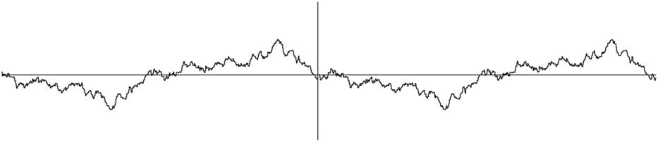
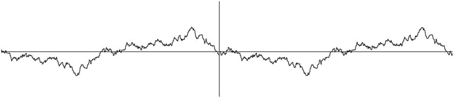
After the sounds for experiment 1 were rendered out (44.1 kHz 16bit, lossless .wav file), they were normalised, using a custom Matlab 2014 routine, to matching RMS (root-mean-square) values. To create the sound sequences of two sounds, and to avoid clicks at their transition, the sounds were connected at zero-crossings and matching wave-shape-positions via the digital audio workstation Cubase 8 (Figure 1).
Illustration of sound connected at a zero-crossing at the corresponding point in the repeating wave form – the left section of this waveform is connected to the right section of the waveform at their common zero-crossing, which is on the vertical line. (Cubase 8 screenshot, Y=Amplitude, X=Time)
To generate the gradual change for all timbre manipulation types between the sounds for experiment 2, the sound sequences were rendered as a whole, instead of as separate sounds such as in experiment 1. For these gradually changing sound-sequences a Matlab 2014 script was created, which calculated the RMS, normalised both parts of the stimulus and implemented a linear amplitude-cross-fade for the morphing section in between, to compensate for any changes in amplitude introduced by the timbre transformation itself. This amplitude-fade was matched to the length of the transition time. Since the RMS is not frequency-weighted, the resulting normalisation applies equally to all frequency components. The same normalisation method was used for all manipulation methods, independent of the type of manipulation.
3.2 Effects of phase
Due to the nature of inharmonic complex stimuli, the phases of the partials do not stay in synchrony. Harmonic complex tones with partials in phase-synchrony, sound distinctly different to those with partials in random phases (Laitinen, Disch and Pulkki Reference Laitinen, Disch and Pulkki2013). As we had reason to expect such phase desynchronisation for at least all of our inharmonic sounds, we selected a replicable set of five different phase starting points for all the partials of all the stimuli, to have partial phases consistently in non-synchrony.
3.3 Timbre manipulations
The fundamental frequency F1 and the acoustic intensity (RMS) were kept constant, so the manipulated parameters were purely timbral. Each manipulation was generated at three different fundamental frequencies that could generally be described as low, medium and high in terms of instrumental ranges or of the range from vocal bass to a still comfortable vocal soprano. Although not directly corresponding to actual notes in the conventional standard tuning pitches, the fundamental frequencies were set at 80 Hz, 240 Hz and 600 Hz respectively, which roughly correspond to E2, B3 and D5, so they were about one and a half octaves apart from their neighbour(s). Motivation for the selected manipulations is discussed in section 3.4. The mathematical formulations of the manipulations are as follows.
3.3.1 Slope manipulation
The amplitudes of partials are varied by a spectral ‘slope’ manipulator α, which is used as the independent variable in experiments,
 $${\rm A}_{k} {\equals}{1 \over {{\rm k}^{{\rm \alpha }} }}$$
where A is the amplitude of the partial of order k=Fk/F1. If α=1, the partials have an amplitude proportional to the inverse of their harmonic number (1, 1/2, 1/3, 1/4, etc.) approximating a sawtooth oscillation; if α=0, all partials and F1 have equal amplitude, approximating a pulse stream. A continuous change of α from 1 to 0 would therefore have all partials continuously rise in amplitude until they are equal in amplitude to F1. This manipulation is closely related to the spectral slope audio descriptor and its linearly correlated spectral centroid audio descriptor (Peeters et al. Reference Peeters, Giordano, Susini, Misdariis and McAdams2011), which was described in Section 2.2.
3.3.2 Odd to even ratio (OER) manipulation
A second manipulation changes partial amplitudes, based on their harmonic number, by multiplying the amplitudes of even-number partials by the OER manipulator β. If perfectly harmonic partials were in phase synchrony, with a slope-value of α=1 and the multiplier for even harmonics set to β=0, the resulting sound would have no even-number harmonics and would approximate a square-wave oscillation; a similar sound but with the multiplier set to β=1 would approximate a sawtooth oscillation. This manipulator would obviously be most closely related to the OER audio descriptor from the audio analysis (Peeters et al. Reference Peeters, Giordano, Susini, Misdariis and McAdams2011).
3.3.3 Pluck manipulation or comb-filter shaping
A third manipulation method is based on the normalised absolute sine-function,
 $${\rm A}_{k} {\equals}{{\left| {\sin \left( {\pi \gamma k} \right)} \right|} \over {\sin \left( {\pi \gamma } \right)}}$$
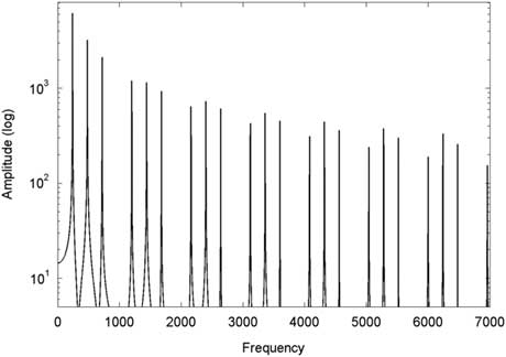
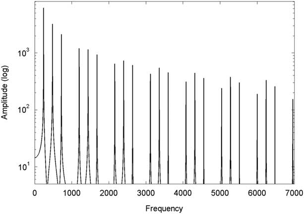
with partial amplitude A for the kth harmonic, where the pluck manipulator γ changes which harmonics are attenuated or silenced (see Figure 2). The value for γ ranges between 0 and 1. If the value is set to 1/2, every second partial would be reduced to zero. If it was 1/3, every third partial would be reduced to zero, etc. More precisely, the absolute sine-function shapes the amplitude spectrum with a spectral envelope resembling a comb filter, the combs’ spikes representing the zeroed spectral positions. This manipulation does not have a particular corresponding audio descriptor, but would most likely affect multiple ones to varying degrees (SC, OER, spectral flatness, etc.)
Illustration of frequency spectrum for γ=.25, F1=240 Hz.
3.3.4 Inharmonicity manipulation
The inharmonicity manipulator affects the frequency of the partials, based on the formula
 $$F_{{\left( k \right)}} {\equals}F_{{\left( {k{\minus}1} \right)}} {\plus}F_{1} \delta ^{k} $$
where k is the index of the harmonic, and δ is the constant by which the ratio of harmonics is stretched or compressed. Values for δ>1 result in stretched partials, δ<1 in compressed partials. When δ=1, the result is a perfectly harmonic sound. This manipulation would be most accurately captured with the inharmonicity audio descriptor from the audio analysis (Peeters et al. Reference Peeters, Giordano, Susini, Misdariis and McAdams2011).
3.3.5 Distortion manipulation
Lastly, and perhaps most importantly, distortion of the signal will be another variable, provided by digitally clipping the signal at fixed amplitude. For distortion, the normalised source signal amplitude is being multiplied by seven and afterwards every value greater than +1 is set to 1 and every signal smaller than -1 is set to -1. This particular multiplication (or ‘gain’) value has been chosen because it provides a prominent and unmistakable distortion effect. The effect is usually the result of increasing signal amplitude gain past the maximum capacity of any given sound system or amplifier (often referred to as ‘overdrive’). In digital systems overdrive/distortion corresponds to ‘clipping’ of the signal, which is why, within the Max/MSP 7 environment, the ‘clip’ object was used in the signal chain to bring the signal back to ±1 so as to achieve the desired effect. Similar to the pluck manipulation, this manipulation does not have a particular corresponding audio descriptor, but would most likely affect multiple ones to varying degrees (SFX, SC, spectral flatness, inharmonicity, spectral slope etc.).
3.4 RELATIONS OF TIMBRE MANIPULATORS TO PHYSICAL CONCEPTS IN MUSIC GENERATION
All the manipulation conditions relate to a physical concept of music creation, performance or production, as used in electroacoustic music, rock/pop, contemporary classical, or almost any other form of music.
3.4.1 Slope manipulation
It is well known that the amplitudes of upper partials increase more than those for lower partials when instruments are played with a higher intensity, which makes them sound brighter (Dannenberg and Derenyi Reference Dannenberg and Derenyi1998). In conventional synthesisers, this often leads to the velocity of the input being linked not only to the overall amplitude, but also to the frequency of a cut-off filter (low-pass), to imitate the behaviour of physical instruments.
3.4.2 OER manipulation
The ratio of odd to even number harmonics has been a primary manipulator in synthesisers since the first Moogs in the 1960s and 1970s, where crossfading of multiple oscillators allowed for smooth variation between oscillation shapes (Moog Reference Moog1977). The most common oscillation shapes in subtractive synthesis are still the sawtooth- and the square-wave, whose defining difference is the absence of even harmonics in the square-wave as opposed to the sawtooth-wave, which contains all the multiples of F1. Square-waves are also closely associated with the concept of fundamental audio distortion/overdrive, which primarily adds odd harmonics. With increasing levels of overdrive- or distortion-gain, a pure sine-wave transforms into a square-wave by introducing, and then continuously increasing, odd number harmonics of F1. When there is complete attenuation of even number harmonics this can also be seen as a special case of the pluck manipulation set to
 ${\raise0.5ex\hbox{$\scriptstyle 1$}\kern-0.1em/\kern-0.15em\lower0.25ex\hbox{$\scriptstyle 2$}}$
; however, the OER manipulation varies the amount of attenuation, whereas the pluck-function varies the attenuation position along the frequency axis.
3.4.3 Pluck manipulation
With string instruments like a guitar, the position where the string is plucked in relation to the bridge and the nut or the finger-stop point (the two suspension points of the string) has a noticeable impact on its sound. Plucking a string close to the bridge results in a brighter sound, whereas plucking closer to the fingerboard or the midpoint of the string results in a tone mellower and less rich in high frequency components. In ideal cases, the harmonics with nodes on the plucking position should be attenuated so, assuming an ideal string, a note plucked at 1/5 of the string-length will lack all harmonics that are a multiple of five. The most drastic attenuation of harmonics is achieved by plucking at the middle point of the string, which mutes every even order harmonic, resulting in a wave approximating a square wave. Mathematically we realise this by modifying the sinc (sine cardinal) function as suggested in Traube and Smith (Reference Traube and Smith2001).
3.4.4 Inharmonicity manipulator
Many instruments exhibit imperfectly harmonic structures. Most obviously many percussion instruments, in particular bells, feature large amounts of distinctly inharmonic partials and when it comes to computer-music, there is no physical limit to the extent of partial detuning. But also pitched instruments like the piano are often characterised by the slightly detuned nature of the partials of the hammered strings (Järveläinen, Välimäki and Karjalainen Reference Järveläinen, Välimäki and Karjalainen1999; Schuck Reference Schuck1943), particularly the bass strings. The same goes for groups of instruments playing in unison in an orchestra or big band setting (Cohen Reference Cohen1984). The inharmonicity manipulator serves as a general representation of this characteristic, which stretches the partials evenly along the whole spectrum by an exponential value. With the implemented manipulation, the distance between partials i and i+1, is the distance between partials i-1 and i, multiplied by constant δ.
3.4.5 Distortion
Whole genres of music are defined to a large extent by the nature of the distortion of the sounds (e.g., Djent, Drone-Doom, Noise, Glitch) (Berger and Fales Reference Berger and Fales2010; Van Nort Reference Van Nort2006). The literature so far usually notes distortion simply as an effect, adding (mostly odd) harmonics to a given signal. Given that distortion/saturation/overdrive effects are among the most popular not only within guitar-driven but also electronic and experimental music as well as in studio production (tape saturation, microphone preamp overdrive, tube compressors, etc.), it seems to be a manipulation worth investigating. Its effect is completely dependent on the input signal, often accentuating the signal’s properties.
Applying distortion to a perfectly harmonic sound will tend to make the sound brighter and increase amplitude of odd harmonics hence will be correlated with the slope and OER manipulators. But importantly, if the input has slightly inharmonic partials, which usually is the case, it turns static signals into dynamic ones with the resulting beating between the inharmonic partials of the original sound, and the new partials introduced by the distortion. Distortion is also a natural product of any physical system with a finite amplitude/pressure bandwidth, hence it commonly arises in the real world including the auditory system itself (Lee, Skoe, Kraus and Ashley Reference Lee, Skoe, Kraus and Ashley2009). As detailed in Section 4, for these reasons, we chose to apply distortion, but solely to inharmonic input sounds.
4 EXPERIMENT 1
Experiment 1 sought to identify the perceptual threshold (PT) for musicians in relation to our chosen timbral manipulations. It was also intended that the PT values derived would inform subsequent experiments involving transitions.
4.1 Experimental Setup
The experiment, including the tutorial, was coded in the Max/MSP 7 environment. The participants (n=21, females =11, males=10; musicians=11, non-musicians=10, age 18–68 years) were placed in front of a laptop and given a pair of headphones (AudioTechnica M50x). Musicians were defined as people with at least four years of formal musical training. They would then listen to a succession of sounds, indicating after each if they noticed a change within the sound, or not. To indicate a noticed change, they were asked to press the spacebar; if they did not hear a change in sound, they were asked to press the ‘N’ button. The response would then prompt the next stimulus of a randomly selected manipulation, frequency and starting value to be presented. The answers were recorded on the same laptop presenting the stimuli. Before the recording started, the participant had to finish a short tutorial with 10 stimuli, explaining the setup. Since the tutorial’s aim was also to familiarise the participants with the type of change they were going to identify, the tutorial comprised a number of sounds with a very clear change in timbre, and a number of sounds without any change. In this tutorial, participants were also informed whether or not they had correctly identified a change in timbre. The participants were told that reaction time would be measured as well, but they should prioritise accuracy over speed. After blocks of 50 stimuli, they were treated to either pictures of cute animals, or pictures with hilarious puns (sometimes both) and had the option of taking a small break. The experiment took roughly 50 minutes to complete.
The stimuli were presented to the participants in a staircase approach as now described. The staircase procedure is one of the standard techniques used in psychoacoustics to determine perceptual thresholds. The specific 2 down/1 up method implemented here establishes the size of the change that is correctly identified with a probability of 70.7% (Levitt Reference Levitt1971).
From hereon we often abbreviate ‘manipulation’ as FX (an acronym for ‘effect’ familiar to audio workers) and ‘start value’ as SV (see below). For each given condition (FX-method, SV and F1-frequency), the participant would be presented with the stimulus, representing the average perception threshold of the chosen FX, based on the previous participants. The data for the main experiment was initialised on available data from pilot tests. This average was constantly updated. If a participant responded as not noticing a change within the sound, the amount of timbre-change in the stimulus was increased by one step size (step sizes are defined in the following section). This would be repeated, until the subject noticed the change in timbre. When the participant reported noticing a timbre change, the stimulus would then be repeated once more, and if the change in sound was recognised again, then the timbre change would be reduced by one step size. Whenever the change in timbre would increase so much for the subject to notice it, or to such a small value that it was not noticed anymore, this would trigger a ‘turnaround’ within the staircase. In a turnaround, the direction of the staircases switches from increasing to decreasing or vice versa. The stimuli were presented until four turnarounds were recorded, providing two upper limits and two lower limits of the perception threshold for the participant. The resultant perception threshold measure is the mean of these four turnaround values. To avoid the possibility of the participants learning the staircase, which might influence their ratings, the 45 different component items (
 $5 FX{\times}3 F1{\times}3$
SV) were presented to the subjects in random order. The FX-method, SV and F1 was chosen at random, but the number of steps chosen were dictated by the participants’ earlier responses to the same FX-method, SV and F1. For each trial there was a 10% chance for a dummy trial to be selected. In a dummy trial, a stimulus was played, similar to the regular ones, but without any change in timbre. Using the listeners’ responses to these, false alarm rates were calculated, and participants with false alarm rates higher than 25% were excluded.
The three start values (SV) and step sizes for each manipulation are as follows.
4.1.1 Slope manipulation
• Step size: 0.01
• Start Values:
• α=1 (Sawtooth oscillation) Range α=1.0–1.1 (10 steps)
• α=2 (only the first few harmonics are perceivable and very attenuated, sine-like) Range α=2.0–2.1 (10 steps)
• α=1.5 (midway-point) Range α=1.5–1.6 (10 steps)
4.1.2 OER manipulation
• Step size: 0.03333
• Start Values:
• β=0 (Square wave oscillation) Range β=0.0–0.3333 (10 steps)
• β=0.33333 (10 step sizes distance from first value) Range β=0.3333–0.6666 (10 steps)
• β=0.66667 (10 step sizes distance from β=0.33 and −10 from β=1, which would be a sawtooth) Range β=0.6667–1.0 (10 steps)
4.1.3 Pluck manipulation
• Step size: 0.01
• Start Values:
• γ=.5 (square wave oscillation, every second harmonic is silenced) Range γ=0.5–0.6 (10 steps)
• γ=0.3333 (every third harmonic is attenuated) Range γ=0.3333–0.4333 (10 steps)
• γ=0.25 (every fourth harmonic is attenuated) Range γ=0.25–0.35 (10 steps)
4.1.4 Inharmonicity manipulation
Pilot tests revealed vastly different perceptual sensitivity depending on whether SV for δ was set for a perfectly harmonic sound (δ=1), compared with any sort of inharmonic sound (δ≠1). For this reason two separate scale step sizes were selected, such that the step size for δ=1 is 1/5th the step size for δ≠1. Also since the results occupied a wider range across the different conditions, the range was increased from 10 to 20 steps.
• Step size for start-value of δ=1: 0.0002 Step size for start-value of δ≠1: 0.001
• δ=1 (perfectly harmonic sawtooth) Range δ= 1.0–1.004 (20 steps)
• δ=1.001 (mildly detuned) Range δ=1.001–1.021 (20 steps)
• δ=1.01 (very inharmonic, second partial (F1*2) already far enough from perfect harmonicity, to be potentially perceived as individual note (Moore Reference Moore1986)) Range δ=1.01–1.03 (20 steps)
4.1.5 Distorted inharmonicity
Distortion is a special case. With perfectly harmonic sounds, it increases the amplitude of harmonics in general and odd harmonics in particular. In that way it is fairly similar to the already described slope and OER manipulations. With inharmonic sounds, however, it generates completely new harmonics based on the inharmonic partials of the source sound (at frequencies that are integer combinations of the frequencies in the original sound, such as combination and difference tones). With that in mind, it made sense to repeat the inharmonicity manipulation staircase, but with an applied fixed distortion, which first multiplied the overall amplitude of the signal by seven, and clipped the resulting amplitude at the fixed value of 0.7. These values were chosen to have a very obviously audible distortion effect. The other values are identical to the ones from the inharmonicity manipulation, except for the step sizes.
• Step size for start-values for δ=1: 0.000005 Step size for start-values for δ≠1: 0.001
• δ=1 (perfectly harmonic sawtooth) Range δ=1.0–1.0001 (20 steps)
• δ=1.001 (mildly detuned) Range δ=1.001–1.021 (20 steps)
• δ=1.01 (very detuned, first partial already far enough from perfect harmonicity, to be potentially perceived as individual note) Range δ=1.01–1.03 (20 steps)
Since the discrepancy in pilot responses between harmonic and detuned SVs was even more pronounced for the distorted inharmonicity condition, the step size for δ=1 is 1/200th the step size for δ≠1.
4.2 Data analysis
As the distribution is skewed (PT is a non-negative number), the 95% confidence intervals were calculated with the bootstrap method in Matlab 2014. The range of the staircases are 10 steps for the slope, OER and pluck conditions, and 20 steps for both of the inharmonic conditions. If a participant went out of bounds in the staircase, the PT was substituted with a value one bigger than the staircase range (21 for inharmonic ones, 11 for the others). If the participant hit the floor, where there was zero step size change, and still reported a noticed change in timbre, the result was discarded as a false alarm, as zero step size constitutes no physical change.
To model the influence of the variables, we used a Bayesian linear mixed effects model (a weakly informative student t-distribution prior, three degrees of freedom, centred at zero, was applied to all population-level effects) with the brms package (Bürkner Reference Bürkner2016) of the R statistics software (version 3.5.0). The perception threshold was defined as the response variable, SV, F1-frequency and musician status as population-level effects, SV and F1-frequency as group-level effects, grouped over subject (these are analogous to the fixed and random effects used in a classical, non-Bayesian statistical framework). To be a more musical representation of pitch, the F1-frequency was converted to
 $12\log _{2} {{F_{1} } \over {F_{{{\rm ref}}} }}$
. This way each unit represents a semitone, with
 $F_{{{\rm ref}}} $
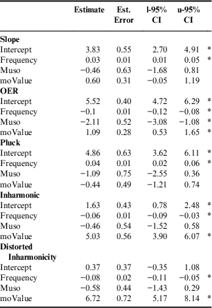
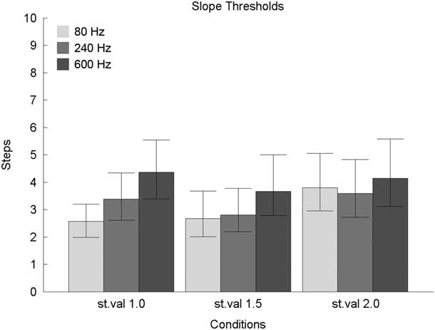
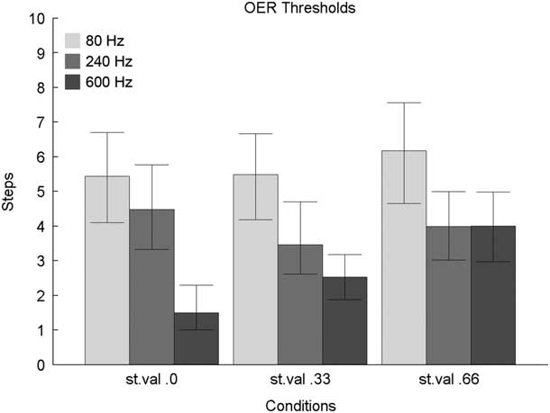
being 80 Hz (lowest F1 value) so F1 in this context refers to the converted frequency. Since SVs are not necessarily linearly spaced and may not have a linear impact on PT, brms allows for the SV factors to be treated as monotonic values, meaning they are separate factors, but in an ascending (or descending) order. The effects were calculated for each block of FX-type separately, as the values hiding behind SV are fundamentally different for each FX-type, and F1-frequency does seem to have varying impact on the PTs depending on FX-type (as seen in Figures 3–8). The regression coefficients (b), standard errors (SE) and upper and lower 95% confidence intervals are reported for F1-frequency, musician status and monotonic SV effects in Table 1.
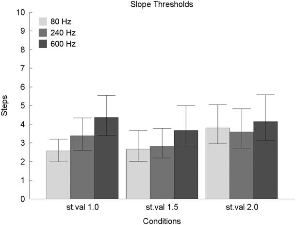
Mean PT for ‘Slope’ FX.
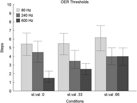
Mean PT for ‘OER’ FX.
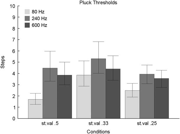
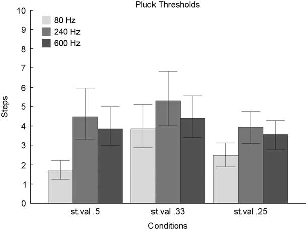
Mean PT for ‘Pluck’ FX.
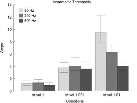
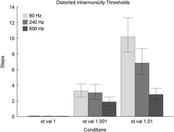
Mean PT for ‘Inharmonic’ FX.

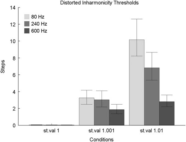
Mean PT for ‘Distortion IH’ FX.
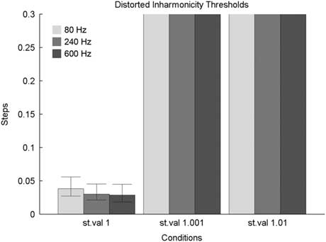
Same as Figure 7 but with different y-range.

Population-level effects

Key: Intercept: PT when everything else would be set to zero, Frequency: F1, Muso: Musicianship, moValue: monotonic start value, l-95% CI: lower 95% confidence interval, u-95% CI: upper 95% confidence interval
Note: The Estimate is the mean of each effect’s posterior distribution, l-95% and u-95% are the lower and upper bounds of the effect’s 95% credibility interval (the data tell us that the effect’s true size has a 95% probability of falling in this interval). If the 95% CI does not cross zero, the effect can be considered ‘significant’ and is marked with a star.
4.3 Results for experiment 1: timbre perception thresholds
The first experiment examined the minimum PT for instantaneous change for each of the proposed conditions, in a 2-up-1-down staircase procedure. The independent variable used is the value of the manipulated parameter; the dependent variable is the measured perception threshold (PT). To see if established differences for just-noticeable differences (JND) in pitch perception between musicians and non-musicians (Tervaniemi, Just, Koelsch, Widmann and Schroger Reference Tervaniemi, Just, Koelsch, Widmann and Schroger2005) also apply to timbre perception, both musicians and non-musicians were tested and musicianship was used as an independent variable.
The results for all participants in experiment 1 are presented in Figures 3–8. The y-axis represents the PT in units of step-sizes according to the specific FX-Type (the step sizes were defined in Section 4.1). The bars are grouped along the x-axis with respect to the specific SV of the FX-type. The different shadings represent the different F1-frequencies for the tested PT.
Monotonic influences of pitch/frequency (F1) can be seen for most manipulations other than pluck, where the effect seems non-monotonic. Clear dependence on SV is apparent for inharmonic and distorted inharmonic FX. These impressions are interrogated by means of separate models for each manipulation. In Table 1 we show solely the parameters of the population level effects, respectively for each manipulation.
The Bayesian linear mixed effects models show that frequency is a significant predictor for all five FX conditions (none of the 95% CI cross the zero value).
The ‘Estimate’ for each predictor is its effect size, which is how much the response variable (PT) changes for each unit change of that predictor (frequency, musicianship, SV), all else being equal. The units of frequency are semitones, musicianship is coded as 0 and 1. The SV (moValue) is set as a monotonic predictor, treating every tested SV as one separate step (the model ascribes the appropriate distinctive step sizes). The ‘l-95% CI’ and ‘u-95% CI’ display the lower and upper range in which the true effect size will fall into with 95% probability and the Est. Error displays the estimated standard error.
As can be seen in Table 1, the coefficient for pluck is diminished by the apparent non-linear nature of the response, which could be assessed fully by further modelling (e.g., by removing the monotonic constraint on the factor levels). The influence of the SVs is significant for both the inharmonic and distorted-inharmonic FX and some of the slope/OER/pluck FX as well.
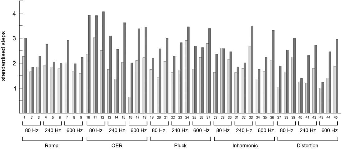
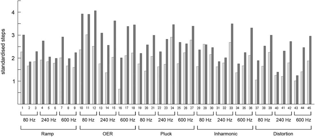
When calculating separate means for musicians and non-musicians and then standardising these over the standard deviation of the corresponding manipulation, we get two separate vectors (each with 45 entries,
 $5{\rm }FX{\times}3{\rm }F1{\times}3{\rm }SV$
), comparing the PT of musicians to non-musicians in units of standard deviation as shown in Figure 9. The Spearman correlation between these two vectors – that is, between musicians and non-musicians – is r=.83. The mean ratio between the standardised non-musicians and musicians PT is 1.35. Since the ratio quantifies PTs of non-musicians over musicians, the >1 value indicates that musicians have smaller PTs and are thus more sensitive in detecting timbral differences. Table 1, however, shows musician status to be significant only for the OER-FX.
All 45 conditions, standardized and split between Musicians (light bars) and Non-Musicians (solid bars). The high correlation between these two populations indicates similar perception patterns for both.
4.4 Experiment 2: effects of transition time
The second experiment is a simple development from the first experiment, providing a transition between the two sounds. The focus of this is to investigate if and how the results of experiment 1 change if the control parameters do not instantly switch from one state to the next. Instead they change linearly over two different time windows, transforming the first sound into the next.
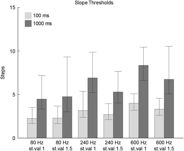
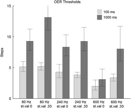
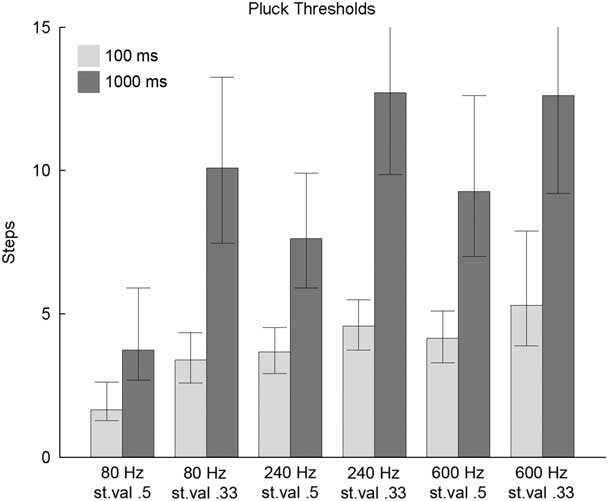
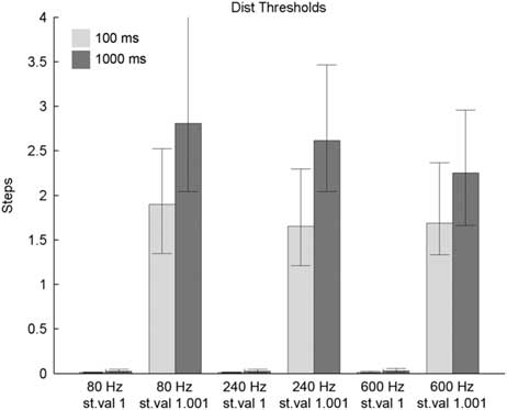
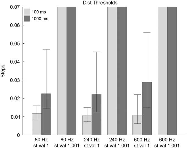
In addition to the previous conditions, a new variable of transition time (TT) was thus introduced, with the two fixed values of either 100 milliseconds, or 1,000 milliseconds. To keep the length of the experiment reasonable (<60 min), the number of SV conditions was reduced (two instead of three), as was the number of FX-types (Inharmonic was discarded, since it is very similar in nature and results to the Distortion FX). Since the responses were similar between musicians and non-musicians in experiment 1, experiment 2 featured only musicians (n=13, 5 female, 8 male). Due to the wide range of PT values, y-axis limits in Figures 10–14 range from 0.07 to 15.
Mean PT for ‘Slope’, TT 100 ms and 1000 ms.

Mean PT for ‘OER’, TT 100 ms and 1000 ms.

Mean PT for ‘Pluck’, TT 100 ms and 1000 ms.

Mean PT for ‘Distorted Inharmonicity’, TT 100 ms and 1000 ms.

Same as Figure 13 but with different y-range.

Figures 10–14 show consistently higher PTs for the 1,000 ms conditions (solid bars) across all FX-types and SVs. This means it is harder to detect change when it occurs more gradually.
Due to this global impact of TT, the PTs were normalised. The PTs were transformed to ratios of their 100 ms values in the Bayesian mixed effects model. This ‘Ratio’ is every PT value expressed in units of the 100 ms PT of its corresponding condition (FX-type, SV, F1), so the original 100 ms PT becomes ‘1’, and the 1,000 ms value becomes the ratio between the 1,000 ms and 100 ms values. This allows us to model the impact of TT globally, rather than for each FX-type separately.
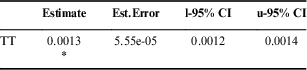
A Bayesian regression model with the new ‘Ratio’ as response variable, TT and the Intercept as population effects and Intercept also as group level effect, grouped over subject (same priors as in experiment 1), shows TT to be significant (Table 2).
Estimating the population-level effect of TT within the Bayesian regression model

Since TT is in milliseconds, the values appear small and close to zero. The coefficient estimate is 0.0013, which is equivalent to an effect size of 1.3 per second. This indicates the ratio between the two sounds increases by 1.3 for each second added to the TT. Or more generally, the PT for transition time of 1,100 ms is 2.3 times as big, as the PT for 100 ms.
With the TT of experiment 2, slightly different loudness compensation was used so the stimuli were not identical in loudness to those in experiment 1. The results are still broadly comparable, and the 100 ms TT had PTs of similar size to those of the instant transition of experiment 1, often even smaller.
5 DISCUSSION
The experiments investigated perception thresholds (PT) for a select number of timbre manipulations (FX). Additionally they established the influence of fundamental frequency (F1), transition time (TT), musicianship and the starting value (SV) of the specific FX. While the range of different FX, F1 and SVs is obviously limited, the results do give an indication of general perceptual behaviour towards these timbre changes. The novel approach, which uses the synthesiser parameters as the dimensions for the PT, unfortunately limits the applicability of the results specifically to the FX used in this experiment and might not generalise over sounds of all sorts. An additional limitation is that PT would have to be established for every timbre manipulation (and all interactions thereof) individually. It does, however, open up the possibility of applying the approach and such results in a context of informed music creation and production, where it may be more intuitive to grasp for musicians than the traditionally used timbre descriptors (SC, SFX, etc.), or the multidimensional timbre spaces of MDS. While it might still make sense for musicians, if told to use a brighter or darker sound – analogous to spectral centroid – most would probably be confused if told to perform with more spectral flatness or higher spectral flux. Referencing their plucking position or specific features of their synthesiser, however, might make more sense to them.
A potentially valuable future approach could be to derive how much change in a parameter would correspond to a doubling or halving of a perceptual quality; for example, render a sound about half as ‘hollow’ by adjusting the OER parameter by a specific/predictable amount. This likely cannot be derived from the current data, but these ideas may inform the future path of similar research.
Some of the results are unsurprising; for example, it seems intuitive that a change in inharmonicity is dramatically easier to perceive when starting from a perfectly harmonic sound, as opposed to a change from an already inharmonic sound to a slightly more inharmonic one. Also it is as expected that musicians tend to notice changes in timbre more readily than non-musicians. The correlation of 0.83 between the performances of the two groups, however, suggests, apart from a generally lower mean PT, musicians and non-musicians behave similarly across the tasks. From the musicians’ point of view, which this study focuses on, this is a rather comforting observation, since it indicates that timbral manipulations done by the musician are perceived in a similar manner by non-musicians. The second experiment confirmed the equally intuitive hypothesis that longer transition times lead to a higher PT. Composers can take systematic note of this, if they wish, in designing their continuous sound sculpting and morphing. The results from the Bayesian regression models show the ratio between PT increasing by approximately 1.33 for a second (1000 ms) added to the transition time. For example, a PT for TT 1,100 ms would be approximately 2.3 times as big, as its 100 ms counterpart. This effect is measured jointly across all tested timbre-FX.
An interesting detail about the different PTs is that, while F1 is consistently a significant influence for the PT within each FX-group, its impact differs between FX-groups. Timbre changes in ‘slope’ are easier to identify for lower F1, but harder for changes in OER and inharmonic/distorted inharmonic, whereas the impact is more complex for pluck.
The pluck results are noteworthy for a couple of different aspects as well. The pluck PTs from experiment 1 suggest a non-linear effect of both F1 and SV. While the regression models show a significant negative impact on the PT (‘negative’ in the sense, that the PT actually goes up), Figures 10–14 clarify that task performance indeed decreases in the steps from F1 80 Hz to F1 240 Hz, but then slightly increases again for F1 600 Hz. Generally, this suggests that different timbral manipulations may be more useful in different pitch ranges.
The same seems to be the case in terms of pluck SVs, where performances for values of 0.5 (every second partial attenuated, square wave) and 0.25 (every 4th partial attenuated) are similar, but the task performance for .33 (every third partial attenuated) is decreased. Interestingly, this non-linear interaction of F1 seems to be turning to a more nearly monotonic one for the second experiment, where TT is introduced. The PT increases for both 100 ms and 1000 ms from 80 Hz to 240 Hz and again from 240 Hz to 600 Hz.
Due to reducing the SVs to two, we unfortunately cannot be sure if the (non-)monotonicity of SV might be impacted for most FX as well. From the authors’ experience of listening repeatedly to these stimuli, we suspect this might be due to a particular feature of the pluck-FX manipulation. The attenuation of specific partials creates very distinct attenuation spikes in the spectrum of the sound. When changing the FX-parameter, these spikes move progressively through the frequency spectrum in a way which is very noticeable. With the transition segment of the sound introduced in experiment 2, the participant now can identify the whole segment of changing sound in between the two fixed timbres, as opposed to just discriminating two different sounds from one another in experiment 1.
Something similar might be happening for the distorted-inharmonic condition, where the impact of F1 is reduced in experiment 2. Additionally, while the task performance for 100 ms is still better than for 1000 ms in distorted-inharmonic, both actually perform on par, or better when compared to no TT from experiment 1. This implies a different impact of the presence of a TT-segment which is itself more detectable on the PT for some conditions (pluck and distorted-inharmonic) than others (slope and OER). In a musicking context, this might suggest that when distinguishing rhythmic patterns in an otherwise more constant sound, it might sometimes be beneficial to have short transition times (<=1 sec or thereabouts) in between sounds, rather than changing them instantly.
The reason for changes in distorted-inharmonicity and pluck being easier to detect than slope or OER with 100 ms transition times instead of abrupt changes, could be a similar one to F1 having different impact on pluck PT with transition times. Slope and OER only affect partials’ amplitudes in a global way, which could also be approximated with a simple crossfade. Pluck and inharmonicity either move distinct spectral features through the spectrum (pluck), or move the partials altogether (inharmonicity).
Another result that is expected, but yet has surprising aspects, is the impact of audio-distortion. When comparing the PTs for SV of 1 between Figure 6 and Figures 7/8, the difference is striking. While it makes sense for changes to be more noticeable due to the phasing and masking effects of the slightly inharmonic partials generated by the distortion versus the ones inherent to the original sound, for the PT to drop by a factor of almost 50 in the case of changes from perfectly harmonic to slightly inharmonic is still remarkable. This sensitivity to timbre changes in sounds that are distorted and almost perfectly harmonic might give an indication as to why distortion as an audio effect remains hugely popular in musicians, music producers and music-listeners, despite not seeming to be a very popular topic among researchers, and suggests ways it may continue to be used effectively.
Acknowledgement
This study was supported by the Western Sydney PRA and IPRS 2016 International Post-Graduate Research Scholarship and Western Sydney Post-Graduate Research Award, held by the first author. We thank Dr Steffen Herff for statistical advice and members of the MARCS Institute Music Cognition and Action Group for helpful comments on earlier drafts.