



1 Introduction
Porous polymer membranes with asymmetric pore structure are usually prepared by interface polymerization or a phase inversion process (Strathmann Reference Strathmann2011). In the latter process, a homogeneous polymer solution is precipitated in a coagulation bath. At contact of the polymer solution and coagulation bath, the solvent diffuses into the coagulation bath while the non-solvent diffuses into the polymer solution. Due to the miscibility gap of the polymer mixture, the polymer solution phase separates into polymer-rich and polymer-lean phases, respectively, forming the matrix and pores of the membrane. Depending on the properties of the components, the composition of the polymer solution and the coagulation bath, as well as process conditions, different morphologies of the membrane are formed.
In the last 50 years, different polymer systems were experimentally and theoretically investigated to identify the mechanism that leads to the formation of different morphologies, e.g. sponge pores or finger pores (Strathmann, Kock & Amar Reference Strathmann, Kock and Amar1975; Koenhen, Mulder & Smolders Reference Koenhen, Mulder and Smolders1977; Kimmerle & Strathmann Reference Kimmerle and Strathmann1990; Boom Reference Boom1992; Smolders et al. Reference Smolders, Reuvers, Boom and Wienk1992; van de Witte et al. Reference van de Witte, Dijkstra, van den Berg and Feijen1996; Yu, Yang & Xiang Reference Yu, Yang and Xiang2014). All postulated theories on the formation of pores in porous polymer membranes are based on liquid–liquid phase separation of the polymer solution followed by solidification of the polymer-rich phase as the main mechanism that leads to a porous structure (van de Witte et al. Reference van de Witte, Dijkstra, van den Berg and Feijen1996). Nowadays, this mechanism is generally accepted to explain the formation of sponge pores. In the literature, theories on the origin and formation of finger pores are more diverse, sometimes contradictory and not well understood, especially at their early stages. For example, Strathmann et al. (Reference Strathmann, Kock and Amar1975) postulated mechanical stress and shrinkage of the polymer-rich phase followed by cracks as the origin of these pores. Matz (Reference Matz1972) and Frommer & Messalem (Reference Frommer and Messalem1973) argued that gradients in the surface tension form convective cells as the origin of finger pores. Reuvers & Smolders (Reference Reuvers and Smolders1987) introduced different de-mixing times (instantaneous/delayed de-mixing) that are responsible for different morphologies. Ren, Li & Wong (Reference Ren, Li and Wong2004) observed viscous fingering, a hydrodynamic instability due to a displacement of a more viscous fluid by a less viscous fluid, and postulated it as the origin of finger pores.
In this article, we focus on viscous fingering phenomena in the early stage of pore formation. This is because viscous fingering is not yet investigated in detail in the context of porous polymer membranes to answer open questions and clarify diversities in available theories. Viscous fingering is a hydrodynamic instability that is observed on different length scales. It arises when a less viscous fluid displaces a more viscous fluid. The phenomenon is observed in miscible as well as in immiscible systems. The main driving force in these systems is the force of displacement by the less viscous fluid. Its origin can be a body force, e.g. gravity, an external pressure gradient or capillary forces in three-phase systems. Its counterpart is dispersion and surface tension in miscible and immiscible systems, respectively. In both cases viscous fingering is typically studied in Hele-Shaw cells (Hele-Shaw Reference Hele-Shaw1898).
In the literature, viscous fingering is typically discussed in the two extreme cases, i.e. miscible and immiscible. Immiscible viscous fingering is studied in the limit of very small diffusive mass transport between two distinguishable phases. In this case, a sharp interface is assumed and only surface tension between two immiscible phases is considered while diffusive mass transfer across the interface is neglected.
Miscible viscous fingering is studied in the limit of very small surface tension between two miscible fluids, where the viscosity depends on the concentration. Here, a wide diffusive interface between adjoint fluids is assumed. Surface tension is neglected and diffusive mass transport across the interface dominates. Both cases are limiting cases of the more general case where surface tension and diffusive mass transport may be present. In the present model we consider diffusive mass transport and capillary stress and, therefore, it covers the general case.
In principle, miscible as well as immiscible viscous fingering may occur during precipitation of polymer membranes depending on the preparation conditions. Regarding to immiscible viscous fingering, it was first analysed in the 1950s by Hill (Reference Hill1952), Saffman & Taylor (Reference Saffman and Taylor1958) and Chuoke, van Meurs & van der Poel (Reference Chuoke, van Meurs and van der Poel1959). Since then, further investigations were followed by Bensimon et al. (Reference Bensimon, Kadanoff, Liang, Shraiman and Tang1986), Homsy (Reference Homsy1987), Casademunt & Magdaleno (Reference Casademunt and Magdaleno2000), Couder (Reference Couder2000) and Tanveer (Reference Tanveer2000). A review of the main results of immiscible viscous fingering for interface pattern formation is found in Casademunt (Reference Casademunt2004). Viscous fingering was studied by engineers, especially in the context of secondary oil recovery in porous rocks, by physicists and by mathematicians. The initial work was done by Saffman and Taylor in 1958 when they rigorously studied viscous fingering. Therefore the phenomena is often named the Saffman–Taylor instability. Since the 1980s, numerical solution of viscous fingering by studying Stokes flow and displacement in Hele-Shaw cells enhanced its theoretical understanding. Linear stability analysis was carried out, characterizing the growth rate of the fingers and their width.
Modelling of viscous fingering was pioneered by Tryggvason & Aref (Reference Tryggvason and Aref1983) who studied Hele-Shaw cells using vortex-sheet calculations. To date Hele-Shaw cells are studied using a variety of simulation methods, e.g. finite-volume or phase-field methods (Park & Homsy Reference Park and Homsy1984; Degregoria & Schwartz Reference Degregoria and Schwartz1986; Meiburg & Homsy Reference Meiburg and Homsy1988; Cueto-Felgueroso & Juanes Reference Cueto-Felgueroso and Juanes2014). Viscous fingering in the context of porous polymer membrane formation was not yet investigated in the literature.
Ren et al. (Reference Ren, Li and Wong2004) present hints on viscous fingering as mechanism for finger pore formation in experiments by the variation of polymer solution viscosity. In their work, it was not possible to identify miscible or immiscible viscous fingering. Similar experiments were presented in the 1970s, e.g. by Strathmann et al. (Reference Strathmann, Kock and Amar1975), where a polymer solution was cast on a glass plate, brought into contact with water and the morphology was observed using light microscopy. Here, we present experiments that indicate viscous fingering and analyse the propagation velocity of finger pores by time-resolved data. Based on the present experiments, we are able to identify the dynamics of viscous fingering in the early stage of pore formation in polymer membranes, i.e. immiscible or miscible viscous fingering. In contrast to the work of Ren et al. (Reference Ren, Li and Wong2004), we analyse the propagation velocity of finger pores. We define the propagation front as the interface between visible finger pores, represented as dark structures in light microscopy images, and the transparent polymer solution. The extension of the finger pores is measured as the width of the pore structure. The present analysis, based on larger time-resolved experiments, extends the comprehensive experimental study of Ren et al. (Reference Ren, Li and Wong2004) and highlights that viscous fingering is only dominant in the early stage of pore formation, although finger pores are formed throughout the membrane.
Further detailed experimental study of the early stage of pore formation is hard because, currently, it is not possible to resolve the length and time scales (nanometre and microseconds). Therefore, numerical simulation offers an alternative way to investigate the formation of porous polymer membranes and identify relevant mechanisms that are responsible for different morphologies. Motivated by the statement of Ren et al. (Reference Ren, Li and Wong2004), ‘It is not realistic to describe this process clearly in mathematical method now’, we propose a simplified model that predicts viscous fingering and phase separation in this article.
To date, viscous fingering has not been studied using the smoothed particle hydrodynamics (SPH) method. Similar instabilities are the Rayleigh–Taylor (RTI) and Kelvin–Helmholtz (KHI) instabilities, although, hydrodynamic mechanisms are different. In RTI the instability is driven by density differences under gravity, and in KHI the instability arises due to viscosity differences in a shear flow. RTI and KHI were discussed in several articles in the context of SPH (Cummins & Rudman Reference Cummins and Rudman1999; Tartakovsky & Meakin Reference Tartakovsky and Meakin2005; Price Reference Price2008; Grenier et al. Reference Grenier, Antuono, Colagrossi, Le Touzé and Alessandrini2009; Shadloo & Yildiz Reference Shadloo and Yildiz2011; Shadloo, Zainali & Yildiz Reference Shadloo, Zainali and Yildiz2012a ; Szewc, Pozorski & Minier Reference Szewc, Pozorski and Minier2012; Fatehi, Shadloo & Manzari Reference Fatehi, Shadloo and Manzari2014). Although there are some deviations in the prediction of the stability limit, it was found that the dynamics of both RTI and KHI are well captured in SPH. In addition, there exists an extension of SPH to nanoscale problems where thermal fluctuations are relevant, called smoothed dissipative particle dynamics (SDPD) and introduced by Espanol & Revenga (Reference Espanol and Revenga2003). To rigorously study phase separation, starting from a stable homogeneous mixture, it is necessary to include thermal fluctuations. Therefore, SPH was chosen as the main numerical tool in the current work because of its extension to a smaller, microscopic level that is relevant for further study of porous polymer membrane formation.
To summarize, the aim of present article is to identify viscous fingering experimentally by analysing the early stage of pore formation of porous polymer membranes and then, using a numerical model based on SPH, to identify the type of fingering (immiscible or miscible) in their preparation process. Finally, immiscible viscous fingering in a phase separating fluid mixture is investigated, as a more general case of viscous fingering during pore formation, to highlight a further mechanism and to explain different morphologies in porous polymer membranes.
The article is organized as follows. In § 2, we present experiments indicating viscous fingering in the formation process of porous polymer membranes. In §§ 3 and 4, the numerical model is introduced and both immiscible and miscible viscous fingering are studied. Then, we analyse the growth dynamics of a single finger, and use numerical simulation results to identify the type of fingering in the experiments. Finally, we study immiscible viscous fingering including mass transfer between a stable and unstable phase. The manuscript is then concluded in § 5.
2 Experiments
A typical preparation process of porous polymer membranes consists of four consecutive steps:
Step 1: a homogeneous mixture of a polymer and a solvent is prepared. As such, the granular polymer is fully dissolved in a suitable solvent. The homogeneous polymer solution is limpid and is not cloudy.
Step 2: the homogeneous polymer solution is cast in the geometric shape of the membrane. For example, if flat membranes are prepared, the polymer solution is cast on a plate.
Step 3: the polymer solution is brought into contact with a non-solvent (e.g. water). This is the step where the pore structures are formed because of transport of solvent from the polymer solution into the non-solvent phase. The non-solvent should be miscible with the solvent but immiscible with the polymer.
Step 4: after casting of the polymer membrane, several post-processing steps like drying, stretching and flushing are performed.
In a technical preparation process of porous polymer membranes, several additives (e.g. polymers and solvents) are used to control the pore structure. In general, one may imagine that the terms polymer, solvent and non-solvent represent a mixture of several substances instead of a pure substance.
A special additive is the so-called pore builder. It is a high molecular polymer (e.g. polyvinylpyrrolidone, abbreviated as PVP) and influences the pore structure. With the pore builder added to the polymer solution, sponge pores are formed instead of finger pores. The pore builder also suppresses defects in the membrane structure. Such defects often show an elongated shape, similar to finger pores. Generally, defects are undesired in polymer membranes because the mechanical stability and the separation properties of the membrane (e.g. at high pressure) decrease drastically. Further details on the influence of PVP on morphology are found in Boom (Reference Boom1992).
2.1 Materials
In all experiments, we use the polymer Ultrason S 6010 (PSf) from BASF SE delivered in a granular form. The solvent is N-methyl-pyrrolidone (NMP) delivered by Aldrich Chemicals Inc. We use purified water or polymers mixed with purified water as the non-solvent in the coagulation bath. Poly-vinylpyrrolidone (PVP) K90 delivered by BASF SE, is used as an additive in the polymer solution in some experiments. In addition to PVP, in some experiments we use polyethylglycol (PEG) from Aldrich Chemicals Inc., as delivered, to increase the viscosity of the non-solvent. All relevant properties of the substances are summarized in table 1. It is noted that some data are added as typical values to enable comparison between the substances.
Summary of properties of materials in the experiments. Values with a single asterisk are typical values, shown here for completeness. Values with double asterisk are our own measurements. Data of BASF SE and Aldrich Chemicals Inc. are taken from data sheets.

The viscosity of polymer solutions are not available in the literature. The concentration-dependent and shear rate-dependent viscosities of the polymer solutions and coagulation bath are measured using the rotational rheometer RheoStress 600 from HAAKE at constant temperature
 $T=293.15~\text{K}$
. A titanium cone with a diameter of 35 mm and an angle of
 $1^{\circ }$
is used. The shear stress
 $\unicode[STIX]{x1D70F}$
is measured at constant shear rate
 $\unicode[STIX]{x1D6FE}$
for different shear rates. The dynamic viscosity
 $\unicode[STIX]{x1D702}$
is calculated in the software RheoWin from HAAKE. The viscosity of the polymer solutions and the coagulation bath are shown at a representative shear rate
 $\unicode[STIX]{x1D6FE}=10~\text{s}^{-1}$
in table 2.
We find that the viscosity increases with increasing polymer concentration. The polymer solutions of PSf and NMP show Newtonian behaviour. Addition of PVP leads to slightly viscoplastic behaviour. Some representative measurements are documented in appendix A.
Sketch of pseudo-two-dimensional experimental set-up.

Summary of the viscosity of different polymer solutions at shear rate
 $\unicode[STIX]{x1D6FE}=10~\text{s}^{-1}$
.

In addition to the viscosities of the polymer solutions and coagulation bath, we need diffusion coefficients for the polymer system. Unfortunately, diffusion coefficients in polysulfone systems are very rare. In table 3, we summarize typical values of diffusion coefficients to indicate the typical magnitude in stable mixtures. During phase separation, the diffusion coefficient typically decreases due to higher polymer concentrations.
Diffusion coefficients in binary mixtures. The diffusion coefficient of PSF-NMP is highly concentration dependent.

2.2 Procedure
The experimental set-up and procedure are similar to the pseudo-experiments done in the 1970s by Strathmann et al. (Reference Strathmann, Kock and Amar1975).
First, a polymer solution is prepared. We directly use chemicals as delivered without any preconditioning. At ambient temperature, PSf and NMP are mixed on a mass fraction basis using an electronic balance with a precision of 1 mg. The total amount of polymer solution is always 10 g. The polymer solution is stirred in a closed bottle for at least 24 h before usage until it becomes transparent and homogeneous. After that the thickener is added to vary the viscosity of the polymer solution or non-solvent. The solution is stirred again for at least another 24 h until the polymer is dissolved and the solution is homogeneous.
Then, we prepare two glass slides with small stripes of tape to approximate the thickness between the glass slides of approximately
 $50~\unicode[STIX]{x03BC}\text{m}$
. The polymer solution is cast on the half of one glass slide with a small scoop (see figure 1
a). Immediately after casting of the polymer solution, the second glass slide is put on top of the first glass slide with a small shift, as shown in figure 1(b). The second glass slide covers the polymer solution and at least 30 mm of ‘free space’ of the non-solvent.
Next, we put the non-solvent on the bottom glass using a pipette. The amount of non-solvent added on this glass slide is much larger than the amount of polymer solution between the glass slides. Therefore, we can assume that the coagulation bath is very large. The non-solvent is driven in the gap between the glass slides and finally into the polymer solution by capillary forces between non-solvent, air and glass.
A few moments after adding the coagulation bath, the polymer solution is in contact with the coagulation bath and then the membrane structure becomes visible. We observe the evolution of the membrane structure in light microscopy with a
 $4\times$
optical zoom and digitize the images in real time. Afterwards, we analyse the time-resolved series of images and estimate the distance between initial contact of polymer solution and coagulation bath and the current position between the polymer solution and the visible morphology. In addition, we characterize the shape of the (macro) pore structure visually. It is noted that, in contrast to reflection electron microscope (REM) images, the characterizations of the pore shapes and pore sizes are less accurate, however, we are able to characterize pores during their formation.
We repeat each experiment several times to ensure reproducibility. When estimating the extent of the morphology, we use the average of the extents at three different positions.
2.3 Results
2.3.1 Pore structure
Light microscope images with time series of membrane with finger pores, prepared by polymer solution 25 wt.% PSf – 75 wt.% NMP (right side) precipitated in pure
 $\text{H}_{2}\text{O}$
(left side). Here, the polymer-lean phase is transparent and the polymer-rich phase is dark.

In figure 2, a time series of light microscopic images is shown using the polymer solution of 25 wt.% PSf and 75 wt.% NMP and a coagulation bath of pure water. We observe that finger pores grow towards the polymer solution. The length of the finger pores is indicated by
 $\unicode[STIX]{x1D717}$
in figure 2. Initially, the width of the fingers (
 $d_{f}$
) are very thin and are not visible in the light microscopy. At a later time, when the fingers widen, due to their merging, finger pores are visible. After
 $t=4~\text{s}$
the width of the finger pores,
 $d_{f}\approx 100~\unicode[STIX]{x03BC}\text{m}$
, remains constant.
Light microscope images of two polysulfone membranes for (a) finger pores, (b) sponge pores, (c) zoomed view of sponge pores and (d) Liesegang pattern: (a) 25 wt.% PSf – 75 wt.% NMP precipitated in
 $\text{H}_{2}\text{O}$
,
 $t=20~\text{s}$
; (b) 25 wt.% PSf – 6 wt.% PVP – 69 wt.% NMP precipitated in
 $\text{H}_{2}\text{O}$
,
 $t=120~\text{s}$
; (c) zoomed view: 25 wt.% PSf – 6 wt.% PVP – 69 wt.% NMP precipitated in
 $\text{H}_{2}\text{O}$
,
 $t=5~\text{min}$
; (d) 15 wt.% PSf – 85 wt.% NMP precipitated in 2 wt.% PEG – 98 %
 $\text{H}_{2}\text{O}$
, analysis after solidification (
 $t\approx 15~\text{s}$
).

In figure 3, we present typical pore structures of porous polymer membranes. The difference in the pore shape originates from the different compositions of the polymer solution and coagulation bath. For example, we observe finger pores for the polymer solution of 25 wt.% PSf and 75 wt.% NMP and the coagulation bath of water (figure 3
a). We observe that the fingers merge during precipitation and their thickness increases from left to right up to a width of
 $5~\unicode[STIX]{x03BC}\text{m}$
. Inside of the fingers, sponge pores with a size of a few micrometres are observed. The width of the pores between the fingers also increases up to
 $50~\unicode[STIX]{x03BC}\text{m}$
. The image is taken approximately 20 s after contact of the polymer solution and coagulation bath. The structure grows very fast, as seen in figure 2.
If we add 6 wt.% PVP to the polymer solution (NMP reduced to 69 wt.%), the pore type changes to sponge pores with a typical pore diameter of few micrometres (see figure 3
b,c). This can be seen from the close up view in figure 3(c) where we used an 100
 $\times$
optical zoom after the preparation process. The size of the sponge pores is between
 $1$
and
 $2~\unicode[STIX]{x03BC}\text{m}$
, which was estimated by analysing different regions of the membrane. The pores have a homogeneous size in different parts of the membrane. The image in figure 3(b) is taken approximately 120 s after contact of the polymer solution and the coagulation bath. The image in figure 3(c) is taken 5 min after the initial contact when pore formation has finished. The dynamics of precipitation is much slower for sponge pores than for finger pores.
If we use a polymer solution of 15 wt.% PSf and 85 wt.% NMP and a coagulation bath of 2 wt.% PEG and 98 %
 $\text{H}_{2}\text{O}$
, we observe dense rings (very similar to Liesegang rings) as the typical pore structure. This kind of pore structure was not observed previously in the literature. Here, the image is taken 15 s after the initial contact of the polymer solution and the coagulation bath. The distance between the rings and their thickness strongly vary with ongoing precipitation. The mean distance between the bright rings in figure 3(d) is approximately
 $90~\unicode[STIX]{x03BC}\text{m}$
and the thickness of the bright rings is up to
 $10~\unicode[STIX]{x03BC}\text{m}$
. A detailed discussion on the origin of Liesegang rings in the precipitation of polymer membranes is postponed to a future article with a special focus on this phenomenon.
Next, we reduce the PSf concentration in the polymer solution to investigate its influence on finger pores. In figure 4(a), the polymer solution is 12 wt.% PSf and 88 wt.% NMP precipitated in water. The image is taken 18 s after the initial contact of the polymer solution and the coagulation bath. We observe thinner fingers and fewer fingers. The width of fingers are a few micrometres, but, in contrast to the experiment with a larger polymer concentration presented in figure 3(a), no sponge pores are formed inside the fingers. In figure 4(b), the polymer solution is 20 wt.% PSf and 80 wt.% NMP precipitated in water. The image is taken 15 s after the initial contact of the polymer solution and the coagulation bath. We observe thicker fingers, but with micro-structures with a size of up to
 $50~\unicode[STIX]{x03BC}\text{m}$
inside them. Fingers near the surface rapidly merge to larger fingers. Together with figure 3(a), we conclude that with an increasing amount of polymer, the width of the fingers increases and the pore space decreases, respectively. We also observe that on increasing the polymer concentration, the fingers merge more rapidly and pores are formed inside their walls.
Light microscope images of polysulfone membranes with (a) 12 wt.% PSf and 88 wt.% NMP and (b) 20 wt.% PSf and 80 wt.% NMP. White represents the pore space and dark indicates the polymer matrix: (a) 12 wt.% PSf and 88 wt.% NMP, precipitated in purified water,
 $t=18~\text{s}$
; (b) 20 wt.% PSf and 80 wt.% NMP, precipitated in purified water,
 $t=15~\text{s}$
.

These shapes of fingers are very similar to the structures observed in the viscous fingering instability. During precipitation, the viscosity of the polymer-rich phase increases because the solvent diffuses into the polymer-lean phase and, therefore, the solvent concentration in the polymer-rich phase decreases. As can be seen in the measurements presented in table 2, the viscosity of the polymer solution (and the ratio of the viscosities of the polymer solution and the coagulation bath) increases. According to the numerical investigations of Tryggvason & Aref (Reference Tryggvason and Aref1983) fewer fingers are formed for larger viscosity ratios. This may explain why less stable fingers remain when increasing the viscosity of the polymer phase.
Comparison of dynamics of different pore types during preparation. Sponge pores are found for a polymer solution 25 wt.% PSf – 6 wt.% PVP – 79 wt.% NMP and water as the coagulation bath. Finger pores are found for a polymer solution 25 wt.% PSf – 75 wt.% NMP with water as the coagulation bath. Liesegang rings are found for a polymer solution 15 wt.% PSf – 85 wt.% NMP with 2 wt.% PEG – 98 wt.%
 $\text{H}_{2}\text{O}$
as the coagulation bath.

The dynamics of finger and sponge pore formation are qualitatively very different and indicate different types of transport mechanism. Strathmann et al. (Reference Strathmann, Kock and Amar1975) proposed that convective flow is present when finger pores are formed because the velocity of the precipitation front is much faster than typical diffusive transport in the polymer solution. In the next section, we analyse the dynamics of pore formation in detail.
2.3.2 Analysis of the dynamics of different pore shapes
In the last section, we observed finger pores, sponge pores and Liesegang rings for different polymer solution–coagulation bath combinations. In this section, we analyse the propagation velocity of these pore structures. We define the propagation distance of pore structures as the distance between the initial contact between the polymer solution and the coagulation bath and the interface between the visible pore structure and the transparent polymer solution, indicating the precipitation front. In Ren et al. (Reference Ren, Li and Wong2004) it was shown that the tip of the finger pores slightly differs from the visibly dark pore structure. Here, we assume that the difference is negligible in the analysis. The propagation velocity is the rate of the propagation distance.
Strathmann et al. (Reference Strathmann, Kock and Amar1975) estimated the distance
 $\unicode[STIX]{x1D717}$
between the interface of the coagulation bath and the polymer solution and the interface between pore structure and homogeneous polymer solution at different times to analyse the dynamics of pore formation. Similarly, we measure the distance
 $\unicode[STIX]{x1D717}$
between the coagulation bath and the precipitation front in the homogeneous polymer solution over time
 $t$
. We assume that the precipitation front is located at the point where the pore structure becomes visible.
We analyse the experiments presented in § 2.3.1 in figure 3 (finger pores, sponge pores and Liesegang rings). A plot of
 $\unicode[STIX]{x1D717}$
over time is shown in figure 5. The symbols indicate the estimated values of the experiment and the lines represent a power law trend. We find the lowest propagation velocity for sponge pores. The dynamics is in good agreement with the dynamics of diffusive transport (
 $\unicode[STIX]{x1D717}\sim \sqrt{t}$
). Similar results are presented by Strathmann et al. (Reference Strathmann, Kock and Amar1975).
Finger pores evolve faster than sponge pores. At the beginning of precipitation, we find
 $\unicode[STIX]{x1D717}\sim t^{1.6}$
, which indicates viscous fingering dynamics (Maher Reference Maher1985). For later times, we find
 $\unicode[STIX]{x1D717}\sim t$
. This indicates convective viscous transport in a confined domain. In Strathmann et al. (Reference Strathmann, Kock and Amar1975), the finger pores grew two orders of magnitude faster than the sponge pores. We found for the 25 wt.% PSf solution that the finger pores grow faster by a factor of only 3.
For Liesegang rings, we find a much larger growth rate than for the other two structures. A reason for that is the lower polymer concentration (15 wt.% PSf) compared to the sponge and finger pores as presented in figure 5 (25 wt.% PSf and 25 wt.% PSf
 $+$
6 wt.% PVP, respectively). In addition, we find in this case
 $\unicode[STIX]{x1D717}\sim \sqrt{t}$
. This is similar to the trend of the sponge pores and indicates a diffusive transport process for the motion of the precipitation front. We postpone further investigations to a future article with a focus on the formation of dense rings during the formation of porous polymer membranes.
3 Model
3.1 Hele-Shaw cell
A Hele-Shaw cell (Hele-Shaw Reference Hele-Shaw1898) is a set-up wherein we observe Stokes flow in a small gap between two parallel plates. The length (direction of main flow) and the width of the cell are much larger than the height or the gap between the plates and, therefore, the resistance of flow is dominated by the height of the cell. A schematic example is shown in figure 6.
Sketch of a Hele-Shaw cell. Here,
 $L$
,
 $W$
and
 $b$
are domain length, width and height, respectively.
 $V$
is the
 $x$
-component of the velocity field,
 $g$
is the gravitational acceleration,
 $\unicode[STIX]{x1D70C}$
is the fluid density and
 $\unicode[STIX]{x1D702}$
is the fluid dynamic viscosity. Subscripts 1 and 2 represent, respectively, the first and the second fluid properties. Also
 $x$
,
 $y$
and
 $z$
show the Cartesian coordinate system directions.

In simulations of Hele-Shaw cells, it is possible to reduce the three-dimensional cell into a 2-D problem by partial integration of the friction due to the gap. The effective friction, assuming a Newtonian fluid and a developed parabolic velocity profile in the direction of the gap, is therefore (Landau & Lifshitz Reference Landau and Lifshitz1987)
 $$\begin{eqnarray}\boldsymbol{F}=\unicode[STIX]{x1D735}p=-\frac{12\unicode[STIX]{x1D702}}{b^{2}}\boldsymbol{u},\end{eqnarray}$$
where
 $\boldsymbol{F}$
is a body force (
 $\text{N}~\text{m}^{-3}$
) in the momentum balance and needs to be considered in all simulations of viscous fingering. Here,
 $p$
is the dynamic pressure,
 $b$
is the height of the gap in Hell-Shaw cell and
 $\unicode[STIX]{x1D702}$
is the dynamic viscosity.
It may be seen in (3.1) that the resistance scales linearly with the velocity and the viscosity of the fluid. It also scales quadratically with the gap size
 $b$
between the plates. Therefore, the resistance differs in the presence of a difference in the viscosities or velocities.
3.1.1 Immiscible viscous fingering
We observe immiscible viscous fingering in a Hele-Shaw cell where the fluid system consists of at least two immiscible fluids that represent two distinguishable phases with different viscosities. When the less viscous phase displaces the more viscous one, viscous fingering may be observed (if gravity is negligible). Two quantities are involved in the control of the dynamics of this displacement. The first quantity is the velocity of displacement. This is the velocity with which the less viscous phase is driven into the more viscous phase. The second quantity is the surface tension, which acts against the displacement because of the curvature of the interface between the phases. Due to the displacement, the curvature increases and, therefore, the capillary stress increases and tends to reduce the curvature.
The stability analysis of displacement in immiscible viscous fingering was presented by Chuoke et al. (Reference Chuoke, van Meurs and van der Poel1959). We skip a review of the derivation of the limit of stability for immiscible viscous fingering here and refer to the original paper, only briefly summarizing the results of the linear stability analysis and its characteristics.
For a flow in the Hele-Shaw cell, according to Hill (Reference Hill1952), Saffman & Taylor (Reference Saffman and Taylor1958), Chuoke et al. (Reference Chuoke, van Meurs and van der Poel1959) and Maher (Reference Maher1985), an instability of displacement is observed when fluid 1 displaces fluid 2 and if
 $$\begin{eqnarray}(\unicode[STIX]{x1D70C}_{2}-\unicode[STIX]{x1D70C}_{1})g+\left[\frac{12(\unicode[STIX]{x1D702}_{2}-\unicode[STIX]{x1D702}_{1})}{b^{2}}\right]V\geqslant 0\end{eqnarray}$$
is fulfilled, where
 $g$
and
 $V$
are the gravity in the reverse
 $x$
-direction (cf. figure 6) and the magnitude of velocity in the
 $x$
-direction perpendicular to the gap with size of
 $b$
. In the absence of gravity, the first term on the left-hand side vanishes. Equation (3.2) represents a balance of forces of the system. From linear stability analysis, Chuoke et al. (Reference Chuoke, van Meurs and van der Poel1959) found that an instability at the interface between two fluids in an immiscible system grows for wavelengths of the interface initial disturbance greater than
 $$\begin{eqnarray}\unicode[STIX]{x1D706}_{c}=2\unicode[STIX]{x03C0}\sqrt{{\displaystyle \frac{\unicode[STIX]{x1D70E}}{{\displaystyle \frac{b^{2}}{12}}(\unicode[STIX]{x1D702}_{1}-\unicode[STIX]{x1D702}_{2})(V-V_{c})}}}.\end{eqnarray}$$
This wavelength corresponds to the tip to tip distance between the fingers. The fastest growing wavelength is
 $$\begin{eqnarray}\unicode[STIX]{x1D706}_{m}=\sqrt{3}\unicode[STIX]{x1D706}_{c}.\end{eqnarray}$$
Here,
 $\unicode[STIX]{x1D70E}$
is the surface tension coefficient and
 $V_{c}$
is the critical velocity of displacement. This represents the magnitude of the velocity
 $V$
that is necessary before viscous fingers are initiated. If the velocity
 $V$
is lower than
 $V_{c}$
, the interface between the two fluids is stable and each perturbation at the interface will decay.
 $V_{c}$
results from (3.2) for the case that the left-hand side is exactly zero. In the absence of gravity,
 $V_{c}$
is also zero. A viscous finger is unstable for
 $\unicode[STIX]{x1D706}>\unicode[STIX]{x1D706}_{c}$
and the growth rate is largest for
 $\unicode[STIX]{x1D706}=\unicode[STIX]{x1D706}_{m}$
.
According to Tryggvason & Aref (Reference Tryggvason and Aref1983), the characteristic velocity
 $U^{\ast }$
and the dimensionless surface tension
 $B$
are (Maher Reference Maher1985)
 $$\begin{eqnarray}U^{\ast }=\left|\frac{(\unicode[STIX]{x1D702}_{1}-\unicode[STIX]{x1D702}_{2})V}{\unicode[STIX]{x1D702}_{1}+\unicode[STIX]{x1D702}_{2}}\right|,\end{eqnarray}$$
and
 $$\begin{eqnarray}B=\frac{\unicode[STIX]{x1D70E}b^{2}}{6U^{\ast }W^{2}(\unicode[STIX]{x1D702}_{2}+\unicode[STIX]{x1D702}_{1})}.\end{eqnarray}$$
The characteristic length is the width of the Hele-Shaw cell
 $W$
(Pramanik & Mishra Reference Pramanik and Mishra2015). With these characteristics, the dimensionless time and length are
 $$\begin{eqnarray}t^{\ast }=\frac{U^{\ast }\cdot t}{WB^{1/2}},\end{eqnarray}$$
and
 $$\begin{eqnarray}\unicode[STIX]{x1D717}^{\ast }=\frac{\unicode[STIX]{x1D717}}{WB^{1/2}},\end{eqnarray}$$
for immiscible systems where surface tension is present.
 $B^{1/2}$
was included by Tryggvason & Aref (Reference Tryggvason and Aref1983) to scale surface tension. For miscible systems or in the limit of zero surface tension,
 $B$
vanishes and therefore can be excluded from (3.7) and (3.8). Remaining characteristics are the capillary number
 $Ca$
with respect to the more viscous phase (in our case phase 2) and the dimensionless viscosity ratio
 $A$
 $$\begin{eqnarray}Ca=\frac{V\unicode[STIX]{x1D702}_{2}}{\unicode[STIX]{x1D70E}},\end{eqnarray}$$
and
 $$\begin{eqnarray}A=\frac{\unicode[STIX]{x1D702}_{2}-\unicode[STIX]{x1D702}_{1}}{\unicode[STIX]{x1D702}_{2}+\unicode[STIX]{x1D702}_{1}}.\end{eqnarray}$$
It was found in experiments and numerical studies (see Maher (Reference Maher1985) and references therein), that the dimensionless distance between the longest fingers,
 $\unicode[STIX]{x1D717}^{\ast }$
, follows the power law
 $$\begin{eqnarray}\unicode[STIX]{x1D717}^{\ast }\sim (t^{\ast })^{1.6},\end{eqnarray}$$
with a deviation of the exponent of
 $+/-0.4$
. The power law is valid after some initial time and is independent of the viscosity ratio. This power law can be used to identify fingering dynamics and to validate the numerical model.
3.1.2 Miscible fingering
Miscible viscous fingering is typically discussed in the context of porous media or reactive miscible systems (Homsy Reference Homsy1987; Hejazi et al. Reference Hejazi, Trevelyan, Azaiez and de Wit2010). In contrast to immiscible viscous fingering, the viscosity depends on the concentration and the interface between the fluids is very smooth due to dispersion. Here, we only highlight the differences between immiscible and miscible viscous fingering and refer the reader to the detailed discussions in the literature (Homsy Reference Homsy1987). The mathematical analysis is more difficult for miscible systems. Theoretical analyses for the limit of stability are only available for the case of a jump in viscosity at the interface (but still considering dispersion). The first analysis is found in Chuoke et al. (Reference Chuoke, van Meurs and van der Poel1959) and reviewed by Homsy (Reference Homsy1987). Here we summarize the main results.
The critical wavelength of an initial perturbation between two regions of different concentration is
 $$\begin{eqnarray}\unicode[STIX]{x1D706}_{c}=\frac{4}{A\,Pe}.\end{eqnarray}$$
Here,
 $A$
and
 $Pe$
are the dimensionless viscosity ratio and the Péclet number
 $$\begin{eqnarray}Pe=\frac{VW}{D},\end{eqnarray}$$
with the diffusion coefficient
 $D$
. The characteristic velocity
 $V$
is the velocity of displacement. The viscosity
 $\unicode[STIX]{x1D702}_{2}$
depends on composition,
 $$\begin{eqnarray}\unicode[STIX]{x1D707}_{2}=(1+\unicode[STIX]{x1D6FD}\unicode[STIX]{x1D714})\unicode[STIX]{x1D707}_{1},\end{eqnarray}$$
with
 $\unicode[STIX]{x1D6FD}$
and
 $\unicode[STIX]{x1D714}$
being a constant and the mass fraction, respectively. The corresponding wavelength of the maximum growth rate is
 $$\begin{eqnarray}\unicode[STIX]{x1D706}_{m}=(2\sqrt{5}-4)\unicode[STIX]{x1D706}_{c}.\end{eqnarray}$$
We define the dimensionless time and length of miscible viscous fingering as
 $$\begin{eqnarray}t^{\ast }=\frac{V\cdot t}{W},\end{eqnarray}$$
and
 $$\begin{eqnarray}\unicode[STIX]{x1D717}^{\ast }=\frac{\unicode[STIX]{x1D717}}{W}.\end{eqnarray}$$
Note that dispersion is not scaled. An attempt to find a characteristic law of miscible fingering is shown in Pramanik & Mishra (Reference Pramanik and Mishra2015). They found that the width of the mixing area of the interface scales linearly with the square root of the time
 $$\begin{eqnarray}\unicode[STIX]{x1D717}^{\ast }\sim \sqrt{t^{\ast }},\end{eqnarray}$$
where the mixing distance
 $\unicode[STIX]{x1D717}^{\ast }$
is defined as the region between 0.001 and 0.999 % of the maximum concentration. They justified this relation because they found that the mixing area scales linearly with the square root of the Péclet number. They also found that this relation holds only for the beginning of miscible viscous fingering as long as the dispersion perpendicular to the initial interface between fluids is dominant and fingers grow unidirectionally. For later times
 $$\begin{eqnarray}\unicode[STIX]{x1D717}^{\ast }\sim (t^{\ast })^{0.5+a},\end{eqnarray}$$
with
 $a$
as a positive constant. We will show later that
 $a=0.3$
and therefore
 $$\begin{eqnarray}\unicode[STIX]{x1D717}^{\ast }\sim \sqrt{(t^{\ast })^{1.6}},\end{eqnarray}$$
is similar to immiscible viscous fingering except for the square root.
3.2 Governing equations
Covering the complete physics during the phase inversion process results in a coupled mass, momentum and energy balance. To reduce the numerical effort, we only use a simplified model that covers the relevant characteristics for viscous fingering and phase separation. The governing equations for an incompressible, isothermal two-phase system are the continuity, mass and momentum equations
 $$\begin{eqnarray}\displaystyle & \displaystyle \unicode[STIX]{x1D735}\boldsymbol{\cdot }\boldsymbol{u}=0, & \displaystyle\end{eqnarray}$$
 $$\begin{eqnarray}\displaystyle & \displaystyle \frac{\text{D}\unicode[STIX]{x1D714}_{i}}{\text{D}t}=\unicode[STIX]{x1D735}\boldsymbol{\cdot }\left(M_{i}\unicode[STIX]{x1D735}\left(\frac{\unicode[STIX]{x1D707}_{i}}{RT}\right)\right), & \displaystyle\end{eqnarray}$$
and
 $$\begin{eqnarray}\frac{\text{D}\boldsymbol{u}}{\text{D}t}=-\frac{\unicode[STIX]{x1D735}p}{\unicode[STIX]{x1D70C}}+\frac{\unicode[STIX]{x1D702}}{\unicode[STIX]{x1D70C}}\unicode[STIX]{x1D6FB}^{2}\boldsymbol{u}+\frac{\unicode[STIX]{x1D70E}}{\unicode[STIX]{x1D70C}}\unicode[STIX]{x1D705}\hat{\boldsymbol{n}}\unicode[STIX]{x1D6FF}.\end{eqnarray}$$
In the above equations,
 $\text{D}/\text{D}t$
,
 $\unicode[STIX]{x1D714}_{i}$
,
 $\unicode[STIX]{x1D707}_{i}$
and
 $M_{i}$
are the material time derivative, the mass fraction, the chemical potential and the mobility of component
 $i$
;
 $T$
,
 $R$
,
 $p$
,
 $\boldsymbol{u}$
,
 $\unicode[STIX]{x1D70C}$
and
 $\unicode[STIX]{x1D702}$
are, respectively, the temperature, universal gas constant, pressure, velocity, density and viscosity of the mixture;
 $\unicode[STIX]{x1D70E}$
,
 $\unicode[STIX]{x1D705}$
,
 $\hat{\boldsymbol{n}}$
and
 $\unicode[STIX]{x1D6FF}$
are the surface tension coefficient, curvature of the interface, unit normal vector to the interface between two phases and the delta function with
 $$\begin{eqnarray}\unicode[STIX]{x1D6FF}=\left\{\begin{array}{@{}ll@{}}1\quad & \text{at the interface}\\ 0\quad & \text{elsewhere.}\end{array}\right.\end{eqnarray}$$
Instead of the ternary polymer, solvent and non-solvent system, we only consider the evolution of the two phases and therefore model a binary mixture. We assume that each component has equal molecular weight and a constant mobility. For the chemical potential, we use the logarithmic equation of state of
 $$\begin{eqnarray}\frac{\unicode[STIX]{x1D707}_{i}}{RT}=(\ln (\unicode[STIX]{x1D714}_{i})-\ln (1-\unicode[STIX]{x1D714}_{i}))+\unicode[STIX]{x1D712}(1-2\unicode[STIX]{x1D714}_{i})-\unicode[STIX]{x1D705}^{\prime }\unicode[STIX]{x1D6FB}^{2}\unicode[STIX]{x1D714}_{i},\end{eqnarray}$$
with an interaction parameter
 $\unicode[STIX]{x1D712}$
and the gradient energy parameter
 $\unicode[STIX]{x1D705}^{\prime }$
, related to the surface tension. For a stable mixture, the interaction parameter is
 $\unicode[STIX]{x1D712}=1$
, and for an unstable mixture
 $\unicode[STIX]{x1D712}=3$
. The equation of state is of the same form as the Flory–Huggins equation of state which is commonly used for polymer systems (Flory Reference Flory1942; Huggins Reference Huggins1942).
3.3 Discrete model equations
In the present work we use the smoothed particle hydrodynamics (SPH) method to discretize the balance equations. In this method, rather than using a fixed Eulerian mesh, the computational domain is represented by a set of particles that are allowed to move in accordance with the solutions of relevant governing and constitutive equations. Here, the term ‘particle’ simply refers to a movable mathematical interpolation point that is bestowed with relevant physical and hydrodynamic transport properties such as temperature, concentration, density, viscosity, etc. As a member of the Lagrangian discretization family, SPH has advantages when modelling the dynamics of complex multi-phase systems because the interface position is tracked implicitly and mass is firmly conserved.
Introduced in 1977 independently by Gingold & Monaghan (Reference Gingold and Monaghan1977) and Lucy (Reference Lucy1977) for astrophysical problems, the method gained popularity in the 1990s for engineering problems in fluid dynamics (Monaghan Reference Monaghan1994; Morris, Fox & Zhu Reference Morris, Fox and Zhu1997; Cummins & Rudman Reference Cummins and Rudman1999) and in the 2000s for multi-phase problems (Colagrossi & Landrini Reference Colagrossi and Landrini2003; Monaghan Reference Monaghan2005; Hu & Adams Reference Hu and Adams2006; Landrini et al. Reference Landrini, Colagrossi, Greco and Tulin2007; Le Touzé, Oger & Alessandrini Reference Le Touzé, Oger and Alessandrini2008; Grenier et al. Reference Grenier, Antuono, Colagrossi, Le Touzé and Alessandrini2009; Adami, Hu & Adams Reference Adami, Hu and Adams2010; Shadloo, Rahmat & Yildiz Reference Shadloo, Rahmat and Yildiz2013), especially when free surfaces are present. The basics of the SPH method are well documented in review articles (Monaghan Reference Monaghan2005; Liu & Liu Reference Liu and Liu2010) and two textbooks (Liu & Liu Reference Liu and Liu2003; Violeau Reference Violeau2012). A complete list of current and past achievements of SPH for fluid flow simulations with a focus on industrial applications can also be found in Shadloo, Oger & Le Touzé (Reference Shadloo, Oger and Le Touzé2016). Therefore, in the following, we briefly explain the concept and we only summarize the discrete equations of the model that we use in the remainder of this work. Interested readers can find the details of boundary condition treatments, approaches for numerical stability and the time integration scheme in our previous studies (Hirschler et al. Reference Hirschler, Keller, Huber, Säckel and Nieken2013, Reference Hirschler, Huber, Säckel, Kunz and Nieken2014, Reference Hirschler, Kunz, Huber, Hahn and Nieken2016a ; Hirschler, Säckel & Nieken Reference Hirschler, Säckel and Nieken2016b ).
The basic idea in SPH is to calculate a quantity
 $A(\boldsymbol{x})$
at position
 $\boldsymbol{x}$
by integrating
 $A(\boldsymbol{x}^{\prime })$
, multiplied with a Dirac delta function, over the whole volume
 $V$
 $$\begin{eqnarray}A(\boldsymbol{x})=\int _{V}A(\boldsymbol{x}^{\prime })\unicode[STIX]{x1D6FF}(|\boldsymbol{x}-\boldsymbol{x}^{\prime }|)\,\text{d}\boldsymbol{x}^{\prime }.\end{eqnarray}$$
Here,
 $\boldsymbol{x}^{\prime }$
is the position of any point in the volume
 $V$
. The Dirac delta function is defined to be unity for
 $\boldsymbol{x}^{\prime }=\boldsymbol{x}$
and zero otherwise. For practical reasons, the Dirac delta function is approximated by a weighting function, known as the kernel function
 $W(h,|\boldsymbol{x}-\boldsymbol{x}^{\prime }|)$
. Here,
 $h$
is the so-called smoothing length that defines the support volume with, in our case, a constant value of
 $h=2.05L_{0}$
, with
 $L_{0}$
the initial particle spacing. In all simulations we use an initial regular Cartesian order of the particles. If we replace the Dirac delta function by the kernel function in (3.26), we get
 $$\begin{eqnarray}A(\boldsymbol{x})=\int _{V}A(\boldsymbol{x}^{\prime })W(h,|\boldsymbol{x}-\boldsymbol{x}^{\prime }|)\,\text{d}\boldsymbol{x}^{\prime }.\end{eqnarray}$$
This is called kernel approximation where the kernel function is any function that fulfils certain conditions (Liu & Liu Reference Liu and Liu2010).
The kernel function should be of high enough order so that it can be differentiated at least once for the first derivative. In this work we use a Wendland C2 kernel function of order 4 with
 $r_{c}=2h$
(Wendland Reference Wendland1995)
 $$\begin{eqnarray}W(h,|\boldsymbol{x}-\boldsymbol{x}^{\prime }|)=\frac{f_{w}}{h^{d}}\left\{\begin{array}{@{}ll@{}}\left(1-{\displaystyle \frac{q}{2}}\right)^{4}(1+2q)\quad & \text{for }0\leqslant q\leqslant 2\\ 0\quad & \text{for }2<q,\end{array}\right.\end{eqnarray}$$
where
 $d$
is the problem dimension,
 $f_{w}$
is a normalization constant with
 $f_{w}=3/4$
,
 $7/4\unicode[STIX]{x03C0}$
,
 $21/16\unicode[STIX]{x03C0}$
for
 $d=1$
,
 $d=2$
and
 $d=3$
, respectively, and
 $q=|\boldsymbol{x}-\boldsymbol{x}^{\prime }|/h$
is the non-dimensional smoothing length. The first derivative of the kernel function is
 $$\begin{eqnarray}\frac{\unicode[STIX]{x2202}W(h,|\boldsymbol{x}-\boldsymbol{x}^{\prime }|)}{\unicode[STIX]{x2202}x}=\frac{f_{w}}{h^{d+1}}\left\{\begin{array}{@{}ll@{}}-5q\left(1-{\displaystyle \frac{q}{2}}\right)^{3}\quad & \text{for }0\leqslant q\leqslant 2\\ 0\quad & \text{for }2<q.\end{array}\right.\end{eqnarray}$$
Next, we approximate the integral in (3.27) by a summation over discrete interpolation points in the vicinity of
 $\boldsymbol{x}$
 $$\begin{eqnarray}A(\boldsymbol{x})_{a}=\mathop{\sum }_{b}\frac{m_{b}}{\unicode[STIX]{x1D70C}_{b}}A(\boldsymbol{x}_{b})W(h,|\boldsymbol{x}_{a}-\boldsymbol{x}_{b}|).\end{eqnarray}$$
This is called the particle approximation. All of these interpolation points are called particles. The indexes
 $a$
and
 $b$
represent the particle of interest and the particles in the vicinity of
 $a$
(see figure 7), so-called neighbour particles:
 $m_{b}$
and
 $\unicode[STIX]{x1D70C}_{b}$
are the mass and density of particle
 $b$
, respectively. In the following
 $r_{ab}=|\boldsymbol{x}_{a}-\boldsymbol{x}_{b}|$
is the distance between particle
 $a$
and
 $b$
and we abbreviate the kernel function
 $W(h,|\boldsymbol{x}_{a}-\boldsymbol{x}_{b}|)=W_{ab}$
.
(a) Scheme of discrete particle distribution around a particle of interest, particle
 $a$
, and its particles in the vicinity,
 $b$
, within the support of the kernel function. Dashed particles are outside the support domain. (b) Schematic representation of a kernel function
 $W$
with a support domain of
 $r_{c}=2h$
.

An example, using (3.30) with
 $A=\unicode[STIX]{x1D70C}$
, is the calculation of the density of particle
 $a$
(Monaghan Reference Monaghan1992)
 $$\begin{eqnarray}\unicode[STIX]{x1D70C}_{a}=m_{a}\mathop{\sum }_{b}W_{ab}.\end{eqnarray}$$
Note that the particle
 $a$
should also be considered in its own vicinity because
 $W_{aa}\neq 0$
. Equation (3.31) also represents the discrete form of continuity equation in SPH.
The discrete component balance is
 $$\begin{eqnarray}\frac{\text{D}\unicode[STIX]{x1D714}_{a}}{\text{D}t}=\mathop{\sum }_{b}\frac{m_{b}}{\unicode[STIX]{x1D70C}_{b}}(M_{a}+M_{b})\frac{\boldsymbol{r}_{ab}}{r_{ab}^{2}}\unicode[STIX]{x1D735}_{a}W_{ab}\cdot (\unicode[STIX]{x1D707}_{a}-\unicode[STIX]{x1D707}_{b}),\end{eqnarray}$$
with
 $$\begin{eqnarray}\unicode[STIX]{x1D707}_{a}=\unicode[STIX]{x1D707}_{a}^{0}-\unicode[STIX]{x1D705}_{a}^{\prime }\unicode[STIX]{x1D6FB}^{2}\unicode[STIX]{x1D714}_{a},\end{eqnarray}$$
and
 $$\begin{eqnarray}\unicode[STIX]{x1D705}_{a}^{\prime }\unicode[STIX]{x1D6FB}^{2}\unicode[STIX]{x1D714}_{a}=\mathop{\sum }_{b}\frac{m_{b}}{\unicode[STIX]{x1D70C}_{b}}(\unicode[STIX]{x1D705}_{a}^{\prime }+\unicode[STIX]{x1D705}_{b}^{\prime })\frac{\boldsymbol{r}_{ab}}{r_{ab}^{2}}\unicode[STIX]{x1D735}_{a}W_{ab}\cdot (\unicode[STIX]{x1D714}_{a}-\unicode[STIX]{x1D714}_{b}).\end{eqnarray}$$
Here,
 $M$
is the mobility coefficient,
 $\boldsymbol{r}_{ab}=\boldsymbol{x}_{a}-\boldsymbol{x}_{b}$
,
 $\unicode[STIX]{x1D705}_{a}^{\prime }$
is the gradient energy term of particle
 $a$
and
 $\unicode[STIX]{x1D707}^{0}$
is the local part of the chemical potential that can be calculated using a thermodynamic equation of state. We only consider binary mixtures, therefore we omit the index of the component
 $i$
.
There exist different SPH operators for gradients in multiphase systems in the literature, especially for large density ratios e.g. Hu & Adams (Reference Hu and Adams2006), Grenier et al. (Reference Grenier, Antuono, Colagrossi, Le Touzé and Alessandrini2009). In the present study, the density ratio is small. Therefore, we use the well-established formulations of Morris et al. (Reference Morris, Fox and Zhu1997) and Colagrossi & Landrini (Reference Colagrossi and Landrini2003). The discrete momentum balance is
 $$\begin{eqnarray}\displaystyle \frac{\text{D}\boldsymbol{u}_{a}}{\text{D}t} & = & \displaystyle -\mathop{\sum }_{b}\frac{m_{b}}{\unicode[STIX]{x1D70C}_{a}\unicode[STIX]{x1D70C}_{b}}(p_{b}+p_{a})\unicode[STIX]{x1D735}W_{ab}+\mathop{\sum }_{b}\frac{m_{b}}{\unicode[STIX]{x1D70C}_{a}\unicode[STIX]{x1D70C}_{b}}(\unicode[STIX]{x1D702}_{a}+\unicode[STIX]{x1D702}_{b})\frac{\boldsymbol{r}_{ab}}{r_{ab}^{2}}\unicode[STIX]{x1D735}_{a}W_{ab}\boldsymbol{\cdot }(\boldsymbol{u}_{a}-\boldsymbol{u}_{b})\nonumber\\ \displaystyle & & \displaystyle +\,\frac{|\boldsymbol{n}_{a}|}{\unicode[STIX]{x1D70C}_{a}}(\unicode[STIX]{x1D70E}_{a}\unicode[STIX]{x1D705}_{a}\hat{\boldsymbol{n}}_{a}).\end{eqnarray}$$
The normal
 $\boldsymbol{n}_{a}$
is defined as the gradient of the colour function
 $C$
 $$\begin{eqnarray}\boldsymbol{n}_{a}=\frac{\unicode[STIX]{x1D735}C_{a}}{[C]}=\mathop{\sum }_{b}\frac{m_{b}}{\unicode[STIX]{x1D70C}_{b}[C]}(C_{b}-C_{a})\unicode[STIX]{x1D735}_{a}W_{ab},\end{eqnarray}$$
with the jump of the colour across the interface
 $[C]$
. The curvature
 $\unicode[STIX]{x1D705}_{a}$
results from the negative divergence of the unit normal
 $\hat{\boldsymbol{n}}_{a}=\boldsymbol{n}_{a}/|\boldsymbol{n}_{a}|$
 $$\begin{eqnarray}\unicode[STIX]{x1D705}_{a}=-\unicode[STIX]{x1D735}\boldsymbol{\cdot }\hat{\boldsymbol{n}}_{a}=-\mathop{\sum }_{b}\frac{m_{b}}{\unicode[STIX]{x1D70C}_{b}}(\hat{\boldsymbol{n}}_{b}-\hat{\boldsymbol{n}}_{a})\unicode[STIX]{x1D735}_{a}W_{ab}.\end{eqnarray}$$
The pressure in the momentum balance for an incompressible fluid can either be estimated using an equation of state for a weakly compressible fluid, e.g. the Tait equation, or by using a pressure Poisson equation (PPE), assuming fully incompressible fluids. Herein, we use the latter option. The discrete PPE used in this article is
 $$\begin{eqnarray}\mathop{\sum }_{b}2\frac{m_{b}}{\unicode[STIX]{x1D70C}_{b}\unicode[STIX]{x1D70C}_{a}}\cdot (p_{a}-p_{b})\frac{\boldsymbol{r}_{ab}}{r_{ab}^{2}}\unicode[STIX]{x1D735}_{a}W_{ab}=\frac{1}{\unicode[STIX]{x0394}t}\mathop{\sum }_{b}\frac{m_{b}}{\unicode[STIX]{x1D70C}_{b}}(\boldsymbol{u}_{b,\ast }-\boldsymbol{u}_{a,\ast })\unicode[STIX]{x1D735}_{a}W_{ab},\end{eqnarray}$$
with the intermediate velocity
 $\boldsymbol{u}_{a,\ast }$
of particle
 $a$
. The detailed algorithm and integration scheme for a component and the momentum balance are found in appendix B.
3.4 Boundary conditions
Throughout this article we use periodic and open boundary conditions, respectively, in the
 $y$
- and
 $x$
-directions. Periodic boundary conditions mean that any information that leaves the domain at a boundary, is entered at the other (pair) boundary, normally on the other side of the domain. Technically, we copy fluid information near a boundary to its corresponding boundary, where every particle near the periodic boundary has a corresponding particle. The information of the corresponding particle is updated in every step of the algorithm when the information of the root (pair) particle changes.
Open boundary conditions, also known as inflow/outflow boundaries, are penetrable wall boundary conditions. We use the approach introduced by Kunz et al. (Reference Kunz, Hirschler, Huber and Nieken2016) for the incompressible SPH method. This approach is based on the mirror particle technique for impenetrable wall boundary conditions where image fluid particles are created outside of the domain. When the distance of a particle to the inflow boundary is larger than
 $1.2L_{0}$
, a new particle is created perpendicularly behind the nearest fluid particle. In the same way, if a particle leaves the computational domain it is removed from the simulation. More details can be found in Kunz et al. (Reference Kunz, Hirschler, Huber and Nieken2016) and Hirschler et al. (Reference Hirschler, Kunz, Huber, Hahn and Nieken2016a
).
A Dirichlet boundary condition for pressure and Neumann boundary condition for the velocity normal to the boundary in the
 $x$
-direction are applied with the property of an image particle
 $$\begin{eqnarray}\unicode[STIX]{x1D733}_{a}^{\prime }=2\unicode[STIX]{x1D733}_{w}-\unicode[STIX]{x1D6FF}_{w}\unicode[STIX]{x1D733}_{a},\end{eqnarray}$$
with the value of the boundary
 $\unicode[STIX]{x1D733}_{w}$
and the sign
 $$\begin{eqnarray}\unicode[STIX]{x1D6FF}_{w}=\left\{\begin{array}{@{}ll@{}}+1\quad & \text{for Dirichlet boundary conditions}\\ -1\quad & \text{for Neumann boundary conditions with }\unicode[STIX]{x1D733}_{w}=0.\end{array}\right.\end{eqnarray}$$
In the tangential direction at the inflow/outflow boundaries a zero gradient of the velocity is assumed. Neumann boundary conditions is applied for the mass fraction
 $\unicode[STIX]{x1D714}$
and the chemical potential
 $\unicode[STIX]{x1D707}$
.
3.5 Corrected kernel function and its corrected gradient
We use the mixed kernel and gradient corrections of Bonet & Lok (Reference Bonet and Lok1999). The idea of their corrected SPH approach is to renormalize the kernel function and its gradient to guarantee that the unity condition for the kernel and the first moment
 $$\begin{eqnarray}\mathop{\sum }_{b}\frac{m_{b}}{\unicode[STIX]{x1D70C}_{b}}\unicode[STIX]{x1D735}_{a}\tilde{W}_{ab}=0,\end{eqnarray}$$
for the gradient of the kernel are fulfilled. The renormalized kernel function is
 $$\begin{eqnarray}\tilde{W}_{ab}=\frac{W_{ab}}{S_{a}},\end{eqnarray}$$
with the Shepard kernel (Shepard Reference Shepard1968)
 $$\begin{eqnarray}S_{a}=\mathop{\sum }_{b}\frac{m_{b}}{\unicode[STIX]{x1D70C}_{b}}W_{ab},\end{eqnarray}$$
and the uncorrected kernel function
 $W_{ab}$
. Note that in the nominator the interactions between all particles including the interaction of particle
 $a$
with itself need to be considered.
In most of the terms in the balance equations we need the gradient of the kernel function. In the mixed kernel and gradient corrections of Bonet & Lok (Reference Bonet and Lok1999), the corrected gradient of the corrected kernel is
 $$\begin{eqnarray}\tilde{\unicode[STIX]{x1D735}}_{a}\tilde{W}_{ab}=\unicode[STIX]{x1D647}_{a}\unicode[STIX]{x1D735}_{a}\tilde{W}_{ab},\end{eqnarray}$$
with the correction matrix,
 $$\begin{eqnarray}\unicode[STIX]{x1D647}_{a}=\left(\mathop{\sum }_{b}\frac{m_{b}}{\unicode[STIX]{x1D70C}_{b}}\unicode[STIX]{x1D735}_{a}\tilde{W}_{ab}\otimes \boldsymbol{r}_{ab}\right)^{-1},\end{eqnarray}$$
that ensures symmetric vector direction, and the corrected gradient of the kernel,
 $$\begin{eqnarray}\unicode[STIX]{x1D735}_{a}\tilde{W}_{ab}=\frac{\unicode[STIX]{x1D735}_{a}W_{ab}-\unicode[STIX]{x1D6FE}}{S_{a}},\end{eqnarray}$$
that ensures an equal magnitude of the vector, with
 $$\begin{eqnarray}\unicode[STIX]{x1D6FE}=\frac{\displaystyle \mathop{\sum }_{b}{\displaystyle \frac{m_{b}}{\unicode[STIX]{x1D70C}_{b}}}\unicode[STIX]{x1D735}_{a}W_{ab}}{S_{a}}.\end{eqnarray}$$
The denominators in (3.46) and (3.47) are the same as in (3.42).
One advantage of the corrected SPH approach is that a constant pressure field has zero gradient because of (3.41). In all previous discrete formulations in § 3.3 we may replace the kernel or gradient of the kernel function by (3.42) and (3.44), respectively.
In addition we may use the corrected SPH approach if we only consider a subset of the particles in the domain. For the curvature and the gradient of the surface tension we use only particles with normal vectors of magnitude larger than the threshold
 $\unicode[STIX]{x1D716}/h>0.01$
, where the normals at the interface are calculated using a sharp colour function. In all other cases we use all particles in the vicinity, including mirrored particles at the boundary.
3.6 Time integration
In the current work we use two different time integration schemes. We use a predictor–corrector scheme to solve the momentum balance and an explicit Euler scheme to integrate the component balance.
The predictor–corrector scheme, based on the decomposition of Chorin (Reference Chorin1968), was introduced by Cummins & Rudman (Reference Cummins and Rudman1999) to SPH. In a predictor step the curl-free part of the Navier–Stokes equations is solved using an explicit Euler time step. In the corrector step, the divergence-free part, that is the pressure term, is integrated, where the pressure is estimated using the PPE. The velocity is integrated explicitly while the positions of the particles are calculated semi-implicitly. A detailed overview is found in Keller (Reference Keller2015).
We use an explicit Euler integration scheme (Euler Reference Euler1768) to integrate the component balance. The mass fraction is updated between the calculation of the forces in the predictor step of the momentum balance and the integration step of the predictor. Therefore, the mass fraction is sequentially coupled to the velocity.
For an explicit integration scheme, there exist different criteria for the maximum time step because the algorithm is not unconditionally stable. Therefore, the following time step criteria are used throughout the work.
The time step criterion due to convective transport (Courant–Friedrichs–Lewy (CFL) criterion) is
 $$\begin{eqnarray}\unicode[STIX]{x0394}t_{CFL}=\unicode[STIX]{x1D6FC}_{CFL}\frac{L_{0}}{u_{max}},\end{eqnarray}$$
with
 $\unicode[STIX]{x1D6FC}_{CFL}=0.05$
and the magnitude of the maximum velocity
 $u_{max}$
. The time step criteria for viscous and mass diffusions are
 $$\begin{eqnarray}\unicode[STIX]{x0394}t_{visc}=\unicode[STIX]{x1D6FC}_{diff}\frac{L_{0}^{2}}{\unicode[STIX]{x1D708}_{max}},\end{eqnarray}$$
and
 $$\begin{eqnarray}\unicode[STIX]{x0394}t_{mass}=\unicode[STIX]{x1D6FC}_{diff}\frac{L_{0}^{2}}{M_{max}},\end{eqnarray}$$
respectively, with
 $\unicode[STIX]{x1D6FC}_{diff}=0.0625$
:
 $\unicode[STIX]{x1D708}_{max}$
and
 $M_{max}$
are the maximum kinematic viscosity and maximum mobility. It is noted that, due to the Lagrangian nature of SPH, particles remain on their trajectories and split up at stagnation points. As a consequence void regions between two streamlines may appear in the simulation results. Therefore, where necessary, a particle shifting approach is used to regularize the particle positions and to increase the robustness of the numerical technique (Xu, Stansby & Laurence Reference Xu, Stansby and Laurence2009; Shadloo et al.
Reference Shadloo, Zainali, Sadek and Yildiz2011). This approach is based on geometrical conditions to obtain a homogeneous particle distribution throughout the simulation domain.
4 Numerical simulations
In § 2, the dynamics of pore formation growth is similar to the displacement of viscous fingers, at least in the first moments of contact of the polymer solution and the coagulation bath. Therefore, we numerically study viscous fingering in this section. Viscous fingering may only be relevant in the preparation of flat sheet membranes (Ren et al. Reference Ren, Li and Wong2004) but a general model for porous polymer membrane formation should reproduce these experiments as well. Here, we pursue two goals. In the first part, we demonstrate that the proposed model captures the motion of viscous fingers. In the second part, we compare the characteristic growth dynamics of the pore formation in the experiments to the numerical results. Finally, we study the general case of immiscible viscous fingering including mass transfer between stable and unstable phases and compare the dynamics of finger growth as well as the characteristic finger shape to the experimental data.
4.1 Immiscible viscous fingering
The computational domain is a 2-D Hele-Shaw cell, as discussed in the previous section, with a gap size
 $b$
and cell width
 $W$
, as shown in figure 8. We neglect the diffusive mass transfer for immiscible fluids and, therefore, do not solve the component equation. We only consider the continuity and momentum equations (see § 3.3).
Schematic set-up of computational domain for viscous fingering.

We apply an open pressure boundary condition in the
 $x$
-direction and a periodic boundary condition in the
 $y$
-direction. This leads to an arbitrarily chosen velocity of displacement
 $V=2.35~\text{mm}~\text{s}^{-1}$
, corresponding to a pressure gradient in the
 $x$
-direction of
 $\text{d}p/\text{d}x=430.1~\text{Pa}~\text{m}^{-1}$
. Pressure boundary conditions are applied because in incompressible SPH they are numerically more natural, in contrast to velocity boundary conditions, where more reliable algorithms exist in the literature (Kunz et al.
Reference Kunz, Hirschler, Huber and Nieken2016). If not explicitly stated otherwise, we use a resolution of
 $180\times 30$
particles corresponding to a regular initial Cartesian particle spacing of
 $L_{0}=5.17~\text{mm}$
. The resolution is the result of a convergence study, see § 4.1.1, and sufficient to achieve a good numerical approximation with minimum computational cost.
Initially, we apply a co-sinusoidal perturbation to the particle phase (colour function
 $C$
of each particle)
 $$\begin{eqnarray}C=\left\{\begin{array}{@{}ll@{}}0\quad & x<L/2-4\cdot \cos (\unicode[STIX]{x03C0}/(W/2)y)\\ 1\quad & \text{else.}\end{array}\right.\end{eqnarray}$$
Both fluids move through the computational domain but we are only interested in the relative motion of the fluids. Since the computational domain is limited, we shift all particles back with the average velocity of the system after each time step. In other words, we simulate the motion of the fluids relative to the average velocity of the fluid in the domain.
4.1.1 Convergence study
Summary of fluid properties and parameters of the Hele-Shaw cell for an immiscible system, miscible system and immiscible system including diffusion.

In this section, we demonstrate numerical convergence of the solution for a single viscous finger in a Hele-Shaw cell in an immiscible system. We consider the case of maximum growth rate
 $\unicode[STIX]{x1D706}=\unicode[STIX]{x1D706}_{m}$
. The parameters are summarized in table 4. Three simulations with resolutions of
 $180\times 30$
,
 $300\times 50$
and
 $420\times 70$
particles are performed and the shape and position of the finger tip as well as the dynamics of the finger growth are investigated.
The shape and position of the tip of the finger are plotted in figure 9(a). We see that the position of the tip of the finger converges with increasing resolution. The result for the coarsest resolution is already very good because the position of the tip of the finger is almost identical, which is important in the present study. The shape of the finger (figure 9 a) at the coarsest resolution deviates from the results for higher resolutions. The contraction at lower resolution is shifted to the tip of the finger.
The dynamics of growth of the finger (figure 9
b) deviates for very early times but converges for later times. For times
 $t^{\ast }>1$
the size of the finger is very similar for all resolutions. A detailed discussion of the dynamics of growth is presented in the following sections, where we use
 $180\times 30$
particles as an optimum solution in terms of a balance between accuracy and computational cost.
(a) Convergence of the finger tip with increasing resolution at
 $t^{\ast }=10$
. (b) Comparison of finger growth over time with power law for viscous fingering and flow in a channel for
 $\unicode[STIX]{x1D706}=\unicode[STIX]{x1D706}_{m}$
.

4.1.2 Limit of stability of displacement
Next, we investigate if the numerical model predicts the limit of stability of viscous fingering. We simulate the Hele-Shaw cell with an initial perturbation of the interface around the theoretical critical wavelength
 $\unicode[STIX]{x1D706}_{c}$
. To alter
 $\unicode[STIX]{x1D706}$
, all simulation parameters are constant except for the surface tension; a summary is shown in table 4. The critical surface tension
 $\unicode[STIX]{x1D70E}_{c}$
is defined as the surface tension at
 $\unicode[STIX]{x1D706}=\unicode[STIX]{x1D706}_{c}$
.
Stability of immiscible viscous fingering with different wavelengths of the perturbation at
 $t^{\ast }=20$
. The limit of stability is between
 $\unicode[STIX]{x1D70E}=80\,\%\unicode[STIX]{x1D70E}_{c}$
and
 $\unicode[STIX]{x1D70E}=85\,\%\unicode[STIX]{x1D70E}_{c}$
. The density ratio is unity and the viscosity ratio is
 $A=1/3$
. The time for
 $\unicode[STIX]{x1D70E}=0.01\,\%\unicode[STIX]{x1D70E}_{c}$
is
 $t^{\ast }=200$
because the scaling is not valid in the zero surface tension limit. On the left side the particle distribution is shown and on the right side the contour plot of the two phases is shown.

In figure 10 we show results of the simulations using different surface tension coefficients at
 $t^{\ast }=20$
(except for
 $\unicode[STIX]{x1D70E}=0.01\,\%\unicode[STIX]{x1D70E}_{c}$
because the scaling proposed by Tryggvason & Aref (Reference Tryggvason and Aref1983) is not valid in this case). From left to right the surface tension increases. On the left side of each plot the particle distribution is shown and on the right side the computed distribution of the phases is shown. On both sides the colour indicates the phase.
We start on the right side of figure 10. In figure 10(e) we see exactly the case of
 $\unicode[STIX]{x1D706}=\unicode[STIX]{x1D706}_{c}$
. The interface between the fluids remain stable. This is what we expect from theory.
Then we reduce the surface tension by 15 %. We still get a stable interface between the fluids at steady state. If we again reduce the surface tension by 5 % the interface between the fluids becomes unstable and a finger grows. Therefore, the limit of stability is between
 $\unicode[STIX]{x1D70E}=80\,\%\unicode[STIX]{x1D70E}_{c}$
and
 $\unicode[STIX]{x1D70E}=85\,\%\unicode[STIX]{x1D70E}_{c}$
. This corresponds to a deviation from the critical wavelength
 $\unicode[STIX]{x1D706}_{c}$
of 8–10 %. Compared to the deviation of the limit of stability of a Rayleigh–Taylor instability of 10–15 % (Shadloo et al.
Reference Shadloo, Zainali, Yildiz and Suleman2012b
; Rahmat et al.
Reference Rahmat, Tofighi, Shadloo and Yildiz2014) our results are reasonable.
We further reduce the surface tension to
 $\unicode[STIX]{x1D70E}=33\,\%\unicode[STIX]{x1D70E}_{c}$
. This case corresponds to the maximum growth rate
 $\unicode[STIX]{x1D706}=\unicode[STIX]{x1D706}_{m}$
. At
 $t^{\ast }=20$
we get a bottle-like shape of the finger. In addition, the finger grows faster than in the previous cases. The reason is the dependence of the wavenumber on the growth rate (Tan & Homsy Reference Tan and Homsy1988).
In the limit of negligible surface tension, as shown in figure 10(a), the critical wavelength is below the resolution (
 $\unicode[STIX]{x1D706}_{c}=4.9~\text{mm}<L_{0}=5.17~\text{mm}$
). Therefore, the interface is very rough because every instability may grow. In this case the dimensionless time is scaled by a factor of 10 because the scaling law including surface tension is no longer valid in the limit of zero surface tension. One effect seen in figure 10(a) is the splitting of fingers. From the initial single perturbation two intermediate stable fingers are formed that grow simultaneously. The splitting of the fingers is not a numerical artefact because, due to the low surface tension, every perturbation results in a potential viscous finger. Since the width of the viscous finger is below the numerical resolution, the number of fingers depends on the numerical scheme, in our case, the SPH method. Due to the smoothing kernel with its finite size of approximately eight particles, only two fingers can be formed.
At the interface between the phases small distortions of the particles are shown in all cases. This distortion results from spurious currents initiated by the continuum surface force model for surface tension. As seen later in figure 12, it does not disturb the pressure field at the interface.
4.1.3 Analysis of the dynamics of displacement
Next, we analyse the dynamics of displacement for a single finger in the Hele-Shaw cell at the maximum growth rate, i.e.
 $\unicode[STIX]{x1D706}=\unicode[STIX]{x1D706}_{m}=W$
. This case is equivalent to the case in figure 10(b). The simulation parameters and the resolution are the same as before. The surface tension is
 $\unicode[STIX]{x1D70E}=57.21~\text{mN}~\text{m}^{-1}$
. Particle distributions and contour plots at times
 $t^{\ast }=3$
, 6, 10, 15 and 20 are shown in figure 11.
Time evolution of immiscible viscous fingering of the maximum growth rate with the wavelength of the perturbation
 $\unicode[STIX]{x1D706}=\unicode[STIX]{x1D706}_{m}$
. The density ratio is unity and the viscosity ratio is
 $A=1/3$
. On the left side the particle distribution is shown and on the right side the contour plot of the two phases is shown.
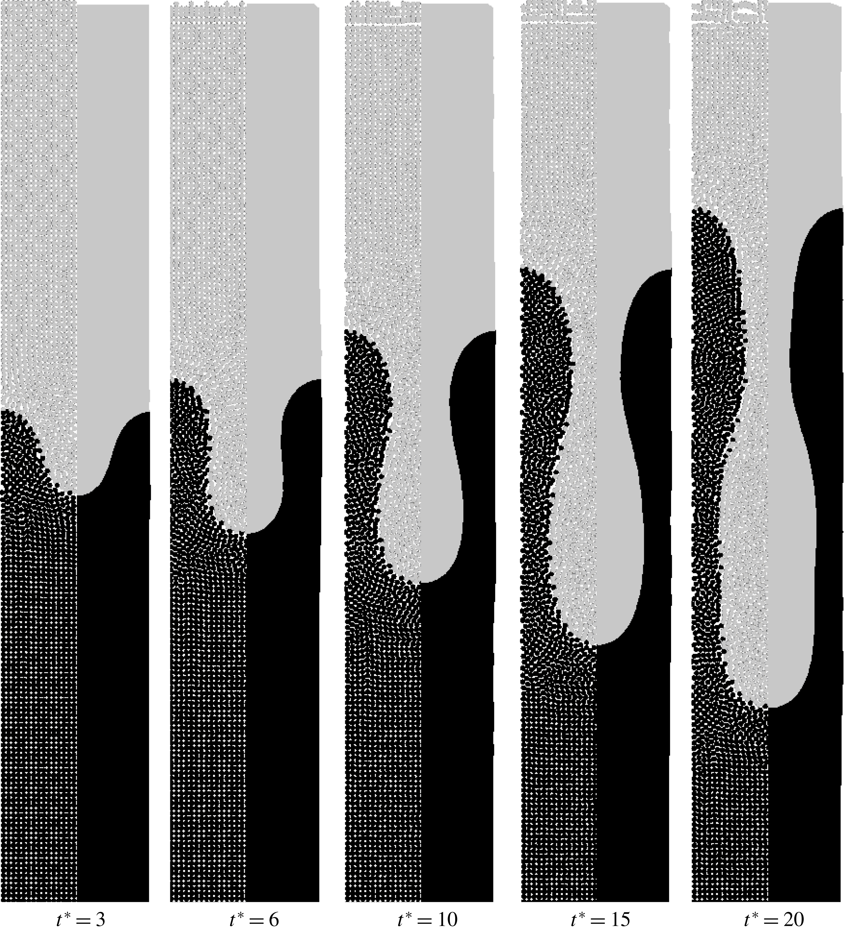
The time series demonstrates the evolution of a single finger. At first, a cylindrical finger grows. Then a contraction arises that leads to a bottleneck of the finger. At later times, the bottle-like finger elongates but the shape remains. There are two reasons for the bottleneck. The first reason is that the viscosity ratio
 $A$
is larger than the critical value of
 $A=0.2$
. It was found in Tryggvason & Aref (Reference Tryggvason and Aref1983) that bottlenecks are formed for higher viscosity ratios. Another reason may be the bounded domain. This phenomena is also seen in RTI (Rahmat, Tofighi & Yildiz Reference Rahmat, Tofighi and Yildiz2018).
Time evolution of immiscible viscous fingering of the maximum growth rate with wavelength of the perturbation
 $\unicode[STIX]{x1D706}=\unicode[STIX]{x1D706}_{m}$
. The density ratio is unity and the viscosity ratio is
 $A=1/3$
. On the left side the contour of the pressure is shown and on the right side the contour of the velocity is shown. The legends are found on the right side. The units of pressure
 $p$
and velocity
 $|v|$
are Pa and
 $\text{m}~\text{s}^{-1}$
.

Before analysing the velocity of displacement we have a closer look at the pressure and velocity fields in figure 12. On the left side of each plot in figure 12, the pressure contour is shown. On the right side of each plot, the magnitude of the velocity is shown. Each plot corresponds to the same sequential time as in figure 11.
The pressure field is almost identical in all time steps. It is linear along the flow direction, indicating Stokes’ flow. In contrast to that, the velocity increases from left to right. At early times the peak of the velocity is at the tip of the initial perturbation. At
 $t^{\ast }=10$
, when the finger starts to form a bottle-like shape, there are two different peaks in the velocity field. One peak is still located at the tip of the finger, but the second peak of similar magnitude is located at the contraction of the finger. This indicates that the contraction influences the dynamics of the growth of the finger as well. With increasing time, these two peaks remain but their distance increases along the finger.
Comparison of finger growth over time with power law for viscous fingering and flow in a channel for
 $\unicode[STIX]{x1D706}=\unicode[STIX]{x1D706}_{m}$
.

Next, we compare the growth of the finger with the power law of immiscible viscous fingering (3.11). We estimate the size of the finger by measuring the distance between the tip of the finger and its counterpart, e.g. the maximum distance between the interface of the phases in flow direction. We subtract the initial distance to account for the initial perturbation of the interface and calculate the dimensionless distance using (3.7) and (3.8).
In figure 13 the dimensionless distance is plotted over the dimensionless time. We compare the finger length taken from the simulation with different power laws. The first power law is
 $\unicode[STIX]{x1D717}^{\ast }\sim (t^{\ast })^{1.6}$
(3.11). The second power law in figure 13 is the linear dependence of the dimensionless finger length on the dimensionless time representing flow in a channel.
We identify two different regimes in figure 13. At small times (
 $t^{\ast }<7$
), we find a good agreement with the first power law (
 $\unicode[STIX]{x1D717}^{\ast }\sim (t^{\ast })^{1.6}$
) for immiscible viscous fingering. This indicates that the dynamics of growth of a cylindrical finger corresponds to immiscible viscous fingering. Up to this stage, the linear stability analysis is valid. For later times (
 $t^{\ast }>7$
), we find a growth of the finger in simulation
 $\unicode[STIX]{x1D717}^{\ast }\sim t^{\ast }$
. This indicates that the growth of the finger is dominated by the flow in the contraction and the finger is elongated by a laminar flow pattern. In the contraction, Stokes flow in a channel can be found because of the small gap
 $b$
. The dominating resistance in the momentum balance is the viscous resistance due to the gap and the dominating force is the pressure force. Therefore, assuming a constant velocity in the contraction, the evolution of the fluid linearly depends on the pressure force
 $$\begin{eqnarray}\text{d}x=\frac{b^{2}}{12\unicode[STIX]{x1D702}}\unicode[STIX]{x1D735}p\cdot \text{d}t.\end{eqnarray}$$
Therefore, the growth rate of the finger is dominated by a linear time relationship.
In experiments in § 2, we observed viscous fingering in the early stage of pore formation. Comparing figures 5 and 13, the same dynamics of growth of the finger is found, where in the early stages immiscible viscous fingering is present. It is later dominated by only viscous transport due to the contraction in the bottleneck of the finger.
4.2 Miscible viscous fingering
In this section, we study the dynamics of miscible viscous fingering to identify possible effects on pore formation. We consider the (binary) component and momentum balance but neglect surface tension as well as the gradient term in the chemical potential because their effects are very small. Therefore, we exchange the chemical potential in the driving force by
 $\unicode[STIX]{x1D714}$
. Then, the component balance simplifies to a Fickian diffusion equation. In addition, we assume that the viscosity depends on
 $\unicode[STIX]{x1D714}$
. The simulation parameters are summarized in table 4.
The wavelength of the initial perturbation is altered by varying the mobility coefficient. The set-up is the same as the one for immiscible viscous fingering including the initial perturbation shown in (4.1). The value of the constant
 $\unicode[STIX]{x1D6FD}$
in (3.14) is 2 assuming that the maximum concentration in the system is
 $\unicode[STIX]{x1D714}_{max}=0.5$
. The initial concentrations are
 $\unicode[STIX]{x1D714}_{1}=0$
and
 $\unicode[STIX]{x1D714}_{2}=0.5$
. We investigate the limit of stability, compare it to the theoretical value and analyse the dynamics of displacement.
4.2.1 Limit of stability of displacement
We keep all simulation parameters except the mobility coefficient constant. Therefore, the wavelength of the initial perturbation increases linearly with the mobility coefficient.
The distribution of mass fractions for five different mobility coefficients are shown in figure 14 at time
 $t^{\ast }=8$
. On the left side particle distributions are shown and on the right side smooth contour plots are shown. The grey scale indicates the concentration in the range of
 $\unicode[STIX]{x1D714}\in [0,0.5]$
. Instead of the critical wavelength, we consider the critical mobility coefficient
 $M_{c}$
.
First, we consider the case
 $M=M_{c}$
(figure 14
e). Similar to immiscible viscous fingering, the displacement is stable for the critical value
 $M=M_{c}$
. When we decrease the mobility coefficient to
 $M=85\,\%M_{c}$
we still do not find propagation of a finger. We quantitatively confirm this observation by analysing
 $\unicode[STIX]{x1D717}^{\ast }$
over time and find exactly
 $\unicode[STIX]{x1D717}^{\ast }\sim \sqrt{t^{\ast }}$
. This indicates that dispersion is the dominant mechanism.
Stability of miscible viscous fingering with different wavelengths of the perturbation at
 $t^{\ast }=8$
. The limit of stability is between
 $M=21\,\%M_{c}$
and
 $M=47\,\%M_{c}$
. The density ratio is unity and the viscosity ratio is
 $A=1/3$
. On the left side the particle distribution is shown and on the right side the contour plot of the two phases is shown. For
 $M=0.01\,\%M_{c}$
the time is
 $t^{\ast }=1.6$
.

Then, we further decrease the mobility coefficient to
 $M=47\,\%M_{c}$
. This is the case of the maximum growth rate according to the theory. We see that a finger evolves slowly but as we will see later only by dispersion. Therefore, the limit of stability is around
 $M=47\,\%M_{c}$
. When we further decrease the mobility coefficient, we observe fingering (figure 14
b). In the limit of a very low mobility coefficient, where the wavelength of stability is below the numerical resolution, we observe stochastic-like mixing of the phases. This case is added for completeness, but clearly, we do not observe fingers because any perturbation of the interface leads to mixing of the fluids. It is noted that, as for immiscible fingering, the perturbation does not disturb the pressure field at the interface.
Time evolution of miscible viscous fingering with the maximum growth rate with wavelength of the perturbation
 $\unicode[STIX]{x1D706}=\unicode[STIX]{x1D706}_{m}$
. The density ratio is unity and the viscosity ratio is
 $A=1/3$
. On the left side the particle distribution is shown and on the right side the contour plot of the two phases is shown.

We found that the limit of stability is around
 $M=47\,\%M_{c}$
. This is clearly lower than predicted by the theory. A reason may be that the critical wavelength was derived by assuming a sharp interface but enable dispersion over the interface. In the simulations we find a very diffuse interface between the fluids. This is in contrast with the assumptions used in theoretical studies. A diffuse interface increases the size of the initial perturbation due to dispersion. Therefore, the wavelength is changed to a larger value. To compensate this, the wavelength of the initial perturbation needs to be smaller than the critical value from theory.
4.2.2 Analysis of the dynamics of displacement
Next, we analyse the dynamics of displacement for miscible viscous fingering. We consider the case with maximum growth rate
 $\unicode[STIX]{x1D706}=\unicode[STIX]{x1D706}_{m}$
. The particle distribution and the contours of the mass fraction at
 $t^{\ast }=1.5$
, 3, 4.5, 6 and 8 are shown in figure 15. The grey scale is divided into 10 steps so that iso-lines are visible. We observe that the finger evolves and the mixing area between the fluids increases with time. We also observe that the shape of the initial perturbation remains similar, as may be seen from the iso-lines. This indicates that dispersion in the direction of the flow dominates and viscous fingering dynamics may be small. We demonstrate this in figure 16(a). The size of the mixing area
 $\unicode[STIX]{x1D717}^{\ast }$
versus time
 $t^{\ast }$
for
 $M=10\,\%M_{c}$
,
 $M=21\,\%M_{c}$
and
 $M=47\,\%M_{c}$
is shown in figure 16(a). As a reference we plot (3.18) too. We see that
 $M=47\,\%M_{c}$
follows the scaling law for dispersion
 $\unicode[STIX]{x1D717}\sim \sqrt{t^{\ast }}$
(3.18). Only at larger times the growth of the mixing area is larger and slowly changes to miscible fingering dynamics. The transition to fingering dynamics is faster for lower mobility coefficients as shown in figure 16(a) for the cases
 $M=21\,\%M_{c}$
and
 $M=10\,\%M_{c}$
.
(a) Comparison of finger growth over time with the theory of Pramanik & Mishra (Reference Pramanik and Mishra2015) for different wavelengths. (b) Comparison of one wavelength (
 $M=10\,\%M_{c}$
) with the power law for diffusive transport
 ${\sim}\sqrt{t^{\ast }}$
and power law similar to immiscible viscous fingering
 ${\sim}(t^{\ast })^{0.8}$
.

There remains the question about the scaling law for miscible viscous fingering when the dynamics is dominated by the instability instead of dispersion. The dynamics of fingering instability may be similar in miscible and immiscible systems. For immiscible systems we found that
 $\unicode[STIX]{x1D717}^{\ast }\sim (t^{\ast })^{1.6}$
and for later times, when only flow through a channel is dominant,
 $\unicode[STIX]{x1D717}^{\ast }\sim t^{\ast }$
. For miscible systems we may expect a similar behaviour with a transition from the dynamics of dispersion, viscous fingering and flow through a channel.
We demonstrate the scaling law for
 $M=10\,\%M_{c}$
in figure 16(b). We found that
 $\unicode[STIX]{x1D717}^{\ast }\sim \sqrt{t^{\ast }}$
at the early times when dispersion is dominant. For later times, we observe a transition to
 $\unicode[STIX]{x1D717}^{\ast }\sim \sqrt{(t^{\ast })^{1.6}}$
. We have not observed a third transition in the simulations. The reason is that the finger never formed a bottleneck.
When comparing figure 16 to the experiments in figure 5 we find disagreements between the finger pores in the experiments and the dynamics of miscible viscous fingering. One possible reason is the small driving force in the experiments (capillary forces between the glass plates) and, therefore, the diffusion dominates the system. As a consequence, the growth of finger pores after the initial contact of the polymer solution and the coagulation bath is not affected by miscible viscous fingering.
In experiments it was observed that finger pores or macrovoids originate inside of the polymer solution (Yu et al. Reference Yu, Yang and Xiang2014). The formation of finger pores inside of the polymer solution due to miscible viscous fingering is very unlikely because of the absence of the driving force. Hence, we conclude that miscible viscous fingering is not present in pore formation.
4.3 The more general case: immiscible viscous fingering with diffusive mass transport
Until now, we assumed that the interface between two stable, immiscible fluids is sharp and, therefore, calculated the surface tension using a sharp colour function. In this section, we investigate the formation of a viscous finger in a phase separating and a more viscous fluid mixture where the surface tension and diffusive mass transfer across the interface are present. Consequently, we calculate the normal in (3.35) based on the mass fraction, similar to the smoothed colour function by Shadloo et al. (Reference Shadloo, Zainali and Yildiz2012a ).
The numerical set-up is the same as the previous ones. The surface tension is
 $\unicode[STIX]{x1D70E}=34.68~\text{mN}~\text{m}^{-1}$
. Additional parameters are summarized in table 4. Note that we consider a binary mixture where phase 1 corresponds to a mass fraction
 $\unicode[STIX]{x1D714}<0.5$
and phase 2 corresponds to a mass fraction
 $\unicode[STIX]{x1D714}\geqslant 0.5$
. We consider a linear relationship of the viscosity on the mass fraction. The viscosity ratio varies between
 $A=1/4$
and
 $A=1/2$
over time during phase separation of the more viscous mixture. The mobility coefficient in component balance is
 $M=9.7829\times 10^{-7}~\text{m}~\text{s}^{-1}$
to keep the interface as thin as possible without losing smoothness. The chemical potential is calculated using (3.33) with an interaction parameter
 $\unicode[STIX]{x1D712}=3$
. We consider the case for maximum growth rate with
 $\unicode[STIX]{x1D706}=\unicode[STIX]{x1D706}_{m}$
for immiscible viscous fingering.
The time series of the contour compared to the results for the immiscible fingering (figure 11) are shown in figure 17. On the left side the previous results and on the right side the results with a diffuse interface are shown. The colour indicates the concentration
 $\unicode[STIX]{x1D714}\in [0.1,0.5]$
in 10 steps. Higher and lower concentrations are clipped to enable direct comparison.
Time evolution of immiscible viscous fingering without (left) and with (right) the Cahn–Hilliard equation with the maximum growth rate and
 $\unicode[STIX]{x1D706}=\unicode[STIX]{x1D706}_{m}$
. The density ratio is unity and the viscosity ratio is
 $A=1/3$
. The contour of the two phases is shown with the grey scale fitted to
 $\unicode[STIX]{x1D714}\in [0.1,0.5]$
in 10 steps. Lower and larger concentrations are clipped.

We see that the interface between the fluids is diffuse but the growth of the finger tip is similar. Therefore, we conclude that the dynamics of immiscible fingering is almost unchanged by the diffuse interface. At later times, we see small deviation at the bottleneck of the finger. The length of the bottleneck is shorter in the diffuse case. Reasons for this are the dispersion effect in the radial direction and an increment of the viscosity in the dark phase, because the system tends to phase separate. Therefore, the mass fraction increases near the interface in the dark phase. Similar effects are observed in the experiments in § 2 for different viscosity ratios.
4.3.1 Influence of different mobility coefficient on the shape of fingers
Next, we investigate the influence of different mobility coefficients on the shape of fingers by altering the mobility coefficient between
 $M=10^{-7}~\text{m}^{2}~\text{s}^{-1}$
and
 $M=10^{-5}~\text{m}^{2}~\text{s}^{-1}$
.
The shape of viscous fingers for three mobility coefficients are shown in figure 18. All shapes are shown at the same time step
 $t=150~\text{s}$
. The grey scale indicates the composition where a dark area represents a polymer-rich region. With increasing mobility coefficient, we see that the polymer-rich phase is darker, indicating that phase separation is present. The colour of the polymer-lean phase is almost identical. At the tips of the fingers we observe very different behaviour. For small mobility coefficients, we see that the influence of diffusion is very small. The interface between the phases is scattered and we do not have a smooth diffuse interface. Numerically, such a system is not appropriately resolved because the diffuse interface evolves too slowly compared to the motion of the fluid. Figure 18(c) is shown here for completeness.
Shape of viscous finger at time
 $t=150~\text{s}$
. Influence of different magnitudes of mobility coefficient during viscous fingering. From (a) to (c) we decreased the mobility coefficient by a factor of 10. The grey scale indicates the composition where black represents pure polymer in the polymer-rich phase.

For a medium mobility coefficient (figure 18 b), the interface between the phases is smooth and a single finger is observed. We identify an increase in the polymer content at the interface aligned parallel to the interface. This is because phase 2 starts to phase separate forming a dense layer. In this case, the displacement is of the same magnitude as the dispersion.
For higher mobility coefficients, we find faster smoothing of the mass fraction than convective motion of the finger. We observe phase separation in the finger tip front. We also observe a stable alternating lamella followed by a bubble in front of the tip. We do not observe finger pores. The pore structure is very similar to the Liesegang rings in § 2. To highlight this similarity, we investigate the pore structure in more detail.
In figure 19, a time series of the simulation using
 $M=10^{-5}\text{m}^{2}~\text{s}^{-1}$
is shown, where time increases from top to bottom. We observe a viscous finger and evolving Liesegang rings. The alternating structures indicate a diffusion front in front of the finger. The diffusion front evolves faster than the viscous finger. In addition, the viscous finger evolves not only by convective transport but also by coalescence of the finger tip with a lamella.
Time series of the shape of a viscous finger with
 $M=10^{-5}\text{m}^{2}~\text{s}^{-1}$
. Increasing time from (a) to (e). The grey scale indicates the composition where black represents pure polymer in the polymer-rich phase.

Evolution of diffusion front over time for the case
 $M=10^{-5}~\text{m}^{2}~\text{s}^{-1}$
. The power law is a fit of the simulation data.

Quantitatively, the dynamics of the viscous finger is analysed by estimating the distance between the initial position of the finger tip and the position of the leading lamella over time (see figure 20). The simulation data are shown as symbols and the solid line represents a power law fit. The simulation data are not smooth because we identify the diffusion front using a threshold for the composition
 $\unicode[STIX]{x1D714}>0.5$
on the alternating lamella. It is noted that the jumps in the lower lines are caused by coalescence of the structures. The slope of the fitted power law is approximately 0.7. For pure diffusion we would expect a slope of 0.5 as shown for the experiments in figure 5. Nevertheless, it is much smaller than the slope for viscous fingering.
In § 2, we observe the formation of dense layers by pure diffusion. In the simulations, when we consider both viscous fingering and phase separation of a polymer solution, we observe that a dense layer is formed, behind which no viscous fingers originate. This is in contradiction with the experimental results of Yu et al. (Reference Yu, Yang and Xiang2014) where it was found that finger pores originate behind dense layers or sponge pore structures. The formation of finger pores cannot be explained with the mechanism of viscous fingering because of, firstly, the absence of the driving force for fingering and, secondly, because fingers should have been originated previously due a comparable viscosity ratio at the precipitation front.
In previous studies, it was often not considered that the experiments were performed in the Hele-Shaw cell. It is known that Hele-Shaw cells promote viscous fingering. Since the mechanism of viscous fingering does not explain the formation of every pore structure, it seems likely that observation of the viscous fingering dynamics in pore formation is an artefact of the experimental set-up and not the mechanism of pore formation. Therefore, we conclude that there must be another mechanism that explains the formation of sponge, finger and dense layer structures.
5 Conclusion
In the first part of the current work we reviewed experimental observations and proposed theories on the formation of pores during the preparation process of polymer membranes. The theories are diverse because they rely, on the one hand, on diffusive transport and, on the other hand, on convective transport of the solvent and non-solvent. Therefore, we reproduced some experiments, similar to the experiments published by Strathmann et al. (Reference Strathmann, Kock and Amar1975) with higher time resolution, to investigate the dynamics of finger and sponge pore formation. We found that by adding a pore builder (PVP) to the polymer solution a transition from finger pores to sponge pores is possible. By analysing the motion of the precipitation front, we found evidence for immiscible viscous fingering at the early stage of finger pore formation. Interestingly, viscous fingering is only present at the first moments of contact between the polymer solution and the coagulation bath, even though finger pores evolve. At later times other effects may dominate, e.g. convective flow in a channel. This finding is confirmed by the numerical results for the immiscible viscous fingering. At the early stage of finger formation, the growth dynamics of immiscible viscous fingering agrees well between experiment and simulation results. At later times, a bottleneck is formed and viscous transport driven by capillary forces between the glass plates through the bottleneck dominates further growing of the finger. This was observed both in simulations and experiments. Therefore, we conclude that immiscible viscous fingering is present in the early stage of pore formation and viscous transport propagates the growth of finger pores.
Based on these findings, we focused on viscous fingering and diffusive transport in the remainder of this work to numerically investigate the early evolution of viscous fingers. We investigated immiscible and miscible viscous fingering separately. We demonstrated that our model predicts the immiscible viscous fingering within a reasonable accuracy compared to previous studies on Rayleigh–Taylor instability (RTI) where we found that within a deviation of 15–20 % the model matches the stability criterion. Usually, viscosity is neglected in the analytical approach that may be another source of error. An analysis of the growth of a single finger shows that the finger grows with the super-linear power law until the time that the contraction of the finger is formed for immiscible fluids. The same behaviour was found in the previous experiments. In contrast, investigations of miscible viscous fingering indicate that the time evolution of finger growth scales with
 $\unicode[STIX]{x1D717}^{\ast }\sim \sqrt{(t^{\ast })^{1.6}}$
.
We also demonstrated that a diffuse interface between the fluids leads to similar results than a sharp interface. For a diffuse interface we need to specify a mobility coefficient in the component balance. We varied the mobility coefficient and demonstrated that for large mobility coefficients Liesegang rings are visible. Dense layer structures, similar to Liesegang rings, were previously observed in the experiments. The dynamics of evolution of rings formation is purely diffusive. This was confirmed by the simulations. Dense layers are formed when phase separation dynamics dominates over the propagation of viscous fingering. Fingers grow mainly by coalescence of lamella with the finger tip. We conclude that further analysis on the formation of dense layers is necessary to clarify its relevance for pore formation.
In the present form, the numerical results do not help to explain the formation of sponge versus finger pores at different polymer concentrations. The reason is not the numerical model (which in principle is complete), but the numerical set-up because a precipitation front should move towards the polymer solution. Here, we implicitly considered an infinitely large velocity of the precipitation front. Therefore, the formation of finger pores due to phase separation is not possible and fingers can only originate by viscous fingering. In future work, enslaved pore formation behind a moving precipitation front should be investigated in the context of porous polymer membranes. Recently, Foard & Wagner (Reference Foard and Wagner2012) presented the first results indicating the significance of the velocity of a moving precipitation front on the formation of porous structures.
Acknowledgements
M.H.-H. and U.N. gratefully acknowledge financial support from the German Research Foundation (DFG) within the Collaborative Research Centre 716. M.H.-H. acknowledges financial support from the Max Buchner Research Foundation through funding ID MBFSt 3675. M.S.S. acknowledges funding provided by DAAD program ‘Research Stays for University Academics and Scientists, 2017’ through funding ID: 57314019 during his visit from Stuttgart University. The access to the French CRIANN (Centre Régional Informatique et d’Applications Numériques de Normandie) resources, under allocation 2017002, is also acknowledged. This work was granted access to HPC resources of IDRIS under the allocation 2017-100752 made by GENCI (A0022A10103).
Appendix A
Here we present the detailed results of measurements of viscosity. The viscosity is determined using the rotational rheometer RheoStress 600 from HAAKE with a titanium cone and a diameter of 35 mm with an angle of
 $1^{\circ }$
at constant temperature
 $T=293.15~\text{K}$
. The shear stress symb:taustress is measured at constant rate symb:gammastress for different rates. The dynamic viscosity
 $\unicode[STIX]{x1D702}$
is calculated in the software RheoWin from HAAKE. Each measurement is repeated three times. The plots show the arithmetic average of shear stress over shear rate and dynamic viscosity over shear rate for each mixture indicated in table 2. The error bars indicate the maximum and minimum values.
Shear stress and viscosity for different shear rates: 12 % PSf – 88 % NMP.

Shear stress and viscosity for different shear rates: 15 % PSf – 85 % NMP.

Shear stress and viscosity for different shear rates: 20 % PSf – 80 % NMP.

Shear stress and viscosity for different shear rates: 25 % PSf – 75 % NMP.

Shear stress and viscosity for different shear rates: 25 % PSf – 69 % NMP – 6 % PVP.

Appendix B
In this appendix the algorithm of the incompressible SPH (ISPH) approach is presented in detail. The particles are initially located in the computational domain in the regular Cartesian order where the values of composition
 $\unicode[STIX]{x1D714}(t=0)$
, velocity
 $\boldsymbol{u}(t=0)$
and the mass
 $m$
of each particle are assigned. The volume of each particle is specified by the definition of the smoothing length of the kernel function.
Algorithm of ISPH approach.

Then, we perform the time marching for the time period
 $t<t_{max}$
(see figure 26). During this loop, we first build up the neighbour list using a cell list, calculate the density
 $\unicode[STIX]{x1D70C}$
(3.31), correct kernels of each particle (3.42) and (3.46) and update the periodic boundary conditions.
In the next step, the calculation of the acceleration of particle
 $a$
in the predictor step,
 $$\begin{eqnarray}\boldsymbol{a}_{a,\ast }=\mathop{\sum }_{b}\frac{m_{b}}{\unicode[STIX]{x1D70C}_{a}\unicode[STIX]{x1D70C}_{b}}(\unicode[STIX]{x1D702}_{a}+\unicode[STIX]{x1D702}_{b})\frac{\boldsymbol{r}_{ab}}{r_{ab}^{2}}\unicode[STIX]{x1D735}_{a}W_{ab}\boldsymbol{\cdot }(\boldsymbol{u}_{a}-\boldsymbol{u}_{b})+\frac{|\boldsymbol{n}_{a}|}{\unicode[STIX]{x1D70C}_{a}}(\unicode[STIX]{x1D70E}_{a}\unicode[STIX]{x1D705}_{a}\hat{\boldsymbol{n}}_{a}),\end{eqnarray}$$
splits into two parts because an update of the boundary conditions is necessary in between. First we calculate the viscous term and the normal in the momentum balance (3.35) and (3.36) as well as the gradient term of the chemical potential (3.34) in the component balance. Then, the periodic boundaries are updated and a second set of corrected kernels are calculated considering only particles with a normal larger than
 $0.01h$
.
Then the interface curvature (3.37), the total surface tension in the momentum balance (3.35) and the new composition
 $\unicode[STIX]{x1D714}(t+1)$
are calculated. The composition is integrated using an explicit Euler step
 $$\begin{eqnarray}\unicode[STIX]{x1D714}(t+1)_{a}=\unicode[STIX]{x1D714}(t)_{a}+\frac{\text{d}\unicode[STIX]{x1D714}_{a}}{\text{d}t}\unicode[STIX]{x0394}t.\end{eqnarray}$$
Afterwards, the intermediate velocity
 $\boldsymbol{u}_{a,\ast }$
is calculated using an explicit Euler step
 $$\begin{eqnarray}\boldsymbol{u}_{a,\ast }=\boldsymbol{u}(t)_{a}+\boldsymbol{a}_{a,\ast }\unicode[STIX]{x0394}t,\end{eqnarray}$$
with the time step
 $\unicode[STIX]{x0394}t$
and the velocity of the previous time step
 $\boldsymbol{u}(t)_{a}$
.
After updating the periodic boundaries, PPE (3.38) is built up by first calculating the divergence of the intermediate velocity
 $$\begin{eqnarray}\frac{\unicode[STIX]{x1D735}\boldsymbol{\cdot }\boldsymbol{u}_{a,\ast }}{\unicode[STIX]{x0394}t}=\frac{1}{\unicode[STIX]{x0394}t}\mathop{\sum }_{b}\frac{m_{b}}{\unicode[STIX]{x1D70C}_{b}}(\boldsymbol{u}_{b,\ast }-\boldsymbol{u}_{a,\ast })\unicode[STIX]{x1D735}_{a}W_{ab},\end{eqnarray}$$
and then setting up the linear equation system (LES)
 $$\begin{eqnarray}\unicode[STIX]{x1D735}\boldsymbol{\cdot }\left(\frac{\unicode[STIX]{x1D735}p}{\unicode[STIX]{x1D70C}_{\ast }}\right)=\frac{\unicode[STIX]{x1D735}\boldsymbol{\cdot }\boldsymbol{u}_{\ast }}{\unicode[STIX]{x0394}t},\end{eqnarray}$$
with
 $$\begin{eqnarray}\unicode[STIX]{x1D735}\boldsymbol{\cdot }\left(\frac{\unicode[STIX]{x1D735}p}{\unicode[STIX]{x1D70C}_{a}}\right)_{a}=\mathop{\sum }_{b}2\frac{m_{b}}{\unicode[STIX]{x1D70C}_{b}\unicode[STIX]{x1D70C}_{a}}\cdot (p_{a}-p_{b})\frac{\boldsymbol{r}_{ab}}{r_{ab}^{2}}\unicode[STIX]{x1D735}_{a}W_{ab}.\end{eqnarray}$$
The LES is solved using a stabilized version of the biCGStab method from the PETSc library with a boomerAMG preconditioner from the HYPRE library.
After updating the periodic boundary conditions, the acceleration in the corrector step
 $$\begin{eqnarray}\boldsymbol{a}_{a,\ast \ast }=-\mathop{\sum }_{b}\frac{m_{b}}{\unicode[STIX]{x1D70C}_{a}\cdot \unicode[STIX]{x1D70C}_{b}}(p_{b}+p_{a})\unicode[STIX]{x1D735}_{a}W_{ab},\end{eqnarray}$$
is calculated. Before integrating the new velocity and position of the particles, we check for the CFL criterion. If the time step is accepted, we integrate the velocity
 $$\begin{eqnarray}\boldsymbol{u}(t+1)_{a}=\boldsymbol{u}_{a,\ast }+\boldsymbol{a}_{a,\ast \ast }\unicode[STIX]{x0394}t,\end{eqnarray}$$
and position
 $$\begin{eqnarray}\boldsymbol{x}(t+1)_{a}=\boldsymbol{x}(t)_{a}+\frac{\boldsymbol{u}(t)_{a}+\boldsymbol{u}(t+1)_{a}}{2}\unicode[STIX]{x0394}t.\end{eqnarray}$$
If the time step is rejected we withdraw all calculations and repeat the time loop using the time step due to the CFL criterion.
The last step in the time loop is to apply the shifting procedure. This requires us to update the density and periodic boundary conditions to correctly apply the projection of the particle-related properties to the new position after shifting.



