Antenna design

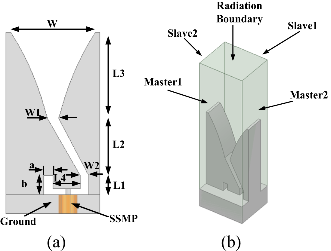
The all-metal Vivaldi antenna is composed of a radiating part (the flare notch) and a feeding part, as illustrated in Fig. 1(a). Similar to the PCB-based Vivaldi antennas, the radiating part employs an exponentially tapered aperture to achieve effective impedance matching. The feeding part is composed of a slot-line and a cavity, designed to achieve both impedance matching and energy transmission. Compared to microstrip-to-slot-line transition of traditional PCB-based designs [Reference Shin and Schaubert22] and the Marchand balun [Reference Marchand23], the feeding part transfers energy directly from the coaxial connector into the slot-line. Furthermore, unlike previous element designs [Reference Ma, Chai, Xiao and Ding21, Reference Kindt and Pickles24–Reference Ma, Guan, Li, Fan and Chen27], the proposed antenna removes the metal portion between the slot-line and the ground, integrating the feeding part with the ground. This integration thus liberates connector selection from the constraint of antenna thickness. The element is roughly 2/3λ in width, 1/3λ in thickness, and 1λ in height, where λ represents the wavelength at the high-frequency end of the band. The actual element lattice spacing is 4.2 mm × 5.0 mm, which is primarily determined by the requirement to suppress grating lobes within the operational scanning range.

Figure 1.

Metal Vivaldi element. (a) Side view of the element and (b) element simulation model.

Figure 1 Long description

The image A showing a dimensioned geometry drawing of a tapered slot element above a base labeled Ground, with a central tapered opening that widens toward the top and narrows toward the bottom. A double headed horizontal dimension arrow spans the top opening and is labeled W. Two inward pointing arrows near the mid height point to the two inner edges of the taper, with the left arrow labeled W1 and the right arrow labeled W2. Along the right side, three stacked vertical double headed dimension arrows run from near the top toward the base and are labeled L3, L2 and L1. Near the lower left of the tapered opening, two short horizontal double headed dimension arrows are labeled a and L4 and a vertical double headed dimension arrow beside them is labeled b. At the bottom center, a rectangular feed feature extends downward below the Ground region and is labeled SSMP by an arrow. No numeric values or units are printed for W, W1, W2, L1, L2, L3, L4, a, or b. The image B showing a three dimensional rectangular enclosure around the same tapered element, with a downward arrow pointing to the top face labeled Radiation Boundary. Four arrows point to faces of the enclosure labeled Slave2, Slave1, Master1 and Master2. Inside the enclosure, the tapered element rises from a base block and the enclosure surfaces labeled Master1, Master2, Slave1 and Slave2 are shown as paired boundary faces while the Radiation Boundary label is attached to the top face.

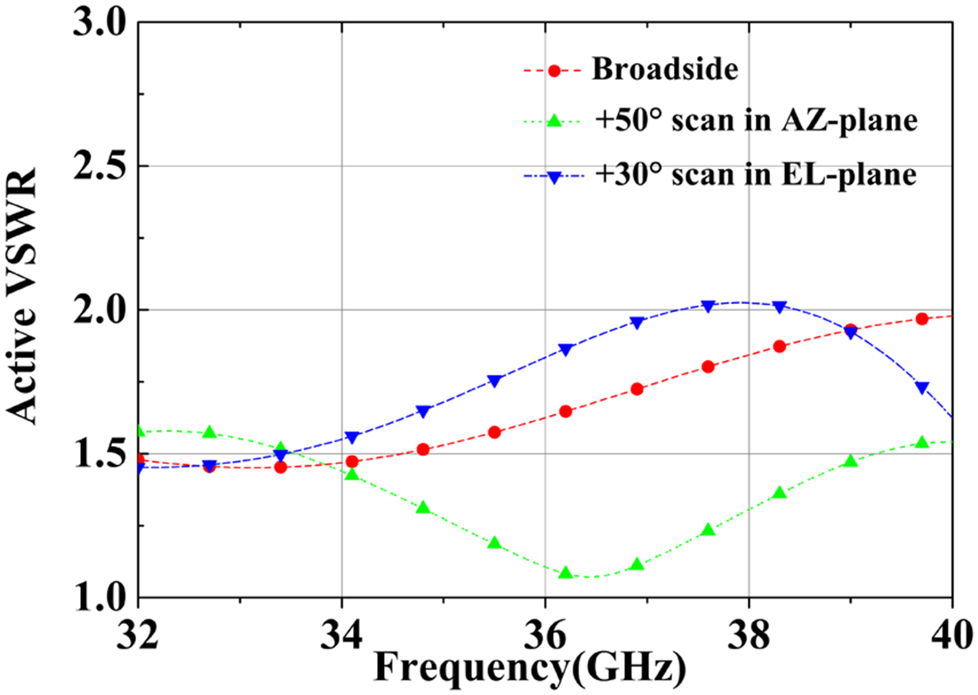
The element was simulated and optimized with ANSYS using periodic boundaries, as shown in Fig. 1(b). Its optimized dimensions are summarized in Table 1. As shown in Fig. 2, the simulated VSWR remains below 2 across the entire band at broadside. Under scanning conditions, the VSWR is below 1.6 at +50° in the AZ-plane and below 2 at +30° in the EL-plane. These results confirm the element’s good impedance matching across the operational bandwidth and within the specified scan range.

Table 1.

Model dimensions (mm)

Table 1 Long description

The table lists a single set of model dimensions measured in millimeters across width, multiple length segments, and two additional parameters labeled a and b. The width W is 4, while the related widths W1 and W2 are 1 and 0.6, making W2 the smallest width value. The length values are L1 1.5, L2 2.5, L3 3.5, and L4 2, with L3 being the largest length and L1 the smallest. Among the lengths, L2 is larger than L4, and L4 is larger than L1. Parameter a is 1 and parameter b is 1.5, so b is larger than a. Only one row of measurements is provided, so no variation across models or conditions can be inferred.

Figure 2.

Simulated VSWR of element.

Array simulation

The array comprises 28 linear sub-arrays, each containing 6 elements. These sub-arrays were monolithically fabricated from aluminum using high-precision wire electrical discharge machining, achieving a dimensional tolerance of ±0.02 mm (Fig. 3).

Figure 3.

Six-element linear sub-array.

Following the initial element design via unit-cell simulation under periodic boundary conditions, a full 28 × 6 array model was constructed for more accurate full-wave analysis. The array is configured with 28 elements in the AZ-plane and 6 elements in the EL-plane. To accurately model the physical assembly, a 0.2 mm gap was introduced between adjacent linear sub-arrays in the simulation. The complete model is shown in Fig. 4.

Figure 4.

Top view of array simulation model.

The polarizer comprises two layers of metallic strips, as illustrated in Fig. 5. The strips in the first layer are perpendicular to the incident electric field, while those in the second layer are oriented at a 45° angle. Both layers have identical strip widths and inter-strip gaps of 1 mm. The dielectric between them is a Rogers 5880 substrate with a thickness of 1.5 mm.

Figure 5.

Geometry of the polarizer.

The combined array and polarizer model is shown in Fig. 6. To accommodate the beam scanning range and the required placement height of the polarizer, the polarizer’s aperture was enlarged relative to the array aperture.

Figure 6.

Simulation array model with polarization converter.

The active VSWR of the six elements in the 14th azimuth column across the scanning range is shown in Fig. 7. The simulated values remain below 2.8 within the band, confirming acceptable impedance matching. Moreover, their variation trend agrees well with the unit-cell simulation results obtained under periodic boundary conditions (Fig. 2).

Figure 7.

Simulated active VSWR of center six-element sub-array for (a) broadside radiation, (b) +30° scan in EL-plane, and (c) +50° scan in AZ-plane.

Figure 7 Long description

The graphs display active VSWR against frequency in GHz for six elements. The horizontal axis is labeled Frequency(GHz) ranging from 32 to 40 and the vertical axis is labeled Active VSWR ranging from 1.0 to 3.0. The legend identifies Element 1 through Element 6. In graph (a), broadside radiation, Element 1 shows a peak around 38 GHz, while Element 6 remains relatively stable. In graph (b), 30-degree EL-plane, Element 2 peaks near 36 GHz, with Element 5 showing a dip around 34 GHz. In graph (c), 50-degree AZ-plane, Element 3 has a noticeable rise at 37 GHz and Element 4 shows a decline after 38 GHz. Each line is distinguished by different symbols for clarity. The graphs illustrate variations in active VSWR across different scanning scenarios, highlighting impedance matching performance.

Figure 8 shows the simulated, normalized H- and V-pol radiation patterns versus scan angle. Across the entire band and scan range, the amplitude difference between the two components remains below 2.6 dB, demonstrating excellent purity of the 45° slant polarization.

Figure 8.

Simulated normalized patterns at broadside and scan angles of ±25° and ±50° in the AZ-plane and ±30° in the EL-plane. (a) 32 GHz in AZ-plane (left) and EL-plane (right), (b) 36 GHz in AZ-plane (left) and EL-plane (right), (c) 40 GHz in AZ-plane (left) and EL-plane (right).

Figure 8 Long description

The image consists of six line graphs displaying simulated normalized patterns at broadside and scan angles in the AZ-plane and EL-plane. Each graph compares H-pol and V-pol patterns. The x-axis is labeled ‘Angle (degrees)’ ranging from -90 to 90 degrees. The y-axis is labeled ‘Normalized Amplitude (dB)’. (a) Shows patterns at 32 GHz in the AZ-plane (left) and EL-plane (right). (b) Shows patterns at 36 GHz in the AZ-plane (left) and EL-plane (right). (c) Shows patterns at 40 GHz in the AZ-plane (left) and EL-plane (right). Each graph features multiple lobes and deep nulls, with H-pol and V-pol curves distinguished by solid and dashed lines. Key features include peak directions and null angles, demonstrating the amplitude difference between the two polarizations remains below 2.6 decibels across the band and scan range.

Results and discussion

A 28 × 6 array prototype, measuring 117.6 mm × 33 mm × 7.5 mm, was fabricated. Figure 9 shows photographs of the array; the polarizer is omitted to reveal the layout of the sub-arrays. The active VSWR was measured using an Agilent N5244A vector network analyzer, while the radiation patterns and gain were measured in a microwave anechoic chamber. For the pattern measurements, each linear sub-array was connected to a six-channel T/R module to enable independent control of the amplitude and phase of each element.

Figure 9.

28 × 6 element array constructed from modular sub-arrays.

The active VSWR was measured for each element using an S-parameter synthesis procedure [Reference Marchand23]. Results for three representative elements are presented in Fig. 10: edge element 1 (Row 1, Column 1), edge element 4 (Row 4, Column 1), and center element 82 (Row 4, Column 14), whose locations are indicated in Fig. 9. As shown in Fig. 10, all measured values remain below 2.6. As expected, the edge elements exhibit higher active VSWR than the center element due to array truncation effects. Furthermore, the active VSWR of the center elements is comparable to the results presented in Fig. 2.

Figure 10.

Measured active VSWR for elements (1), (4), and (82) in the 28 × 6 element array.

Figure 10 Long description

A) element (1). The y-axis is labeled Active VSWR, ranging from 1.0 to 3.0 with ticks at 1.0, 1.5, 2.0, 2.5, 3.0. The x-axis is labeled Frequency(GHz), ranging from 32 to 40 with ticks at 32, 34, 36, 38, 40. Legend entries are Broadside, plus 30 degree scan in EL-plane, plus 50 degree scan in AZ-plane. Broadside values: 32 about 1.65, 33 about 1.50, 34 about 1.55, 35 about 1.55, 36 about 1.45, 37 about 1.30, 38 about 1.10, 39 about 1.50, 40 about 2.50. Plus 30 degree scan in EL-plane values: 32 about 1.45, 33 about 1.40, 34 about 1.50, 35 about 1.60, 36 about 1.60, 37 about 1.60, 38 about 1.90, 39 about 1.70, 40 about 1.45. Plus 50 degree scan in AZ-plane values: 32 about 1.25, 33 about 1.30, 34 about 1.45, 35 about 1.70, 36 about 1.90, 37 about 2.20, 38 about 2.25, 39 about 1.85, 40 about 1.20. B) element (4). The y-axis is labeled Active VSWR, ranging from 1.0 to 3.0 with ticks at 1.0, 1.5, 2.0, 2.5, 3.0. The x-axis is labeled Frequency(GHz), ranging from 32 to 40 with ticks at 32, 34, 36, 38, 40. Legend entries are Broadside, plus 30 degree scan in EL-plane, plus 50 degree scan in AZ-plane. Broadside values: 32 about 1.60, 33 about 1.60, 34 about 1.65, 35 about 1.75, 36 about 1.70, 37 about 1.60, 38 about 1.40, 39 about 1.35, 40 about 2.10. Plus 30 degree scan in EL-plane values: 32 about 1.60, 33 about 1.65, 34 about 1.80, 35 about 1.95, 36 about 2.00, 37 about 1.98, 38 about 1.95, 39 about 1.90, 40 about 1.75. Plus 50 degree scan in AZ-plane values: 32 about 1.55, 33 about 1.50, 34 about 1.65, 35 about 1.85, 36 about 2.00, 37 about 2.20, 38 about 2.30, 39 about 2.20, 40 about 1.45. C) element (82). The y-axis is labeled Active VSWR, ranging from 1.0 to 3.0 with ticks at 1.0, 1.5, 2.0, 2.5, 3.0. The x-axis is labeled Frequency(GHz), ranging from 32 to 40 with ticks at 32, 34, 36, 38, 40. Legend entries are Broadside, plus 30 degree scan in EL-plane, plus 50 degree scan in AZ-plane. Broadside values: 32 about 1.50, 33 about 1.50, 34 about 1.55, 35 about 1.65, 36 about 1.70, 37 about 1.60, 38 about 1.35, 39 about 1.10, 40 about 1.50. Plus 30 degree scan in EL-plane values: 32 about 1.50, 33 about 1.35, 34 about 1.25, 35 about 1.40, 36 about 1.60, 37 about 1.75, 38 about 1.78, 39 about 1.80, 40 about 1.85. Plus 50 degree scan in AZ-plane values: 32 about 1.70, 33 about 1.60, 34 about 1.55, 35 about 1.60, 36 about 1.95, 37 about 2.10, 38 about 1.95, 39 about 1.70, 40 about 1.45.

Figure 11 presents the measured normalized co- and cross-polarization patterns of the center element in both the AZ-plane and EL-plane at 32 GHz, 36 GHz, and 40 GHz. The element demonstrates wide beamwidth and low cross-polarization, beneficial for achieving wide-angle scanning with low gain loss.

Figure 11.

Measured normalized co-polarization and cross-polarization patterns of the element. (a) AZ-plane and (b) EL-plane.

Figure 11 Long description

The graphs display measured normalized co-polarization and cross-polarization patterns of an element. The horizontal axis is labeled Angle(degrees) ranging from minus 80 to 80 and the vertical axis is labeled Normalized Pattern (dB) ranging from minus 40 to 10. In image (a), representing the AZ-plane, multiple lines are shown: a solid line for Co-pol and a dashed line for Cr-pol. The Co-pol line maintains a higher pattern level across angles, peaking near 0 degrees, while the Cr-pol line shows more fluctuations with lower peaks. In image (b), representing the EL-plane, similar line styles are used. The Co-pol line again shows higher levels, with a peak around 0 degrees, while the Cr-pol line exhibits more variability and lower peaks. Both graphs illustrate the differences in polarization patterns, with Co-pol consistently showing higher normalized patterns compared to Cr-pol across the angle range. The visual distinction between solid and dashed lines helps differentiate the datasets.

Figure 12 shows the measured normalized radiation patterns for both H- and V-polarization components. A Taylor amplitude weighting was applied to the array elements via the T/R modules to suppress sidelobes. As a result, the measured sidelobes are significantly lower than the −13.5 dB level of a uniform array, measuring below −23 dB in the AZ-plane and below −18 dB in the EL-plane at broadside.

Figure 12.

Measured normalized patterns at broadside and scan angles of ±25° and ±50° in the AZ-plane and ±15° and ±30° in the EL-plane. (a) 32 GHz in AZ-plane (left) and EL-plane (right), (b) 36 GHz in AZ-plane (left) and EL-plane (right), and (c) 40 GHz in AZ-plane (left) and EL-plane (right).

Figure 12 Long description

The image consists of three sets of line plots labeled (a), (b) and (c), each showing normalized pattern versus angle in degrees for both H-polarization and V-polarization. The x-axis is labeled ‘Angle (degrees)’ ranging from -90 to 90 degrees and the y-axis is labeled ‘Normalized Pattern (dB)’ ranging from -60 to 0 decibels. In (a), the plots represent 32 GHz with main lobes peaking near 0 degrees. Sidelobes are present with varying levels. In (b), the plots represent 36 GHz, showing similar main lobe peaks near 0 degrees, with sidelobes slightly differing in level and position compared to (a). In (c), the plots represent 40 GHz, again with main lobes peaking near 0 degrees. Sidelobes are more pronounced compared to the previous frequencies. Each plot includes multiple curves corresponding to different scan angles, with notable differences in sidelobe levels and patterns between H-pol and V-pol. The main lobes are consistent across all frequencies, while sidelobe levels and patterns vary, indicating changes in beamwidth and pattern characteristics with frequency.

For broadside radiation, the H- and V-pol patterns are nearly identical across the band, in good agreement with simulation. The measured amplitude difference between the two components over the scanning range remains within 2.9 dB. Although the simulated amplitude difference is slightly lower than this measured value, the discrepancy is typical and attributable to the finite phase (5.625°) and amplitude (0.5 dB) quantization steps of the practical T/R modules. Overall, the results confirm the array’s desirable 45° slant polarization performance.

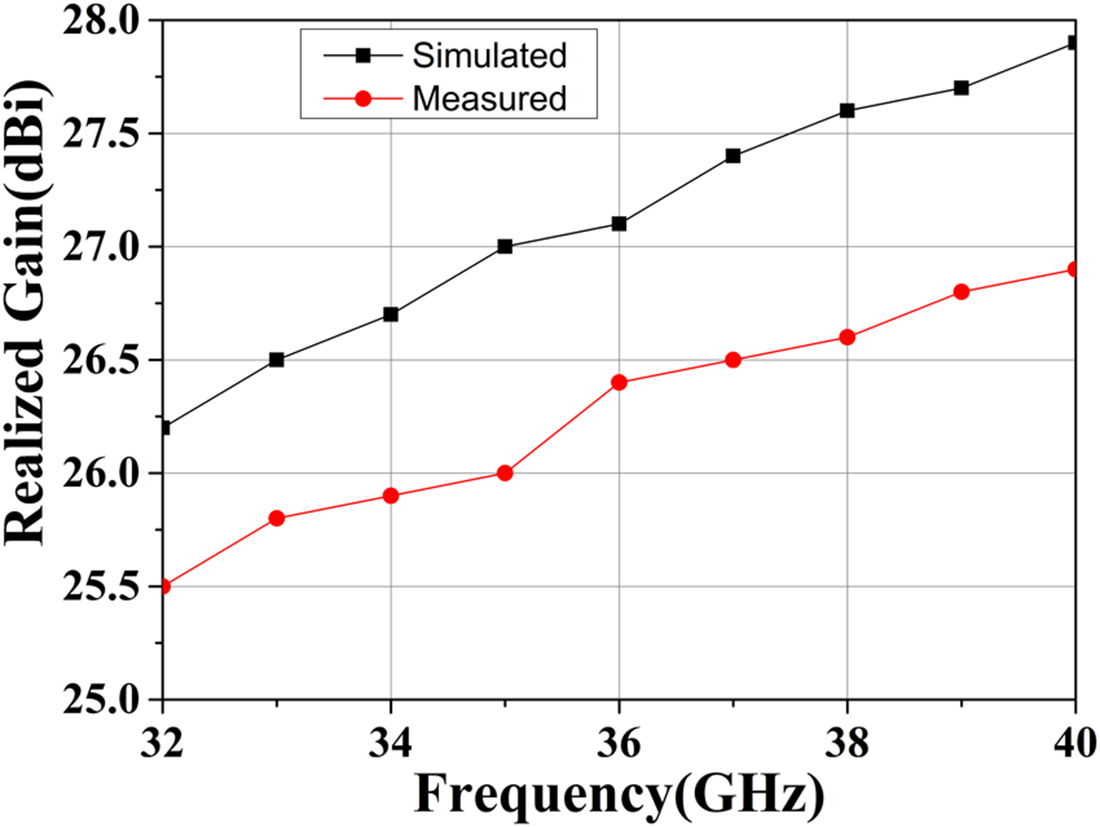
Figure 13 presents a comparison of the simulated and measured array gain. The measured values are consistently lower, with a maximum observed discrepancy of 1.1 dB. This deviation is attributed primarily to dielectric and conductor losses, as well as to amplitude and phase variations across the array elements.

Figure 13.

Measured and simulated array gain.

The measured scanning gain loss for the 28 × 6 array is presented in Table 2. The results indicate a maximum loss of 3 dB across the operating band.

Table 2.

Measured gain loss vs. scan angle (dB)

Table 2 Long description

The table reports measured antenna gain loss in decibels versus scan angle for two scan planes, azimuth and elevation, at 32, 36, and 40 GHz. In the azimuth plane, loss is higher at minus 50 degrees than at plus 50 degrees for all frequencies: 2.5 versus 2.1 dB at 32 GHz, 3.0 versus 2.9 dB at 36 GHz, and 2.1 versus 1.8 dB at 40 GHz. The maximum loss in the table is 3.0 dB at 36 GHz in the azimuth plane at minus 50 degrees. In the elevation plane, losses are much smaller and remain between 0.5 and 0.8 dB across plus 30 and minus 30 degrees. Elevation loss is slightly higher at 36 GHz than at 40 GHz, while azimuth loss peaks at 36 GHz and drops at 40 GHz. Values are limited to the listed angles and frequencies, so behavior outside these points is not shown.

Table 3 compares the performance of the proposed array with prior slant-polarized designs. References [Reference Yang, Zhang, Zhao and Zhang18, Reference Surmeli and Kizilay19], and this work employ a polarizer to achieve 45° slant polarization, whereas References [Reference Bagheri, Karlsson, Bencivenni, Gustafsson, Emanuelsson, Hasselblad and Alayón Glazunov8, Reference Keshavarz, Winson, Lipman, Abolhasan and Shariati9], and [Reference Chieh, Yeo, Kerber, Olsen, Merulla and Sharma11] utilize arrays of slant-polarized radiating elements. Although adding a polarizer increases structural complexity and profile height, it enables the array to maintain high polarization purity – specifically, a low amplitude difference between H- and V-pol components – over a wide scan range. Among polarizer-based designs, Reference [Reference Yang, Zhang, Zhao and Zhang18] offers wide bandwidth but is limited to 1D scanning with high scan loss; Reference [Reference Surmeli and Kizilay19] achieves good polarization purity but over a very narrow bandwidth and without scan analysis. Among designs using slant-polarized elements, Reference [Reference Chieh, Yeo, Kerber, Olsen, Merulla and Sharma11] attains a relatively wider scan range but suffers from high scan loss and narrow bandwidth, while Reference [Reference Bagheri, Karlsson, Bencivenni, Gustafsson, Emanuelsson, Hasselblad and Alayón Glazunov8] is outperformed by the proposed design in both bandwidth and elevation-plane scan range, and Reference [Reference Keshavarz, Winson, Lipman, Abolhasan and Shariati9], while offering wider bandwidth, provides no beam scanning analysis. Notably, to the authors’ knowledge, no similar polarizer-integrated 2D millimeter-wave phased array has been reported for practical engineering applications. The proposed array demonstrates well-balanced performance in gain, scan loss, and slant polarization purity.

Table 3.

Comparison between reported and proposed slant-polarized antenna arrays

Table 3 Long description

The table compares several slant-polarized antenna arrays by frequency range, antenna type, array size, how slant polarization is achieved, gain, two-dimensional scanning coverage, gain loss while scanning, and the maximum difference between horizontal and vertical polarization. Reported designs span from sub-gigahertz to millimeter-wave, using gap waveguide, wide-slot, patch, horn, and metal Vivaldi antennas, with arrays ranging from 1 by 4 up to 16 by 16 elements. Most prior entries use slant-polarized elements directly, while others use multi-layer polarizers, including three-layer and five-layer approaches. The proposed work operates from 32 to 40 GHz with a 28 by 6 metal Vivaldi array and a two-layer polarizer, achieving gain of at least 25.5 dBi and scanning to 50 degrees in azimuth and 30 degrees in elevation. Among entries that report scan loss, the proposed work lists about 3.0 dB loss in azimuth and 0.8 dB in elevation, which is lower than the patch array that reports 5.5 dB azimuth loss and 7.8 dB elevation loss, and lower than the horn array that reports 4.5 dB azimuth loss. Polarization imbalance is only reported for the five-layer polarizer patch (1.77 dB at broadside) and the proposed work (2.9 dB at 50 degrees azimuth and 2.5 dB at 30 degrees elevation). Several cells are marked not available, so comparisons are limited to the subset of designs that report the same metrics.