2.1. Spectrally negative Lévy processes

Recall that a spectrally negative Lévy process is a stochastic process, which has càdlàg paths and stationary and independent increments such that there are no positive discontinuities. To avoid degenerate cases in the forthcoming discussion, we shall additionally exclude from this definition the case of monotone paths. This means that we are not interested in the case of a deterministic increasing linear drift or the negative of a subordinator. Henceforth, we assume that $X=\{X_t\colon t \ge 0\}$ is a spectrally negative Lévy process defined on a probability space $ (\Omega,\mathcal{F},\mathbb{P})$ with Lévy triplet given by $ (\gamma, \sigma, \Pi)$, where $\gamma \in {\mathbb{R}}$, $\sigma\ge 0,$ and $\Pi$ is a measure concentrated on $ (0,\infty)$ satisfying

\begin{equation} \int_{(0,\infty)}(1\wedge z^2)\Pi({\rm d}z)\lt\infty.\end{equation}

The Laplace exponent of X is given by

(2.1)\begin{equation}\psi(\lambda)= \log \mathbb{E} [ {\rm{e}}^{\lambda X_1} ] = \gamma \lambda+\frac12\sigma^2\lambda^2 - \int_{(0,\infty)} ( 1-{\rm{e}}^{-\lambda z}-\lambda z\mathbf{1}_{\{0<z\leq1\}} )\Pi(\mathrm{d}z),\end{equation}

which is well defined for $\lambda\geq0$. Here $\mathbb{E}$ denotes the expectation with respect to $\mathbb{P}$. In addition, the reader should note that, for convenience, we have arranged the representation of the Laplace exponent in such a way that the support of the Lévy measure is positive even though the process experiences only negative jumps. As a strong Markov process, we shall endow X with probabilities $\{\mathbb{P}_x \colon x\in\mathbb{R}\}$ such that, under $\mathbb{P}_x,$ we have $X_0 = x$ with probability 1. Note that $\mathbb{P}_0=\mathbb{P}$ and $\mathbb{E}_0= \mathbb{E}$.

The spectrally negative Lévy process X has paths of bounded variation if and only if $\sigma=0$ and $\smash{\int_{(0,1]}z\Pi(\mathrm{d}z)} \lt \infty$, in which case, X can be written as

\begin{equation}X_t=ct-S_t, \qquad t\geq 0,\end{equation}

where $c\ :\!=\gamma+\smash{\int_{(0,1]}z\Pi(\mathrm{d}z)}$ and $\{S_t\colon t \ge 0\}$ is a drift-less subordinator. Note that we must have $c \gt 0$, since it is assumed that X does not have monotone paths.

In the classical model of the wealth of an insurance company, premium is received at a constant rate c whereas F-distributed claims arrive at the jump times of a Poisson process with rate $\mu$. The corresponding surplus process is called the Cramér–Lundberg risk process and is a special case of the spectrally negative Lévy process with $\gamma=c-\smash{\mu\int_{(0,1]}z F({\rm d} z)}$, $\sigma=0$, and $\Pi = \mu F$.

2.2. Admissible strategies

Let $D=\{ D_t\colon t \ge q 0 \}$ be a dividend strategy, meaning that it is a nonnegative and nondecreasing process adapted to the completed and right continuous filtration $\mathbb{F}\ :\!=\{\mathcal{F}_t \colon t\ge q 0\}$ of X. Here, for each fixed $t\geq0$, the quantity $D_t$ represents the cumulative dividends paid out up to time t by the insurance company whose risk process is modeled by X. The controlled Lévy process becomes $U^D=\{\smash{U^D_t}= X_t - D_t \colon t\ge q 0\}$ and we write

\begin{align}\tau^D\ :\!= \inf\{t \gt 0\colon U^D_t \lt 0 \}\end{align}

for the time at which ruin occurs when the dividend payments are taken into account.

In this work, we are interested in adding a constraint to the dividend processes. Specifically, we will only work with absolutely continuous strategies of bounded rate, i.e.

\begin{equation}D_t=\int_0^{t}d(s){{\rm{d}}}s,\qquad t\geq0,\end{equation}

such that the dividend rate d satisfies $0\leq d(t)\leq\delta$ for $t\geq0$, where $\delta>0$ is a ceiling rate. We will denote by $\Theta$ the family of admissible strategies satisfying the conditions mentioned above.

2.3. Constrained de Finetti’s problem and its dual

The expected net present value under the dividend policy $D\in\Theta$ with discounting at rate $q>0$ and initial capital $x\geq 0$ is given by

\begin{equation}v^{D}(x) = \mathbb{E}_x\bigg[\int_0^{\tau^{D}} {\rm{e}}^{-qt}\mathrm{d}D_t\bigg].\end{equation}

The dividend problem, originally considered by de Finetti, asks to maximize the expected net present value of dividend payments over the set of strategies $\Theta$.

Now, as studied in [Reference Hernández, Junca and Moreno-Franco8], we are interested in addressing a modification of this problem by adding a restriction to the dividend process D, which is given by the constraint

\begin{equation}\mathbb{E}_x[{\rm{e}}^{-q\tau^D}]\leq K,\qquad 0 \leq K\leq 1\text{ fixed.}\end{equation}

Strategies in $\Theta$ satisfying this constraint are called feasible, and are called infeasible otherwise.

We want to maximize the expected net present value of dividend payments over the set of feasible strategies. That is, we aim to solve the optimization problem, for $x\geq0$ and $0 \leq K \leq 1$,

(2.2)\begin{equation}V(x;\ K)\ :\!=\sup_{D\in\Theta}v^D(x)\quad\text{such that}\quad\mathbb{E}_x[{\rm{e}}^{-q\tau^D}]\leq K,\end{equation}

where, in the case $\smash{\mathbb{E}_x [{\rm{e}}^{-q\tau^D} ] \gt K}$ for all $D \in \Theta$, we set $V(x;\ K)= -\infty$ and call problem (2.2) infeasible.

Proceeding as in [Reference Hernández, Junca and Moreno-Franco8], we use Lagrange multipliers to reformulate the problem. For $\Lambda\geq0,$ we define the function

(2.3)\begin{equation}v_{\Lambda}^D(x;\ K)\ :\!=v^D(x)+\Lambda(K-\mathbb{E}_x[{\rm{e}}^{-q\tau^D}]).\end{equation}

Note that we can write problem (2.2) as $V(x;\ K)=\smash{\sup_{D\in\Theta}\inf_{\Lambda\geq0}v_{\Lambda}^D}(x;\ K)$ since any infeasible strategy D will make $\smash{\inf_{\Lambda\geq0}v_{\Lambda}^D(x;\ K)}=-\infty$, and any feasible strategy D will make $\smash{\inf_{\Lambda\geq0}v_{\Lambda}^D(x;\ K)=v^D_0 (x;\ K)=v^D(x)}$.

The dual problem of (2.2) is obtained by interchanging the $\sup$ with the $\inf$ in the expression above, yielding an upper bound,

(2.4)\begin{equation}V(x;\ K)=\sup_{D\in\Theta}\inf_{\Lambda\geq0}v_{\Lambda}^D(x;\ K) \leq\inf_{\Lambda\geq0} V_{\Lambda}(x;\ K),\end{equation}

where

(2.5)\begin{align}V_{\Lambda}(x;\ K)\ :\!= \sup_{D\in\Theta} v_{\Lambda}^D(x;\ K).\end{align}

Therefore, the main goal is to prove that $V(x;\ K)=\inf_{\Lambda\geq0}\displaystyle V_{\Lambda}(x;\ K)$ and to find, if it exists, an optimal $\Lambda$ (Lagrange multiplier) with which the infimum is attained. In order to do this, we will first solve (2.5).

We remark that if we set

(2.6)\begin{align}V_\Lambda(x)\ :\!=V_\Lambda(x;\ 0) \quad\textrm{and}\quad v_\Lambda^D(x) :\!=v_\Lambda^D(x;\ 0), \quad D \in \Theta,\end{align}

then $\smash{v_\Lambda^D(x;\ K) = v_\Lambda^D(x) + \Lambda K}$ and hence, $V_\Lambda(x;\ K) =V_\Lambda(x) + \Lambda K$. Therefore, solving (2.5) is equivalent to solving

(2.7)\begin{equation}V_{\Lambda}(x)\ :\!=\sup_{D\in\Theta}v_{\Lambda}^D(x).\end{equation}

4.1. Threshold strategies

The objective of this section is to show that the optimal strategies for (2.7) are of the threshold type. Under the threshold strategy $D^b$ for $b \geq 0$, the resulting controlled process $U^b$ is known as a refracted Lévy process of [Reference Kyprianou and Loeffen11], which is the unique strong solution to

$$U_t^b = {X_t} - D_t^b,\quad {\rm{where}}\quad D_t^b\;: = \delta \int_0^t {{{\mathbf{1}}_{\{ U_s^b > b\} }}} {\rm{d}}s,\quad t \ge 0.$$

Let its ruin time be

\begin{align}\tau_{b}\ :\!=\inf\{t \gt 0 \colon U^{b}_t \lt 0 \}.\end{align}

The next identities are lifted from Theorems 5(ii) and 6(ii) of [Reference Kyprianou and Loeffen11]. For $x \in \mathbb{R}$ and $b \geq 0$, we have

(4.1)\begin{align}\mathbb{E}_x\bigg[\int_0^{\tau_{b}} {\rm{e}}^{-qt} {\rm d} D^b_t\bigg]=-\delta\overline{\mathbb{W}}^{(q)}(x-b)+\frac{1}{h(b)}\biggl(W^{(q)}(x)+\delta\int_b^x {\mathbb{W}}^{(q)}(x-y)W^{(q)\prime}(y){\rm{d}}y\biggr)\end{align}

and

(4.2)\begin{align}\Psi_{x}(b)\ &:\!= \mathbb{E}_{x}[{\rm{e}}^{-q\tau_{b}}]\notag\\&=Z^{(q)}(x)+\delta q\int_b^x\mathbb{W}^{(q)}(x-y)W^{(q)}(y){\rm{d}}y\notag\\&-\frac{q\varphi(q){\rm{e}}^{\varphi(q)b}\int_b^{\infty}{\rm{e}}^{-\varphi(q)y}W^{(q)}(y) {\rm{d}}y}{h(b)} \bigg(\!W^{(q)}(x)+\delta\int_b^x\!\!\!\mathbb{W}^{(q)}(x-y)W^{(q)\prime}(y){\rm{d}}y\!\bigg),\end{align}

where

(4.3)\begin{equation}h(b)\ :\!=\varphi(q){\rm{e}}^{\varphi(q)b}\int_{b}^{\infty}{\rm{e}}^{-\varphi(q)y}W^{(q)\prime}(y){\rm{d}}y.\end{equation}

Under the threshold strategy $D^b$, the expected net present value is denoted by

(4.4)\begin{equation}v_{\Lambda}^{b}(x)\ :\!=\mathbb{E}_x\bigg[\int_0^{\tau_{b}} {\rm{e}}^{-qt} {\rm d}D^b_t\bigg]-\Lambda\Psi_{x}(b) \quad\text{for } x\geq0.\end{equation}

Using (4.1) and (4.2), we have the following result.

Proposition 4.1. The function $\smash{v_{\Lambda}^{b}}$, with $b\geq 0$, is given by

(4.5)\begin{align}v_{\Lambda}^{b}(x)&=\xi_{\Lambda}(b)\bigg(W^{(q)}(x)+\delta\int_b^x\mathbb{W}^{(q)}(x-y)W^{(q)\prime}(y){\rm{d}}y\bigg)\notag\\&-\Lambda\bigg(Z^{(q)}(x)+\delta q\int_b^x\mathbb{W}^{(q)}(x-y)W^{(q)}(y){\rm{d}}y\bigg)-\delta\overline{\mathbb W}^{(q)}(x-b) \quad\text{for $x\geq 0$,}\end{align}

where

(4.6)\begin{align}\xi_{\Lambda}(b)\ :\!=\frac{1}{h(b)}\biggl(1+ \varphi(q) q\Lambda {\rm{e}}^{\varphi(q)b}\displaystyle\int_{b}^{\infty}{\rm{e}}^{-\varphi(q)y}W^{(q)}(y) {\rm{d}}y\biggr).\end{align}

In particular, for $x \leq b$, we have

(4.7)\begin{align}v_{\Lambda}^{b}(x)=\xi_{\Lambda}(b) W^{(q)}(x) -\Lambda Z^{(q)}(x).\end{align}

Remark 4.3. From (4.3) and integration by parts,

(4.8)\begin{align}\varphi(q){\rm{e}}^{\varphi(q)b}\int_b^\infty {\rm{e}}^{-\varphi(q) y} W^{(q)} (y){\rm{d}}y = W^{(q)} (b) + \frac{h(b)}{\varphi(q)}, \qquad b \geq 0.\end{align}

Hence, the function $\xi_{\Lambda}$, given in (4.6), can be rewritten as

(4.9)\begin{equation}\xi_{\Lambda}(b)=\frac{1}{h(b)}\biggr(1+q\Lambda\bigg(W^{(q)}(b)+\frac{h(b)}{\varphi(q)}\bigg)\biggl), \qquad b \geq 0.\end{equation}

In particular, for the case $b = 0$, these expressions can be simplified as follows; the proof is deferred to Appendix A.1.

Lemma 4.1. We have

(4.10)\begin{equation}\begin{gathered}h(0)=\varphi(q) \int_{0}^{\infty}{\rm{e}}^{-\varphi(q)y}W^{(q)\prime}(y){\rm{d}}y= \varphi(q) ( - W^{(q)}(0) + \delta^{-1} ),\\\xi_{\Lambda}(0)=\frac{1}{h(0)}\biggl(1+ \frac {q \Lambda} \delta\biggr)= \dfrac{\delta+q\Lambda}{\varphi(q)(1-\delta W^{(q)}(0))},\end{gathered}\end{equation}

and, for $x\geq0$,

(4.11)\begin{align}v_{\Lambda}^{0}(x)&=\xi_{\Lambda}(0) \mathbb{W}^{(q)}(x) (1 - \delta W^{(q)}(0)) -\Lambda \mathbb{Z}^{(q)}(x) -\delta \overline{\mathbb{W}}^{(q)}(x).\end{align}

4.2. Selection of the optimal threshold $b_\Lambda$

Focusing on the set of threshold strategies, we now select our candidate optimal threshold, which we call $b_\Lambda$. In view of (4.7), such $b_\Lambda$ must maximize $\xi_\Lambda$. Motivated by this fact, we pursue $b_\Lambda$ such that $\smash{\xi'_\Lambda(b_{\Lambda})}$ vanishes if such a value exists.

First, we rewrite the form of $\smash{\xi_{\Lambda}'(b)}$ as follows. Fix $b \gt 0$. Taking a derivative in (4.9) and using the fact that $h'(b)=\varphi(q) (h(b) - \smash{W^{(q)\prime}(b)})$ (by (4.3)),

(4.12)\begin{align}\xi_{\Lambda}'(b) & = q\Lambda-\dfrac{h'(b)}{h(b)}\xi_{\Lambda}(b)\notag\\& =q\Lambda-\frac{\varphi(q)} {h(b)}\biggr(1+q\Lambda\bigg(W^{(q)}(b)+\dfrac{h(b)}{\varphi(q)}\bigg)\biggl)+\dfrac{\varphi(q)W^{(q)\prime}(b)}{h(b)}\xi_{\Lambda}(b) \notag\\& =\dfrac{\varphi(q)W^{(q)\prime}(b)}{h(b)}(\xi_{\Lambda}(b)-g_{\Lambda}(b)),\end{align}

where

(4.13)\begin{equation}g_{\Lambda}(b):\,=\dfrac{1+q\Lambda W^{(q)}(b)}{W^{(q)\prime}(b)}.\end{equation}

In view of (4.12), we now define the (candidate) optimal threshold level for (2.7) by

(4.14)\begin{equation}b_\Lambda\ :\!= \inf \{ b \gt 0\colon \xi_\Lambda'(b) \leq 0 \} = \inf \{ b \gt 0\colon \xi_\Lambda(b) - g(b) \le 0 \}.\end{equation}

Here, we set $\inf \emptyset = \infty$ for convenience, but we will see in Proposition 4.2 that $b_\Lambda$ is necessarily finite.

We will now prove an auxiliary result which describes the asymptotic behavior of the function $\xi_{\Lambda}$.

Lemma 4.2. We have

(4.15)\begin{equation}\lim_{b\to\infty}\xi_{\Lambda}(b)=\lim_{b\to\infty}g_{\Lambda}(b)=\dfrac{q\Lambda}{\Phi(q)}.\end{equation}

Proof. Recall from Remark 4.5 the convergence of $g_\Lambda$. Now, letting $b\rightarrow\infty$ in (4.9), we observe that

(4.16)\begin{equation}\lim_{b\rightarrow\infty}\xi_{\Lambda}(b)=q\Lambda\biggl(\frac{1}{\varphi(q)}+\lim_{b\rightarrow\infty}\frac{ W^{(q)}(b)}{h(b)}\biggr),\end{equation}

since $h(b)\rightarrow\infty$ as $b\rightarrow\infty$. On the other hand, by the dominated convergence theorem and using (3.7), it follows that

(4.17)\begin{align}\dfrac{W^{(q)}(b)}{h(b)} &= \biggr(\varphi(q)\int_{0}^{\infty}{\rm{e}}^{-(\varphi(q)-\Phi(q)) y} \frac {W^{(q)\prime}(y+b)} {W^{(q)}(y+b)}\dfrac{{\rm{e}}^{-\Phi(q)[y+b]}W^{(q)}(y+b)}{{\rm{e}}^{-\Phi(q)b}W^{(q)}(b)} {\rm{d}}y \biggl)^{-1}\notag\\&\xrightarrow{b \uparrow \infty} \biggl( \varphi(q)\Phi(q) \int_0^\infty {\rm{e}}^{-(\varphi(q)-\Phi(q)) y} {\rm d} y \biggr)^{-1} \nonumber\\&= \dfrac{\varphi(q)-\Phi(q)}{\varphi(q)\Phi(q)},\end{align}

where we recall that $\varphi(q)>\Phi(q)$. Now, applying (4.17) in (4.16), we get (4.15).☐

Proposition 4.2.

1. (i) Under Assumption 4.1, we have $b_{\Lambda}\in[0,a_\Lambda]$.

2. (ii) Moreover, $b_{\Lambda}=0$ if and only if one of the following two cases holds:

   1. (1) $\sigma=0$, $\Pi(0,\infty) \lt \infty$, and $\varphi(q)\geq{(\delta+q\Lambda)(q+\Pi(0,\infty))}/{(c+q\Lambda)(c-\delta)} =:\phi_1(\Lambda)$, or

   2. (2) $\sigma>0$ and $\varphi(q)\geq{2(\delta+q\Lambda)}/{\sigma^{2}} =:\phi_2(\Lambda)$.

Proof. (i) By the definition of $b_\Lambda$ as in (4.14) and the continuity of $\xi_\Lambda$ and $g_\Lambda$, in order to show that $b_\Lambda \le a_\Lambda,$ it is sufficient to show that $\xi_{\Lambda}'(b) \le 0$ (or, equivalently, $\xi_\Lambda(b) - g_\Lambda(b) \le 0$) on $[a_\Lambda,\infty)$. To show this, suppose that there exists $\bar{b} \gt a_\Lambda$ such that $\xi_\Lambda(\bar{b}) - g_\Lambda (\bar{b})> 0$. Then, since $g_{\Lambda}$ is decreasing on $ (a_\Lambda, \infty)$ as in Remark 4.5(ii), it follows by (4.12) that $\xi_\Lambda(b) - g_\Lambda(b)$ is increasing on $ (\bar{b}, \infty)$. However, this contradicts (4.15). Hence, $\xi_{\Lambda}'(b) \le 0$ on $[a_\Lambda, \infty)$.

(ii) Using (4.12) and the definition of $b_{\Lambda}$ given in (4.14), we obtain $b_{\Lambda}=0$ if and only if $g_{\Lambda}(0+)\geq \xi_{\Lambda}(0+)$. This is equivalent, by Lemma 4.1 and Remark 4.5(i), to

$$\varphi \left( q \right) \ge {{\left( {\delta + q\Lambda } \right){W^{\left( q \right)'}}\left( {0 + } \right)} \over {\left( {1 + q\Lambda {W^{\left( q \right)}}\left( 0 \right)} \right)\left( {1 - \delta {W^{\left( q \right)}}\left( 0 \right)} \right)}}.$$

From here, using (3.5) and (3.6), we obtain the two cases announced in the proposition.

4.3. Verification

For the case $b_\Lambda \gt 0$, by how $b_\Lambda$ is selected as in (4.14), together with (4.5) and (4.12), we can write

(4.18)\begin{align}\begin{split}v_{\Lambda}^{b_\Lambda}(x) &= g_{\Lambda}(b_\Lambda)\bigg(W^{(q)}(x)+\delta\int_{b_\Lambda}^x\mathbb{W}^{(q)}(x-y)W^{(q)\prime}(y){\rm{d}}y\bigg)\\& -\Lambda\bigg(Z^{(q)}(x)+\delta q\int_{b_\Lambda}^x\mathbb{W}^{(q)}(x-y)W^{(q)}(y){\rm{d}}y\bigg)-\delta\overline{\mathbb W}^{(q)}(x-b_\Lambda) \quad\text{for$x\geq 0$.}\end{split}\end{align}

For the case $b_\Lambda = 0$, the function $\smash{v_{\Lambda}^{b_\Lambda} \equiv v_{\Lambda}^{0}}$ is given in (4.11).

Given the spectrally negative Lévy process X, we call a function $F\colon \mathbb{R} \to \mathbb{R}$ sufficiently smooth if F is continuously differentiable on $ (0,\infty)$ when X has paths of bounded variation and is twice continuously differentiable on $ (0,\infty)$ when X has paths of unbounded variation. We let $\Gamma$ be the operator acting on a sufficiently smooth function F, defined by

\begin{equation}\Gamma F(x)\ :\!= \gamma F'(x)+\frac{\sigma^2}{2}F''(x)+\int_{(0,\infty)}(F(x-z)-F(x)+F'(x)z\mathbf{1}_{\{0 \lt z\le 1\}})\Pi(\mathrm{d}z), \qquad x \gt 0.\end{equation}

The following lemma constitutes standard technology as far as optimal control is concerned. For its proof we refer the reader to that of Lemma 1 in [Reference Loeffen14].

Lemma 4.3. Suppose that $\smash{\hat{D}\in\Theta}$ is an admissible dividend strategy such that $\smash{v^{\hat{D}}_{\Lambda}}$ is sufficiently smooth on ($0,\infty$), $\smash{v_\Lambda^{\hat{D}}(0)}\geq -\Lambda$, and, for all $x \gt 0$,

(4.19)\begin{equation}(\Gamma -q) v^{\hat{D}}_{\Lambda}(x)+\sup_{0\le r\le \delta}(r-rv^{\hat{D}\prime}_{\Lambda}(x))\le 0.\end{equation}

Then $\smash{v^{\hat{D}}_{\Lambda}(x)}=V_{\Lambda}(x)$ for all $x\geq0$ and hence, $\smash{\hat{D}}$ is an optimal strategy.

We first show that our candidate value function $\smash{v^{b_{\Lambda}}_{\Lambda}}$ is indeed sufficiently smooth on $ (0,\infty)$. The proof is given in Appendix A.2.

Lemma 4.5. The value function $\smash{v^{b_{\Lambda}}_{\Lambda}}$ satisfies (4.19) if and only if

(4.20)\begin{equation}v^{b_{\Lambda}\prime}_{\Lambda}(x)\geq1 \quad\text{if $0<x\le b_{\Lambda}$}, \qquad v^{b_{\Lambda}\prime}_{\Lambda}(x)\le 1 \quad\text{if$x>b_{\Lambda}$}.\end{equation}

We now state the main theorem of this section. Its proof is provided in Appendix A.3.1.

6.1. Scale functions under a change of measure

For each $ \beta \ge 0$, we define the change of measure

\begin{equation}\dfrac{{\rm d}\tilde{\mathbb{P}}^{\beta}_{x}}{{\rm d}\tilde{\mathbb{P}}_{x}}\biggr|_{\mathcal{F}_{t}}={\rm{e}}^{\beta(Y_{t}-x)-\psi_Y(\beta)t}, \qquad x\in\mathbb{R}, \, t\geq0,\end{equation}

where $\smash{\tilde{\mathbb{P}}_x}$ is the law of the process Y when it starts at x. It is known that Y is still a spectrally negative Lévy process on $ (\Omega, \mathcal{F},\smash{\tilde{\mathbb{P}}^{\beta}})$ and the scale function of Y on this probability space can be written

\begin{gather}\mathbb{W}_{ \beta }^{(u-\psi_Y( \beta ))}(x)={\rm{e}}^{-\beta x}\mathbb{W}^{(u)}(x),\\\mathbb{Z}_{ \beta}^{(u-\psi_{Y}(\beta))}(x)=1+(u-\psi_Y( \beta))\int_{0}^{x}{\rm{e}}^{- \beta z}\mathbb{W}^{(u)}(z) {\rm{d}}z,\end{gather}

with $u-\psi_Y( \beta)\geq0$; see [2, Remark 4]. In particular, (3.1) and (3.3) give $q-\psi_{Y}(\Phi(q))=\delta\Phi(q)$ and hence,

(6.1)\begin{align}\mathbb{W}^{(\delta\Phi(q))}_{\Phi(q)}(x)={\rm{e}}^{-\Phi(q)x}\mathbb{W}^{(q)}(x) \quad\text{and}\quad\mathbb{Z}^{(\delta\Phi(q))}_{\Phi(q)}(x)=1+\delta\Phi(q)\int_{0}^{x}{\rm{e}}^{-\Phi(q)z}\mathbb{W}^{(q)}(z){\rm{d}}z.\end{align}

6.2. Optimal dividend problem with terminal value

As in the case of the spectrally negative Lévy process, we are first interested in solving problem (2.4) for the spectrally positive case. For this purpose, first we need to study the optimal dividend problem with a terminal value for the process $\overline{Y}$. Using Theorems 5(i) and 6(iii) of [Reference Kyprianou and Loeffen11] we have the following result, whose proof is deferred to Appendix A.7.

Proposition 6.1. For $x,b,q\geq0$, we have

(6.2)\begin{equation}\overline{\Psi}_{x}(b)\ :\!=\overline{\mathbb{E}}_x[{\rm{e}}^{-q\bar{\tau}_{b}};\bar{\tau}_{b} \lt \infty]={\rm{e}}^{-\Phi(q)x}\frac{\mathbb{Z}^{(\delta\Phi(q))}_{\Phi(q)}(b-x)}{\mathbb{Z}^{(\delta\Phi(q))}_{\Phi(q)}(b)},\end{equation}

where $\mathbb{Z}^{(\delta\Phi(q))}_{\Phi(q)}(x)$ is given in (6.1), $\bar{\tau}_{b}\ :\!=\inf\{ t \gt 0\colon \overline{U}^b_t=0\},$ and

(6.3)\begin{equation}\overline{\mathbb{E}}_x\biggr[ \int_0^{\bar{\tau}_{b}} {\rm{e}}^{-qt}{\rm d}\overline{D}^{b}_{t}\biggl] =\dfrac{\delta}{q}(\mathbb{Z}^{(q)}(b-x)-\mathbb{Z}^{(q)}(b)\overline{\Psi}_{x}(b)).\end{equation}

Using (6.2) and (6.3), we have the following result.

Proposition 6.2. For $b \geq 0$, we have

(6.4)\begin{equation}\bar{v}_{\Lambda}^{b}(x)\ :\!=\overline{\mathbb{E}}_x\bigg[\int_0^{\bar{\tau}_{b}}{\rm{e}}^{-qt}{\rm d} \overline{D}^b_t\bigg]- \Lambda \overline{\Psi}_{x}(b) =\begin{cases}\displaystyle{\frac{\delta}{q}\mathbb{Z}^{(q)}(b-x)-\bar{k}_{x}(b,\Lambda)}&\text{if}\ 0 \le x\le b,\\[9pt]\displaystyle{\frac{\delta}{q}-\bar{k}_{b}(b,\Lambda){\rm{e}}^{-\Phi(q)(x-b)}}&\text{if}\ x>b,\end{cases}\end{equation}

where, for $x\geq0$,

\begin{align}\bar{k}_{x}(b,\Lambda)\ & :\!=\overline{\Psi}_{x}(b)\biggr(\dfrac{\delta}{q}\mathbb{Z}^{(q)}(b)+\Lambda\biggl).\end{align}

In order to select the optimal threshold, we apply smooth fit. Note that, by (6.4), $\bar{v}_{\Lambda}^{b}$ is continuous on $[0,\infty)$ for any choice of b. Here, we will study the smoothness of $\smash{\bar{v}_{\Lambda}^{b}}$ at $x=b$ to propose a candidate threshold level $\smash{\bar{b}_{\Lambda}}$ such that $\smash{\bar{v}_{\Lambda}^{\bar{b}_{\Lambda}}}$ is ${\rm{C}}^{1}(0,\infty)$ and ${\rm{C}}^{2}(0,\infty)$ when $\overline{Y}$ is of bounded and unbounded variation, respectively. By differentiating (6.4), we see that

(6.5)\begin{equation}\bar{v}_{\Lambda}^{b\prime}(x)=\begin{cases}-\delta\mathbb{W}^{(q)}(b-x)+\Phi(q) (\bar{k}_{x}( b ,\Lambda)+\delta\bar{k}_{b}(b,\Lambda)\mathbb{W}^{(q)}(b-x)) &\text{if}\ 0 \lt x \lt b,\\\Phi(q)\bar{k}_{b}(b,\Lambda){\rm{e}}^{-\Phi(q)(x-b)} &\text{if}\ x>b,\end{cases}\end{equation}

and, in particular, for the unbounded variation case

(6.6)\begin{equation}\bar{v}_{\Lambda}^{b\prime\prime}(x)=\begin{cases}\delta\mathbb{W}^{(q)\prime}(b-x)-[\Phi(q)]^{2} \bar{k}_{x}( b ,\Lambda)&\\\quad-\delta\Phi(q)\bar{k}_{b}(b,\Lambda)[\Phi(q)\mathbb{W}^{(q)}(b-x)+\mathbb{W}^{(q)\prime}(b-x)] &\text{if}\ 0< x<b,\\-[\Phi(q)]^{2}\bar{k}_{b}(b,\Lambda){\rm{e}}^{-\Phi(q)(x-b)} &\text{if}\ x>b,\end{cases}\end{equation}

where we recall that, if Y is of unbounded variation, $\smash{\mathbb{W}^{(q)}}$ is ${C}^{1}$ on $ (0,\infty)$. From (6.5) and (6.6), together with (3.5) and (3.6), we have the following result.

Lemma 6.1. Suppose that $b \gt 0$ is such that

(6.7)\begin{equation}\bar{k}_{b}(b,\Lambda)=\dfrac{1}{\Phi(q)}, \quad\text{or,equivalently,}\quad \Lambda {\rm{e}}^{-\Phi(q)b} = s(b),\end{equation}

where

(6.8)\begin{equation}s(b)\ :\!=\frac{1}{\Phi(q)}\mathbb{Z}^{(\delta\Phi(q))}_{\Phi(q)}(b)-\dfrac{\delta {\rm{e}}^{-\Phi(q)b}}{q}\mathbb{Z}^{(q)}(b), \qquad b> 0.\end{equation}

Then, the function $\smash{\bar{v}_{\Lambda}^{b}}$ is $C^1(0, \infty)$ and $C^2(0, \infty)$ for the case of bounded and unbounded variation, respectively.

Lemma 6.2. If $\Lambda>{1}/{\Phi(q)}-{\delta}/{q}$, then there exists a unique $b>0$ that satisfies (6.7).

Proof. In order to prove the lemma, we will show that s(b) as in (6.8) is strictly increasing and satisfies

(6.9)\begin{equation}\displaystyle\lim_{b\rightarrow0}s(b)=\dfrac{1}{\Phi(q)}-\dfrac{\delta}{q} \quad\text{and}\quad \lim_{b\rightarrow\infty}s(b)=\infty.\end{equation}

1. (i) Since $s'(b)=\smash{{\delta\Phi(q){\rm{e}}^{-\Phi(q)b}\mathbb{Z}^{(q)}(b)}/{q}}>0$ for all $b \gt 0$, then $s(\cdot)$ is strictly increasing on $ (0,\infty)$.

2. (ii) Letting $b\rightarrow0$ in (6.8), it is easy to see that the first limit of (6.9) holds.

3. (iii) Note that

(6.10)\begin{equation}s(b)=\frac{\delta\mathbb{Z}^{(q)}(b)}{q\Phi(q){\rm{e}}^{\Phi(q)b}}\biggr(\dfrac{q{\rm{e}}^{\Phi(q)b}\mathbb{Z}^{(\delta\Phi(q))}_{\Phi(q)}(b)}{\delta\mathbb{Z}^{(q)}(b)}-\Phi(q)\biggl).\end{equation}

Using l’Hôpital’s rule, (3.7), and the fact that $\varphi(q)> \Phi(q)$, the following limits can be verified:

\begin{gather*}\lim_{b\rightarrow\infty}\dfrac{\mathbb{Z}^{(q)}(b)}{{\rm{e}}^{\Phi(q)b}}=\lim_{b\rightarrow\infty}q[\Phi(q)]^{-1}{\rm{e}}^{(\varphi(q)-\Phi(q))b}{\rm{e}}^{-\varphi(q)b}\mathbb{W}^{(q)}(b)=\infty,\\[4pt]\lim_{b\rightarrow\infty}\dfrac{\mathbb{Z}^{(\delta\Phi(q))}_{\Phi(q)}(b)}{{\rm{e}}^{(\varphi(q)-\Phi(q))b}}=\lim_{b\rightarrow\infty}\delta\Phi(q)\dfrac{{\rm{e}}^{-\varphi(q)b}\mathbb{W}^{(q)}(b)}{\varphi(q)-\Phi(q)}=\delta\Phi(q)\dfrac{\psi'_{Y}(\varphi(q))^{-1}}{\varphi(q)-\Phi(q)},\\[4pt]\begin{aligned}\lim_{b\rightarrow\infty}\dfrac{q{\rm{e}}^{\Phi(q)b}\mathbb{Z}^{(\delta\Phi(q))}_{\Phi(q)}(b)}{\delta\mathbb{Z}^{(q)}(b)}&=\lim_{b\rightarrow\infty}\dfrac{\Phi(q)({\mathbb{Z}^{(\delta\Phi(q))}_{\Phi(q)}(b)}/{\delta {\rm{e}}^{(\varphi(q)-\Phi(q))b}}+{\rm{e}}^{-\varphi(q)b}\mathbb{W}^{(q)}(b))}{{\rm{e}}^{-\varphi(q)b}\mathbb{W}^{(q)}(b)}\\[4pt]&=\Phi(q)\bigg(1+\dfrac{\Phi(q)}{\varphi(q)-\Phi(q)}\biggr).\end{aligned}\end{gather*}

Hence, it follows that $ \lim_{b\to\infty}s(b)=\infty$.☐

Now, we let $\bar{b}_\Lambda$ be as in Lemma 6.2 for the case $\Lambda>{1}/{\Phi(q)}-{\delta}/{q}$ and set it to 0 otherwise.

1. (i) When $\Lambda>{1}/{\Phi(q)}-{\delta}/{q}$, applying (6.7) in (6.4), with $b=\bar{b}_\Lambda$, we see that $\smash{\bar{v}_{\Lambda}^{\bar{b}_\Lambda}}$ is given by

   (6.11)\begin{equation}\bar{v}_{\Lambda}^{\bar{b}_\Lambda}(x)=\begin{cases}\displaystyle{\frac{\delta}{q}\mathbb{Z}^{(q)}(\bar{b}_\Lambda-x)-\frac{{\rm{e}}^{-\Phi(q)(x-\bar{b}_\Lambda)}}{\Phi(q)}\mathbb{Z}^{(\delta\Phi(q))}_{\Phi(q)}(\bar{b}_\Lambda-x)} &\text{if}\ x\le\bar{b}_\Lambda,\\[5pt]\displaystyle{\frac{\delta}{q}-\frac{{\rm{e}}^{-\Phi(q)(x-\bar{b}_\Lambda)}}{\Phi(q)}}&\text{if}\ x>\bar{b}_\Lambda.\end{cases}\end{equation}

2. (ii) When $\Lambda\le{1}/{\Phi(q)}-{\delta}/{q}$, using (6.4) and because $\bar{k}_0(0, \Lambda)={\delta}/{q}+\Lambda$, we have

   (6.12)\begin{align}\bar{v}^{0}_{\Lambda}(x)=\dfrac{\delta}{q}-{\rm{e}}^{-\Phi(q)x}\bigg(\dfrac{\delta}{q}+\Lambda\bigg), \qquad x \geq 0.\end{align}

6.3. Constrained de Finetti’s problem for spectrally positive Lévy processes

Now we consider problem (2.2) driven by the spectrally positive Lévy process $\overline{Y}$. Note that ${\overline{D}^{\bar{b}_\Lambda}}$ is the optimal strategy for (2.5) for any $K\in[0,1]$.

Let us define $\tilde{\Lambda}\ :\!={1}/{\Phi(q)}-{\delta}/{q}$. Following Lemma 6.2, if $\tilde{\Lambda}\geq0,$ we have $\bar{b}_{\Lambda}=0$ for $\Lambda\in[0,\tilde{\Lambda}]$; on the other hand, if $\tilde{\Lambda}<0$ then $\bar{b}_{\Lambda}>0$ for all $\Lambda \gt 0$.

Similarly to Section 5, we need to establish the relationship between $\Lambda$ and its corresponding threshold level $\bar{b}_\Lambda$ given by Lemma 6.2. From (6.7) we obtain $\Lambda =\tilde{\lambda}(\bar{b}_\Lambda)$ for $\Lambda \gt \tilde{\Lambda},$ where

\begin{equation}\tilde{\lambda}(b) ={\rm{e}}^{\Phi(q)b} s(b),\end{equation}

with s defined in (6.10). Since s is strictly increasing (see the proof of Lemma 6.2) and satisfies (6.9), it immediately follows that $ \tilde{\lambda}$ is also strictly increasing, $\lim_{b\rightarrow\infty} \tilde{\lambda}(b)=\infty,$ and

\begin{equation}\lim_{b\rightarrow \bar{b}_{0}} \tilde{\lambda}(b)=\begin{cases}\displaystyle{\frac{1}{\Phi(q)}-\frac{\delta}{q}} &\text{if}\ \bar{b}_{0}=0,\\0 &\text{if}\ \bar{b}_{0}>0.\end{cases}\end{equation}

Here, the convergence for the case $\bar{b}_{0} \gt 0$ holds by the fact that

[$$\mathop {\lim }\limits_{b \to {{\overline b }_0}} \overline \lambda \left( b \right) = \mathop {\lim }\limits_{b \to {{\overline b }_0}} {{\rm{e}}^{\phi \left( q \right)b}}s\left( b \right) = {{\rm{e}}^{\phi \left( q \right){{\overline b }_0}s\left( {\overline {{b_0}} } \right)}} = 0,$$

where the last equality follows because (6.7) and Lemma 6.2 imply that $s(\bar{b}_{0}) = 0$. Note that $\smash{\bar{b}_{\tilde{\lambda}(b)}}=b$ for all $b>\bar{b}_{0}$.

Next, we need to show that the function $b\mapsto\overline{\Psi}_{x}(b)$, given in (6.2), is strictly decreasing with $x>0$ fixed. In the case that $x=0$, we see that $\overline{\Psi}_{0}(b)=1$ by (6.2). The proof of the following lemma is given in Appendix A.8.

Lemma 6.3. Let $x \gt 0$ be fixed. Then the function $b \mapsto \overline{\Psi}_{x}(b)$ defined in (6.2) is strictly decreasing and satisfies

\begin{equation}\lim_{b\rightarrow0}\overline{\Psi}_{x}(b)={\rm{e}}^{-\Phi(q)x}\quad\text{and}\quad \lim_{b\rightarrow\infty}\overline{\Psi}_{x}(b)={\rm{e}}^{-\varphi(q)x}.\end{equation}

Finally, using similar arguments as in Theorem 5.1 (noting that we have results analogous to Lemmas 5.1(iv) and 5.2), we obtain the following theorem.

Theorem 6.2. Let $x \gt 0$ be fixed. Then

\begin{equation}\bar{v}(x;\ K)=\begin{cases}\bar{v}^{\bar{b}_0}_{0}(x;\ K) &\text{if}\ K \in[\overline{\Psi}_{x}(\bar{b}_0),1],\\\inf_{\Lambda\geq0} \bar{v}_{\Lambda}(x;\ K) &\text{if}\ K\in({\rm{e}}^{-\varphi(q)x},\overline{\Psi}_{x}(\bar{b}_0)),\\0 &\text{if}\ K={\rm{e}}^{-\varphi(q)x},\\-\infty &\text{if}\ K \in[0,{\rm{e}}^{-\varphi(q)x}).\end{cases}\end{equation}

7.1. Spectrally negative case

We first consider the spectrally negative case as studied in Sections 4 and 5. Here we assume that X is of the form

(7.1)\begin{equation}X_t - X_0= c t+ 0.2 B_t - \sum_{n=1}^{N_t} Z_n, \qquad 0\le t \lt \infty,\end{equation}

where $B=\{B_t \colon t\ge 0\}$ is a standard Brownian motion, $N=\{N_t\colon t\ge 0\}$ is a Poisson process with arrival rate $\kappa$, and $Z=\{Z_n;\ n = 1,2,\ldots\}$ is an i.i.d. sequence of exponential variables with parameter 1 (so that Assumption 4.1 is satisfied). Here, the processes B, N, and Z are assumed mutually independent. We refer the reader to [Reference Egami and Yamazaki5] and [Reference Kuznetsov, Kyprianou and Rivero9] for the forms of the corresponding scale functions.

We consider the following two parameter sets.

Case 1: $\kappa = 1$, $\sigma = 0.2$, $c = 1.5$, $\delta = 1$.

Case 2: $\kappa = 0.01$, $\sigma = 0$, $c = 5$, $\delta = 0.1$.

Here, case 2 corresponds to the case $\bar{\Lambda} = \infty$ where we have $b_\Lambda = 0$ for any choice of $\Lambda$ as in Remark 4.6.

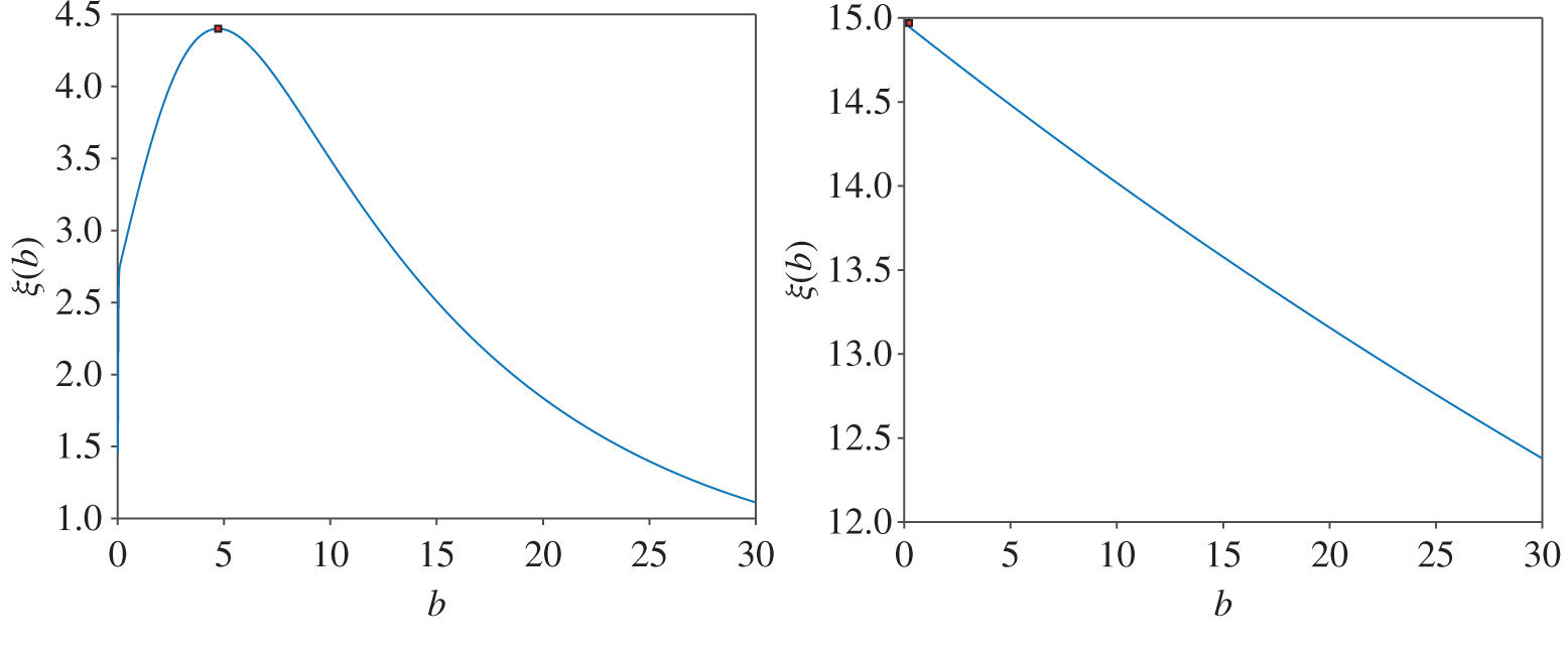
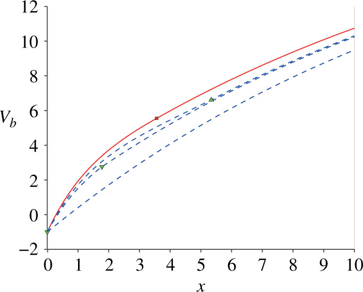
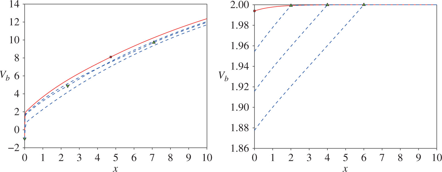
We first show the optimal solutions for the problem considered in Section 4 focusing on the case $\Lambda = 1$. In Figure 1 we plot the function $b \mapsto \xi_\Lambda(b)$ as in (4.6) and (4.9). Here, in case 1, it attains a global maximum and the maximizer becomes $b_\Lambda$ by (4.14). In contrast, in case 2, it is monotonically decreasing and, by (4.14), we have $b_\Lambda = 0$. In Figure 2, we plot the optimal value function $x \mapsto V_\Lambda(x) =v_\Lambda^{b_\Lambda}(x)$ along with the suboptimal value functions $v_\Lambda^{b}$ for the choice of $b = 0, \bar{b}_\Lambda/2, 3\bar{b}_\Lambda/2$ for case 1 and $b = 2,4,6$ for case 2. In both cases, we confirm that $V_\Lambda$ dominates the suboptimal ones uniformly in x.

Figure 1:

Plots $b \mapsto \xi_\Lambda(b)$ for case 1 (left) and case 2 (right). The points at $b_\Lambda$ are indicated by squares.

Figure 2:

Plots of $x \mapsto V_\Lambda(x)$ (solid lines) for case 1 (left) and case 2 (right). Suboptimal value functions $v_\Lambda^{b}$ (dotted lines) are also plotted for the choice of $b = 0, \bar{b}_\Lambda/2, 3 \bar{b}_\Lambda/2$ for case 1 and $b =2,4,6$ for case 2. The points at $b_\Lambda$ are indicated by squares and those at b in the suboptimal cases are indicated by up- (respectively down-) pointing triangles when $b \gt b_\Lambda$ (respectively $b \lt b_\Lambda$).

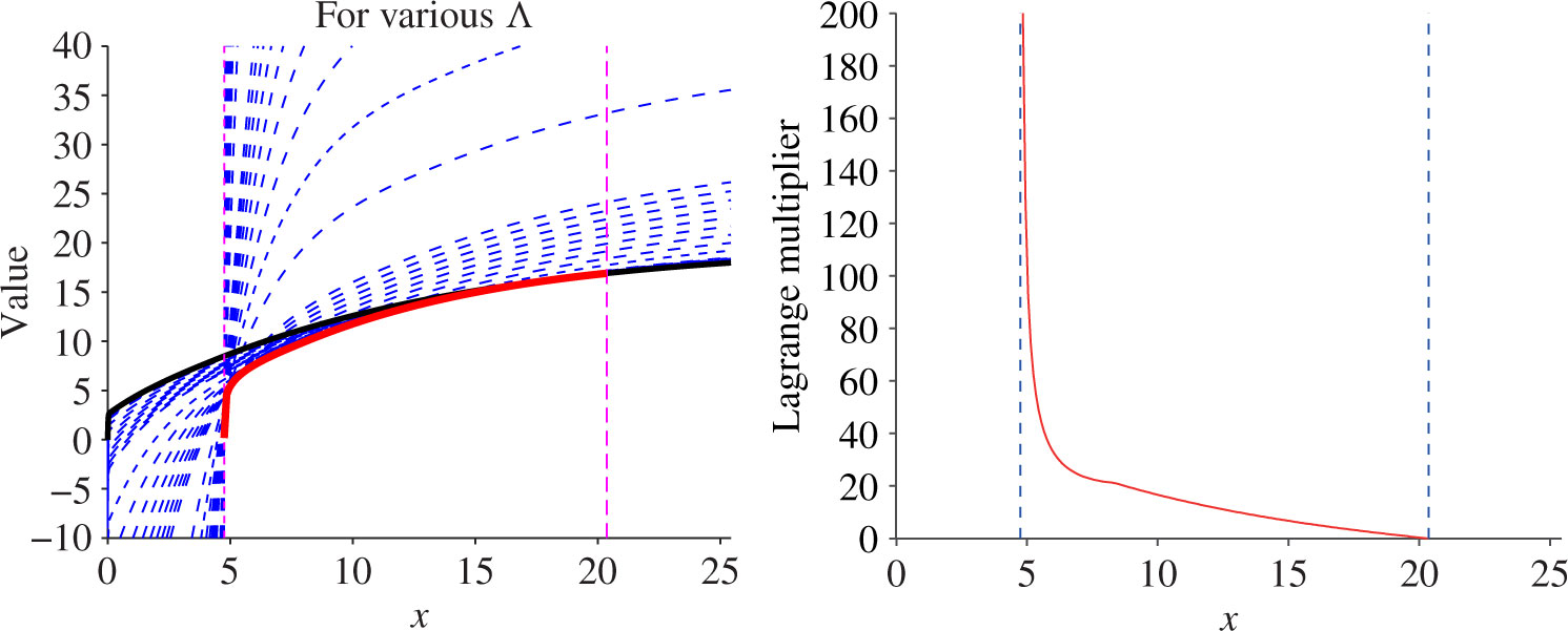
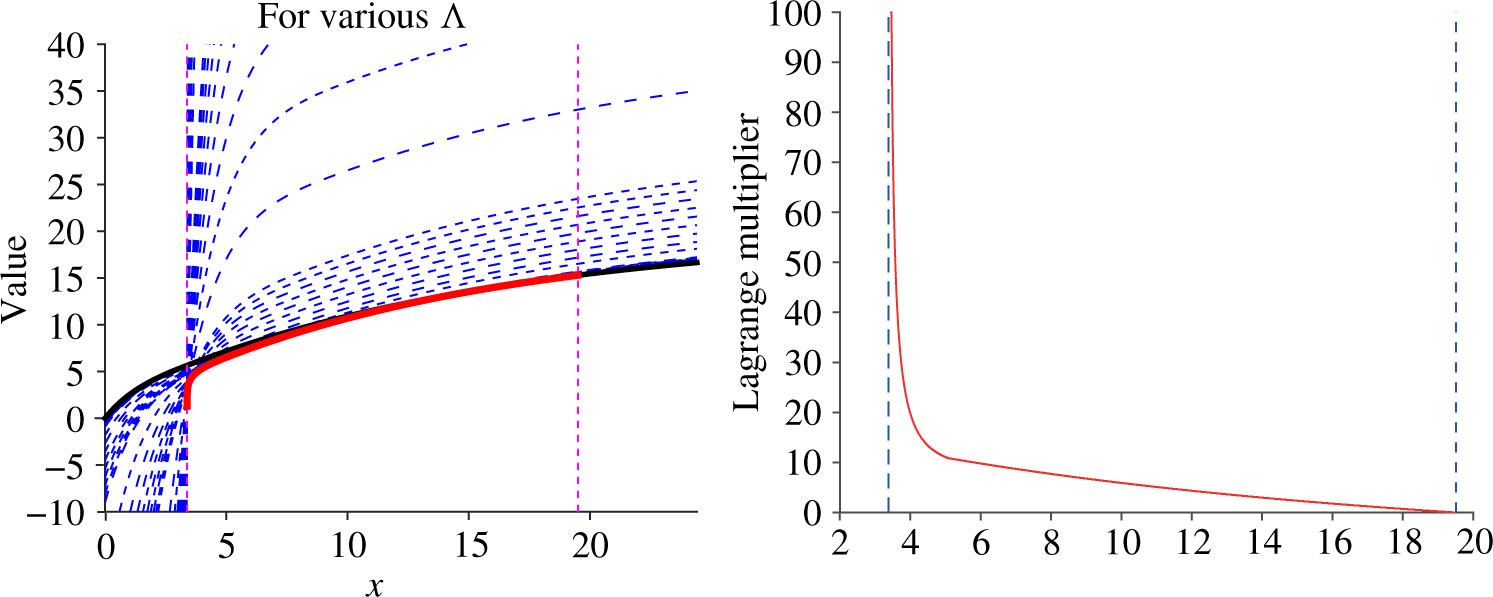
We now move onto the constrained problem (2.2) studied in Section 5, focusing on case 1 with $K = 0.1$. Recall that the optimal solutions are given in Theorem 5.1. In the left-hand panel of Figure 3, we plot the function $x \mapsto V_\Lambda(x;\ K) = V_\Lambda(x) + \Lambda K$ for various values of $\Lambda$ ranging from 0 to $20\,000$. For $x \in (\underline{x},\overline{x}),$ where $\underline{x}$ and $\overline{x}$ are such that $K_{\underline{x}} = K$ and $\Psi_{\overline{x}}(b_0) = K$, respectively, its minimum over the considered $\Lambda$ gives (an approximation of) $V(x;\ K)$, indicated by the solid red line in the plot. On the other hand, $V(x;\ K)$ equals $V_0(x;\ K) = v_0^{b_0}(x;\ K)$ for $x \in[\overline{x},\infty)$ and it is infeasible for $x \in[0,\underline{x})$. In the right-hand panel of Figure 3, we plot, for $x \in (\underline{x},\overline{x})$, the Lagrange multiplier $\Lambda^* :\,= \arg \min_{\Lambda\geq 0} V_\Lambda(x;\ K)$. We observe that $\Lambda^*$ goes to $\infty$ as $x \downarrow \underline{x}$ and to 0 as $x \uparrow \overline{x}$.

Figure 3:

(Left) Plots of $x \mapsto V_\Lambda(x;\ K)$ for $\Lambda = 0.1$, $\ldots$, 1, 2, $\ldots$, 10, 20, $\ldots$, 100, 200, $\ldots$, 1000, 2000, $\ldots$, $10\,000$, $20\,000$ (dotted lines) and for $\Lambda = 0$ (solid, boldface line) for the case $K = 0.1$. The two vertical dotted lines indicate the values of $\underline{x}$ and $\overline{x}$ such that $K_{\underline{x}} = K$ and $\Psi_{\overline{x}}(b_0) = K$. On $[\underline{x}, \overline{x}]$, the minimum of $V_\Lambda(x;\ K)$ over $\Lambda$ is shown by a solid boldface red line. (Right) Plots of the Lagrange multiplier $\Lambda^*$ on $ (\underline{x}, \overline{x}]$ with the same two vertical lines as in the left plot.

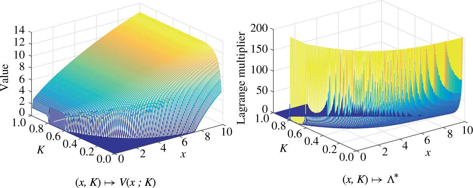
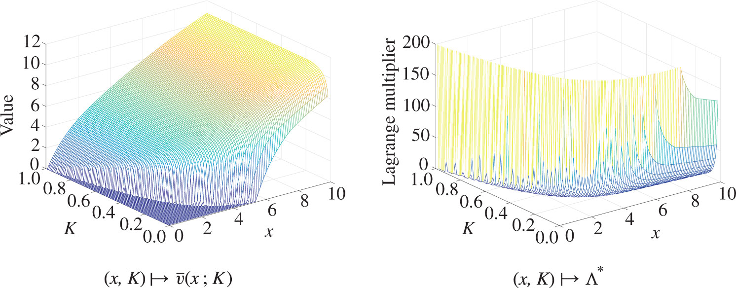
In Figure 4, we show the values of $V(x;\ K)$ and the Lagrange multiplier $\Lambda^*$ as functions of $ (x\ ,\ K)$. Here, those $ (x\ ,\ K)$ at which the problem is infeasible are indicated by dark shades on the $z = 0$ plane. It is confirmed that $V(x;\ K)$ increases as x and K increase, while $\Lambda^*$ increases as $ (x\ ,\ K)$ decrease.

Figure 4:

Plots of $V(x;\ K)$ (left) and the Lagrange multiplier $\Lambda^*$ (right) as functions of x and K.

7.2. Spectrally positive case

Similarly, we confirm the results in Section 6 focusing on the case $\overline{Y}$ is of the form

[$$\matrix{ {\overline {{Y_t}} - \overline {{Y_0}} = - t + 0.2{B_t} + \sum\limits_{n = 1}^{{N_t}} {{Z_n}} } & {{\rm{for }}t \ge 0.} \cr } $$

Here B and N (with $\kappa = 1.5$) are the same as in the case of (7.1), and Z is a phase-type random variable that approximates the Weibull distribution with shape parameter 2 and scale parameter 1 (see [Reference Avanzi, Pérez, Wong and Yamazaki1] for the parameters of the phase-type distribution). Throughout, we set $\delta = 1$.

For the (Lagrangian) problem considered in Section 6.2, the optimal threshold $\smash{\bar{b}_\Lambda}$ is such that (6.7) holds and the value function $\smash{\bar{v}_\Lambda(x) =\bar{v}_\Lambda^{\bar{b}_\Lambda}(x)}$ is given in (6.11). In Figure 5 we plot the optimal value function $x\mapsto \bar{v}_\Lambda(x)$ along with suboptimal value functions $\bar{v}_\Lambda^{b}$ for the choice of $b = 0, \bar{b}_\Lambda/2, 3\bar{b}_\Lambda/2$ when $\Lambda = 1$. For the constrained case considered in Section 6.3, in Figures 6 and 7, we plot analogous results to those shown in Figures 3 and 4, where we assume that $K =0.1$ for Figure 6. It is confirmed that similar behaviors of the value function and the Lagrange multiplier can be observed as in the spectrally negative case.

Figure 5:

Plots of $x \mapsto \bar{v}_\Lambda(x)$ along with suboptimal value functions $\bar{v}_\Lambda^{b}$ (dotted lines) for the choice of $b= 0, \bar{b}_\Lambda/2, 3 \bar{b}_\Lambda/2$. The point at $\bar{b}_\Lambda$ is indicated by a square and the points at b in the suboptimal cases are indicated by up- (respectively down-) pointing triangles when $b \gt \bar{b}_\Lambda$ (respectively $b \lt \bar{b}_\Lambda$).

Figure 6:

(Left) Plots of $x \mapsto \bar{v}_\Lambda(x;\ K)$ for $\Lambda = 0.1$, $\ldots$, 1, 2, $\ldots$, 10, 20, $\ldots$, 100, 200, $\ldots$, 1000, 2000, $\ldots$, $10\,000$, $20\,000$ (dotted lines) and for $\Lambda = 0$ (solid, boldface line) for the case $K = 0.1$. The two vertical dotted lines indicate the values of $\underline{x}$ and $\overline{x}$ such that $\exp (- \varphi(q)\underline{x})= K$ and $\overline{\Psi}_{\overline{x}}(\bar{b}_0) = K$. On $[\underline{x}, \overline{x}]$, the minimum of $\bar{v}_\Lambda(x;\ K)$ over $\Lambda$ is shown by the solid boldface red line. (Right) Plots of the Lagrange multiplier $\Lambda^*$ on $ (\underline{x},\overline{x}]$ with the same two vertical lines as in the left plot.

Figure 7:

Plots of $\bar{v}(x;\ K)$ (left) and the Lagrange multiplier $\Lambda^*$ (right) as functions of x and K