1 Introduction
Engineering applications such as micro air vehicles and energy harvesting are designed to mimic the propulsive flapping mechanism of swimming and flying animals, although these applications are less efficient. The early research on propulsive flapping of swimming animals by Triantafyllou, Triantafyllou & Gopalkrishnan (Reference Triantafyllou, Triantafyllou and Gopalkrishnan1991) and Triantafyllou, Triantafyllou & GrosenBaugh (Reference Triantafyllou, Triantafyllou and GrosenBaugh1993) set a range for effective Strouhal numbers ( $St_{A}=2Af/U$, where
 $A$ is the trailing-edge amplitude,
 $f$ is the flapping frequency and
 $U$ is the free-stream velocity) as 0.25–0.35, but it was argued only for large-aspect-ratio (AR) tails (Rohr & Fish Reference Rohr and Fish2004; Eloy Reference Eloy2012). Nevertheless, flapping foil research primarily focuses on
 $St_{A}=0.2{-}0.4$, as proven by experiments, where interesting transitions exist, i.e drag–thrust transition and wake transition from Bénard–von Kármán (drag-producing) to reverse Bénard–von Kármán (thrust-producing) vortex streets (Godoy-Diana, Aider & Wesfreid Reference Godoy-Diana, Aider and Wesfreid2008; Andersen et al. Reference Andersen, Bohr, Schnipper and Walther2017).
The majority of numerical studies for a flapping foil are mostly two-dimensional (2-D) – due to its simplicity and cost savings – and have shown consistency with experiments. Koochesfahani (Reference Koochesfahani1989) indicated that the flow at a certain range of  $St_{A}$ over a high-AR foil, which experiences periodical 2-D motions such as pure heaving and pure pitching, is mostly assumed to be 2-D. Researchers found that soap-film experiments agreed with 2-D simulations (Schnipper, Andersen & Bohr Reference Schnipper, Andersen and Bohr2009; Andersen et al. Reference Andersen, Bohr, Schnipper and Walther2017; Zhang Reference Zhang2017), and high-AR foil experiments agreed with 2-D simulations (Moriche, Flores & García-Villalba Reference Moriche, Flores and García-Villalba2016; Muscutt, Weymouth & Ganapathisubramani Reference Muscutt, Weymouth and Ganapathisubramani2017). These studies, however, did not explain why the flapping foil being subjected to periodic high angles of attack remains 2-D while a stationary foil at the same (or similar) angles of attack experiences strong separation where three-dimensional (3-D) effects are not negligible.
Despite experiments using high-AR foils to ensure 2-D flow, 3-D effects should not be ruled out. Apart from tip vortices, the effect of leading-edge vortices (LEVs) has been shown to be important for high-AR rotating wings (Lu, Shen & Lai Reference Lu, Shen and Lai2006; Carr, Chen & Ringuette Reference Carr, Chen and Ringuette2013; Fu et al. Reference Fu, Hefler, Qiu and Shyy2015). These vortices are the major contributors for force evolutions in a flapping foil especially along the span because LEVs stabilise the spanwise force variations (Triantafyllou, Techet & Hover Reference Triantafyllou, Techet and Hover2004) but only at low Rossby number ( $Ro=R/c$, where
 $R$ is wing-tip radius and
 $c$ is mean chord length) as stated by Lentink & Dickinson (Reference Lentink and Dickinson2009). At higher
 $Ro$, the LEVs are unstable due to Coriolis acceleration creating spanwise instability, which is also predicted by Williamson (Reference Williamson2006) for flow over a circular cylinder. These 3-D effects have consequences on the 2-D assumption for predictions, especially in spanwise force fluctuations, and would lead to inaccuracies in global parameters and local flow fields (Lei, Cheng & Kavanagh Reference Lei, Cheng and Kavanagh2001; Font Garcia et al. Reference Font Garcia, Weymouth, Nguyen and Tutty2019), delayed and shortened recirculation area causing very low base pressures and overpredicted mean drag and lift-coefficient fluctuations (Mittal & Balachandar Reference Mittal and Balachandar1995).
In very recent work, the appearance of 2-D to 3-D transition in flow structures was observed by Deng et al. (Reference Deng, Sun, Teng, Pan and Shao2016). This was based on linear Floquet stability without any comprehensive 3-D simulations, thereby making the source/regime of this transition uncertain. In this work, this 2-D to 3-D transition is investigated using comprehensive 2-D and 3-D simulations across the range of flapping kinematics, including the analysis of average and fluctuating force coefficients, vorticity metrics and energy distribution. The results demonstrate the limitations of strip theory and the parameter space where there is a need for full 3-D simulations to examine propulsive flapping mechanisms of animals and animal-like autonomous systems.
2 Methodology
The foil used in this research is a NACA0016 with thickness  $D=0.16c$, where
 $c$ is the chord length. The foil is placed in a uniform flow with constant inflow speed
 $U$ and fluid density
 $\unicode[STIX]{x1D70C}$. The Reynolds number
 $Re=Uc/\unicode[STIX]{x1D708}=5300$ was chosen in order to be in the middle of the Reynolds-number regime of flapping flyers and swimmers (
 $1000<Re<10\,000$). Moreover, this Reynolds number also corresponds to the shear-layer transition regime of Williamson (Reference Williamson1996). Finally, the simulations at higher Reynolds numbers (
 $Re\approx 10\,600$) for a limited number of cases did not change the conclusions reached in the following sections.
2.1 Kinematics
Kinematics with bias angle of attack: (a) pitching, (b) heaving and (c) coupled motions.

The governing kinematic parameter is the amplitude-based Strouhal number  $St_{A}=St_{D}A_{D}$. In order to isolate the amplitude and frequency, we use
 $$\begin{eqnarray}St_{D}=\frac{Df}{U},\quad A_{D}=\frac{2A}{D},\end{eqnarray}$$
where  $St_{D}$ is the thickness-based Strouhal number,
 $A_{D}$ is the thickness-based amplitude,
 $f$ is the frequency of flapping (in Hz) and the double amplitude
 $2A$ is measured at the trailing edge, see figure 1.
The foils are prescribed to undergo pure heave  $h$, pure pitch
 $\unicode[STIX]{x1D703}$ and coupled pitch and heave. The motions are harmonic, with functional form
 $$\begin{eqnarray}\displaystyle & \displaystyle h(t)=A\sin (2\unicode[STIX]{x03C0}ft), & \displaystyle\end{eqnarray}$$
 $$\begin{eqnarray}\displaystyle & \displaystyle \unicode[STIX]{x1D703}(t)=\unicode[STIX]{x1D703}_{0}\sin (2\unicode[STIX]{x03C0}ft+\unicode[STIX]{x1D713})+\unicode[STIX]{x1D703}_{bias}, & \displaystyle\end{eqnarray}$$
 $$\begin{eqnarray}\displaystyle & \displaystyle \unicode[STIX]{x1D703}_{0}=\sin ^{-1}(A/(0.75c)). & \displaystyle\end{eqnarray}$$
The pivot point for pitching motion is  $0.25c$ from the leading edge. The coupled motion has a phase angle
 $\unicode[STIX]{x1D713}=90^{\circ }$, which was found as the most effective for propulsive flapping (Isogai, Shinmoto & Watanabe Reference Isogai, Shinmoto and Watanabe1999). Owing to this phase angle, pitching lags behind heaving for a quarter of a cycle, causing it to be at minimum
 $\unicode[STIX]{x1D703}(t)$ when heaving has reached maximum
 $h(t)$. A bias angle of attack is employed to focus on lift-producing propulsive motion used mainly by bio-flyers, although some swimming animals were also reported to benefit from lift, e.g. shark’s pectoral fins. The bias angle of attack is fixed at
 $\unicode[STIX]{x1D703}_{bias}=10^{\circ }=\unicode[STIX]{x03C0}/18~\text{rad}$. This 10° angle is chosen because it sufficiently induces unsteadiness to the flow for the stationary foil case.
In this work, we vary  $St_{A}$ by discretely increasing the amplitude from
 $A_{D}=0.0625$ to
 $3.75$ but keeping the frequency fixed at
 $St_{D}=0.3$ following one vertical line in the
 $St_{D}$ versus
 $A_{D}$ map of Andersen et al. (Reference Andersen, Bohr, Schnipper and Walther2017). This frequency is slightly above the stationary-foil vortex shedding frequency.
2.2 Measurement metrics
Results are presented based on thrust ( $C_{t}$) and lift (
 $C_{l}$) force coefficients as follows:
 $$\begin{eqnarray}C_{t}=-\frac{F_{x}}{0.5\unicode[STIX]{x1D70C}SU^{2}},\quad C_{l}=\frac{F_{y}}{0.5\unicode[STIX]{x1D70C}SU^{2}},\end{eqnarray}$$
where measured thrust force ( $-F_{x}$) and lift force (
 $F_{y}$) are calculated from the integration of pressure and viscous forces over the foil and
 $S$ is the foil planform area. The mean, variance and power spectral density analysis of force-coefficient time histories are used to highlight the differences across different kinematics.
2.3 Computational method
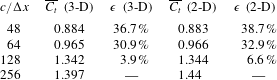
Grid convergence statistics for 3-D and 2-D simulations of a coupled motion case at  $Re=5300$,
 $A_{D}=1.5$ and
 $\unicode[STIX]{x1D703}_{bias}=0$. Here
 $\unicode[STIX]{x1D716}$ is error relative to
 $c/\unicode[STIX]{x0394}x=256$.

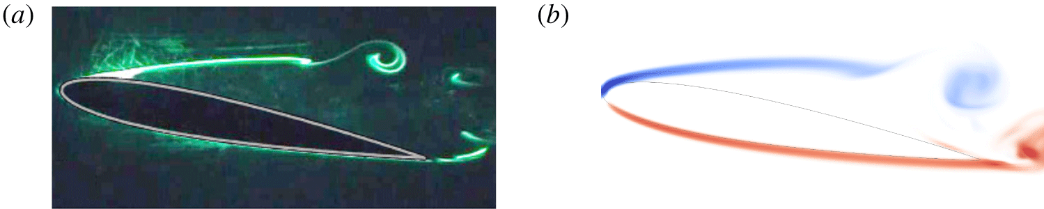
Accuracy comparison for instability starting location of a stationary NACA0012 foil at  $Re=5300$ and angle of attack 10°: (a) laser-induced fluorescence flow visualisation of Wang et al. (Reference Wang, Zhou, Alam and Yang2014), mean drag coefficient
 $C_{d}=0.14$, and (b) spanwise vorticity of 3-D simulation,
 $C_{d}=0.133$. The instability starts at the first vortex rollup.

The computational package used for this research is the boundary data immersion method (BDIM). Weymouth & Yue (Reference Weymouth and Yue2011) introduced BDIM using a robust and efficient Cartesian grid with implicit large-eddy simulation (iLES) solver. BDIM uses analytic meta-equations for an immersed body in multiphase flow with a smoothed interface domain using an integral kernel. BDIM has been validated, proved suitable for moving bodies and capable of resolving the flow at  $Re=10^{5}$ within 5 % error for thrust prediction (Maertens & Weymouth Reference Maertens and Weymouth2015).
For computational consistency between 2-D and 3-D simulations, the 3-D grids are the spanwise extrusion of 2-D grids and both simulations use the same iLES solver. Periodic boundary conditions are enforced along the spanwise direction of the foil and a span length of  $6c$ is used for 3-D simulation. The verification of grid convergence for 2-D and 3-D cases was carried out at
 $Re=5300$ to identify the appropriate grid required. Table 1 shows a comparison of the time-averaged thrust coefficient for different resolutions. It is seen that at a resolution of
 $c/\unicode[STIX]{x0394}x=128$, the force coefficient converges to within 7 % of the finer simulations (in both 2-D and 3-D cases). As a balance between the grid resolution and the number of simulations, a resolution of
 $c/\unicode[STIX]{x0394}x=128$ is deemed sufficient to capture the dynamics of the flow, and the parametric study in the following sections was carried out at this resolution but at a higher Reynolds number. A 3-D simulation for a stationary NACA0012 foil is compared with the experimental result of Wang et al. (Reference Wang, Zhou, Alam and Yang2014) in figure 2, showing an accurate instability location, and the drag coefficient is within 5 %.
3 Comparison between two- and three-dimensional simulations
The 2-D and 3-D simulations are further compared based on the vortex-structure evolution, mean force coefficients ( $\overline{C_{t}}$ and
 $\overline{C_{l}}$), phase-averaged spanwise component of vorticity and fluctuations of force-coefficient signals.
3.1 Overview and flow structures
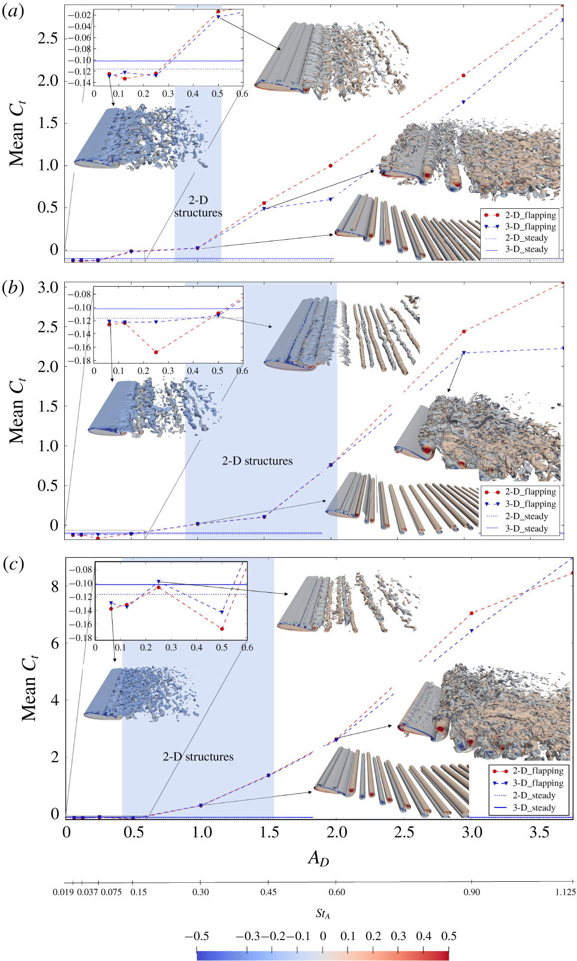
Figure 3 shows the variation of  $\overline{C_{t}}$ with
 $St_{A}$ for 2-D and 3-D simulations across three different kinematics (heave, pitch and coupled motions). The insets show isosurfaces of spanwise vorticity (
 $\unicode[STIX]{x1D714}_{z}$) for a few selected cases (linked with arrows in the various panels). Starting at the lowest
 $A_{D}$ (the lowest
 $St_{A}$), the flow structures appear to be 3-D with strong separation on the foil suction side similar to a stationary foil. The values of
 $\overline{C_{t}}$ for both 2-D and 3-D simulations appear to be very similar to the
 $\overline{C_{t}}$ of a stationary foil with a small discrepancy between 2-D and 3-D simulations.
Three-dimensional isosurfaces of  $\unicode[STIX]{x1D714}_{z}$ superimposed on mean thrust coefficient
 $\overline{C_{t}}$ versus trailing-edge amplitude
 $A_{D}$ graphs showing structure transitions at (a) heaving, (b) pitching and (c) coupled motions. Shaded areas locate 2-D structures and non-shaded for 3-D structures.

With a slight increase in amplitude, the flow structures appear to be more coherent and become more 2-D. The  $\overline{C_{t}}$ of 2-D and 3-D simulations now collapse onto the same value(s). These 2-D structures are found to persist until around
 $A_{D}=1$ or
 $St_{A}=0.3$ in all three types of motion. The beginning of 2-D flow structures is accompanied by propulsive wakes evolving into reverse Bénard–von Kármán in coupled motion or to asymmetric/deflected in heave and pitch. When
 $A_{D}$ increases even higher, the 3-D flow structures reappear, eliminating the uniform 2-D structures. They are followed by a substantial discrepancy in
 $\overline{C_{t}}$ between 2-D and 3-D simulations. The vortices appear to break down along the spanwise direction in the wake, and this breakdown starts to creep up to the trailing edge with increasing amplitude, which is consistent with the observations of Moriche et al. (Reference Moriche, Flores and García-Villalba2016). The flow structures at the trailing edge are more ‘chaotic’ along the spanwise direction, while the LEVs are relatively coherent along the span even at higher
 $A_{D}$.
The appearance of uniform 2-D structures in all three types of motion shows that 2-D simulations would indeed be sufficient over a certain range of Strouhal numbers, but the ranges are not the same for the three types of motion. The range is very limited for heaving motion, while the range is very similar for both pitching and coupled motions but the transition to 3-D is earlier for the coupled motion. The similarity between pitching and coupled motion is understandable, as the coupled motion is dominated by pitch motion in these current simulations. A heave-dominant coupled motion would lead to the breakdown of 2-D structures earlier and the range would be more similar to heaving-only motions.
3.2 Effect of spanwise domain size
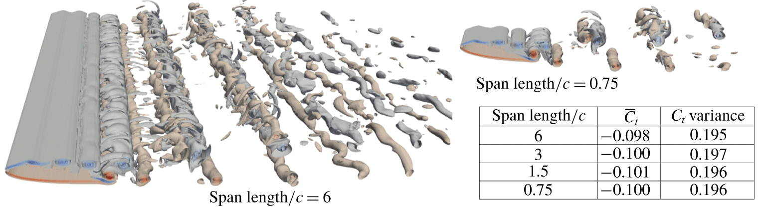
In order to isolate the effect of spanwise domain size of the 3-D simulations on the results observed above, a series of simulations with different spanwise lengths were carried out. All the simulations were confined at one kinematics: coupled motion at  $A_{D}=0.25$ where 3-D structures begin to reorganise into 2-D structures. Figure 4 shows that, even when the span is reduced at
 $0.75c$, the
 $\overline{C_{t}}$ and
 $C_{t}$ variances are almost constant and the 3-D structures remain significant. This signifies the importance of the three-dimensionality of the spanwise vortices. This also suggests that a small spanwise domain length might be sufficient to capture the 3-D effects provided the kinematics are in a certain range of amplitudes and frequencies.
Convergence of  $\overline{C_{t}}$ and
 $C_{t}$ variances with reduction in spanwise domain.

3.3 Statistics of thrust coefficient
Along with the appearance of uniform 2-D structures, the statistics of force coefficients ( $C_{t}$ and
 $C_{l}$), i.e. average, maximum, minimum and variance, are similar for both 2-D and 3-D simulations. At lower and higher
 $A_{D}$, when 3-D structures appear, the force coefficients in 2-D simulation exhibit very high levels of fluctuations. Similar force-coefficient fluctuations are shown for 2-D simulation by Taira & Colonius (Reference Taira and Colonius2009) for stationary flat plates at a higher angle of attack.
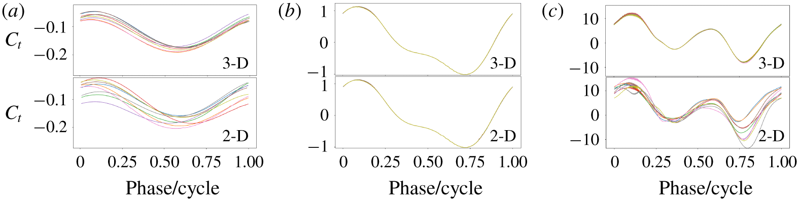
Figure 5 presents the comparison of  $C_{t}$ evolution for both 2-D and 3-D simulations for pitching motion. The tendencies of
 $C_{t}$ evolution for heaving and coupled motion are similar (not presented here for brevity). It can be seen that the 2-D simulations exhibit cycle-to-cycle variations at lower and higher
 $A_{D}$, while these variations are minimal for the intermediate amplitude. The cycle-to-cycle variations for the 3-D simulations are weaker and only apparent for the low-amplitude case. It was also found that both 2-D and 3-D simulations converged faster for the intermediate amplitude, since the variations in the flow and the forces are minimal.
Comparison of  $C_{t}$ between 2-D and 3-D simulations of pitching motion for 10 cycles at (a)
 $A_{D}=0.0625$, (b)
 $A_{D}=1$ and (c)
 $A_{D}=3.75$.

3.4 Spanwise vorticity
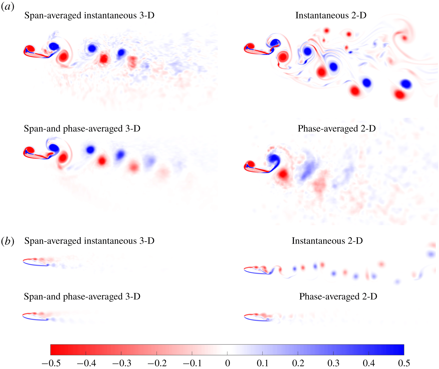
The instantaneous  $\unicode[STIX]{x1D714}_{z}$ and the phase-averaged
 $\unicode[STIX]{x1D714}_{z}$ for 2-D and 3-D simulations are compared in figure 6. For the 3-D simulations, the vorticity is first spanwise-averaged prior to comparing it with 2-D simulations. Presented are the cases where 3-D structures appear at the lowest and the highest
 $A_{D}$ in coupled motion. These are representative, and similar features are observed in other kinematics as well.
As seen in figure 6(a) for a flapping amplitude of  $A_{D}=3.75$, the instantaneous cases for 2-D and 3-D simulations differ mainly in the wakes. The wakes in 2-D simulation appear to be aperiodic and perhaps more chaotic. Meanwhile, the span-averaged vorticity in 3-D simulations appears ‘cleaner’ and more converged, making phase averaging easier. This is because, in 3-D simulations, the effect of spanwise averaging eliminates small perturbations in
 $\unicode[STIX]{x1D714}_{z}$ structure. However, in 2-D simulations, this is not possible. Any small variation is exacerbated since there is no smoothing process, and this leads to the appearance of a chaotic wake.
Instantaneous and phase-averaged  $\unicode[STIX]{x1D714}_{z}$ for coupled motion at (a)
 $A_{D}=3.75$ and (b)
 $A_{D}=0.0625$. The 3-D simulations have been span averaged prior to phase averaging. Supplementary movies are provided.

In phase-averaged coupled motion (similar to other kinematics), the LEVs appear to be slightly smaller for 2-D simulations compared to 3-D simulations due to ‘jitter’ in the position of these vortices over different cycles. On the other hand, both types of simulations preserve one vortex pair behind the trailing edge. In the ‘far’ wake, 2-D simulations are chaotic since the vortices are strong and their self-induced motions alter the trajectories of the wake. Moreover, there are no mechanisms that can reduce the strength of these vortices (other than viscosity) and therefore they remain strong for an extended length/time. For the 3-D simulations, the spanwise length provides a route for the transport of vorticity from the vortex core, thereby weakening the wakes downstream.
At the lowest  $A_{D}$ in figure 6(b), the difference between 2-D and 3-D simulations are not only in the wakes but also in the separation and recirculation areas. Similar to high
 $A_{D}$, the wakes for instantaneous 3-D simulation have the spanwise direction to transport/diffuse vorticity compared to 2-D simulations. Nonetheless, the wake widths of phase-averaged 2-D and 3-D simulations are similar. This perhaps explains why the difference in values of
 $\overline{C_{t}}$ in 2-D and 3-D simulations at lower
 $A_{D}$ is relatively small. At lower
 $A_{D}$, the LEVs in both 2-D and 3-D simulations look similar but the trailing-edge vortices (TEVs) are different due to recirculation and flow inside the separation region. The vortices in 2-D simulations at the separation region oscillate back and forth, while in 3-D simulations they are more stable (see supplementary movies available at https://doi.org/10.1017/jfm.2019.1078). This oscillation appears at a lower frequency than the shedding frequency, which explains the appearance of additional low-frequency energy content in 2-D simulation (see next section).
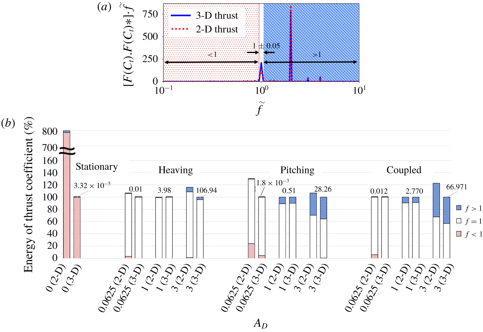
(a) Category division for  $C_{t}$ power spectra versus frequency (normalised to flapping frequency), and (b)
 $C_{t}$ power spectra integral or variance in percentage for three different
 $A_{D}$ values. Each 3-D bar is scaled as 100 % with its total variance on top, provided with the category divisions and accompanied by 2-D on its left scaled as a percentage corresponding to the 3-D.

3.5 Fourier analysis of force time histories
The power spectral density for the thrust coefficient time history is computed and plotted against frequencies normalised by the flapping frequency in figure 7(a). The peak frequency at  $\tilde{f}=1$ shows the flapping frequency. The ordinate is premultiplied by the frequency and presented in linear scale to ensure that equal areas under the curve represent equal ‘energy’. The term ‘energy’ here is used to represent the strength of the fluctuations in the signal. In fact, it should be noted that the total area under the curve is equal to the variance of the
 $C_{t}$ signal. Furthermore, the fluctuations can be categorised into three main regimes:
 $\tilde{f}<1$ (low frequency),
 $\tilde{f}=1$ (exactly at the flapping frequency) and
 $\tilde{f}>1$ (high frequency). The integrals of the areas under the curves within these regimes provide the contributions from each of these regimes to the overall fluctuations.
Figure 7(b) shows a bar chart that compares the energy in force fluctuations from 2-D simulations to their 3-D counterparts. The total variance from the 3-D simulations is taken as the reference to calculate percentages, and this numerical value is indicated at the top of the bars. Consequently, the bars for the 2-D simulations are sometimes higher than 100 % since the variance in 2-D is higher than in 3-D simulations. The contributions of three regimes to these fluctuations are shown in three colours as marked in figure 7(a). Different bars are shown for different kinematics and flapping amplitudes. Two bars on the left are also shown for the stationary foil where the total energy of 2-D simulation is eight times higher than the 3-D value. However, the absolute values of these fluctuations are orders of magnitude smaller than the flapping motions as seen from the numerical value on the top of the bars.
It is clear from figure 7 that the appearance of coherent 2-D structures is accompanied by a very similar distribution of fluctuations in the three different regimes in 2-D and 3-D simulations. Meanwhile, the appearance of 3-D structures (spanwise variations) is accompanied by the discrepancy of force fluctuation variance between 2-D and 3-D simulations, where 2-D simulation tends to exaggerate the levels of force fluctuations. Pitching has the lowest total energy among the three types of motion due to the nature of its kinematics, while pure heaving motion produces the largest levels of fluctuations. Meanwhile, coupled motion energy is slightly lower than heaving because of the 90° phase lag between the pitching and heaving parts of the motion.
The vortex shedding frequency of a stationary foil also appears in the flapping foil (as a low frequency) and can be seen to contribute to force fluctuations for low values of  $A_{D}$. However, 2-D simulations exhibit other additional low frequencies, which stem from cycle-to-cycle variations as discussed in the previous section. As
 $A_{D}$ increases, the energy from kinematics far exceeds the energy from vortex shedding. This explains the transition from 3-D to 2-D uniform structures. The energy from kinematics arranges the flow structures into uniform reattaching separation zone so that the vortices move consistently from the leading edge until detachment at the trailing edge, leading to more organised downstream wakes. At higher values of
 $A_{D}$, higher harmonic frequencies start to appear and these make a contribution to the force fluctuations. The contributions from these higher frequencies are significantly higher in 2-D simulations compared to 3-D simulations since there are additional higher frequencies due to the appearance/movement of chaotic vortices as seen in figures 5 and 6.
It is seen that coupled and pitching motions have large contributions (over 20 %) from  $\tilde{f}>1$ at high values of
 $A_{D}$. The relative contributions are small for heave motions; however, since the absolute values of fluctuations in heave motions are much higher than other kinematics (as seen by the numerical value at the top), the absolute value from
 $\tilde{f}>1$ is very comparable across different kinematics. This suggests that there could be a universal mechanism that leads to higher-frequency force fluctuations regardless of kinematics. This mechanism could be related to the breakdown of the LEVs along the spanwise direction. This is further explored below.
3.6 Breakdown of leading-edge vortices
The transition from 2-D back to 3-D with increasing  $A_{D}$ is expected to be due to spanwise instability that leads to the breakdown of the vortices. As they grow in strength, vortices burst and form non-uniform small structures along the span. This breakdown appears to be at different values of
 $A_{D}$ for different kinematics. This can be examined by calculating the circulation of the LEV for different values of
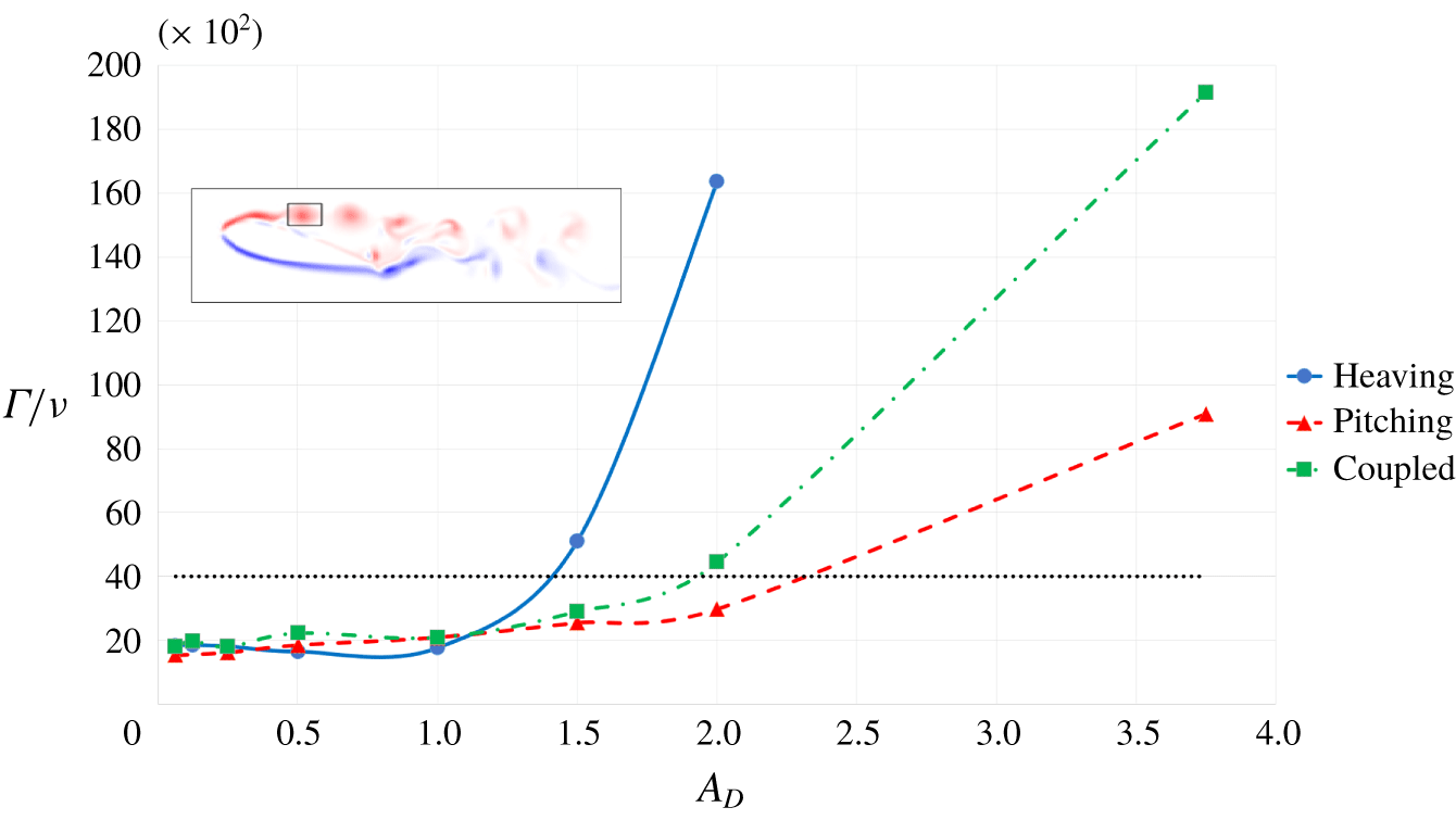
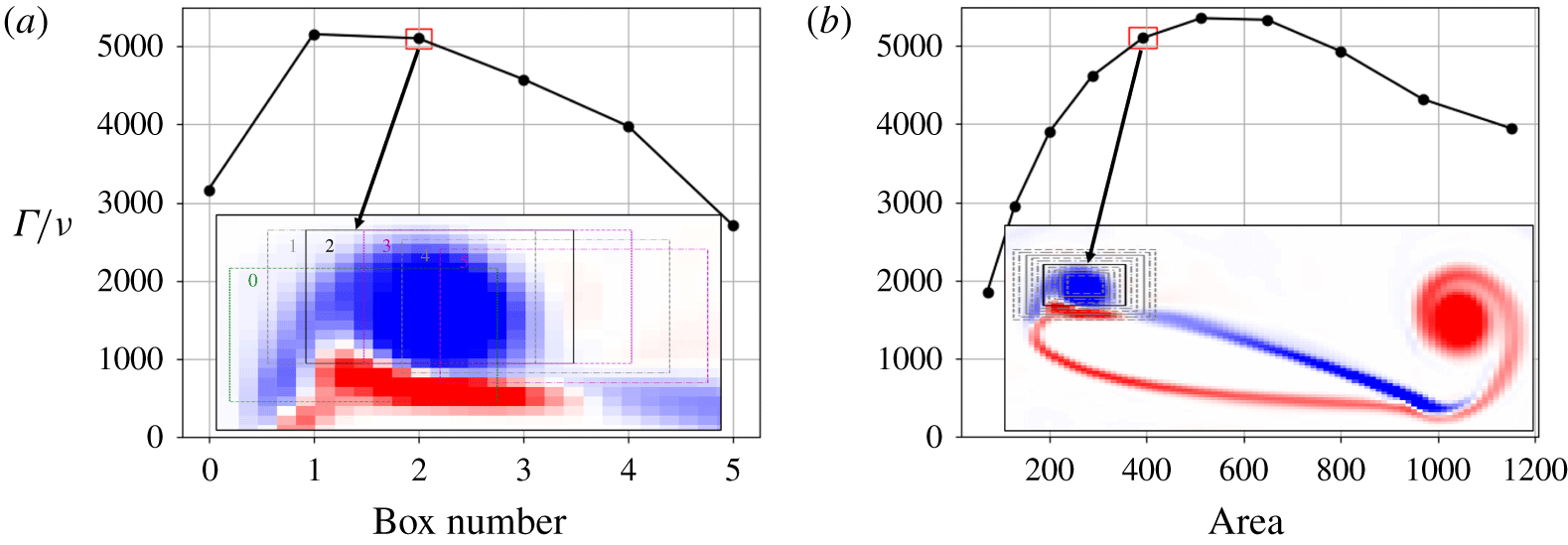
 $A_{D}$ and different kinematics. Figure 8 shows the variation in the circulation of LEVs, now represented as a Reynolds number (with
 $Re=\unicode[STIX]{x1D6E4}/\unicode[STIX]{x1D708}$). This circulation is calculated as the integral of vorticity over a box as shown in the inset in figure 8. This box was chosen at a given phase where a vortex is just shed from the leading-edge separation bubble. Since the frequency of flapping is the same for all simulations, the location and size of this box did not have to change across the different kinematics. The sensitivities for box sizes and locations are provided in figure 9, showing that
 $\unicode[STIX]{x1D6E4}$ is robustly estimated as long as the integration region encloses the LEV pinch-off location. Finally, a comparison of the circulation between 2-D and 3-D simulations did not reveal any noticeable difference before the vortices start to break down. This is because we are examining the ‘first’ vortex that is shed, which are very similar regardless of the case.
Figure 9 indicates that Reynolds numbers (or circulation) of the LEVs appear to grow exponentially with increasing  $A_{D}$. The rate of increase is different for different kinematics. Heaving motion leads to the fastest growth among the three types of motion resulting in the shortest range of Strouhal numbers with 2-D structures. In comparison, pitching and coupled motions have a more gradual growth, leading to wider ranges for the presence of 2-D structures. It should be noted that the coupled motion is dominated by pitching and therefore resembles the pitching kinematics.
The horizontal dotted black line in figure 8 indicates the circulation of the LEVs where uniform 2-D structures transition to 3-D structures. The cases where the circulations of LEVs are higher than this value show vortex breakdown and smaller-scale structures accompanied by force fluctuations in higher frequencies. This is universally true regardless of the kinematics. This circulation or Reynolds number of LEVs,  $\unicode[STIX]{x1D6E4}/\unicode[STIX]{x1D708}\approx 4000$, is the critical Reynolds number where the balance between vortex strength (induced by the kinematics) and viscous diffusion is lost leading to vortex breakdown. This critical Reynolds number is akin to the Reynolds number of a cylinder where there is a spanwise breakdown of vortices. However, for that case, the Reynolds number based on the cylinder diameter is much smaller than 4000. Regardless, the mechanism for the transition from 2-D to 3-D type flow structures appears to be similar.
Evolution of LEV circulation over kinematic viscosity along the increase of  $A_{D}$. The flow above the dotted black line shows 3-D structures.

Sensitivity analysis for heaving at  $A_{D}=1.5$: (a) box locations and (b) box sizes. The highlighted box size and location were chosen for the study and the results are shown in figure 8.

4 Conclusion
This work demonstrates that spanwise-uniform 2-D structures are discovered at intermediate  $St_{A}$ of a flapping foil, while strong 3-D structures are found at higher and lower
 $St_{A}$. These 3-D structures are produced over the span without being initiated by the tip effect. In the intermediate
 $St_{A}$ region with spanwise-uniform (2-D) structures, all statistics of force coefficients (lift and drag), such as mean, maximum and variance, are similar between 2-D and 3-D simulations. These 2-D structures are found at
 $St_{A}\approx 0.3$ in heaving motion,
 $St_{A}\approx 0.3{-}0.6$ in pitching and
 $St_{A}\approx 0.15{-}0.45$ in coupled motion. Critically, the coupled motion gives a sufficient range for 2-D structures to cover the optimal-efficiency
 $St_{A}$ region for swimming animals mentioned by Triantafyllou et al. (Reference Triantafyllou, Triantafyllou and GrosenBaugh1993), proving that 2-D simulations are valid in this region.
In the regions where 3-D vortex structures appear at higher and lower  $St_{A}$, we discover a discrepancy of mean force coefficients between 2-D and 3-D simulations and overprediction in 2-D simulation variances. The appearance of 3-D structures at lower
 $St_{A}$ is accompanied by more stable LEVs and discrepancies in the separation and recirculation areas. Meanwhile, the flow field of 2-D simulations at higher
 $St_{A}$ indicates non-dissipative vortices causing high force fluctuations and disturbance in the wake trajectories, LEVs and TEVs.
By analysing the variance of thrust-coefficient signals, we conclude that the transition from a3-D to 2-D vortex wake at intermediate  $St_{A}$ is due to the kinematics overwhelming the stationary foil’s 3-D drag wake. This is supported by the fact that the transition occurs at the same amplitude as the occurrence of reverse Bénard–von Kármán propulsive wakes. Meanwhile, the 2-D to 3-D transition from intermediate to higher
 $St_{A}$ is due to high-energy LEVs overpowering the damping effect of viscosity causing the LEVs to break down at
 $\unicode[STIX]{x1D6E4}/\unicode[STIX]{x1D708}\approx 4000$.
The application of strip theory may still be valid but only in the range of  $St_{A}$ where the flow structures are uniformly 2-D. Outside of this, the validity is questionable, signifying that the strip theory should not be applied at high
 $St_{A}$ or low
 $St_{A}$. The 2-D structure window is found to be relatively wider in pitch-dominating motion. For manoeuvring and taking off flying, where heaving motion is significant and normally at higher
 $St_{A}$, 3-D simulations are necessary regardless of the effect of tip vortices. In the future, this research will be continued using 3-D shape (including tip effect) and 3-D motion (rolling and twisting motions) to comprehensively study the application of strip theory to finite flapping foils.
Acknowledgements
We would like to thank the Indonesia Endowment Fund for Education (LPDP), the IRIDIS High Performance Computing Facility with its associated support services at the University of Southampton, the Office of Naval Research Global Award N62909-18-1-2091 and Dr K. Hendrickson at MIT for the completion of this work.
Declaration of interests
The authors report no conflict of interest.
Supplementary movies
Supplementary movies are available at https://doi.org/10.1017/jfm.2019.1078.