Introduction
Millimeter-wave radar systems are indispensable to the advanced driving assistance systems (ADAS) sensor suite. Radars can detect targets in adverse weather conditions, where cameras and LiDAR are often rendered ineffective due to limited visibility. This paper analyzes radars operating at 77–81 GHz. An earlier version of it was presented at the 19th Conference of Antennas and Propagation (EuCAP 2025) and published in its proceedings [Reference Gupta, Varga, Hein and Dallmann1].
Precipitation can significantly impact automotive radar performance due to scattering, absorption, diffraction, and depolarization effects. This leads to signal attenuation and a reduced dynamic range, which can cause ghost targets. Therefore, understanding how precipitation scattering affects radars and developing suitable models allows us to evaluate the limitations of these radars. However, physical road tests in varying weather conditions are unpredictable and not reproducible. Hence, virtual testing to simulate real-world scenarios is a more practical solution.
Radar target emulators, together with software, hardware, and vehicle-in-the-loop (SiL/HiL/ViL) test setups, provide controlled and repeatable environments for evaluating radar sensors and perception algorithms [Reference Buddappagari, Asghar, Baumgärtner, Graf, Kreutz, Löffler, Nagel, Reichmann, Stephan and Hein2–Reference Sievers, Seiger, Peperhowe, Krumm, Graf and Hanselmann5]. To realistically include rain effects in such frameworks, precipitation must first be understood and modeled as an isolated physical phenomenon. This avoids confounding influences such as wind or multipath propagation, which can be better addressed in dedicated future studies. Treating precipitation effect independently allows it to be flexibly overlaid onto existing radar scenarios. Accordingly, this paper models rain back-scatter clutter using an empirical approach suitable for virtual radar simulations.
Related work
Mie theory
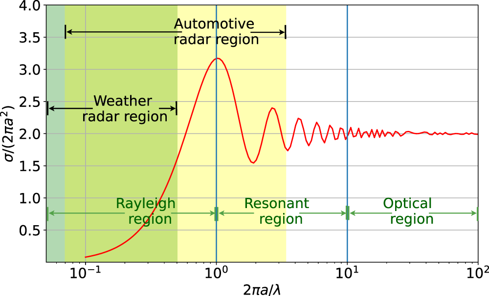
Mie scattering theory describes the dependence of the radar cross-section (RCS)  $\sigma$ of a spherical particle on the ratio of its size to the radar wavelength
 $\lambda$ [Reference Skolnik6]. As depicted in Figure 1, it can be classified into three scattering regions. In the Rayleigh region, the size of the sphere is much smaller than the wavelength. In the resonant region, the size of the sphere is in the order of the wavelength, and in the optical region, the size of the sphere is much larger than the wavelength. Precipitation particles, such as raindrops, range in size from approximately 0.1 to 8 mm [Reference Hobbs and Rangno7]; the size parameter can be calculated for automotive radars. Based on their frequency band and the size of rain droplets, they cover two scattering regions. This makes it unsuitable to apply Rayleigh, resonant, or optical approximations individually.
Perfect conductor sphere scattering (radius  $a$).

Figure 1 Long description
The x axis label is, 2 pi a over lambda. The x axis shows 10 superscript minus 1, 10 superscript 0, 10 superscript 1 and 10 superscript 2. The y axis label is, sigma over 2 pi a superscript 2. The y axis ranges from 0.0 to 4.0. A single line is plotted. It starts near x equals 10 superscript minus 1 at about y equals 0.1. It rises to a peak near x equals 10 superscript 0 at about y equals 3.2. It then drops to about y equals 1.6 near x around 2. It rises again to about y equals 2.4 near x around 3, then drops to about y equals 1.8 near x around 4. From about x around 4 to x around 10 superscript 2, the line shows repeated small oscillations around y equals 2.0. Text labels inside the plot read, Weather radar region, Automotive radar region, Rayleigh region, Resonant region and Optical region.
Automotive radars
Current papers on precipitation in automotive radar technology focus on attenuation occurring due to forward scattering. As referred from the ITU-R P.838 model [8, Reference Zhao, Zhang and Wu9],
 \begin{equation}
A = aR^b
\end{equation}
expresses a power-law relationship, specifying rain attenuation. Here,  $A$ is attenuation in dB/km,
 $R$ is rain rate in mm/h, and coefficients
 $a$ and
 $b$ depend on transmission frequency and atmospheric temperature. These coefficients have been derived through logarithmic regression and Mie scattering calculation. However, as mentioned in [Reference Olsen, Rogers and Hodge10], this relation is most accurate for the X- to K- band frequency range. Also, attenuation for automotive radar operating at 77 GHz for rain rates up to 100 mm/h over their maximum range of 350 m is approximately 11 dB [Reference Gourova, Krasnov and Yarovoy11]. Despite the extreme rain rates at the maximum range, the attenuation remains relatively modest and does not significantly affect the operational capability of the radar.
Moreover, back-scattering caused by precipitation incites an increase in clutter level in the received signal, which reduces dynamic range and can lead to ghost targets. There have been some recent developments in the investigation of rain clutter for automotive radar. [Reference Gourova, Krasnov and Yarovoy11, Reference Jang, Jung, Soo Chong, Sung and Lim12] discuss the effect of rain attenuation on target detection. Additionally, in [Reference Richard, Kammerer and Wallace13], experiments were conducted with 9.375, 35, 70, and 95 GHz radars to measure rain back-scattering and develop its macroscopic power-law relationship with rainfall rate. The study utilized outdoor measurements and primarily served to verify fundamental Mie scattering physics. Also, the rain clutter modeling for E-band radars remains largely unexplored. Therefore, this paper aims to comprehensively investigate and develop an empirical statistical model of back-scattering from precipitation clutter for 77–81 GHz radars.
Back-scattering can be characterized by the RCS, which is the power density reflected by a target in relation to the power density radiated by the radar’s transmitter antenna in the target vicinity. For volumetric targets, such as rain droplets, RCS in  $\text{m}^2$ can be further expressed as [Reference Skolnik6]
 \begin{equation}
\sigma = \eta V
\end{equation}
Here,  $\eta$ is the clutter reflectivity factor in
 $\text{m}^{-1}$ and
 $V$ is the volume illuminated by the radar within a particular range in
 $\text{m}^3$. Rain reflectivity is a function of raindrop size distribution and back-scattering from each raindrop. This paper attempts to model
 $\eta$ for different rain rates based on measured data. The measurement setup is explained in detail in the third section, followed by the analysis of the measured data in the fourth section. Results are discussed in the fifth section and summarized in the sixth section.
Measurement setup
Measurements were conducted at the CARISSMA Research Center in Ingolstadt, Germany [14], which is a controlled indoor facility. It has an asphalt track with road markings and a concrete divider covered by microwave absorbers on one side, as shown in Figure 2. A 50 m long irrigation system is installed above the track, producing adjustable rain intensity and drop size distribution. Rain for the measurements was generated at rain rates of 16, 32, 66, and 98 mm/h, which all follow the corresponding Marshall–Palmer rain distribution and thus resemble realistic rainfall [Reference Marshall and Palmer15].
Measurement setup at CARISSMA.

Figure 2 Long description
Radar measurement setup with a rain area and a triple reflector on an asphalt track. The radar is positioned on the left side, marked with dimensions of 3.945 meters in width and 5.172 meters in height. The rain area is indicated in the center, with arrows showing different measurement paths labeled R superscript 11 subscript 11, R superscript 15 subscript 11, R superscript 20 subscript Baseline and R superscript 18 subscript 11. These paths are represented by arrows of different colors: red, blue, green and purple, respectively. The arrows are positioned at heights of 2.5 meters, 0 meters and minus 2.5 meters, indicating the vertical alignment of the measurements. The triple reflector is located 30 meters from the radar, along the asphalt track, which extends from 0 to 50 meters. Below the track, a concrete divider with absorbers is shown, followed by a wall at the bottom. The x-axis represents the horizontal distance, while the y-axis indicates the vertical position of the measurement paths.
The measurements were conducted for two setups, the first one with a triple reflector (TR) and the second one without TR and therefore agreeing with a background (BG) measurement. The TR was measured at 20, 30, 40, and 50 m and supplemented by a corresponding BG measurement for each given rain rate except 98 mm/h. For 98 mm/h, only measurements at 30 m were taken. Data was recorded with the Continental 77 GHz radar sensor ARS430 [16]. The radar sensor provides a detection list with RCS in dBsm, azimuth angles in rad, time stamps in ms (Coordinated Universal Time) and range bins in m.
Methodology
This paper analyzes measurements for TR and BG setups at distances of 20, 30, 40, and 50 m at rain rates of 16, 32, and 66 mm/h, as well as 30 m at a 98 mm/h rain rate. In total, 26 measurements were analyzed, each referred to as a scenario in the following.
Based on the azimuth and elevation half-power beamwidth of the radar antenna, the elliptical frustum volume for each range cell is calculated to obtain the rain reflectivity,  $\eta$:
 \begin{equation}
V = \frac{\pi}{3} \tan\left(\frac{\phi_\Delta}{2}\right) \tan\left(\frac{\theta_\Delta}{2}\right) \left(\frac{r_\Delta^3}{4} + 3 r_\Delta r^2\right)
\end{equation}
Here,  $V$ is the volume in
 $\text{m}^3$,
 $\phi_\Delta$ is the half-power beamwidth in the azimuth (horizontal) direction in rad,
 $\theta_\Delta$ is the half-power beamwidth in the elevation (vertical) direction in rad,
 $r_\Delta$ is the range resolution in m, and
 $r$ is the measured range bin of the target region in m.
Data outside the defined area under test ( $R_{y_{min}}^{y_{max}}$), restricted to
 $x \in [-2.5~\text{m},~2.5~\text{m}]$ and
 $y \in [y_{\min},~y_{\max}]$, were discarded to avoid reflections from the ceiling, walls, and a concrete divider (see Figure 2). The reference model is based on the
 $y$-axis observation range of
 $y \in [10~\text{m},~20~\text{m}]$, hereafter referred to as
 $R_{10}^{20}$. In addition, three alternative
 $R_{y_{min}}^{y_{max}}$ ranges were analyzed:
 $R_{10}^{11}$ with
 $y \in [10~\text{m},~11~\text{m}]$,
 $R_{10}^{15}$ with
 $y \in [10~\text{m},~15~\text{m}]$, and
 $R_{10}^{30}$ with
 $y \in [10~\text{m},~30~\text{m}]$.
The rain back-scattering clutter model is primarily based on  $R_{10}^{20}$, as it provides a sufficient detection density along its whole range. Since the number of raindrop detections by automotive radar decreases with increasing distance from the sensor,
 $R_{10}^{20}$ serves as a suitable reference. Nevertheless, to investigate the influence of spatial configuration, additional
 $R_{y_{min}}^{y_{max}}$ ranges were also analyzed.
Adaptive binning
A histogram was created for each scenario to model the data empirically. Table 1 presents the sample statistics. The distributions are strongly skewed (skewness 5.3–8.8, overall mean  $ \gt 10$), indicating heavy tails across all rain rates. The outliers comprise only around 1–2% (with an overall mean
 $ \lt 2\%$) of the data, yet they strongly affect the statistical histograms. Such characteristics show that fixed-width binning is ineffective. The strong skewness and sparse but extreme outliers force most low values into a very few bins, thereby flattening the higher range. Therefore, adaptive binning is required to preserve detail in dense regions while still accounting for outliers.
Sample statistics of different scenarios with the overall mean computed over the full data set

In earlier work [Reference Gupta, Varga, Hein and Dallmann1], this issue was addressed by removing  $0.1\%$ outliers prior to applying fixed-width binning. In contrast, the present work employs a robust adaptive binning strategy, which mitigates the impact of outliers more effectively and eliminates the need for outlier filtering. The binning approach follows a hierarchical decision process in which only one binning rule is ultimately applied, depending on the statistical characteristics of the data.
Freedman–Diaconis rule
As per Freedman–Diaconis (FD), the interquartile range (IQR) is a pragmatic measure of spread, where
 \begin{equation}
\text{Bin width} = 2\,\frac{\mathrm{IQR}}{n^{1/3}}
\end{equation}
Freedman and Diaconis introduced it in [Reference Freedman and Diaconis17]. Here, IQR refers to the data range between the first and third quartiles (Q1 and Q3). If this produces at least  $80\%$ of the desired number of bins (i.e., 500), it complies with the structure of the dense region by IQR resistance to outliers and yields enough resolution, so no further adjustment is needed and the algorithm terminates.
Log adaptive rule
If the FD IQR 25–75 rule produces substantially fewer bins than required, the absolute skewness of the data is evaluated. When the skewness exceeds a threshold of 3, and all values are positive, logarithmic binning is applied. The bins are spaced uniformly in the logarithmic domain and then mapped back to the linear scale. Logarithmic binning is well-suited for long-tailed or power-law distributions [Reference Clauset, Shalizi and Newman18], as it preserves resolution in dense regions while compressing the tail.
Modified FD rule
If the skewness does not exceed the threshold, a fallback method based on a modified FD rule is used. This method computes the bin widths from the data range between the 15th and 85th percentiles, thereby ignoring the most extreme  $15\%$ of values on each tail. The resulting bin widths are then applied to the full data range.
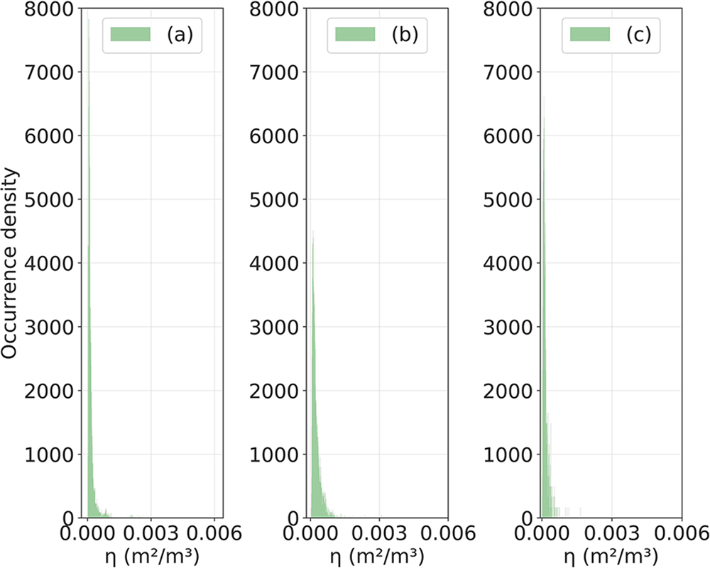
Figure 3 illustrates example histograms of the different datasets utilizing the different binning methods, showing  $\eta$ on the
 $x$-axis and the density of occurrence per bin on the
 $y$-axis. Depending on the data characteristics, a different adaptive binning rule is selected, and one representative example of each case is shown. To assess the uniformity of the data distribution across histogram bins, the Shannon entropy is computed as
Histograms with adaptive binning methods: (a) rain rate: 16 mm/h, scenario: TR 40 m, binning: FD IQR 25–75, (b) rain rate: 32 mm/h, scenario: TR 30 m, binning: log adaptive, and (c) rain rate: 16 mm/h, scenario: BG, binning: modified FD IQR 15-85.

 \begin{equation}
H = -\sum_i p_i \log p_i ,
\end{equation}
Here,  $p_i$ denotes the empirical bin probabilities [Reference Cover and Thomas19]. The entropy is normalized to
 $[0,1]$, with higher values indicating more uniform bin occupancy. Fixed-width binning yields an average entropy of
 $0.564$. Among the individual adaptive rules, the FD rule based on the
 $25$–
 $75$ IQR results in
 $0.557$, log-adaptive binning yields
 $0.564$, and the modified FD rule using the
 $15$–
 $85$ IQR achieves the highest average entropy of
 $0.663$. The proposed adaptive binning approach, which selects between these methods based on data characteristics, attains an average entropy of
 $0.592$ and outperforms individual strategies in certain cases, indicating improved robustness across datasets.
The distinct shape of the distribution, with a steep rise followed by a heavily skewed tail, necessitates an investigation to reproduce this behavior most effectively. The objective is to identify a model that optimally fits the data. To this end, the datasets were fitted with 119 probability distributions available in the SciPy statistics library [Reference Virtanen, Gommers, Burovski, Oliphant, Weckesser, Cournapeau, Peterson, Reddy, Haberland and Wilson20]. To achieve this, hyper parameters were calculated based on the data set properties and used in an exhaustive grid search to identify a list of local minima. This list was then used to initialize the Levenberg-Marquardt optimization algorithm [Reference Gavin21] to obtain optimized parameters for all the probability distribution fittings.
Probability distribution functions
The key probability distributions with the most relevance are given together with a description and their probability density function (pdf) below [Reference Papoulis and Pillai22].
Rayleigh distribution
The Rayleigh distribution is commonly used to model the magnitude of a vector with normally distributed components and for stochastic modeling of RCS in Swerling models III and IV [Reference Blair and Brandt-Pearce23]. Its pdf is given by
 \begin{equation}
f(x; \varsigma) = \frac{x}{\varsigma^2} e^{-\frac{x^2}{2\varsigma^2}}, \quad x \geq 0
\end{equation}
Here  $ \varsigma \gt 0 $ is the scale parameter.
Exponential distribution
The exponential distribution is commonly used to model the time until the next event occurs, under the assumption that events take place at a constant average rate. It is also applied in stochastic modeling of RCS within the Swerling I and II models [Reference Blair and Brandt-Pearce23, Reference Richards24]. Its pdf is given by
 \begin{equation}
f(x; \lambda) = \lambda e^{-\lambda x}, \quad x \geq 0 ,
\end{equation}
where  $ \lambda \gt 0 $ is the rate parameter.
Furthermore, if the Rayleigh distribution is defined as  $R \sim \mathrm{Rayleigh}(\sigma) $, then its square
 $E = R^2$ follows an exponential distribution. This implies that when the amplitude
 $ R $ of the received radar signal is Rayleigh distributed, the corresponding power, which is proportional to
 $ R^2 $, follows an exponential distribution.
Rician distribution
The Rician distribution describes the magnitude of a circularly symmetric normal random variable, often used in signal processing to describe fading channels. It generalizes the Rayleigh distribution by introducing a non-centrality parameter [Reference Van Valkenburg25]. Its pdf is given by:
 \begin{equation}
f(x; \nu, \varsigma) = \frac{x}{\varsigma^2} e^{-\frac{(x^2 + \nu^2)}{2\varsigma^2}} \text{I}_0\left( \frac{x\nu}{\varsigma^2} \right), \quad x \geq 0
\end{equation}
Here  $ \nu $ is the non-centrality parameter,
 $ \varsigma $ is the scale parameter, and
 $\text{I}_0$ is the modified Bessel function of the first kind.
Weibull distribution
The Weibull distribution is a versatile distribution employed in reliability engineering, life data analysis, and modeling failure times. It generalizes the exponential distribution by introducing a shape parameter. Its pdf is given by
 \begin{equation}
f(x; \lambda, k) = \frac{k}{\lambda} \left( \frac{x}{\lambda} \right)^{k-1} e^{-(\frac{x}{\lambda})^k}, \quad x \geq 0
\end{equation}
Here  $ \lambda \gt 0 $ is the scale and
 $ k \gt 0 $ is the shape parameter.
Gamma distribution
The gamma distribution generalizes the exponential distribution and is commonly required to model waiting times or the sum of independent exponentially distributed random variables. Its pdf is given by
 \begin{equation}
f(x; \alpha, \beta) = \frac{\beta^\alpha x^{\alpha-1} e^{-\beta x}}{\Gamma(\alpha)}, \quad x \geq 0
\end{equation}
Here  $ \alpha \gt 0 $ is the shape parameter,
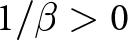 $ 1/\beta \gt 0 $ is the scale parameter, and
 $ \Gamma(\alpha) $ is the gamma function. The gamma distribution can also be defined in terms of the shape parameter (
 $\alpha$) and the rate parameter (
 $\beta$), where the rate is the reciprocal of the scale parameter.
Inverse-Weibull (IW) distribution
The inverse-Weibull (IW) distribution is obtained by taking the reciprocal of a Weibull-distributed variable. If a random variable  $W$ follows a Weibull distribution with shape parameter
 $k$ and scale parameter
 $\lambda$, given by
 $ W \sim \mathrm{Weibull}(k, \lambda)$, then the reciprocal
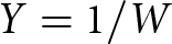 $Y = 1/W$ follows an IW distribution characterized by the same shape
 $k$ and scale
 $\lambda$. Its pdf is [Reference Babacan26, Reference Hassan and Nassr27].
 \begin{equation}
f(x; k, \lambda) = \frac{k}{\lambda^k} \, x^{-\,k-1} e^{-(\frac{\lambda}{x})^k},
\quad x \gt 0
\end{equation}
Here,  $k \gt 0$ controls the shape of the distribution, and
 $\lambda \gt 0$ is the scale parameter. Moreover, it can be noted that a random variable
 $W$ following the Weibull distribution can also be considered a linearization of its reciprocal
 $Y=1/W$, in the sense that the reciprocal can be described by the first-order term of a Taylor expansion.
Inverse-gamma (IG) distribution
The inverse-gamma (IG) distribution is a probability distribution of a variable’s reciprocal that follows a gamma distribution. If a random variable  $X$ follows a gamma distribution with shape parameter
 $\alpha$ and rate parameter
 $\beta$ (so that its scale is
 $1/\beta$), denoted
 $X \sim \mathrm{Gamma}(\alpha,\beta)$, then the reciprocal variable
 $Y = 1/X$, follows an IG distribution with the same shape parameter
 $\alpha$ and scale parameter
 $\beta$. It constitutes a two-parameter ensemble characterized by the shape parameter
 $\alpha$ and the scale parameter
 $\beta$ [Reference Cook28].
 \begin{equation}
f(x; \alpha, \beta) = \frac{\beta^\alpha}{\Gamma(\alpha)} x^{-(\alpha+1)} e^{(-\frac{\beta}{x})}, \quad x \geq 0
\end{equation}
Here,  $\alpha$ is the same shape parameter as in the gamma distribution and
 $\beta$ is the scale parameter, which is numerically equivalent to scale parameter
 $1/\beta$ of the gamma distribution. Similarly to what was explained in the previous subsection, it can be noted that a random variable
 $X$ following the gamma distribution can also be considered a linearization of its reciprocal
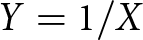 $Y=1/X$, following an IG distribution.
Others
Apart from the previously considered PDFs, the log-normal, inverse-Gaussian, Landau, and Gibrat distributions all produced lower overall error cost than the gamma distribution, which had been identified as the best fit in earlier analyses. However, none of them outperformed the IG or IW distributions, so they are not considered further here.
Results and discussion
Evaluation methodology
After optimization and parameter estimation, the residual sum of squares (RSS) for each given distribution was calculated for each scenario by
 \begin{equation}
\textit{RSS}_n = \sum_i ( m_n(\eta_i) - f_n(\eta_i))^2
\end{equation}
Here,  $m_n(\eta_i)$ is the occurrence density and
 $f_n(\eta_i)$ is the estimated pdf at
 $\eta_i$ for each measurement
 $n$. The RSS quantifies the deviation between the fitted model and the observed data, with lower values indicating a closer agreement. Consequently, RSS provides a direct measure of the goodness of fit and enables the identification of the most suitable distribution for modeling the precipitation clutter statistics. For every tested distribution, the mean of
 $\textit{RSS}_n$ for all measurements was calculated (
 $\overline{RSS}$). The standard error mean (SEM) is given by
 \begin{equation}
\textit{SEM} = \frac{\varsigma}{\sqrt{N}}
\end{equation}
Here,  $\varsigma$ is the standard deviation of
 $\textit{RSS}_n$, and
 $N$ is the number of measurements, in this case 26.
Model validation
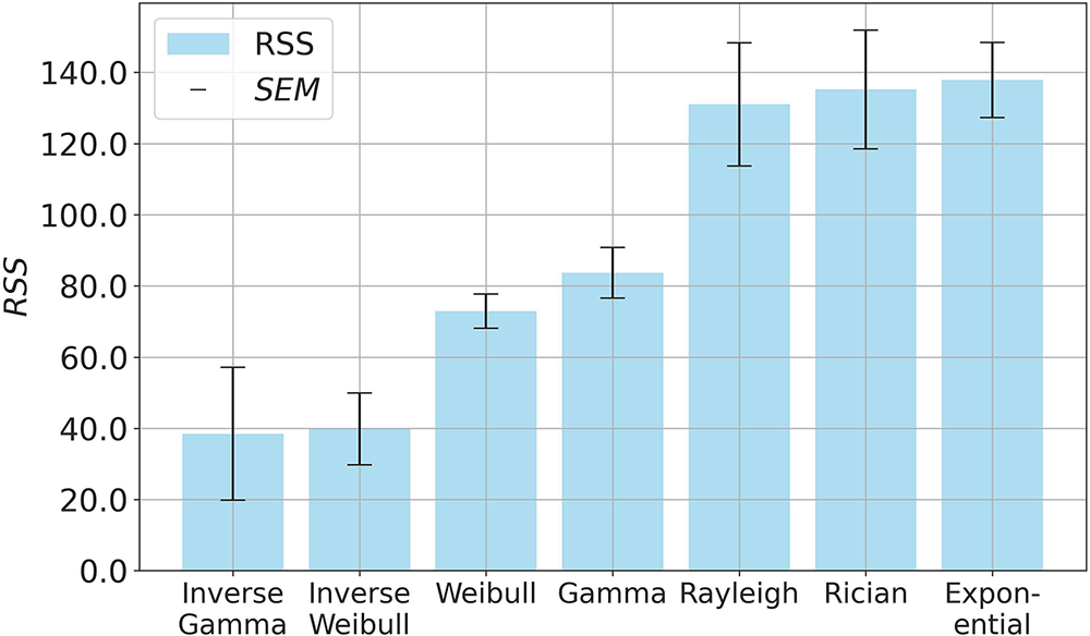
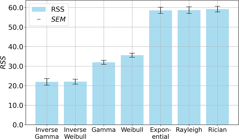
Since the statistically best-fitting model across all evaluated scenarios is the IG distribution, as shown in Figure 4, a Monte Carlo verification was conducted to validate the proposed methodology. IG distributed datasets were generated, and the complete analysis pipeline, including adaptive binning and probability density fitting, was applied. This procedure was repeated for 50 independent realizations. The results, compared to the main considered PDFs, are shown in Figure 5. An overlap with the IW distribution is also observed, which is expected due to the similar heavy-tailed and positively skewed characteristics shared by both distributions. Nevertheless, the IG distribution was identified as the best-fitting model, demonstrating that the proposed binning and fitting framework reliably recovers the underlying distribution and does not introduce systematic bias.
Error across distributions for  $R_{10}^{20}$.

Validation of the proposed framework.

To further quantify the goodness of fit, the Kolmogorov–Smirnov (KS) distance [Reference Stephens29] between the empirical distribution and the fitted IG model was evaluated and found to be approximately 0.015. The KS distance measures the maximum deviation between the empirical and model cumulative distribution functions, with smaller values indicating closer agreement between the two. A KS distance this low is generally indicative of a good fit, suggesting that the fitted IG model closely captures the empirical distribution.
Characteristics of the baseline range
As mentioned in the fourth section, the key modeling is based on  $R_{10}^{20}$, for which a comparison of RSS and SEM for all considered distributions is provided in Figure 4. The bars indicate the RSS for each distribution, while the whiskers represent the SEM.
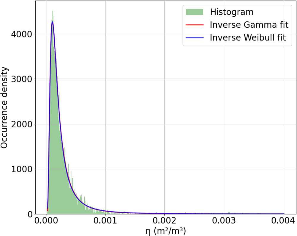
Applying the  $1\varsigma$ rule of the normal distribution, overlaps are observed among the exponential, Rician, and Rayleigh distributions, as well as between the Weibull and gamma, and between the IG and IW distributions. While IG and IW overlap and yield low errors, they remain separate from Weibull and gamma, outperforming them in histogram approximation. In comparison, Weibull and gamma still fit better than Rayleigh, Rician, and exponential distributions. Based on these observations, this study focuses on the IG and IW distributions.
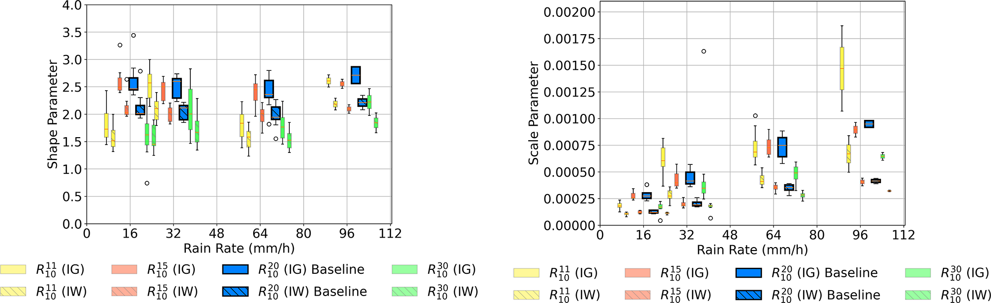
The distinct numerical differences in parameters originate from different mathematical expressions of the two distributions, even though the fitted pdfs overlap substantially, as shown in Figure 6. The parameter variations across rain rates and spatial ranges are summarized in Figure 7. These results demonstrate that both IG and IW distributions exhibit similar behavior. The shape parameter remains within the same range (around 1.5–2.5), indicating the skewed and heavy-tailed nature of the data. In contrast, the scale parameter increases with rain rate (around 0.0002–0.002), indicating greater spread and higher reflectivity ( $\eta$) in rain clutter back-scattering. This is consistent with the Marshall–Palmer drop size distribution, which predicts larger raindrop sizes at higher rain rates [Reference Marshall and Palmer15]. Although the dataset at 98 mm/h was smaller and less reliable due to measurement time limitations, its results are consistent with those at 16, 32, and 66 mm/h for
 $R_{10}^{20}$, showing the same trends in shape and scale.
Histogram & model, TR 30 m, 32 mm/h.

Best-fit model parameters across rain rates and spatial ranges.

Figure 7 Long description
Two grouped box plots compare shape and scale parameters across different rain rates in millimeters per hour. The first box plot on the left illustrates the shape parameter, with the horizontal axis labeled Rain Rate, millimeters per hour, ranging from 0 to 112. The vertical axis labeled Shape Parameter extends from 0.5 to 3.5. Each box represents the interquartile range, with the median marked inside. Whiskers indicate variability outside the upper and lower quartiles and outliers are marked as individual points. The second box plot on the right shows the scale parameter, with the horizontal axis labeled Rain Rate, millimeters per hour, ranging from 0 to 112 and the vertical axis labeled Scale Parameter extending from 0.0000 to 0.0200. Similar statistical elements are present, including medians, quartiles, whiskers and outliers. The legend at the bottom identifies categories such as R subscript 10 superscript 20, IG, R subscript 10 superscript 20, IW, R subscript 10 superscript 20 baseline, R subscript 20 superscript 20, IG, R subscript 20 superscript 20, IW and R subscript 20 superscript 20 baseline. The plots reveal trends in shape and scale parameters, with variability and central tendency differing across rain rates and categories. Higher rain rates tend to show increased variability in scale parameters, while shape parameters remain relatively consistent across categories.
Evaluation against earlier modeling approaches
The results obtained in this study are consistent with the tendencies reported in [Reference Gupta, Varga, Hein and Dallmann1], where a gamma distribution was utilized instead of the IG model considered here. Although the two pdfs are different, their parameter characteristics show similar trends. This can be explained by the statement mentioned in “Inverse-Weibull (IW) distribution” and “Inverse-gamma (IG) distribution” of “Probability distribution functions” section, that the random variables of the gamma and Weibull distributions can be seen as linearization of the IG and IW variables. Since IG and IW provide the best fit, the gamma and Weibull offer quite reasonable, though limited, approximations. Additionally, the IG and IW distributions provide greater flexibility in capturing heavy-tailed behavior, making them advantageous for modeling rain clutter characteristics. The previous work removed outliers, whereas this study contained them while improving resolution in the dense region of the histogram. The validity of this approach is reflected in Figure 4, which shows markedly lower RSS values for the IG and IW models.
Spatial range dependent sensitivity
In this section, different intervals  $[y_{\min},~y_{\max}]$ were considered as ranges under test (
 $R_{y_{min}}^{y_{max}}$). The shape and scale parameters of both IG and IW models for different
 $R_{y_{min}}^{y_{max}}$ ranges are presented in Figure 7. As the range increases, the number of raindrop detections is reduced.
 $R_{y_{min}}^{y_{max}}$ windows with the common near bound
 $y_{min}$ and far bounds extending by 1, 5, 10, and 20 m were examined. For moderately sized spatial ranges (e.g., 5 and 10 m), the estimated parameters exhibit substantial overlap and a clear dependence on rain rate.
In general, there is not much effect of different spatial ranges on the characteristics of the parameters of both models. However, for a narrow spatial range of 1 m, the scale parameter of both models is observed to increase sharply with rain rate. In contrast, for a wider spatial range of 30 m, the scale parameter still increases with rain rate but more gradually. These observations are up for discussion, as fewer detections may lead to a higher influence of outliers.
The authors suspect that these differences arise because the measured reflectivity parameter  $\eta$ from back-scattering by raindrops is inherently exponential. However, the analyzed data is obtained from radar detection lists and is therefore influenced by the sensor’s internal detection algorithm. This processing may include thresholding and range-dependent sensitivity effects, which may suppress weak signal components. As a result, the measured reflectivity statistics are biased by the radar hardware and detection settings. Consequently, the distribution of
 $\eta$ deviates from a purely exponential form and is better described by gamma, IG, or IW models. Since cross-sensor validation is not available in this study, sensor-specific influences cannot be isolated. In [Reference Gupta and Dallmann30], the impact of the sensor detection algorithm on rain back-scattering distributions is investigated through simulation-based analysis. Future work will extend this effort by conducting cross-sensor comparisons to better understand the influence of radar characteristics and detection algorithms on rain clutter statistics.
Furthermore, the IW model exhibits similar parameter trends and data fitting quality as the IG model across ranges and rain rates, reinforcing empirical observations that both models effectively capture the heavy-tailed nature and variability of rain back-scatter. The subtle differences in parameter estimates reflect inherent mathematical distinctions between the models but do not significantly affect their ability to describe the data distribution.
These statistics can be utilized to model rain clutter for various rain rates through interpolation. As already discussed in “Automotive radars” section, modeling automotive radar back-scattering using Mie theory is particularly complex due to the absence of applicable approximations for these radars. Such models can be employed to test measurements for automotive radars in SiL- and HiL-setups, providing an empirical approach to modeling rain back-scattering.
Conclusion
This paper addresses the need for a rain clutter back-scattering model for automotive radar operating at 77 GHz. Although some research exists in this area, much remains unexplored. Radar measurements were conducted in an indoor facility using an irrigation system replicating the Marshall–Palmer drop size distribution. Data were processed using 3-layer robust adaptive binning, and optimized parameter estimation for 119 distributions was performed. The IG and IW distributions exhibited the lowest RSS. These results were further validated based on Monte Carlo simulations.
The shape and scale parameters of both best-fit models were analyzed across varying rain rates, revealing that the shape parameter remains nearly constant, whereas the scale parameter increases with increasing rain rate. These results were compared to the previous analysis reported in [Reference Gupta, Varga, Hein and Dallmann1]. In addition, different spatial ranges were considered for the rain clutter back-scattering models, indicating that varying the spatial range from narrow to wide has minimal impact, with similar patterns observed across ranges. Such analyses can be used to model rain clutter back-scattering in SiL-, HiL-, and ViL-setups. These rain clutter models and test setups provide repeatable scenarios for further research and development in target detection, dynamic range enhancement, and noise reduction for ADAS radar systems.
In future work, the statistics derived from this study may be compared with and complemented by wind velocity distributions. The potential influence of a dominant reflector on rain clutter back-scattering will also be investigated, providing insights into the effect of nearby vehicles on clutter characteristics. Furthermore, an outdoor rain measurement setup is being developed to enable more realistic characterization of rain clutter.
Acknowledgements
This paper was funded by the German Research Foundation (DFG) through the project “P2: Szenarien-basierte Testmethodik für die virtuelle Verifikation und Validierung von KFZ-Radaren” (project number 503852364). The measurement campaign was funded by the German Federal Ministry of Education and Research (BMBF) through project “Virtuelle Validierung – VIVID” (BMBF 16ME0164k). The authors would like to extend their heartfelt thanks to A. Schwind, and S. Buddappagari, former members of the RF and Microwave Research Group at Technische Universität Ilmenau, for conducting the measurements, preprocessing, and providing the data.
Competing interests
The authors report no conflict of interest.

Sonakshi Gupta earned her Bachelor of Technology in Electronics and Communication Engineering from Guru Nanak Dev University, Amritsar, India, in 2018 and her Master of Science in Communication and Signal Processing from Technische Universität Ilmenau in 2022. She is currently a Research Scientist in the Radio Technologies for Automated and Connected Vehicles group at the Thüringer Innovationszentrum Mobilität (ThIMo). Her work focuses on statistical modeling, advanced driver-assistance sensor validation, and sensor virtualization for simulation and testing environments.

Isabella Varga received the B.Sc. and M.Sc. degrees in electrical engineering and information technology from Technische Universität Ilmenau, Ilmenau, Germany, in 2021 and 2023, respectively. She is a Research Scientist in the RF and Microwave Research Group at the Thüringer Innovationszentrum Mobilität, working in the field of radar technologies for automotive applications. Her current research focuses on radar signatures of extended targets based on reflectivity measurements, including modeling, calibration techniques, and signal processing.

Matthias A. Hein (Diploma in Physics 1987, Doctoral dissertation on microwave superconductivity, Dr. rer. nat. 1992, Habilitation 1998) began his academic career at the University of Wuppertal, Germany, researching superconductors for mobile and satellite communications. Following a 13-month British EPSRC Senior Research Fellowship at the University of Birmingham, he joined TU Ilmenau in 2002 as head of the RF and Microwave Research Laboratory. He established the multi-purpose automotive antenna test range “VISTA – Virtual Road Simulation and Test Area” at the Thuringian Center of Innovation in Mobility (ThIMo). His research focuses on antennas and microwaves for intelligent automotive wireless sensor and communication systems, over-the-air testing, and virtual test drives. He has co/authored over 650 publications, delivered over 70 invited talks, and supervised 48 doctoral, 102 master’s, and 91 undergraduate projects, attracting nearly 25 MEUR in research funding. A VDE member since 2003 and an IEEE Senior Member since 2006, he became Director of ThIMo at TU Ilmenau in 2021.

Thomas Dallmann received the Dipl.-Ing. degree in electrical engineering from the RWTH Aachen University, Germany, in 2010 and the Dr.-Ing. degree from the same institution in 2017. From 2016 to 2022, he was with the Fraunhofer-Institute for High Frequency Physics and Radar Techniques FHR, Wachtberg, Germany and led a research group in Aachen, Germany. He is currently Junior Professor at Technische Universität Ilmenau, Germany and is responsible for the Radio Technologies for Automated and Connected Vehicles Research Group. His research is concerned with joint communication, radar sensing networks, and virtual validation of automotive radars.