

Introduction
The recent availability of frequent, high resolution and free remote sensing (RS) images and their derived biophysical products (LAI, fAPAR), added to the valuable information provided by yield maps and crop models, facilitate the development of tools for site specific management of crops. Different ways are used to combine spatialized data with crop models to take into account the spatial variability: (i) defining homogeneous zones from RS images and/or yield maps by classifying the spatialized data (Engel, Reference Engel1997, Pringle et al., Reference Pringle, McBratney, Whelan and Taylor2003) and therefore applying the model to the defined zones after characterization; (ii) spatializing the model according to the soil variability through the definition of soil functional units (Booltink et al., Reference Booltink, Van Alphen, Batchelor, Paz, Stoorvogel and Vargas2001) or (iii) according to a regular grid by re-estimating for each grid cell the inputs of the crop models (soil hydric properties, initial soil water and N conditions) through data assimilation (remote sensing, yield maps) into the crop model (Houlès et al., Reference Houlès, Guérif, Mary, Machet, Moulin and Beaudoin2005). In this paper, we tested a tool based on the third approach which provides spatialized recommendations for N fertilizer applications on wheat, through the use of frequently available high resolution RS images (e.g. SPOT 5, Sentinel 2) and the subsequent assimilation of those data into the STICS crop model. This work is part of the FATIMA H2020 project whose objective is to develop operational decision tools for farmers that must be implemented with limited information.
Materials and methods
Field experiment
The experimental site, situated in south of France (43°48'48‘‘N, 43°48'48‘‘N; Saint-Étienne-du-Grès, France) consisted of a 6 hectares field established with durum wheat (Triticum durum) for two consecutive years. In 2014, the field was sown at the end of October (cv. Dakter) and received two N fertilizer applications, 24 kg N ha−1 as 22:16:0 fertilizer and 108 kg N ha−1 as calcium ammonium nitrate (CAN). In 2015, the field was sown in mid-November with a different variety (cv. Nobilis). The whole field received 44 kg N ha−1 as 22:16:0 fertilizer in January 2016, while the 2nd and 3rd applications (as CAN) were spatially modulated according to the methodology developed in the following sections. The crop was harvested on June 27th 2015 and on July 2nd 2016, in the first and second crop season respectively.
In accordance with the 2015 yield map obtained from the farmer and the LAI dynamics derived from SPOT5 images, five observation plots were set-up, in autumn 2015, to mirror part of the observed variability. In each plot, soil samples were collected (n=3) throughout the season and subsequently analyzed for mineral N content. On each sampling date, soil gravimetric water content was also measured across the soil profile (1 measurement / plot).
Crop development (LAI, biomass, yield) was monitored throughout the season. Plant material was sampled on each plot (n=3), over two rows and along a 50 cm line. Samples were weighed up and subsequently separated between their various fractions (stem, leaves, ears…). Green leaves and stem were passed through a planimeter to estimate the LAI and plant area index (PAI). Wheat yields were calculated after harvest from their components measured on each plot throughout the season.
The crop model
The STICS (Simulateur mulTIdisciplinaire pour les Cultures Standard) crop model simulates crop growth, water and N balance at a daily time-step, and it calculates environmental variables such as N losses (Brisson et al., Reference Brisson, Gary, Justes, Roche, Mary and Ripoche2003). It has been evaluated with good results on large datasets for different crops (Coucheney et al., Reference Coucheney, Buis, Launay, Constantin, Mary and García de Cortázar-Atauri2015) and also in the context of recommending N fertilizer rates for wheat (Houlès et al., Reference Houlès, Mary, Guérif, Makowski and Justes2004). In previous works, the model was parameterized and validated for a wide range of durum wheat varieties around the area (Guillaume, Reference Guillaume, Bergez, Wallach and Justes2011). However, the model has not yet been parameterized and validated for the varieties sown in the field. Hence, for this study, plant parameters of a medium-length cycle variety (cv. Lloyd) were used, as such variety was identified as the most similar STICS default variety to the actual ones in place.
Inverse use of STICS to retrieve soil available water content (AWC) from 2015 observations
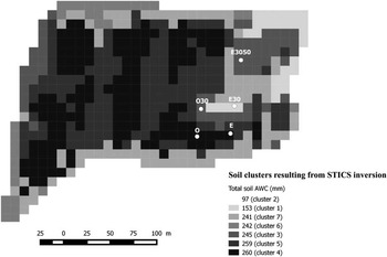
A sequential analysis of six multispectral SPOT 5 images, collected in spring 2015, was carried on to estimate the LAI dynamics during the growing season. The LAI assessment from reflectance was based on a neural network method (Duveiler et al., 2011). A spatialized grid (10×10 m) was built from the pixel definition of SPOT 5 images and was used to re-shape the 2015 yield map provided by the farmer so that all the information could be displayed within the obtained grid. Pixels were classified as 7 homogeneous groups (accounting for more than 75% field variability) whose main source of variability was assumed to be soil AWC (Figure 1), which is known to be one of the main limiting factors in this cropping area.
Spatial distribution of the 7 clusters identified following a clustering analysis on 2015 yield and LAI data. Clusters were then characterized by inverting STICS to retrieve various soil properties which are synthetized here as soil AWC.

As proposed by Varella et al. (Reference Varella, Guérif and Buis2010a), an inversion procedure was then carried on for each group, in a simplified two soil layer approach, to estimate both the soil water content at field capacity (Hfc) for each layer and the thickness of the deeper soil layer. The depth of the upper layer and the maximum soil depth were set to 35 and 120 cm respectively. The soil water content at wilting point (Hwp) was set to a fixed value (0.08 kg kg−1) so that an estimate of soil AWC could be retrieved from the results of the inversion. The GLUE (Generalized Likelihood Uncertainty Estimation) method (Guérif et al., Reference Guérif, Houlès, Makowski and Lauvernet2007) is a Bayesian method that utilizes observations (e.g. LAIs and yields here) to modify a given a priori distribution of chosen model parameter values (from previous runs) into an a posteriori distribution. Mean parameter values from the a posteriori distribution were used to parameterize the model.
Soil texture, organic N content and C:N ratio were averaged values from few field measurements available from the farmer, while dry bulk density, soil carbonate (CaCO3) content and pH were derived from the soil map (Duclos,Reference Duclos1994). Initial water content was set at field capacity at the start of the simulation (1st September 2014) and residual soil nitrate (NO3-N) was set at 40 kg ha−1 in each soil layer to mirror the average values measured in the field in December 2015. Weather data were taken from the information provided by the INRA meteorological station (Avignon, France) located 15 km away from the experimental plots.
In-season estimation of plant density using drone imagery
The spatial variability of LAI was assessed on February 18th, 2016, from an aerial unmanned drone flight which allowed us to secure real time remote sensing acquisition as the Sentinel 2 were not available yet. LAI was estimated by inversion with the PROSAIL model with no prior information (Verger et al., Reference Verger, Vigneau, Chéron, Gilliot, Comar and Baret2014). Estimated values were then re-calibrated from ground measurements using a planimeter (LAI). This LAI information was used to invert STICS to retrieve spatially-distributed plant densities for each homogeneous group. Those densities were within the range of densities observed in the plots (220 to 340 plants m−2).
Optimizing an agro-environmental criterion for spatial N fertilization recommendations
In the area, it is common practice to first apply mineral N fertilizer on wheat during winter, at the three leaves stage. Another two applications usually occur in spring, both at the end of the tillering and the stem elongation stages. The N application rate for the 2nd and 3rd application is usually calculated from an averaged field N balance method (Comifer, 2013), taking into account the crop N requirements and the N supply from the soil. It was assumed that initial soil mineral N was soil cluster-specific and measurements used from a subset of clusters.
In order to compare such N balance method with the variable rate application (VRA) approach, the field was divided into two areas. A small area (=82 cells in the grid, including E3050, E30 and E) was fertilized using a VRA method, while the rest of the field was fertilized according to the results of an averaged field N balance. An agro-environmental criterion, based on agronomic (e.g. yield, protein content) and environmental (e.g. soil mineral N content at harvest) simulation results, was used to determine an optimized N fertilizer rate, for each combination of soil cluster and plant density, over a set of 30 different climatic scenarios. Observed weather data were used to simulate the crop development until the day of the recommendation, while 30 years of historical weather data (1984–2013, SAFRAN data base) were used to predict weather data until harvest. For both N application dates, eleven fertilizer N doses were tested (from 20–100 kg N ha−1, every 10 kg N ha−1). Fertilizer N doses were selected so that the farmer’s gross income could be maximized under the constraint of a 20 kg N ha−1 threshold for the residual soil mineral N content after harvest.
Post-harvest evaluation of the approach
Our approach was assessed over five grid cells, corresponding to the five observation plots set up in the field. Two of them (O and E) belonged to one of the most representative (29%) soil cluster (cluster 4, soil AWC=260 mm). Another two plots (O30 and E3050) belonged to cluster 3 (AWC=245 mm), quite present in the eastern part of the field. Finally, the E30 plot was set up in a quite atypical area in the field, with a high proportion of sand observed in the upper soil layer, and was identified as part of the soil cluster 1 (AWC=153 mm, Figure 1). Simulation outputs were considered for each plot and root mean square errors (RMSE) were calculated for each simulated variables whenever observations were available.
In this paper, to stress out the interest of addressing the spatial variability of soil and crop dynamics, we considered three different modelling scenarios differing by the level of knowledge on the spatial distribution of soil and crop properties:
-
∙ an averaged field approach (= field N balance), where soil model inputs were averaged from the most representative cluster (O and E plots) to mimic the conventional field-based nutrient management approach;
-
∙ an ‘operational’ approach, where the model was fed with basic information that could be reasonably asked to farmers or easily obtained from crop model inversion using RS data (e.g. LAI) and yield maps, where soil AWC was estimated for each soil layer by inverting STICS and where soil water content was initialized at field capacity;
-
∙ an ‘ideal’ approach where the model was fed with as much knowledge as we could, where soil AWC was determined for each soil layer using pedotransfer functions (Wösten et al., Reference Wösten, Lilly, Nemes and Lebas1999) and where soil water content was initialized to match observations.
Both simulations were initialized on a plot-scale basis, in terms of mineral N, as we intend, in the future, to retrieve spatialized soil N data from the inversion of STICS with RS data.
Results and discussion
Off-line estimation of soil AWC and in-season estimation of plant density
Soil AWC estimates for each soil cluster and their spatial distribution are shown in Figure 1.
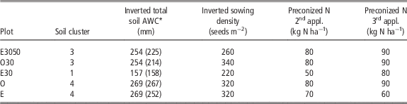
Those values were similar to the ones predicted by pedotransfer functions (Wösten, Reference Wösten, Lilly, Nemes and Lebas1999) based on soil texture observations (Table 1). In terms of plant densities, retrieved results reflected a lower plant development during the whole growing period and led to lower yields (Figures 1 and 2).
Key parameterization choices, in terms of soil hydric properties and crop management, for both the ‘operational’ and ‘ideal’ simulations

* in bracket are given the estimation from texture observation and pedotransfer function
Ability of STICS to simulate soil and crop status
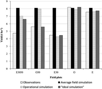
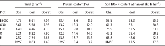
Our ‘averaged field’ simulation was unable to match the yield variability observed between plots (Figure 2). Conversely, both the ‘operational’ and ‘ideal’ simulations gave good estimates of yields for the E30, O and E plots. However, they were unable to reproduce the crop behavior for the E3050 plots, where winter and spring LAI observations indicated a poor crop establishment which could not be offset by tillering (Figure 2 and Table 2). The impact of a poor crop establishment on the resulting yield seems difficult to simulate using STICS and the chosen cultivar parameters.
Yield observations and simulations, in 2016, for the 5 reference plots.

Agronomical and environmental outputs from STICS calculated for both the ‘ideal’ and the ‘operational’ simulations. Field observations are also provided for comparisons

There were differences between the ‘operational’ and ‘ideal’ simulations regarding their ability to simulate the wheat yield at harvest on the O30 plot. Indeed, simulated yield from the ‘ideal’ simulation are similar to the one measured in the field whereas the ‘operational’ simulation over-estimates the same yield by 2.4 t ha−1 (Figure 2 and Table 2). Calculated water and N stress index show that an early water stress in the ‘ideal’ simulation accelerated the LAI drop during the plant senescence phase, hence offsetting a previous high crop development phase (Figure 3). In the ‘operational’ simulation, there is no such early water stress and the yield for the O30 plot remains nearly as high as the ones registered for the two high yielding plots (O and E). The difference in water stress a result of the initialization. In the operational case the soil water content was prescribed to field capacity, whereas in the optimal case, initialization was done to match the first soil moisture measurements.
Dynamic of the observed and simulated LAI during the 2016 crop season for (left) the ‘operational’ simulation and for (right) the ‘ideal’ simulation.

Overall, the simulated LAI profiles tend to match observed LAIs at the start of the growing season. However, the E30 and E3050 plots are not well represented around the LAI peak phase (Figure 3) because of low NO3-N initialization values and plant density.
Agronomical and environmental outputs from the STICS model show its ability to provide good yield predictions, as was shown by Coucheney et al. (Reference Coucheney, Buis, Launay, Constantin, Mary and García de Cortázar-Atauri2015). However, the same authors showed that the model may struggle to provide good estimates of the wheat protein content and soil N status, which is clearly shown here by the high RMSE values calculated for the wheat protein and soil NO3-N content at harvest (Table 2). The comparison between both the ‘ideal’ and ‘operational’ simulations shows similar results for wheat protein and soil NO3-N content at harvest, except for the O30 plot whose simulated protein content in grain and soil NO3-N at harvest were significantly lower for the ‘operational’ simulations (Table 2).
Interest of variable rate N fertilizer applications
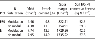
Three field plots (E3050, E30 and E) were modulated, in terms of N fertilization, to optimize their agronomic potential and minimize the environmental impact. However, for the E3050 plot, the modulation process led to the same results as the N balance approach used in the unmodulated area. For the other two plots, we compared simulations from both the ‘N modulation’ and ‘field N balance’ scenarios to assess the impact of the VRA approach on some agronomical and environmental criteria (Table 3).
Comparison between the ‘spatialized N modulation’ and the ‘field N balance’ scenarios for two plots.. Simulation results are based on the ‘ideal’ soil parameterization

Modulating the crop N management had little effect on yields (Table 3). However, the gross margin was improved by 8.9% for low productivity soils (E30 simulation) thanks to a reduction in the N fertilizer costs, while it remains unchanged in a more productive area (E simulation) where the simulated yield was similar to the field average value. Modulation had a major impact on soil NO3-N content at harvest with a simulated 13% and 28% decrease for the E30 and E plots respectively (Table 3), hence lower risks of N leaching over the autumn and winter season when bare soils are close to field capacity.
In this work, only data (LAI, yield) used from one growing season to estimate some permanent soil properties, assuming that the observed variability was the result of the spatial distribution of soil hydric properties. Varella et al. (Reference Varella, Guérif, Buis and Beaudouin2010b) showed that such properties can be better estimated by the inversion of crop models on a single year, when water stress effects occur. The encountered soil/climate combination was found appropriate to describe soil variability and then a multiyear data set is not necessarily provide better soil characterization.
The STICS model appeared to be appropriate to simulate water stress impact on crop growth and yield. The soil AWC appeared to be well estimated thanks to a dry 2015 year, and the effect of water stress on the yield in plot E30, which had the lowest AWC, was well characterized. In that case the N recommendation led to a clear improvement in the gross margin. The STICS simulation also appeared to be very sensitive to the N initialization, which will be a problem in operational context as the soil N content would be difficult to map. Early detection on LAI dynamic or on spectral indices linked to the chlorophyll content should be better explored to reduce such source of uncertainty.
Conclusions
This work demonstrates the value of using data assimilation in a mechanistic crop model such as STICS for spatial management of N fertilization. Especially, it is shown that, with the monitoring of foliar development during a crop cycle and the use of spatialized yield data, it is possible to map soil AWC. However, it is advisable to have a climatic year, during which the water stress is expressed differently within the field. For the second N supply, the growth of the vegetation wat not sufficient to express N deficiencies or water stresses. If the study has shown that the estimation of AWC and resulting water dynamics are well addressed by the proposed methodology, the impact of a poor crop establishment on yields, expressed on the foliar development, was not well simulated by STICS. Some work should be done to better parameterize the model. Another remaining issue is the characterization of the initial soil N content which has a strong impact on STICS simulations and thus requires an accurate estimation. A finer analysis of RS information is required to detect N stresses. This work shows the need to have time series with a good frequency of acquisition to better detect plant stresses. This is now possible with new Earth observation missions such as Sentinel 2.
Acknowledgements
This project was funded by EU Grant 633945—FATIMA—H2020-SFS-2014-2015/H2020-SFS-2014-2