2 Mathematical formulation

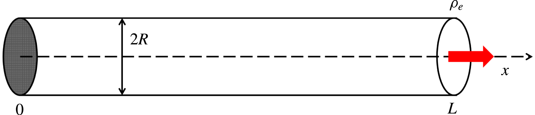
We study the slow viscous drainage flow of a single phase compressible fluid from a long small capillary with one end sealed by a solid surface (figure 1). The capillary has an inner radius $R$ and length $L$ , with $R\ll L$ . The fluid stored in the tube is either a gas or a liquid, and it is initially at rest with a density  $\unicode[STIX]{x1D70C}_{i}$ with both ends closed. The capillary tube is embedded in a large bath of the same compressible fluid maintained at a density $\unicode[STIX]{x1D70C}_{e}$ slightly lower than $\unicode[STIX]{x1D70C}_{i}$ . At $t=0$ , the end of the tube at $x=L$ is opened fully, and the density at the exit is maintained at  $\unicode[STIX]{x1D70C}_{e}$ at all times thereafter. Volumetric expansion causes the fluid to drain from the tube through the opening. The density difference $\unicode[STIX]{x1D70C}_{i}-\unicode[STIX]{x1D70C}_{e}$ is assumed to be small relative to the initial density, $\unicode[STIX]{x1D6FF}=(\unicode[STIX]{x1D70C}_{i}-\unicode[STIX]{x1D70C}_{e})/\unicode[STIX]{x1D70C}_{i}\ll 1$ , and temperature variation is negligible. The Mach number defined as the ratio between a characteristic fluid velocity $V$ and the speed of sound $c$ for this drainage flow is assumed to be small, $Ma=V/c\ll 1$ . Thus, the continuity and the compressible Navier–Stokes equations (Chorin & Marsden Reference Chorin and Marsden1992) can be linearized around the final equilibrium state $(\unicode[STIX]{x1D70C},\boldsymbol{v})=(\unicode[STIX]{x1D70C}_{e},0)$ so that (Morse & Ingard Reference Morse and Ingard1968; Temkin Reference Temkin1981)

where the density perturbation $\unicode[STIX]{x1D70C}^{\prime }=\unicode[STIX]{x1D70C}-\unicode[STIX]{x1D70C}_{e}$ ; $p^{\prime }$ is the pressure perturbation; $\boldsymbol{v}^{\prime }$ is the velocity perturbation which is assumed to be axisymmetric; $\unicode[STIX]{x1D707},\unicode[STIX]{x1D707}_{b}$ are the shear and bulk viscosities of the fluid, respectively. It can be shown from (2.1) and (2.2) that the density perturbation is governed by a damped wave equation (Morse & Ingard Reference Morse and Ingard1968; Temkin Reference Temkin1981)

where the diffusion coefficient $D_{\unicode[STIX]{x1D70C}}=(\unicode[STIX]{x1D707}_{b}+4\unicode[STIX]{x1D707}/3)/\unicode[STIX]{x1D70C}_{e}$ characterizes the diffusion of a small density disturbance. When the sealed end is a rigid sound reflecting surface, the boundary and initial conditions for the density are

No wall condition for density needs to be specified and the density value on the wall is determined by the solution itself (see § 3 below). For the present problem, the mass flow rate at the tube exit ${\dot{m}}_{e}(t)$ can be computed once the instantaneous density distribution is obtained from the above initial-boundary-value problem without the need for the explicit knowledge of the corresponding velocity field, as the integral of the continuity equation over the entire tube gives

Relation (2.6) is general for a tube with a sealed end, not limited to the linearized problem considered here. It simply states that the mass flow rate from a half-sealed tube equals to the time rate of decrease of the fluid mass inside the tube.

Figure 1.

Drainage flow from a semi-closed capillary tube. The initial density is $\unicode[STIX]{x1D70C}_{i}$ ; and the exit density is $\unicode[STIX]{x1D70C}_{e}$ .

To understand the characteristics of viscous compressible flow in small capillaries, the velocity field will be computed once the density distribution for the linearized flow is obtained. From the Helmholtz decomposition theorem (Aris Reference Aris1989; Leal Reference Leal2010; Panton Reference Panton2013), the velocity field $\boldsymbol{v}^{\prime }$ can be decomposed into the sum of an irrotational part $\boldsymbol{v}_{IR}^{\prime }$ and a rotational part $\boldsymbol{v}_{RT}^{\prime }$ ,

where the irrotational part is a potential flow and the rotational part is solenoidal (incompressible):

In the above, $\unicode[STIX]{x1D6F7}$ is the scalar velocity potential for the irrotational flow. These two parts of the velocity field are called the longitudinal mode and transverse mode respectively in the acoustic literature (Morse & Ingard Reference Morse and Ingard1968; Temkin Reference Temkin1981). In the linear theory studied here, the two modes are only coupled through the no-slip condition on the tube wall for the total velocity $\boldsymbol{v}^{\prime }$ ,

The irrotational velocity can be determined from the continuity equation which now takes the form

since $\unicode[STIX]{x1D735}\boldsymbol{\cdot }\boldsymbol{v}_{RT}^{\prime }=0$ . At $x=0,\boldsymbol{v}_{IR}^{\prime }=0$ .

The solenoidal velocity $\boldsymbol{v}_{RT}^{\prime }$ is governed by the equations for an incompressible flow, which can be expressed in terms of the incompressibility condition and the linearized vorticity diffusion equation

where the kinematic viscosity $\unicode[STIX]{x1D708}_{e}=\unicode[STIX]{x1D707}/\unicode[STIX]{x1D70C}_{e}$ . The solenoidal velocity is solely driven by the no-slip condition imposed on the overall velocity, equation (2.10).

The linearized problem formulated here can be considered as the leading-order solution in an asymptotic expansion in terms of the small density change $\unicode[STIX]{x1D6FF}=(\unicode[STIX]{x1D70C}_{i}-\unicode[STIX]{x1D70C}_{e})/\unicode[STIX]{x1D70C}_{i}\ll 1$ . Thus, the neglected terms will be of the order of $\unicode[STIX]{x1D6FF}^{2}$ . It should be pointed out that the exit boundary condition of a fixed density (or pressure) is frequently used for tube flows and it is an idealization for the interaction between the flow inside the tube and the flow outside of the tube. Imposing an appropriate outlet boundary condition for the unsteady Navier–Stokes equations is generally a non-trivial matter (Gresho Reference Gresho1991; Poinsot & Lele Reference Poinsot and Lele1992; Sani & Gresho Reference Sani and Gresho1994). An exit region of the size of a few tube diameters characterizing the influence on the tube flow from the fluid outside of the tube is expected (Gottlieb & Bird Reference Gottlieb and Bird1979). Since this exit region is small in comparison to the length of the tube, equation (2.6) indicates that the exit effect has a limited influence on the mass flow rate. Numerical solution of the linearized Navier–Stokes equations for drainage flow into a large finite reservoir is carried out in this study to verify whether the fixed density exit boundary condition is an appropriate approximation for drainage flow to a large reservoir. It is also noted that the problem of compressing a prefilled gas during liquid filling of a blind pore is quite different from the flow considered here, as a moving boundary condition must be imposed at the gas–liquid surface which also involves surface tension effect (Hultmark, Aristoff & Stone Reference Hultmark, Aristoff and Stone2011).

3 Density relaxation and the irrotational velocity field

It is well known that when solving the Navier–Stokes equations, the only boundary condition required on the solid–fluid surface is the no-slip condition for the velocity and no boundary condition for the pressure or the density is needed (Scarton & Rouleau Reference Scarton and Rouleau1973; Monkewitz Reference Monkewitz1979). Since the linearized Navier–Stokes equations are being solved here, it is also expected that we only need to impose the no-slip condition for the velocity on the capillary wall without the need to specify a boundary condition for the density. This is confirmed by the solution of the damped wave equation for the density shown in detail below.

It is first noted that, in general, any function $\unicode[STIX]{x1D70C}^{\prime }(r,x,t)$ can be expressed as the sum of a part independent of $r$ and a part that vanishes on the capillary wall,

where the $r$ -dependent part $\unicode[STIX]{x1D70C}_{2}^{\prime }(r,x,t)$ vanishes on the tube wall, $\unicode[STIX]{x1D70C}_{2}^{\prime }(R,x,t)=0$ . It turns out that when the method of separation of variables is used to solve the initial-boundary-value problem for the density perturbation (2.3)–(2.5), the $r$ -independent part of the solution $\unicode[STIX]{x1D70C}^{\prime }(R,x,t)$ naturally corresponds to the eigenvalue zero, whilst the $r$ -dependent part $\unicode[STIX]{x1D70C}_{2}^{\prime }(r,x,t)$ corresponds to the non-zero eigenvalues that are related to the root of the Bessel function $\text{J}_{0}$ . In other words, the boundary value for the density is determined by the eigenvalue problem arising from the separation of variables. Thus, there is no need to specify the wall condition for the density and the density value on the wall is determined by the solution itself. It is observed that when studying inviscid compressible flows in tubes, it is customary to assume that the density is uniform over the cross-section of the tube. Even with this assumption, density is still part of the solution, and it cannot be prescribed a priori (see any textbook on gas dynamics). In the current work, we make no assumption about the uniformness of the density over the tube cross-section or the value of the density on the tube wall. The value of the density on the wall can be obtained from the solution itself, consistent with fluid mechanics theory.

The complete solution for the density perturbation is given by

where

In the above, $\text{J}_{n}$ is the $n$ th-order Bessel function of the first kind; $\text{J}_{0}^{\prime }$ is the first derivative of $\text{J}_{0}$ ; and $\unicode[STIX]{x1D6FD}_{m}$ are the roots of $\text{J}_{0}$ . The floor function gives the integer less than or equal to its argument. The single-sum series in the solution (3.2) is independent of the radial coordinate  $r$ , where $N_{d}$ is an integer such that $\unicode[STIX]{x1D714}_{n}$ becomes imaginary when $n>N_{d}$ . $N_{d}=O(10^{7})$ for metre-length tubes, $L=1m$ , and typical fluids properties $c=400~\text{m}~\text{s}^{-1}$ , $D_{\unicode[STIX]{x1D70C}}=10^{-5}~\text{m}^{2}~\text{s}^{-1}$ . The part with $n>N_{d}$ is purely diffusive (non-oscillatory). The decay rate for this diffusive portion of the series is approximately $\exp (-2\unicode[STIX]{x1D6FE}_{n}t)$ or $\exp (-c^{2}t/D_{\unicode[STIX]{x1D70C}})$ , whichever is smaller. For $c=400~\text{m}~\text{s}^{-1}$ , $D_{\unicode[STIX]{x1D70C}}=10^{-5}~\text{m}^{2}~\text{s}^{-1}$ , $\exp (-c^{2}t/D_{\unicode[STIX]{x1D70C}})\sim \exp (-10^{9}t)$ , which is an extremely fast decay; whilst $\exp (-2\unicode[STIX]{x1D6FE}_{n}t)$ always decays faster than the terms with $n\leqslant N_{d}$ . Thus, the purely diffusive part of the series can be neglected in the calculations for large times due to their fast decay.

The double-sum series in the solution (3.2) contains the $r$ -dependence of the density profile which vanishes on the tube wall. The slowest decaying mode in the double-sum series is the $(n,m)=(0,1)$ mode. A Taylor series expansion for small tube radius (more precisely for small ratios of $R/L$ ) gives, to the leading order,

$K_{01}^{+}$ is the aeroacoustic mode, which decays with a rate of $\exp (-c^{2}t/D_{\unicode[STIX]{x1D70C}})$ , independent of the length and the radius of the tube; and as shown above, it decays fast as $\exp (-10^{9}t)$ . $K_{01}^{-}$ is the highly damped viscous mode for very small tubes. For a micron-size tube $R=10^{-6}~\text{m}$ and $D_{\unicode[STIX]{x1D70C}}=10^{-5}~\text{m}^{2}~\text{s}^{-1}$ , $K_{01}^{-}=-5.81\times 10^{7}~\text{s}^{-1}$ . Thus, for micron-size tubes, after a very short time, of the order $O(10^{-7}~\text{s})$ , the double-sum series in (3.2) quickly decays to zero and the density relaxes to a profile uniform over the tube cross-section with the density perturbation given by the single-sum series. This density relaxation occurs even faster for nano-size tubes. In other words, the density wave quickly approaches the plane wave solution in a small tube. This fast relaxation of the density in the transverse direction is due to strong transverse viscous diffusion (strong transverse damping effect) in small capillaries. It should be pointed out that the fast density relaxation in the transverse direction is subject to the large length-to-radius ratio constraint for the capillary tube, as (3.10), (3.11) are derived under such conditions. The relaxed density profile has also been confirmed by numerical solution of the linearized Navier–Stokes equations (§ 6).

The transversely relaxed density perturbation is given by

after neglecting the fast decaying purely diffusive modes. The relaxed density is independent of the radial coordinate $r$ as well as the tube radius $R$ . Equation (3.12) shows that in small capillary tubes, while any density variation in the cross-sectional direction is smoothed out very quickly, viscous damping of the longitudinal variation of density is extremely slow, on the diffusive time scale $L^{2}/D_{\unicode[STIX]{x1D70C}}$ (since $\unicode[STIX]{x1D6FE}_{n}\sim D_{\unicode[STIX]{x1D70C}}/L^{2}$ ). Equation (3.12) is a damped standing wave solution for the density, with a node at the exit $x=L$ and an antinode at the sealed end $x=0$ . Upon the opening of the tube exit, an inward propagating rarefaction wave is initiated and this acoustic wave travels towards the sealed end. Once reflected from the end of the tube, the rarefaction wave travels towards the exit to complete the rarefaction phase. The wave then becomes compressive as it travels back towards the sealed end once again, getting reflected from the end, travelling towards the exit and finally completing the compression phase once it reaches the exit. The amplitude of the wave decays continuously as the wave goes through the rarefaction and then compression phase in each cycle. Contrary to common belief, the slow damping of the wave amplitude gives the standing acoustic wave a surprisingly long life which is of the diffusive time scale $L^{2}/D_{\unicode[STIX]{x1D70C}}$ . This result is consistent with recent findings that an acoustic impulse in a highly confined compressible fluid can create a long time memory effect for the compressible fluid (Hagen et al. Reference Hagen, Pagonabarraga, Lowe and Frenkel1997; Felderhof Reference Felderhof2010; Frydel & Diamant Reference Frydel and Diamant2012).

For the plane wave solution of the density (3.12), the irrotational velocity obtained from the continuity equation becomes $\boldsymbol{v}_{IR}^{\prime }=v_{x,IR}^{\prime }(x,t)\boldsymbol{e}_{x}$ , with

The solution satisfies the boundary condition at the sealed end, $x=0$ , $\boldsymbol{v}_{IR}^{\prime }=0$ . Thus, the irrotational part of the instantaneous velocity is independent of radial coordinate $r$ as well as the tube radius $R$ ; and it scales with $c(\unicode[STIX]{x1D70C}_{i}-\unicode[STIX]{x1D70C}_{e})/\unicode[STIX]{x1D70C}_{e}$ , not with the viscous velocity scale from the Poiseuille’s law.

4 The solenoidal velocity field

The solenoidal velocity is axisymmetric and driven by the no-slip condition on tube wall for the overall velocity, equation (2.10). On the sealed end at $x=0$ , the irrotational velocity is zero; thus, the solenoidal velocity satisfies the no-slip condition there. At the exit $x=L$ , the perturbation pressure is zero. With these boundary conditions, it is difficult to obtain an analytical solution for the solenoidal velocity even for the plane wave solution of the irrotational velocity. Thus, we choose to find the solenoidal velocity numerically using the software package COMSOL (COMSOL 2016). The linearized unsteady incompressible Navier–Stokes equation was solved subject to the above boundary conditions using fully coupled PARDISO direct solver and Jacobian update on every time step. The generalized alpha time stepping method was used with maximum time step set as $1/256$ of the period. Quad elements are generated using the mapped mesh tool, dividing the radius of the tube into elements spaced exponentially with finer mesh distributed near the tube wall in order to capture the Stokes boundary layer, and the tube length is divided into linearly spaced elements. Second-order elements for the velocity components and linear elements for the pressure field are used. Mesh refinements are performed to ensure convergence of the numerical results.

It is first noted that for the relaxed density, the irrotational velocity is a plane wave solution. Thus, the radial component of the solenoidal velocity must be zero on the tube wall. The instantaneous volumetric flow rate of the solenoidal velocity over any cross-section of the tube $Q_{RT}$ is identically zero at any time, since $\unicode[STIX]{x1D735}\boldsymbol{\cdot }\boldsymbol{v}_{RT}^{\prime }=0$ with zero radial velocity on the tube wall implies that $Q_{RT}(x)=\text{const.}=Q_{RT}(0)=0$ . This also implies that the solenoidal velocity component $v_{x,RT}^{\prime }$ must experience a reversal on any cross-section. Thus, the solenoidal velocity does not contribute to the mass flow rate and the role of the solenoidal velocity is to enforce the no-slip condition on the tube wall for the overall velocity.

Figure 2.

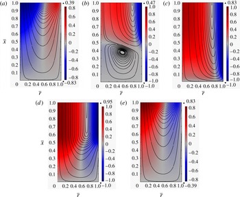
Instantaneous streamlines for the solenoidal velocity with $L=1~\text{m}$ , $R=50~\unicode[STIX]{x03BC}\text{m}$ , for the first half-cycle (rarefaction), starting with $t=68~\text{s}$ . $\unicode[STIX]{x1D70C}_{i}=136.78~\text{kg}~\text{m}^{-3}$ , $\unicode[STIX]{x1D70C}_{e}=132.68~\text{kg}~\text{m}^{-3}$ , $\unicode[STIX]{x1D707}=1.99\times 10^{-5}~\text{Pa}~\text{s}$ , $D_{\unicode[STIX]{x1D70C}}=4.82\times 10^{-5}~\text{m}^{2}~\text{s}^{-1}$ . Period $T=0.0125~\text{s}$ . Colour bars indicate velocity, negative values indicate gas flows into the tube. Flow rate at any cross-section is zero. (a) $t=68~\text{s}$ ; (b) $t=68~\text{s}+T/8$ ; (c) $t=68~\text{s}+T/4$ ; (d) $t=68~\text{s}+3T/8$ ; (e) $t=68~\text{s}+T/2$ .

Figure 2 shows a sequence of the instantaneous streamlines for the solenoidal velocity for a tube with $L=1m$ , $R=50~\unicode[STIX]{x03BC}\text{m}$ during the first half-cycle of density oscillation (rarefaction) starting at $t=68~\text{s}$ . In the figure, $\bar{r}=r/R;\bar{x}=x/L$ . While the example is specifically for methane at pressure of 25 MPa and temperature at $80\,^{\circ }\text{C}$ , the flow characteristics remain qualitatively the same for common compressible fluids such as air at a lower pressure and temperature. The five instants shown are $1/8$ period apart, starting from the beginning of the cycle. Red and blue colours correspond to positive and negative streamwise solenoidal velocities, respectively. At $1/8$ period, a weak vortex appears near the end of the tube (figure 2 b). However, as time increases, this vortex is squeezed towards the end of the tube and it disappeared altogether just before the $1/4$ period mark (figure 2 c). At the end of the half-cycle, the rarefaction wave has travelled back to the tube exit and the solenoidal velocities almost become the mirror images of those at the beginning of the cycle (figure 2 e), with the fluid at the centre portion of the tube moving out of the tube and in the near wall region moving into the tube. The acoustic wave turns around and travels inward as a compressive wave, with the stream-line patterns essentially being the reverse of the sequence shown in figure 2. It must be emphasized that these instantaneous streamlines correspond to the solenoidal velocity field, not the total velocity field.

Figure 3.

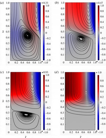
Effect of tube size. Streamlines for the solenoidal velocity field with length $L=1~\text{m}$ at time $t=68+T/8$ , $T=0.0125~\text{s}$ is the period. (a) $R=100~\unicode[STIX]{x03BC}\text{m}$ ; (b) $R=50~\unicode[STIX]{x03BC}\text{m}$ ; (c) $R=30~\unicode[STIX]{x03BC}\text{m}$ ; (d) $R=10~\unicode[STIX]{x03BC}\text{m}$ . $\unicode[STIX]{x1D70C}_{i}=136.78~\text{kg}~\text{m}^{-3}$ , $\unicode[STIX]{x1D70C}_{e}=132.68~\text{kg}~\text{m}^{-3}$ , $\unicode[STIX]{x1D707}=1.99\times 10^{-5}~\text{Pa}~\text{s}$ , $D_{\unicode[STIX]{x1D70C}}=4.82\times 10^{-5}~\text{m}^{2}~\text{s}^{-1}$ .

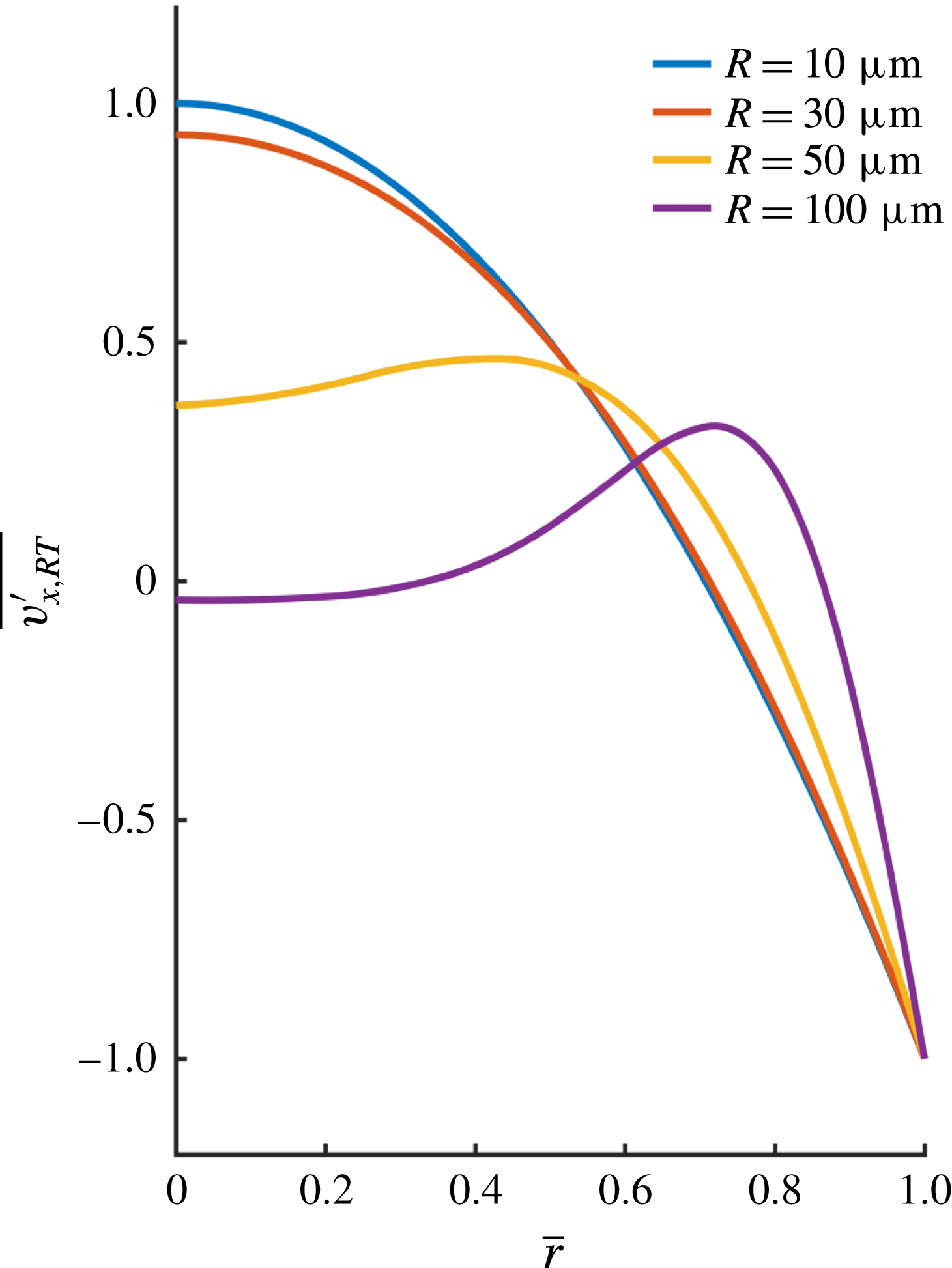
Figure 3 shows the effect of tube size on the instantaneous streamlines of the solenoidal velocity field for $R=100~\unicode[STIX]{x03BC}\text{m}$ , $50$ , $30$ , $10~\unicode[STIX]{x03BC}\text{m}$ at the instant of $1/8$ period. The corresponding instantaneous streamwise velocity profiles at the exit plane are shown in figure 4. It is observed that for large tubes ( $100$ , $50$ , $30~\unicode[STIX]{x03BC}\text{m}$ ), there is a weak vortex near the end of the tube to accommodate the no-slip condition at the end surface. This vortex becomes weaker as the tube radius is reduced. The vortex disappears (or is too weak to be plotted) when the radius is reduced to $10~\unicode[STIX]{x03BC}\text{m}$ . For larger tubes, the streamwise solenoidal velocity ${v^{\prime }}_{x,RT}$ is the classical Stokes solution driven by an oscillatory boundary (figure 4 a). A Stokes boundary layer is formed near the tube wall, with a thickness of the order of $\unicode[STIX]{x1D6FF}_{St}\approx \sqrt{2\unicode[STIX]{x1D708}_{e}/\unicode[STIX]{x1D714}_{0}}=\sqrt{4L\unicode[STIX]{x1D708}_{e}/(\unicode[STIX]{x03C0}c)}$ , which is independent of the radius and it is approximately $18~\unicode[STIX]{x03BC}\text{m}$ for the cases shown in figure 4. As the tube radius is reduced, the ratio between the Stokes layer thickness and the radius becomes larger (figure 4 b), as the Stokes layer occupies a larger portion of the tube, and the streamwise solenoidal velocity spreads over the entire tube cross-section for very small radii (figure 4 c,d). Due to the reversal of ${v^{\prime }}_{x,RT}$ discussed earlier, the centreline velocity is always in the opposite direction of the wall velocity. A consequence of the Stokes layer spreading over a larger portion of the tube is that the centreline velocity for the solenoidal velocity ${v^{\prime }}_{x,RT}$ must increase in order to satisfy the condition of zero flux $Q_{RT}(x)=0$ . In the small radius limit, ${v^{\prime }}_{x,RT}$ approaches a parabolic shape, with the centreline and wall velocity having the same magnitude but opposite signs (e.g. $10~\unicode[STIX]{x03BC}\text{m}$ tube, figure 4 d).

Figure 4.

Dimensionless streamwise solenoidal velocity profile $\overline{v_{x,RT}^{\prime }}=v_{x,RT}^{\prime }/|v_{x,IR}^{\prime }|$ at the tube exit, $\bar{r}=r/R$ , from large tubes to smaller tubes, corresponding to the cases shown in figure 3. The Stokes layer occupies a larger portion of the tube as the radius is reduced.

5 Drainage rate and the mechanism of fluid production

Draining a compressible fluid from a small capillary with a sealed end is a process of transporting and subsequent extinguishment of the density perturbation initiated at the tube exit. Two transport mechanisms are involved: sonic transport by acoustic wave and diffusive transport by longitudinal density gradient. While the acoustic wave transmits the density perturbation, it also tends to maintain such a disturbance. It is the longitudinal diffusion that damps the acoustic wave and produces fluid drainage.

The instantaneous mass flow rate at the exit can be computed from the density profile by integrating the continuity equation

Thus, the mass flow rate oscillates in time and it experiences intervals of positive values (production) followed by negative values (suction) within each period of oscillation. Since the cycle starts from the production phase, a continuous amplitude decay in time ensures that there is a net positive mass production after each oscillation period. The drainage rate $\hat{{\dot{m}}}_{e}(t)$ is the period-averaged mass flow rate at the exit and it is given by

When $t\gg T$ , the higher modes (large $n$ ) experience large exponential decays and their contributions to the drainage rate are negligible. The lower modes can be approximated by the leading term in the Taylor series expansion for $1-\exp (-\unicode[STIX]{x1D6FE}_{n}T)$ . Thus, the leading-order expression for the drainage rate is given by

where $M_{L}=\unicode[STIX]{x03C0}R^{2}L(\unicode[STIX]{x1D70C}_{i}-\unicode[STIX]{x1D70C}_{e})$ is the total amount of producible fluid from the capillary for a given density drop $\unicode[STIX]{x1D70C}_{i}-\unicode[STIX]{x1D70C}_{e}$ ; $N$ is the cutoff integer so that $\unicode[STIX]{x1D6FE}_{n}T=(2n+1)^{2}\unicode[STIX]{x03C0}^{2}D_{\unicode[STIX]{x1D70C}}/2cL<1$ for $n<N$ ( $N\approx 10^{3}$ for $D_{\unicode[STIX]{x1D70C}}\approx 10^{-5}~\text{m}^{2}~\text{s}^{-1}$ , $L=1~\text{m}$ ). Since the period $T$ for a metre-long tube is typically of the order of 0.01 s, the drainage rate expression (5.3) can be used virtually for all times of interest. A period-averaged drainage speed corresponding to the drainage rate can be defined as

Thus, fluid is drained from the capillary in an oscillatory huff-n-puff pumping process driven by the decay of the standing acoustic wave. On a time scale much larger than the period of oscillation, the drainage rate $\hat{{\dot{m}}}_{e}(t)$ is determined by the slow diffusive time scale $L^{2}/D_{\unicode[STIX]{x1D70C}}$ and it is independent of the oscillation frequency. The drainage rate (5.3) is proportional to the diffusion coefficient $D_{\unicode[STIX]{x1D70C}}=(\unicode[STIX]{x1D707}_{b}+4\unicode[STIX]{x1D707}/3)/\unicode[STIX]{x1D70C}_{e}$ , which is related to the combined bulk and shear viscosities $\unicode[STIX]{x1D707}_{b}+4\unicode[STIX]{x1D707}/3$ , and the square of the tube radius $R^{2}$ . If we set the bulk viscosity to zero as in Stokes’ hypothesis, then the diffusion coefficient $D_{\unicode[STIX]{x1D70C}}$ is essentially the kinematic viscosity of the fluid. Thus, despite the overall velocity satisfying the no-slip condition on the capillary wall, the flow shows a slip-like mass flow rate which is also proportional to the fluid’s kinematic viscosity. This is a fundamental departure from the classical Poiseuille’s law which gives a drainage rate inversely proportional to the kinematic viscosity and proportional to the quartic power of the tube radius $R^{4}$ . The proportionality of the drainage rate to the kinematic viscosity of the fluid is due to the fact that the drainage process is controlled by the diffusion of the density which has a diffusion coefficient proportional to the fluid’s kinematic viscosity. The above findings can also be understood in terms of the velocity field: the solenoidal velocity does not contribute to the mass flow rate; and the irrotational velocity is uniform in any cross-section for the relaxed density profile which gives rise to the slip-like mass flow rate, even though the overall velocity does not slip on the tube wall.

The drainage speed $V_{e}(t)$ scales with the diffusive velocity scale $D_{\unicode[STIX]{x1D70C}}/L$ . This drainage speed is the average Lagrangian velocity for the fluid particles that have exited the tube during one period of oscillation, and it differs significantly from the instantaneous Eulerian velocity at the tube exit. The instantaneous velocity scales with $c(\unicode[STIX]{x1D70C}_{i}-\unicode[STIX]{x1D70C}_{e})/\unicode[STIX]{x1D70C}_{e}$ , much faster than the drainage speed. Despite the high instantaneous velocity, however, the oscillation in the displacement of a fluid particle remains small during the period, in the centimetre range for $L=1~\text{m}$ and $D_{\unicode[STIX]{x1D70C}}=10^{-5}~\text{m}^{2}~\text{s}^{-1}$ . An important property of the drainage speed (5.4) is that it is independent of the capillary radius. In other words, no matter how small a capillary is, a compressible fluid can escape the capillary with a finite speed, even though the mass flow rate might be small due to its $R^{2}$ -dependence on the capillary radius. Poiseuille’s law and the lubrication-type of theory, on the other hand, predict an average exit speed proportional to $R^{2}$ and inversely proportional to the shear viscosity, giving rise to an infinitesimally small exit velocity for very small capillaries.

A drain-out time can be defined as the instant when the accumulative produced fluid mass has reached 99 % of the producible mass, and it is a measure of how fast a fixed amount of stored fluid is produced. This drain-out time computed from (5.3) is

The Poiseuille flow theory, on the other hand, gives a drain-out time proportional to the shear viscosity, $t_{d}\sim \unicode[STIX]{x1D707}$ , instead of the inverse of viscosity as shown by (5.5).

Equations (5.3) and (5.5) show that a large diffusion coefficient $D_{\unicode[STIX]{x1D70C}}$ results in a large drainage rate as well as a small drain-out time. Contrary to intuition, a large drainage rate accompanied by a small drain-out time is actually beneficial for fluid production for drainage flows, as a fixed amount of fluid is produced in a shorter time. This characteristic is quite different from open-end tube flows for which maintaining a high drainage rate produces more fluids due to unlimited supply of fresh fluid from upstream. A conventional approach to slow viscous flow in confined geometries is to invoke the lubrication approximation which results in a Poiseuille-like mass flow rate and average velocity. The lubrication theory ignores all inertia terms and the longitudinal viscous diffusion in the momentum equation and it ignores the longitudinal mode completely. While this approximation works well for incompressible displacement type of flows, the result above clearly indicates that lubrication theory is not suitable for volume-expansion driven drainage flow of a compressible fluid.

It must be emphasized that the fluid production mechanism revealed above differs significantly from that due to acoustic streaming (Friend & Yeo Reference Friend and Yeo2011). Acoustic streaming is a nonlinear inertial phenomenon; and for small density drops, the period-averaged streaming velocity is an order magnitude smaller than that from the current linear theory. In addition, the acoustic streaming velocity is time independent whilst the current theory gives rise to a decaying drainage speed which can be large at early times.

6 Numerical solution of the linearized equations and the exit boundary condition

To verify that a prescribed density value at the tube exit is a reasonable approximation to the real situation of a fluid drained into a large reservoir, numerical solutions of the linearized Navier–Stokes equations for a larger system consisting of a long narrow semi-sealed tube connected to a large exit reservoir are performed. The drained fluid from the tube enters the cylindrical reservoir at the tube–reservoir junction and exits the system at the far end of the large reservoir with the prescribed density $\unicode[STIX]{x1D70C}_{e}$ ; and the density at the tube-to-reservoir exit has to be found from the numerical solution. The tube has a length-to-radius ratio of $L/R=1000$ , and the reservoir has the same length as the tube but with a radius ranging from $100R$ to $800R$ . For a micron-size tube, the reservoir radius will be of the order of 0.1–0.8 mm. Fluid properties are the same as those used for figure 2. The calculations are greatly simplified because of the Helmholtz decomposition, as the density variation only appears in the longitudinal mode (irrotational field) which can be solved independently in the linearized theory. Specifically, the longitudinal mode equations are (Morse & Ingard Reference Morse and Ingard1968; Temkin Reference Temkin1981)

For the longitudinal mode, the no-penetration condition is imposed on the solid walls so that the normal component of $\boldsymbol{v}_{IR}^{\prime }$ vanishes on the wall. Initially, $\unicode[STIX]{x1D70C}^{\prime }=\boldsymbol{v}_{IR}^{\prime }=0$ . The numerical calculations for the longitudinal mode are implemented with the linearized Navier–Stokes solver in COMSOL.

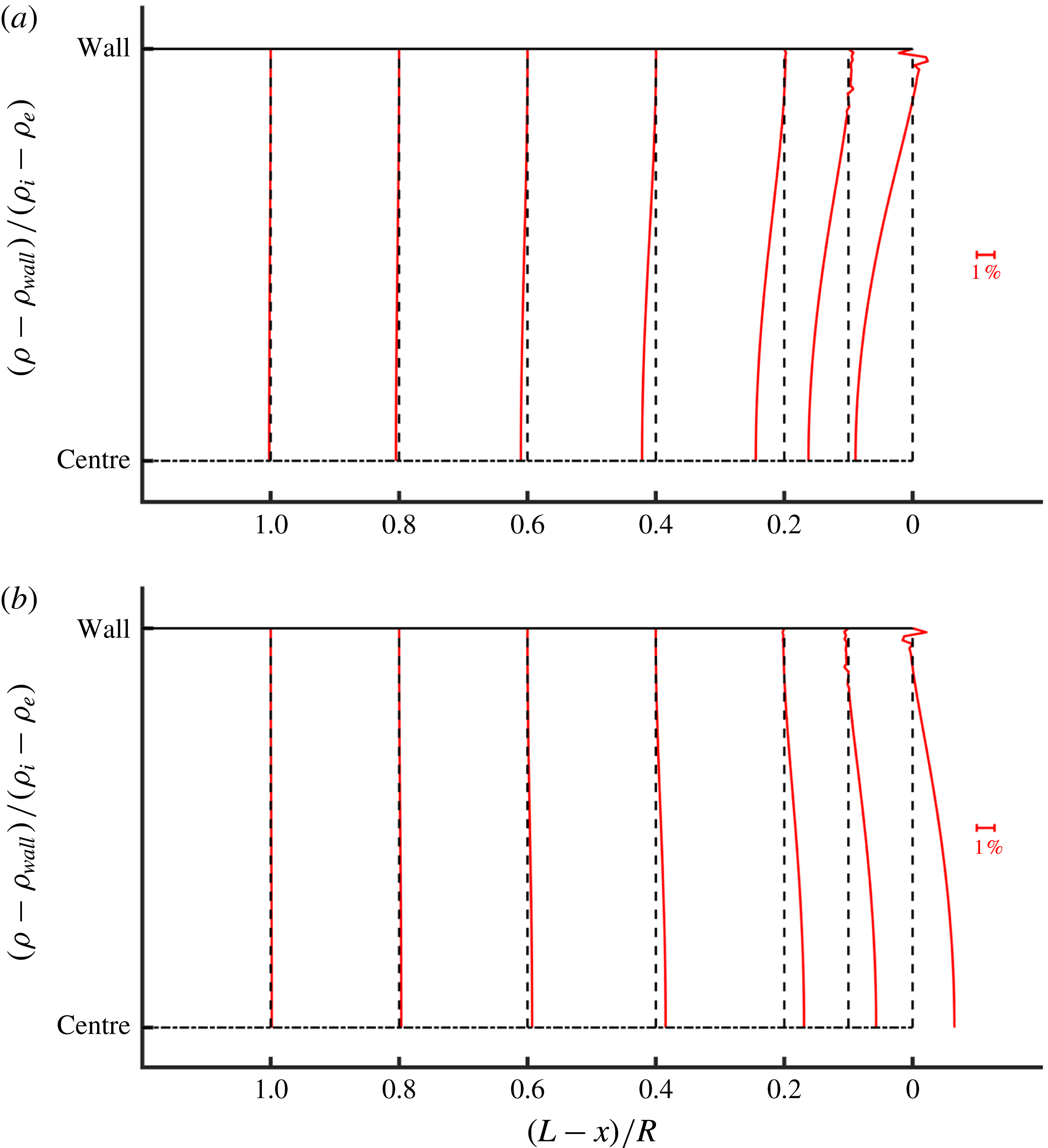
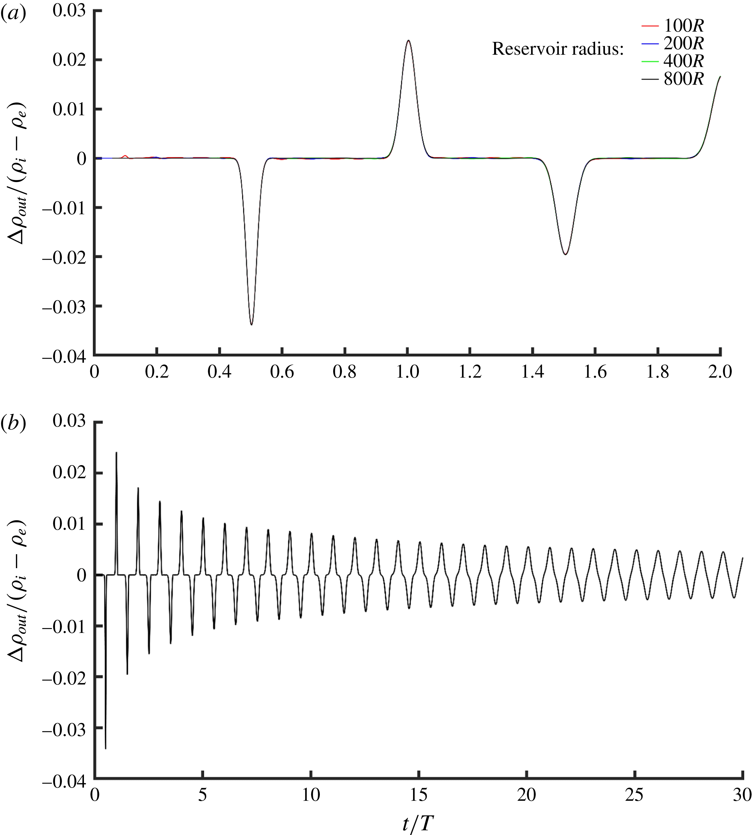
As expected, upstream from the tube exit, density is uniform over the tube cross-section (figure 5). As the fluid moves towards the tube exit, the density becomes non-uniform in the cross-section, indicative of the exit effect. At the tube exit, the maximum deviation of the density from $\unicode[STIX]{x1D70C}_{e}$ is defined as $\unicode[STIX]{x0394}\unicode[STIX]{x1D70C}_{out}$ , which changes with time and it can be positive or negative due to oscillation. This maximum density deviation is normalized against $\unicode[STIX]{x1D70C}_{i}-\unicode[STIX]{x1D70C}_{e}$ and plotted against the normalized time $t/T$ for various sizes of the reservoir in figure 6. Figure 6 shows that the maximum density deviation at the tube exit becomes independent of the reservoir size when the reservoir radius is greater than $100R$ . 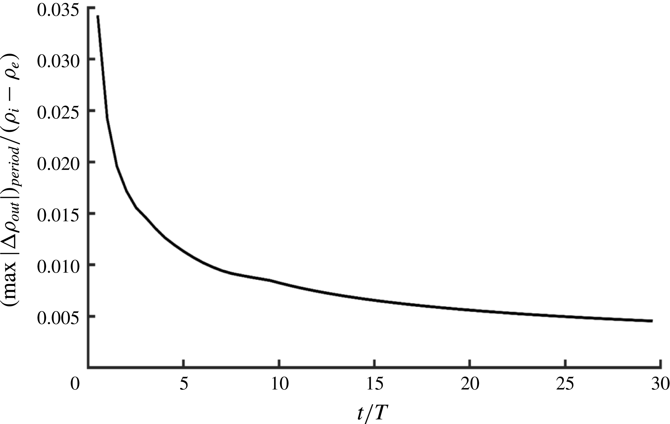In addition, the maximum density deviation decreases with time. The maximum of the absolute value of $\unicode[STIX]{x0394}\unicode[STIX]{x1D70C}_{out}$ in each period normalized with $\unicode[STIX]{x1D70C}_{i}-\unicode[STIX]{x1D70C}_{e}$ , $(\max |\unicode[STIX]{x0394}\unicode[STIX]{x1D70C}_{out}|)_{Period}/(\unicode[STIX]{x1D70C}_{i}-\unicode[STIX]{x1D70C}_{e})$ , is a measure of the maximum relative error in approximating the tube exit density as $\unicode[STIX]{x1D70C}_{e}$ (or, approximating $\unicode[STIX]{x1D70C}^{\prime }$ as zero at the tube exit). This maximum relative error is plotted against $t/T$ for a reservoir with a radius of $300R$ in figure 7. Clearly, this maximum error decreases quickly from approximately 3.5 % in the early times to just 0.5 % after about 25 periods. Since our interest is for large exit reservoir (compared to the narrow tube) and drainage rate at times much larger than the oscillation period, $t\gg T$ , ignoring the exit reservoir and approximating the density at the tube exit as $\unicode[STIX]{x1D70C}_{e}$ is justified. Furthermore, figure 5 indicates that the exit length is also small, about one tube radius for the case considered.

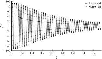
Numerical solutions are also carried out for a tube with a prescribed density $\unicode[STIX]{x1D70C}_{e}$ at the tube exit in the absence of an exit reservoir. Figure 8 compares the numerically computed normalized instantaneous mass flow rate at the exit $\tilde{{\dot{m}}}_{e}={\dot{m}}_{e}L^{2}/M_{L}D_{\unicode[STIX]{x1D70C}}$ with that from the analytical solution (5.1) against the dimensionless time on the diffusive time scale, $\bar{t}=D_{\unicode[STIX]{x1D70C}}t/L^{2}$ . Excellent agreements between the analytical solution and the numerical computation are achieved.

Figure 5.

Normalized local density difference $(\unicode[STIX]{x1D70C}-\unicode[STIX]{x1D70C}_{wall})/(\unicode[STIX]{x1D70C}_{i}-\unicode[STIX]{x1D70C}_{e})$ at various tube cross-sections upstream from the tube exit (solid lines). The dashed lines are for $\unicode[STIX]{x1D70C}-\unicode[STIX]{x1D70C}_{wall}=0$ and the scale bar is the percentage deviation from the dashed lines. ‘Centre’ and ‘Wall’ refer to the centreline and the wall of the tube. (a) At one half-period; (b) at one period.

Figure 6.

(a) Normalized density deviation $\unicode[STIX]{x0394}\unicode[STIX]{x1D70C}_{out}/(\unicode[STIX]{x1D70C}_{i}-\unicode[STIX]{x1D70C}_{e})$ at the tube exit as a function of time for various large reservoirs. These curves essentially coincide with each other when the reservoir has a radius greater than $100R$ . (b) Normalized density deviation for a reservoir with a radius of $300R$ covering a wider range of times.

Figure 7.

Maximum relative error $(\max |\unicode[STIX]{x0394}\unicode[STIX]{x1D70C}_{out}|)_{Period}/(\unicode[STIX]{x1D70C}_{i}-\unicode[STIX]{x1D70C}_{e})$ in approximating the tube exit density as $\unicode[STIX]{x1D70C}_{e}$ as a function of time.

Figure 8.

Comparison of dimensionless instantaneous mass flow rates between numerical solution and analytical solution. There is no exit reservoir and the exit density is fixed. The dimensionless time $\bar{t}=D_{\unicode[STIX]{x1D70C}}t/L^{2}$ is measured in terms of the long time diffusive time scale.

7 Diffusion equation and capillary with an absorbing end

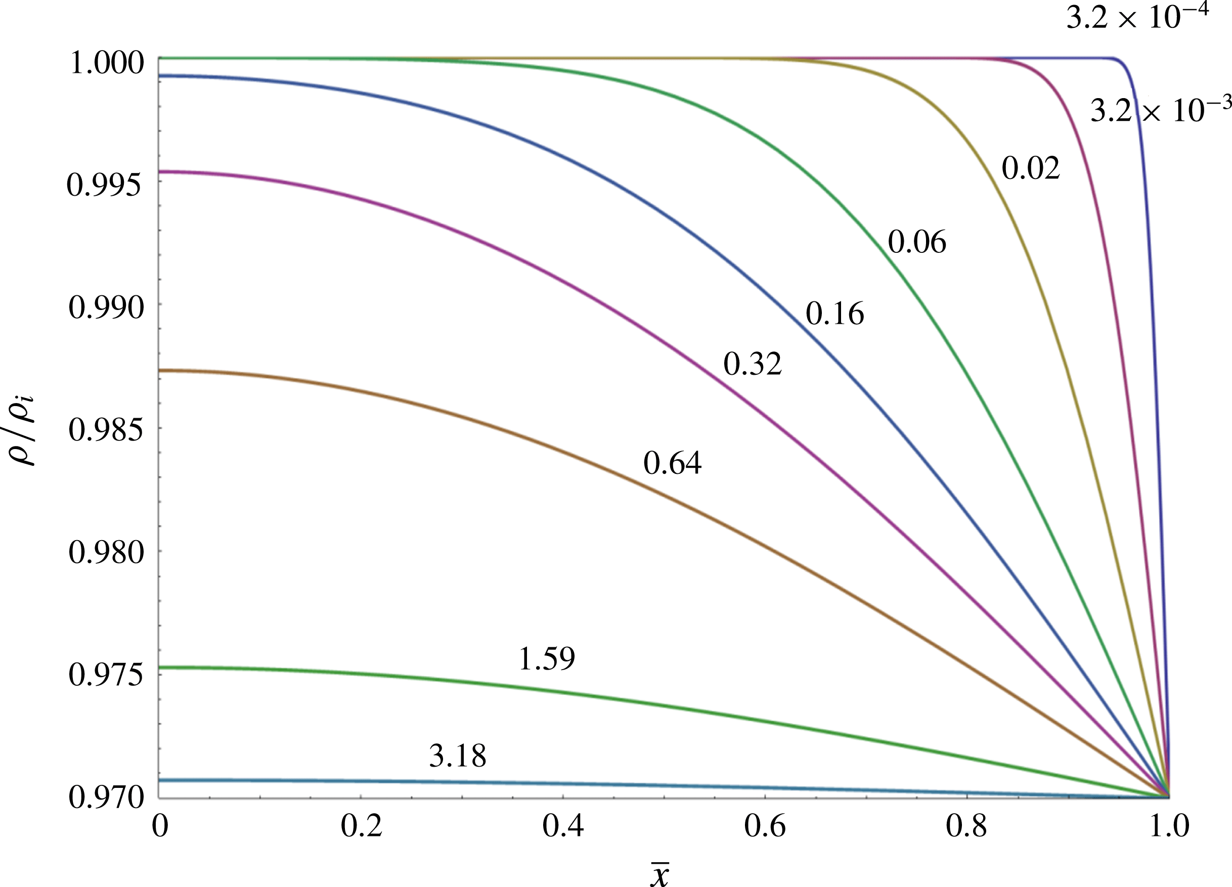
The envelope of the density oscillation (3.12) is diffusive,

The density envelope is plotted in figure 9, with the dimensionless time $\bar{t}=D_{\unicode[STIX]{x1D70C}}t/L^{2}$ . This envelope solution corresponds to the density change on the large diffusive time scale $L^{2}/D_{\unicode[STIX]{x1D70C}}$ when the fast oscillation in density has been smoothed out by integrating over the oscillation period.

Figure 9.

Diffusive decay of the density envelope. $D_{\unicode[STIX]{x1D70C}}=4.82\,\times \,$ $10^{-5}~\text{m}^{2}~\text{s}^{-1}$ . The numbers above each curve show the dimensionless time $\bar{t}$ .

The solution discussed so far assumes that the surface of the sealed end at $x=0$ is a perfect reflecting surface for sound waves, with the reflection coefficient $\Re =1$ . If, on the other hand, the surface of the sealed end is non-reflecting, $\Re =0$ , then the rarefaction wave will not be reflected by the sealed end at all. Thus, there will be no standing acoustic wave sloshing around inside the tube. The longitudinal propagation of the density perturbation is then controlled by pure diffusion shortly after the sound wave has reached the end of the tube. In other words, the damped wave equation for the density perturbation degenerates to the corresponding diffusion equation after a very short time,

The corresponding relaxed density solution is then (Carslaw & Jaeger Reference Carslaw and Jaeger1959)

The drainage rate becomes

Compared to the case of a reflecting sealed end equation (5.3), the drainage rate is twice as large but the exponents of exponential rate of decay are also twice as large. Thus, fluid is drained from the tube at a faster rate. This is due to the fact that the density in the tube approaches the equilibrium density much faster, as there is no wave motion to help maintaining the density perturbation in the tube. The drainage rates (5.3) and (7.4) both satisfy the condition $\int _{0}^{\infty }\hat{{\dot{m}}}_{e}(t)\,\text{d}t=M_{L}$ . It is thus observed that even though the drainage rate is controlled by the diffusion of the density perturbation, ignoring the existence of the acoustic wave and using the purely diffusive equation (7.2) from the outset for the case of a perfect reflecting end will lead incorrectly to the drainage rate (7.4) instead of (5.3). When there is a standing acoustic wave inside the capillary, fluid drainage is controlled by the decay of the wave amplitude, or the envelope of the wave. The density envelope equation is not the same as the diffusion equation (6.2); and it can be derived from the damped wave equation (2.3) by the method of multiple scales (Bender & Orszag Reference Bender and Orszag1978). The fast time scale is associated with the acoustic wave, $t_{F}=L/c$ , and the slow time scale is associated with diffusion, $t_{S}=L^{2}/D_{\unicode[STIX]{x1D70C}}$ , with the ratio $\unicode[STIX]{x1D700}=t_{F}/t_{S}=D_{\unicode[STIX]{x1D70C}}/cL\ll 1$ . Thus, the dimensionless damped wave equation using the fast time scale becomes

where $\bar{\unicode[STIX]{x1D70C}}=\unicode[STIX]{x1D70C}^{\prime }/\unicode[STIX]{x1D70C}_{e}$ , $\bar{t}=t/t_{F}$ . Introducing a slow time variable $\bar{\unicode[STIX]{x1D70F}}=\unicode[STIX]{x1D700}\bar{t}$ and expanding $\bar{\unicode[STIX]{x1D70C}}$ ,

leads to the equations at the following orders:

The leading-order equation is a wave equation which admits wave solution of the form $\bar{\unicode[STIX]{x1D70C}}_{0}=\bar{H}(\boldsymbol{x},\bar{\unicode[STIX]{x1D70F}})\exp (-\text{i}\unicode[STIX]{x1D714}\bar{t})$ with $\bar{H}(\boldsymbol{x},\bar{\unicode[STIX]{x1D70F}})$ being the envelope. To avoid secular growth for $\bar{\unicode[STIX]{x1D70C}}_{1}$ , the forcing term in (7.8) must vanish, leading to the envelope equation

which when restored to dimensional form becomes

Thus, the density envelope diffuses with a diffusion coefficient $D_{\unicode[STIX]{x1D70C}}/2$ , not $D_{\unicode[STIX]{x1D70C}}$ . This confirms the density envelope solution (7.1) and it explains the origin of the discrepancy between the drainage rates from the damped wave equation $\hat{{\dot{m}}}_{e}(t)$ and the purely diffusive equation $\hat{{\dot{m}}}_{e,diff}(t)$ , with the latter being incorrect when the sealed end is sound reflecting. This analysis also shows that the presence of the acoustic wave retards the diffusion of the density disturbance by reducing the diffusion coefficient by one half. The effect of this retardation is the doubling of the drain-out time from that of the purely diffusive process.

An absorbing surface has a reflection coefficient in the range $0<\Re <1$ . Thus, the two cases discussed so far can be considered as corresponding to the slowest drainage (perfect reflecting) and the fastest drainage (purely diffusive), respectively. In general, we expect the density perturbation to be similar to (3.12), but with spatially decaying amplitudes. This situation is complicated as the reflection coefficient $\Re$ is generally frequency dependent. However, if the reflection coefficient can be approximated as independent of frequency and we are not interested in the details of the wave motion, we can then simply model the drainage rate for a capillary with an absorbing end as

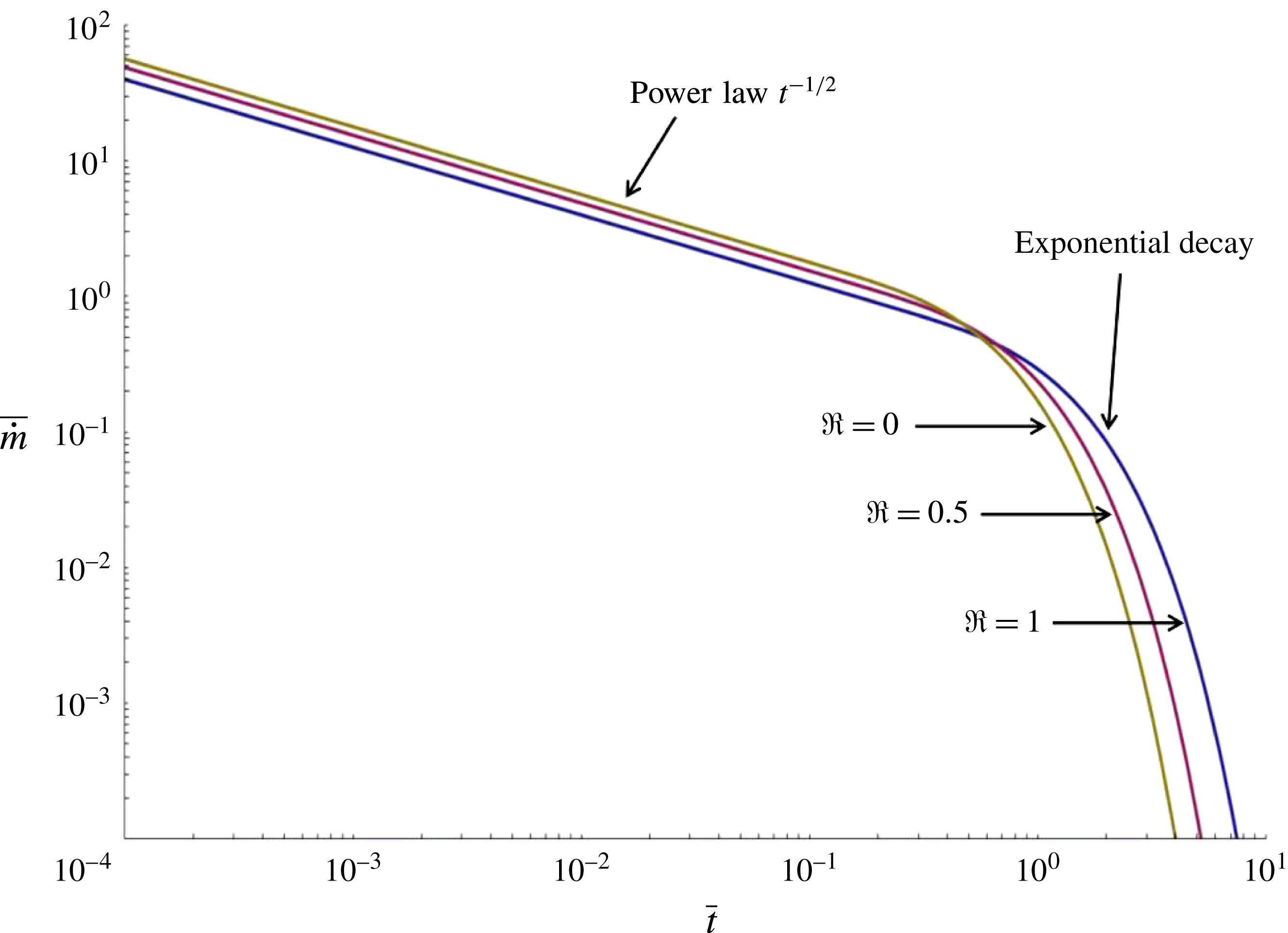
Dimensionless drainage rate $\bar{{\dot{m}}}_{e}$ and dimensionless drainage speed $\bar{V}_{e}(t)$ can be defined as

where the dimensionless time $\bar{t}=D_{\unicode[STIX]{x1D70C}}t/L^{2}$ . Figure 10 shows the dimensionless drainage rate $\bar{{\dot{m}}}_{e}$ (which is independent of radius) versus the dimensionless time $\bar{t}$ for various values of $\Re$ . The areas underneath these curves are all unity, reflecting the fact that the same amount of fluid is drained. The non-reflecting end ( $\Re =0$ ) has the highest drainage rate and the shortest drain-out time.

Figure 10.

Dimensionless drainage rate versus dimensionless time for various values of the reflection coefficient.