2. POSITION DETERMINATION BASED ON ODOMETRY

To calculate more accurate position and orientation, two positioning systems are utilised. The first and most basic positioning system is odometry and the second positioning system uses information from an Inertial Measurement Unit (IMU).

The robot's position is defined by $\underline{P}\lpar kT_{s}\rpar = \lsqb \underline{p}\lpar kT_{s}\rpar \comma \; \psi\lpar kT_{s}\rpar \rsqb ^{T}$ at time step kT _s ; where k is a positive integer and T _s is the sampling period. For simplicity T _s is dropped from the notation after this point and the mobile robot is assumed to be traveling on a flat surface. The vector $\underline{p}\lpar k\rpar = \lsqb p_{x}\lpar k\rpar \comma \; p_{y}\lpar k\rpar \rsqb ^{T}$ specifies the robot's Cartesian position, and ψ(k) defines the robot orientation. The kinematic model of the mobile robot is given by:

(1) $$\left\{ {\matrix{ {p_x(k + 1) = p_x(k) + {\rm }\left( {\displaystyle{{v_r(k) + v_l(k)} \over 2}} \right)T_s\cos \left( {\psi (k)} \right)} \hfill \cr {p_y(k + 1) = p_y(k) + {\rm }\left( {\displaystyle{{v_r(k) + v_l(k)} \over 2}} \right)T_s\sin \left( {\psi (k)} \right)} \hfill \cr {\psi (k + 1) = \psi (k) + {\rm }\left( {\displaystyle{{v_r(k) - v_l(k)} \over b}} \right)T_s} \hfill \cr } } \right.$$

where v _r and v _l are the robot right and left wheel velocities, respectively. ψ(k) is the angle between the robot direction and the X-axis, and b is the distance between the two wheels.

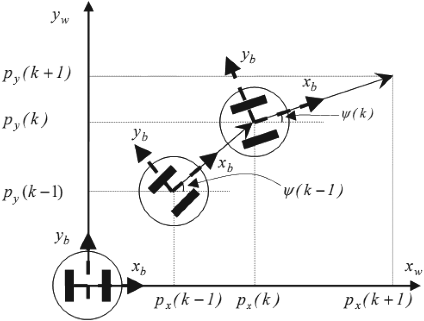
To characterise the mobile robot's motion, two coordinate frames are defined. The body coordinate frame (x _b , y _b ), as shown in Figure 1, is selected so that x is forward and y is lateral with the origin located at the robot's kinematics centre. The world coordinate frame (x _w , y _w ), is stationary and attached to the initial position of the robot. Initially, the body coordinate frame coincides with the world coordinate frame. As shown in Figure 1, the position vector $\underline{P}\lpar k\rpar $ is updated during the mobile robot motion with respect to the world coordinate frame.

Figure 1.

Mobile Robot position with respect to the World Coordinate Frame.

The robot position vector based on odometry is estimated incrementally by:

(2) $$\eqalign{& ^o \underline{p} (k + 1) = ^o\underline{p} (k) + R_{\psi _o}(k){\underline{v} }^b(k) \cr & \psi _o(k + 1){\rm } = \psi _o(k) + {\dot \psi }_o(k)T_s} $$

where $v^{b}\lpar k\rpar = \lsqb v^{b}_{x} \lpar k\rpar \comma \; v^{b}_{y} \lpar k\rpar \rsqb ^{T}$ , is the robot velocity in the body coordinate frame, $R_{\psi_{o}}\lpar k\rpar $ denotes the rotational transformation matrix from the body coordinate frame to the world coordinate frame and ψ _o (k) and $\dot{\psi}_{o}\lpar k\rpar $ , are the robot orientation and its angular velocity. $R_{\psi_{o}}\lpar k\rpar $ is specified by:

(3) $$R_{\psi _o}(k) = \left[ {\matrix{ {\cos \psi _o(k)} & { - \sin \psi _o(k)} \cr {\sin \psi _o(k)} & {\cos \psi _o(k)} \cr } } \right]$$

The velocity component $v^{b}_{y}\lpar k\rpar $ is assumed to be zero because of the robot's forward motion. $v^{b}_{x}\lpar k\rpar $ and ${\psi_{\circ}}\lpar k\rpar $ are calculated by:

(4) $$\eqalign{& {v_x^b} (k) = \displaystyle{1 \over 2}(v_{er}(k) + v_{el}(k)) \cr & {{\dot \psi }_{^\circ}} (k) = \displaystyle{{v_{er}(k) - v_{el}(k)} \over b}} $$

where v _er (k) and v _el (k) are the robot's right and left wheels' translational velocities, respectively. v _er (k) and v _el (k) are known from reading the encoder values and b is the robot wheelbase.

3. EQUATIONS OF THE INERTIAL NAVIGATION SYSTEM

In any INS, inertial sensors (accelerometers and gyroscopes) have been used to measure accelerations and angular velocity of a vehicle in relation to the inertial space. An Inertial Measurement Unit (IMU) is used to measure all accelerometers and gyroscopes of a system. The output information of the IMU enters the inertial processing unit in which inertial calculations of position, attitude and velocity of the system are performed at each moment in relation to the reference system, which is the Earth's coordinates, in the current work. In the coordinates of the Earth, the navigation operation is conducted as follows:

1. I. Position in a navigation system is calculated as:

   (5) $$\left\{ {\matrix{ {\dot L = \displaystyle{{v_N} \over {R_0 + h}}} \hfill \cr {\dot l = \displaystyle{{v_E} \over {{\rm (}R_0 + h{\rm )}\cos L}}} \hfill \cr {\dot h = - v_D} \hfill \cr } } \right.$$

where L, l and h are coordinates of a vehicle, and stand for Earth coordinates latitude, longitude and altitude of the vehicle, respectively. Moreover, $v_N,\;v_E\;and\;v_D$ indicate the velocity of the vehicle in the North, East and Down directions toward the centre of the Earth. R ₀ is the radius of the Earth, assumed as 6,378,140 metres.

1. II. To determine the attitude of the vehicle, the following equation is used.

   (6) $$\dot{C}^e_b = {C}^e_b \lpar \Omega^b_{ib} - {C}^e_b\Omega^e_{ie}\rpar $$

In the above equation, $\Omega^{b}_{ib}$ and $\Omega^{e}_{ie}$ are the anti-symmetric output vector of the gyroscope with the angular velocity of the Earth, and $C^{e}_{b}$ is the Direction Cosine Matrix (DCM) that converts the vector from coordinates of the navigation system into Earth coordinates. The anti-asymmetric matrix is also defined as follows:

(7) $$x = \left[ {\matrix{ {x_1} & {x_2} & {x_3} \cr } } \right]^T \Rightarrow X = \left[ {\matrix{ 0 & { - x_3} & {x_2} \cr {x_3} & 0 & { - x_1} \cr { - x_2} & {x_1} & 0 \cr } } \right]$$

1. III. The velocity of the vehicle is determined using the following equations:

   (8) $$\matrix{ {{\rm }\left\{ {\matrix{ {{\dot v}_N = f_N - v_E(2\Omega + \dot l)\sin L + v_D\dot L + \xi g} \hfill \cr {\quad {\mkern 1mu} \; = f_N - 2\Omega v_E\sin L + \displaystyle{{v_Dv_N - v_E^2 \tan L} \over {R_0 + h}} + \xi g} \hfill \cr {{\dot v}_E = f_E - v_N(2\Omega + \dot l)\sin L + \mathop {v_D}\limits^. (2\Omega + \dot l)\cos L - \eta g} \hfill \cr {\quad {\mkern 1mu} \; = f_E + 2\Omega (v_N\sin L + v_D\cos L) + \displaystyle{{v_E} \over {R_0 + h}}(v_D + v_N\tan L) - \eta g} \hfill \cr {{\dot v}_D = f_D - v_E(2\Omega + \dot l)\cos L - v_N\dot L + g} \hfill \cr {\quad {\mkern 1mu} \; = f_D - 2\Omega v_E\cos L - \displaystyle{{v_E^2 + v_N^2 } \over {R_0 + h}} + g} \hfill \cr } } \right.} \hfill \cr } $$

where $f_{N}\comma \; f_{E}\;{and}\ f_{D}$ are the acceleration of the vehicle in the North, East, and Down directions within the navigation system, respectively. They can be calculated from the following equation:

(9) $$\matrix{ {f^n} \hfill & { = C_b^n f^{b}} \hfill \cr {f^n} \hfill & { = [f_N\quad f_E\quad f_D]} \hfill \cr } $$

where f ^b is the calculated vector of the output of the accelerometers and $C^{n}_{b}$ is the DCM that is used for carrying the calculated quantities of accelerometers used in the body navigation system into the reference navigation system. In Equation (8), g _l is the local gravity vector of the Earth that can be estimated as follows if the elliptical effect of the Earth is neglected:

(10) $$g_l = \left[ {\matrix{ {\xi g} & {\eta g} & g \cr } } \right]^T = \left[ {\matrix{ 0 & 0 & {9\cdot 791719} \cr } } \right]^T$$

4. CUBATURE KALMAN FILTER ALGORITHM

All known filters suffer from problems such as divergence and the “curse of dimensionality”. The result of the “curse of dimensionality” is widely seen in state-space models with more than 20 states in the state vector. In other words, as the dimension increases the sample size must increase exponentially to keep a predefined level of accuracy for a given estimator. Here, divergence is due to different reasons such as:

• • The incorrectness or the deficiency of the available physical model of the system.

• • The inaccuracy or the unreliability of the information in measuring the function of density distribution.

• • The high dimension of nonlinear equations that simulate the state-space.

• • The computational and quantitative errors.

The CKF has been recently introduced to solve the problems of high dimensions and divergence that exist in previous version of KFs. This filter is a nonlinear filter that is established to estimate high dimension states based on spherical-radial rules. The cubic rules have no need to be differentiated; therefore, this algorithm can be used for those functions that are inherently difficult to be differentiated or their Hessian and Jacobian matrices cannot be computed.

The algorithm of the Cubature Kalman Filter includes the following steps:

1. 1) Suppose the primary density of the k − 1 moment has been calculated by the obtained data until the (k − 1)th moment. This density can be analysed as follows:

   (11) $$P_{k-1 \vert k-1} = S_{k-1 \vert k-1}S^{T}{_{k-1 \vert k-1}}$$
   where $S=\sqrt{P}$ and $\lpar \sqrt{P}\rpar _{i}$ denotes the ith row or column of the square root matrix P. If P = S ^T S, then i is the row number of S, and if P = SS ^T , then i is the column number of S. Furthermore, to find $\lpar \sqrt{P}\rpar _{i}$ , one can use the Cholesky factorisation method. However, the Singular Value Decomposition (SVD) method, which is simpler and more precise, is suggested.

2. 2) The cubic points are calculated as follows:

   (12) $$\chi_{i,k-1 \vert k-1} = S_{k-1 \vert k-1}\xi_{i} + \hat{x}_{k-1 \vert k-1}\quad i=1,2, \ldots ,m$$
   where m = 2n, n is the number of the states, and ξ _i denotes the i-th member of the below set, called the set of cubature points (Zarei and Shokri, Reference Zarei and Shokri2015):
   $$\sqrt {\displaystyle{m \over 2}} \left\{ {\left( {\matrix{ 1 \cr 0 \cr \cdot \cr \cdot \cr \cdot \cr 0 \cr } } \right),\left( {\matrix{ 0 \cr 1 \cr \cdot \cr \cdot \cr \cdot \cr 0 \cr } } \right),\left( {\matrix{ 0 \cr \cdot \cr \cdot \cr \cdot \cr \cdot \cr 1 \cr } } \right), \ldots ,\left( {\matrix{ { - 1} \cr 0 \cr \cdot \cr \cdot \cr \cdot \cr 0 \cr } } \right),\left( {\matrix{ 0 \cr { - 1} \cr \cdot \cr \cdot \cr \cdot \cr 0 \cr } } \right), \ldots ,\left( {\matrix{ 0 \cr 0 \cr \cdot \cr \cdot \cr \cdot \cr { - 1} \cr } } \right)} \right\}$$

3. 3) In this step, the cubic points are passed through the process equation, which represents the system dynamic:

   (13) $$\chi^{\ast}_{i,k \vert k-1}= F(\chi_{i-k-1 \vert k-1, u_{k-1}})$$

4. 4) By using the calculated points and by applying weights of the cubic points, the primary estimation is calculated as follows in the time update stage:

   (14) $$\hat x_{k \vert k - 1} = \displaystyle{1 \over m}\sum\limits_{i = 1}^m {\chi _{i,k \vert k - 1}^ * } $$

5. 5) The covariance matrix is calculated as follows in the time update stage:

   (15) $$P_{k \vert k - 1} = \displaystyle{1 \over m}\sum\limits_{i = 1}^m {\chi _{i,k \vert k - 1}^* } \chi _{i,k \vert k - 1}^{*T} - \hat x_{k \vert k - 1}\hat x_{k \vert k - 1}^T + Q_{k - 1}$$

6. 6) In this step, the computed matrix in step (5) is re-analysed as follows to compute new cubic points:

   (16) $$\eqalign{& P_{k \vert k - 1} = S_{k \vert k - 1}S^T_{k \vert k - 1} \cr & \chi _{i,k \vert k - 1} = S_{k \vert k - 1}\xi _i + {\hat x}_{k \vert k - 1}} $$

7. 7) In this step, the computed points must be passed through the measuring model:

   (17) $$\eqalign{ Y_{i,k \vert k-1}= H(\chi_{i,k \vert k-1}, u_{k})}$$

8. 8) By considering the calculated points and by applying the weights of the cubic points, the output of the system is estimated as follows:

   (18) $$\matrix{ {{\hat y}_{k \vert k - 1} = \displaystyle{1 \over m}\sum\limits_{i = 1}^m {y_{i,k \vert k - 1}} } \hfill \cr } $$

9. 9) In this step, the covariance matrices associated with the output and intersecting with the input-output of the system are computed to calculate the gain of the KF.

   (19) $$\matrix{ {P_{yy,k \vert k - 1} = \displaystyle{1 \over m}\sum\limits_{i = 1}^m {Y_{i,k \vert k - 1}} - {\hat y}_{k \vert k - 1}\hat y_{k \vert k - 1}^T + R_k} \hfill \cr {P_{xy,k \vert k - 1} = \displaystyle{1 \over m}\sum\limits_{i = 1}^m {X_{i,k \vert k - 1}} - {\hat x}_{k \vert k - 1}\hat y_{k \vert k - 1}^T } \hfill \cr } $$

10. 10) Compute the gain of the KF as follows:

    (20) $$\matrix{ {W_k = P_{xy,k \vert k - 1}P_{yy,k - 1}^{ - 1} } \hfill \cr } $$

11. 11) In the measurement update stage, the new estimation is computed by utilising a new measurement as follows:

    (21) $$\matrix{ {{\hat x}_{k \vert k} = {\hat x}_{k \vert k - 1} + W_k(y_k - {\hat y}_{k \vert k - 1})} \hfill \cr } $$

12. 12) Updating the covariance matrix:

    (22) $$\matrix{ {P_{K \vert K} = P_{k \vert k - 1} - W_kP_{yy,k \vert k - 1}W_k^T } \hfill \cr } $$

13. 13) To compute the next updated estimated state, steps 1 to 12 should be repeated.

5. INTEGRATING THE INERTIAL NAVIGATION SYSTEM WITH THE ODOMETRY

In the previous research, the EKF is used to determine the robot's position and orientation by integrating information from multiple sensors (Borenstein and Feng, Reference Borenstein and Feng.1995; Reference Borenstein and Feng1996a; Reference Borenstein and Feng1996b). The EKF was developed to extend the application of the Kalman filter to nonlinearity issues. The CKF achieves better performance than the EKF in dealing with nonlinear problems (Jwo et al., Reference Jwo, Hu and Tseng2013; Wendel et al., Reference Wendel, Meister, Schlaile and Trommer2006; Zhao and Slotine, Reference Zhao and Slotine2005). This paper demonstrates the applicability of using the CKF for a more accurate mobile robot position determination.

5.1. Data fusion by using the extended Kalman filter

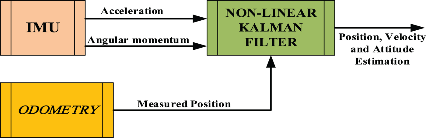
Figure 2 shows the block diagram of data fusion by using extended Kalman filters. As shown in this figure, the difference between the estimated position from INS and the measured position from the odometry are considered as the computed input of the EKF.

(23) $$\matrix{ {y = \left[ {\matrix{ {\delta P_{INS,X} - \delta P_{odometry,X}} \cr {\delta P_{INS,Y} - \delta P_{odometry,Y}} \cr } } \right]} \hfill \cr } $$

Figure 2.

The Algorithm of Integrating INS/ODOMETRY by EKF.

The process equation is considered as:

(24) $$ \eqalign{{\delta x_k} \hfill & = {F(\delta x_{k - 1},u_{k - 1})} \hfill \cr {\delta x} \hfill & = {{\left[ {\matrix{ {\delta L} & {\delta l} & {\delta V_n} & {\delta V_E} & {\phi _N} & {\phi _E} \cr } } \right]}^T} \cr {\bf u} \hfill & = {{\left[ {\matrix{ {\delta {\bf f}^B} & {\delta {\bf \omega }_{IB}^B } \cr } } \right]}^T}} $$

where δ x includes the vector of attitude error, the vector of velocity error and the vector of rotating attitude error. The input u includes the main sources of errors that are known as errors of accelerometers and gyroscopes.

Now, the EKF is exploited to estimate INS errors. By applying these errors, INS parameters will be updated to rectify errors and prevent instability of the system. It should be mentioned that these errors are calculated after data sampling.

5.2. Data fusion by using nonlinear Kalman filters

In Figure 3, the general structure of fusion algorithm for the navigation system using nonlinear Kalman filters is shown. It is clear from this figure that this structure consists of an auxiliary navigation system (i.e. odometry) and an estimation algorithm such as an unscented or cubature Kalman filter, which estimate the navigation states.

Figure 3.

The algorithm of integrating INS/ODOMETRY using a CKF.

In this structure, linear and angular acceleration and position of the body are measured at each step by using IMU and auxiliary navigation systems, respectively. Then, the state estimator (unscented or cubature Kalman filter) estimates the navigation system states (position, velocity and the situation of moving the body) without any error. The process state equation is expressed as follows:

(25) $$ \eqalign{ {x_k} \hfill & = {F(x_{k - 1},u_{k - 1})} \hfill \cr x \hfill & = {{\left[ {\matrix{ L & l & {V_n} & {V_E} & {\phi _N} & {\phi _E} \cr } } \right]}^T} \hfill \cr {\bf u} \hfill & = {{\left[ {\matrix{ {{\bf f}^B} & {{\bf \omega }_{IB}^B } \cr } } \right]}^T}} $$

where x denotes the position, velocity and rotational position vector. Input u includes the linear and angular velocities measured by the IMU. Also, the measurement equation for fusion by using nonlinear filters is expressed in Equation (26):

(26) $$y = \left[ {\matrix{ {P_{odometry,X}} \cr {P_{odometry,Y}} \cr } } \right]$$

The proposed data fusion approach in this section is not only simple to implement, but can also reduce the computational complexity and improve the accuracy of the localisation. Moreover, the main advantage of using this method is that correction can be completed using at least one available measurement signal (y) or IMU. The more measurement signals become available, the more accurate the estimation will be.

6. SIMULATION RESULTS

In this section, the suggested algorithm has been analysed based on a set of simulated data that was obtained from a robot movement over 600 seconds. The goal in this simulation is to examine the applicability of the proposed approach for short and long runs.

The gyroscopes and accelerometers' scaling factor error and biases are considered as follows:

(27) $$\eqalign{S_g &= diag\left[ {\matrix{ {{10}^{ - 2}} & {{10}^{ - 2}} & {{10}^{ - 2}} \cr } } \right]\quad ({\rm deg}/h) \cr S_a &= diag\left[ {\matrix{ {{10}^{ - 2}} & {{10}^{ - 2}} & {{10}^{ - 2}} \cr } } \right]\quad \,(m/s^2) \cr \varepsilon _{const}^B &= \left[ {\matrix{ {0\cdot 2} & {0\cdot 2} & {0\cdot 2} \cr } } \right]\quad \,\,\,\,\,\,\,\,\,\,\,\,\,\,\,\,\,\,({\rm deg}/h) \cr \eta _{const}^B &= \left[ {\matrix{ {{10}^{ - 4}g_0} & {{10}^{ - 4}g_0} & {{10}^{ - 4}g_0} \cr } } \right] \;(m/s^2)} $$

where S _g and S _a are 3 × 3 diagonal matrices whose principal diagonal elements are valued considering the gyroscopes and accelerometers' scaling factor error. Furthermore, $\varepsilon^{B}$ and η ^B are the gyroscopes and accelerometers' biases.

In addition, numerical values of measurement noise covariance R, process noise covariance Q, initial estimation of the states $\hat x_0$ and initial error of the covariance P ₀ for the nonlinear Kalman filters are considered as follows:

(28) $$\matrix{ R \hfill & { = [{10}^{ - 12}\quad {10}^{ - 12}]} \hfill \cr Q \hfill & { = diag[{10}^{ - 4}\quad {10}^{ - 4}\quad {10}^{ - 4}\quad {10}^{ - 4}\quad {10}^{ - 4}]} \hfill \cr {\hat x} \hfill & { = {[53\quad - 1\cdot 7\quad 0\quad 1\cdot 41\quad 0]}^T} \hfill \cr {P_0} \hfill & { = diag[{10}^{ - 3}\quad {10}^{ - 3}\quad {10}^{ - 2}\quad {10}^{ - 2}\quad {10}^{ - 1}]} \hfill \cr } $$

It is worth mentioning that roll and pitch angles are equal to zero due to the robot movement on the ground. Moreover, the downward acceleration in the vertical direction (centre of the Earth) will not be considered. Therefore, in this study, only the heading and angular velocity along the East and North directions are estimated.

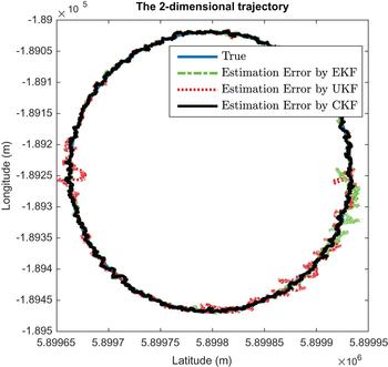
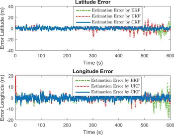
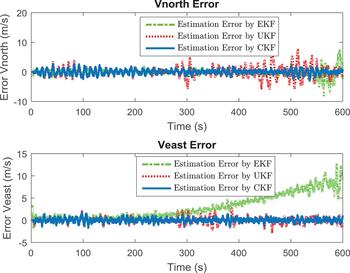
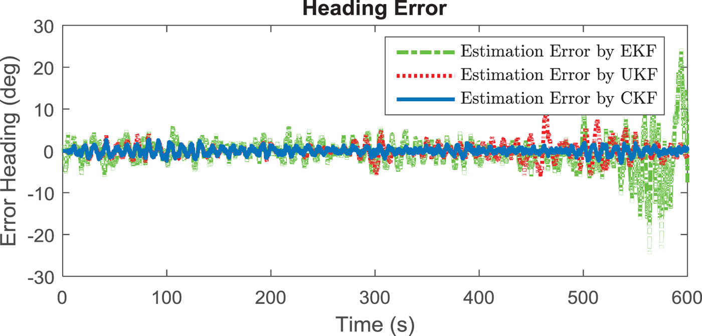
The robot's final position and orientation are recorded and the estimates of the robot's position along the North and East and the orientation based on the EKF, UKF, and CKF, using information from the INS, and odometry are compared with the actual trajectory. Width, length, and the velocity in North and East directions are calculated by the EKF, UKF and CKF algorithms and are compared with the real quantity of these parameters. The obtained results are shown in Figures 4 to 7.

Figure 4.

Two-dimensional trajectory of the robot.

Figure 5.

Latitude estimation error (above), longitude estimation error (below).

Figure 6.

Vnorth estimation error (above), Veast estimation error (below).

Figure 7.

Heading estimation error.

To analyse the reliability of the approach the experiment was repeated twenty times. The averages of final position and orientation errors for twenty runs are listed in Table 1. Based on the obtained results, it can be argued that the CKF provides position and orientation that are more precise than other positioning systems such as odometry, IMU and those corrected by the EKF.

Table 1.

RMSE of Position and Orientation Errors for Twenty Runs.