3.1 Phase-averaged vortex structure

The jet was positioned at a pressure node of the transverse acoustic mode in the rectangular box. Therefore, the incoming jet flow is not modified by acoustic pressure oscillations in the box, resulting in negligible levels of velocity oscillations in the inlet bulk flow velocity. However, this location is also an acoustic velocity anti-node location. Therefore, the application of acoustic forcing results in a strong transverse flapping motion of the jet at the forcing frequency, which can be viewed as the superposition of both $m=\pm 1$ azimuthal modes. While the acoustic transverse velocity oscillations were described previously in figure 2(d), to describe the inlet conditions in more detail the velocity profiles in the $x$ – $y$ plane close to exit are shown in figure 3.

The phase-averaged exit profiles show a strong dependence on phase angle as expected. Close to the jet axis ( $r/D=0$ ) the transverse component follows the acoustic velocity, switching sign sinusoidally. The strong peaks and troughs at the jet edges ( $r/D\approx \pm 0.5$ ) are associated with the induced velocity from the coherent vortex structures located in the shear layers (discussed below). Similar features related to the vortices can also be observed in the streamwise velocity profiles. The changing centres of the streamwise profiles additionally demonstrate the flapping motion of the jet, even at this small downstream distance.

In order to understand the structure and phase-averaged dynamics of the jet we begin by studying isosurfaces of normalised vorticity magnitude, $|\unicode[STIX]{x1D74E}^{\ast }|=|\unicode[STIX]{x1D74E}|D/u_{e}$ , at three points in the forcing cycle, as shown in figure 4. The isosurfaces have been coloured by the normalised transverse component of vorticity, $\unicode[STIX]{x1D714}_{y}^{\ast }=\unicode[STIX]{x1D714}_{y}D/u_{e}$ , in order to more clearly identify separate structures and to indicate the orientation of vorticity.

Figure 4.

Three-dimensional isosurfaces of normalised vorticity magnitude, $|\unicode[STIX]{x1D74E}^{\ast }|$ , at three points in the forcing cycle. A threshold level of $|\unicode[STIX]{x1D74E}^{\ast }|=6$ was chosen to highlight the vortex structure. The isosurfaces have been coloured by the normalised cross-stream component of vorticity, $\unicode[STIX]{x1D714}_{y}^{\ast }=\unicode[STIX]{x1D714}_{y}D/u_{e}$ , in order to more clearly identify separate structures and to identify the orientation of vorticity. Sine wave inset in upper left corner of each panel indicates the transverse velocity at each phase angle. Annotations identify: A, initial roll-up of the cylindrical vortex sheet shed from the nozzle lip; B1, formation of hairpin head; B2, formation of hairpin legs; C, the legs of the hairpin being drawn through the arch of the preceding structure; D, the formation of oscillations along the head; E, the increasing inclination angle of hairpin structures as they are advected downstream; F, the break-up of the head and reorientation of vortex lines with the legs of the following structure; G, the break-up of coherent structures at the end of the near field.

As the jet flaps in the transverse direction, vorticity generated in the shear layer is observed to roll up periodically, forming a train of large coherent vortex structures which are advected downstream. The topology of these structures can be described as inverted hairpins (or horseshoes), with the head and legs of each hairpin structure aligned in the cross-stream and transverse directions respectively. The head and legs of a single structure have been marked in figure 4 as B1 and B2, respectively. The term inverted here refers to the legs of each hairpin preceding the head in the streamwise direction. The structures are oriented in this manner at formation due to the inclination of the jet when the roll-up process begins. The orientation of the jet can be observed from the isosurfaces close to the jet exit ( $x/D=0$ ), showing the orientation of the cylindrical shear layer (marked in figure 4 as A). The orientation can also be inferred from the transverse velocity (shown previously in figure 2 d), which is identified in each panel through the sine wave inset in the upper left corner. It should also be noted that as roll-up occurs when the trajectory of the jet changes direction, two hairpin structures are formed on opposite sides of the jet during each forcing cycle. This behaviour is qualitatively different from that of a jet experiencing purely longitudinal oscillations, a process which results in the formation of a single vortex ring structure during each oscillation cycle (Aydemir et al. Reference Aydemir, Worth and Dawson2012). The rapid organisation of the coherent structures in anti-phase with respect to the $x$ – $z$ symmetry plane appears to be qualitatively similar to the alternating pairing structure observed by Urbin & Metais (Reference Urbin, Metais, Chollet, Voke and Leonhard1996) and da Silva & Métais (Reference da Silva and Métais2002), although in the present investigation this pairing occurs immediately downstream of the exit. This much more rapid organisation is therefore similar to the structures observed by Suzuki et al. (Reference Suzuki, Kasagi and Suzuki2004).

The transverse flapping motion of the jet also causes the hairpin heads to be located further from the jet centreline in comparison with the legs, resulting in lower advection velocities. This results in an increase in the inclination angle of the hairpin structures with downstream distance from the nozzle due to differences in these advection velocities (with this observation marked E in figure 4). These two observations are quantified in § 3.2. Furthermore, as each hairpin structure advects downstream, the velocity field induced by the head can be observed to draw the legs of the upstream structure through the arch of the hairpin (marked C in figure 4), drawing the two legs of each structure closer together. This process can also be seen to modify the local inclination of the structure. Once they have been threaded through the arches in this manner, the proximity of these leg vortex cores results in the breakdown of the hairpin head, which can then be observed to realign with the legs from the upstream structure (marked D and F in figure 4). As the structures advect further downstream ( $x/D\geqslant 2$ ) this unstable reconnection around the hairpin heads can be observed to result in rapid breakdown of the coherent structure (marked G in figure 4). The time-dependent formation and downstream evolution of the vortex structures can be more clearly understood from supplementary movies 1 and 2 of normalised vorticity magnitude.

Figure 5.

Slices of normalised vorticity, $\unicode[STIX]{x1D714}_{z}^{\ast }=\unicode[STIX]{x1D714}_{z}D/u_{e}$ , in the $x$ – $y$ plane, at $z/D=0$ , at six points in the forcing cycle. Velocity vectors at the jet exit are included to help identify the corresponding flapping motion of the jet (showing every third vector).

In order to further investigate the position of these vortex structures it is useful to study the components of the vorticity field in different planes of interest. Figure 5 shows the variation of the normalised cross-stream component of vorticity, $\unicode[STIX]{x1D714}_{z}^{\ast }=\unicode[STIX]{x1D714}_{z}D/u_{e}$ , on the $x$ – $y$ plane along the axis of the jet at $z/D=0$ , at six instants in the oscillation cycle. This plane of interest therefore cuts through the heads of the inverted hairpin structures, and shows a train of vortex cores of opposite-sign vorticity on the left- and right-hand side of the plot. Close to the exit, structures on the same side of the jet are separated by $\unicode[STIX]{x0394}x/D\approx 1$ which corresponds to their advection during a single oscillation cycle at the mean shear-layer velocity, $(u_{e}/2)/f_{f}D=1$ . However, the downstream location of the vortex cores is staggered between the right- and left-hand sides of the plot, with a difference in axial location of $\unicode[STIX]{x0394}x/D\approx 0.5$ . This is expected due to the transverse flapping of the jet in response to the acoustic forcing. The formation of structures on the left- and right-hand side of the jet occurs in anti-phase as illustrated by the position of the vortex cores. Close to the jet exit the transverse location of the vortex cores on both sides is $y/D\approx \pm 0.6$ , which increases slightly with downstream distance. It is also observed that the flapping of the jet results in an elongated roll-up process. As the jet changes direction the vortex core is located at a larger radial position in comparison with the remaining shear layer, which continues to therefore pass inside of the core. The remaining shear-layer vorticity continues to wrap around and even over the top of the existing vortex core, both increasing its circulation and additionally forming a smaller satellite core downstream. As downstream distance increases the core locations become less distinct as the vortex structure begins to break up, and complex merging and interactions between subsequent structures occur. It should be noted that there is some persistent asymmetry present between structures on the left-hand ( $y/D<0$ ) and right-hand ( $y/D>0$ ) sides of the domain. This is ascribed to the imperfect alignment of the jet with the acoustic node position in the enclosure.

Figure 6.

Sketch of the vortex sheet roll-up process in the $x$ – $y$ plane. The vector arrow at the bottom centre of each panel represents the jet velocity.

The roll-up mechanics is also shown in this plane, and can be described further through a sketch of the process in figure 6, which represents roll-up through the dynamics of the vortex sheet. At $t/T=0$ the magnitude of the transverse acoustic velocity is at a maximum in the negative $y$ direction. As the oscillation cycle progresses, the transverse acoustic velocity changes sign, and in response the jet flaps from its leftward inclined orientation at $t/T=0$ , first to slight leftward orientation at $t/T=1/6$ , and then to a slight rightward inclined orientation at $t/T=2/6$ . This flapping produces an inflection in the vortex sheet, indicated by point A in figure 6. The sign of the vorticity on the left-hand side is such that the fold in the sheet now begins to roll up under the action of induction, with point A indicating the rolled-up vortex core head location. During half the oscillation cycle, as the jet flaps from left to right a single hairpin structure is therefore formed. Despite a similar inflection formed through the flapping of the jet, the vortex sheet on the right-hand side of the jet remains stable during the first half of the cycle (shown through a point at a similar height, marked B in figure 6) due to the sign of the vorticity on this side. However, once the jet flaps from right to left to complete a single full oscillation cycle (from $t/T=3/6$ to $t/T=0$ ), a second structure is formed on the right-hand side of the jet, due to the now unstable arrangement of the vortex sheet. This roll-up process is therefore distinct from a jet experiencing longitudinal oscillations, in which a variation in circulation along the vortex sheet in the streamwise direction produces roll-up. The current constant circulation vortex sheet roll-up process is driven by the spatial rearrangement of the sheet, through the flapping action of the jet.

Figure 7 shows the variation of the normalised transverse component of vorticity, $\unicode[STIX]{x1D714}_{y}^{\ast }=\unicode[STIX]{x1D714}_{y}D/u_{e}$ , in the $x$ – $z$ plane, at six points in the oscillation cycle. The plane is positioned along the axis of the jet at $y/D=0$ , and therefore cuts through the legs of the hairpin structures. In this plane the shear layer is observed to form a train of vortical structures, with structures on either side of the jet centreline having opposite-sign vorticity. In contrast with the cross-stream plots (shown in figure 5), the vorticity distribution in the transverse plane is approximately symmetric. Structures at the same downstream location on the left- and right-hand side of the plot correspond to the left- and right-hand legs of a single hairpin structure, which is formed at the same point in the forcing cycle. Given that two hairpin structures are formed during each oscillation cycle, and that each pair of legs can be observed in this plane, the streamwise distance between vortex cores is $\unicode[STIX]{x0394}x/D\approx 0.5$ . It should also be noted that in comparison with the head locations, the cross-stream location of the vortex cores on both sides of the jet is $z/D\approx \pm 0.5$ close to the jet exit, and decreases slightly with downstream distance.

The symmetry observed in the $x$ – $z$ plane, and the anti-symmetry observed in the $x$ – $y$ plane together with the observations of the three-dimensional structure therefore demonstrate that the current application of transverse acoustic forcing results in the formation of plane-symmetric vortex structures about the $x$ – $z$ plane, which exist with a phase difference of half the forcing cycle. In other words the instantaneous structure of the jet is instantaneously anti-symmetric about the $x$ – $z$ plane, and plane-symmetric in the mean.

Figure 7.

Slices of normalised vorticity, $\unicode[STIX]{x1D714}_{y}^{\ast }=\unicode[STIX]{x1D714}_{y}D/u_{e}$ , in the $x$ – $z$ plane, at $y/D=0$ , at six points in the forcing cycle. Velocity vectors at the jet exit are included (showing every third vector).

3.2 Vortex tracking

In order to quantify the observation that the advection velocity of the hairpin head and legs is different, a simple vortex tracking algorithm was employed. Local vorticity maxima above a threshold value of $|\unicode[STIX]{x1D714}^{\ast }|>4$ were located in the jet centreline vorticity slices presented in figures 5 and 7, which allow the in-plane location of the vortex cores described as the hairpin heads and legs to be defined. This choice of slices captures one location for the vortex core of the head, and two locations for the corresponding vortex cores of the legs. A least squares fit to a two-dimensional Gaussian vorticity distribution was performed over a $7\times 7$ vector window around each of the local maxima in order to determine their locations to sub-vector spacing resolution. The vortex tracking algorithm was applied to each of the phase-averaged fields and the positions of the cores plotted with varying cycle time, as shown in figure 8(a). It should be noted that vortex cores formed during four oscillation cycles are simultaneously present in the measurement volume, and therefore the spatial locations of the vortex core positions have been unwrapped with respect to the oscillation cycle to aid the interpretation of their positions. Tracking results from the inviscid vortex model are also plotted in this section, but are discussed further in § 3.3.

Figure 8(a) shows the position of both the vortex core head and legs. Vortex cores associated with structures of opposite orientation are identified separately, with a distinction made between structures with heads lying on either the left-hand ( $y/D<0$ ) or right-hand ( $y/D>0$ ) sides of the jet, hereafter referred to as LHS and RHS structures. This separation was made in order to account for the phase difference between structures, allowing a $t/T=-1/2$ shift to be applied to RHS structures in order to collapse the data. Despite a small amount of positional scatter, structures on both sides of the jet share similar dynamics. The location of the hairpin head is observed to vary approximately linearly with time, therefore advecting at a near-constant rate. As expected from the inverted orientation of the hairpin structures shown previously, at a given instant in time the hairpin legs are downstream of the heads. Therefore, in figure 8(a) the scattered points denoting the hairpin leg locations are located above the head locations. The downstream location of each pair of hairpin legs is shown to match very closely, meaning that the hairpin structures are symmetric about the $x$ – $z$ plane. The location of the legs is also observed to vary approximately linearly with time, again corresponding to a near-uniform advection velocity. However, calculating a linear line of best fit to the core locations demonstrates through the differing slopes that the advection velocities of the head and legs differ, with mean advection velocities of $u_{head}/u_{e}=0.45$ and $u_{legs}/u_{e}=0.53$ calculated for the head and legs, respectively.

Figure 8.

Vortex core tracking results. In both panels the filled markers show structures with the heads on the left-hand side ( $y/D<0$ ) and open markers show structures with heads on the right-hand side ( $y/D>0$ ). (a) Non-dimensional vortex core location against time shows the different advection velocities of cores in the $x$ – $y$ plane (blue circles) and in the $x$ – $z$ plane (red squares and triangles). Solid and dashed lines represent the leg and head positions, respectively, calculated using the vortex model (VM). (b) Variation of the hairpin inclination angle, $\unicode[STIX]{x1D6F7}$ , with downstream distance. The solid line shows the ring angle calculated using the VM.

The difference in advection velocity between the head and legs of each hairpin means that as these structures advect downstream the difference in location between the head and legs increases (as shown by the diverging lines in figure 8 a), meaning the inclination angle of the structures also increases. An estimate of the hairpin inclination angle, $\unicode[STIX]{x1D6F7}$ , can be made by relating the downstream location of the head and legs at each point in the cycle according to $\unicode[STIX]{x1D6F7}=\arctan ((x_{head}-x_{legs})/|y_{head}|)$ . The variation of $\unicode[STIX]{x1D6F7}$ with time is shown in figure 8(b). The plot shows that immediately after the hairpin structure pinches off, it has an inclination of $\unicode[STIX]{x1D6F7}\approx 25^{\circ }$ . Based on the magnitude of the transverse acoustic velocity oscillations, the maximum jet angle at exit is approximately $6^{\circ }$ . Therefore during the roll-up process, the fluid entering the head and legs of each hairpin structure must also advect at differing velocities, increasing the inclination angle by another $19^{\circ }$ over three-quarters of a cycle. While the rate of this initial inclination increase is not possible to quantify, due to a lack of data at the jet exit, and the difficulty of defining the location of the structure prior to pinch-off, a similar difference in advection rates to the newly pinched-off structure would provide such an increase in inclination over this period. Following pinch-off, the inclination angle is shown to increase with downstream distance with the structure reaching an angle of $\unicode[STIX]{x1D6F7}\approx 40^{\circ }$ before breaking up.

The reduced advection velocity of the hairpin heads is due to their repositioning through the action of the jet flapping. This is quantified in figure 9, which shows the variation in radial location of the vortex cores with downstream distance. The markers show that the vortex cores are more widely spread in the $x$ – $y$ plane, with a mean position of $y/D\approx 0.6$ , compared with the position of the cores in the $x$ – $z$ plane, which are initially spaced at $z/D\approx 0.5$ . However, as shown previously in figure 2(a), even close to exit, the jet appears to be spreading more rapidly in the $y$ direction due to the transverse acoustic excitation. Therefore it is useful to analyse the location of the vortex cores together with the local spreading rate, defined as the jet half-width $y_{1/2}$ in the $x$ – $y$ plane, where $u(y)/u_{e}=1/2$ , or $z_{1/2}$ in the $x$ – $z$ plane, where $u(z)/u_{e}=1/2$ . In the current study to account for the imperfect alignment of the jet with the acoustic mode, we define the jet half-width separately for left- and right-hand sides on each plane of interest, allowing the vortex location to be compared to the local jet velocity in each case. While the vortices in the $x$ – $z$ plane closely follow the mean shear-layer velocity, the cores the $x$ – $y$ plane periodically fall above this line, and, as a consequence, are advected more slowly downstream. This periodic oscillation in radial location also results in the periodic oscillation in the hairpin inclination angle observed in figure 8(b). The jet spreading behaviour is also noteworthy, with a significantly enhanced spreading rate in the transverse direction beyond $x/D>2$ , although beyond this location there is considerable asymmetry in the spreading rate on left- and right-hand sides.

Figure 9.

Vortex core tracking results showing radial location of vortex cores and shear layer half-width. Both panels show the non-dimensional radial vortex core location against downstream location for vortex cores in the $x$ – $y$ plane (blue circles) and in the $x$ – $z$ plane (red squares and triangles). The mean jet half-widths are also plotted for the $x$ – $y$ plane (solid blue line) and in the $x$ – $z$ plane (dashed red and dash-dot red lines). The radial positions calculated using the vortex model (VM) are also plotted for the head (dashed black line) and legs (solid black line).

The strength and pinch-off time of vortices were characterised through structure circulation in the two planes of interest, and the total circulation present in these planes. This characterisation is similar to the work of Gharib, Rambod & Shariff (Reference Gharib, Rambod and Shariff1998), and is calculated here through the integration of the non-dimensional vorticity above a threshold value of $|\unicode[STIX]{x1D714}_{i}|^{\ast }\geqslant 1$ over a non-dimensional area, described in the two planes of interest using the following equations:

(3.1) $$\begin{eqnarray}\displaystyle & \displaystyle \unicode[STIX]{x1D6E4}_{y}^{\ast }=\int _{x_{1}/D}^{x_{2}/D}\int _{z_{1}/D}^{z_{2}/D}\unicode[STIX]{x1D714}_{y}^{\ast }\,\text{d}\left(\frac{z}{D}\right)\text{d}\left(\frac{x}{D}\right), & \displaystyle\end{eqnarray}$$

(3.2) $$\begin{eqnarray}\displaystyle & \displaystyle \unicode[STIX]{x1D6E4}_{z}^{\ast }=\int _{x_{1}/D}^{x_{2}/D}\int _{y_{1}/D}^{y_{2}/D}\unicode[STIX]{x1D714}_{z}^{\ast }\,\text{d}\left(\frac{y}{D}\right)\text{d}\left(\frac{x}{D}\right). & \displaystyle\end{eqnarray}$$

The circulation is therefore non-dimensionalised by the jet velocity and diameter, $\unicode[STIX]{x1D6E4}_{i}^{\ast }=\unicode[STIX]{x1D6E4}_{i}/u_{e}D$ . However, the constant circulation generated by the jet shear layer in the current work and the ambiguous pinch-off location of structures in the $x$ – $z$ plane at this threshold level required us to use a slightly modified approach which is now described.

In order to neglect circulation from previous cycles, vorticity is only included from a region of interest which is extended at the mean shear-layer velocity. Initially the upper bound of this window, $x_{2}$ , was positioned at $x_{0,z}/D=0.2$ in the $x$ – $z$ plane and at $x_{0,y}/D=0.75$ in the $x$ – $y$ plane. The upper-bound location was selected in the $x$ – $y$ plane in order to include the initial shear-layer circulation which never pinches off. Each upper bound was translated downstream at the mean shear-layer velocity, whereas the lower bound was held at $x_{1}/D=0$ , thereby extending the region of interest at each time step. The total circulation is assessed between these bound locations, and for left- and right-hand sides of each plane.

In order to assess the circulation contained in the pinched-off structures, separate lower bounds were introduced to separate the contribution from these. The lower vortex bound positions were selected in order to separate the bulk vorticity observed in each structure from that in adjacent structures, and the shear layer. Given that a vortex advecting at the mean shear-layer velocity would translate a non-dimensional distance of $d_{vortex}/D=(u_{e}/2)/f_{f}D=1$ in the current flow, the vortex bound in the $x$ – $y$ plane is set approximately $\unicode[STIX]{x0394}x/D=1$ upstream of the upper bound. Two vortex bounds are introduced in the $x$ – $z$ plane to separate the circulation present in the two legs formed during a forcing cycle, with these located at approximately $\unicode[STIX]{x0394}x/D=1/2$ and $\unicode[STIX]{x0394}x/D=1$ upstream of the upper bound. Given that the pinch-off of vortex structures from the shear layer at this threshold level is less obvious than that in previous work (Gharib et al. Reference Gharib, Rambod and Shariff1998; Aydemir et al. Reference Aydemir, Worth and Dawson2012), and structures in the $x$ – $y$ plane begin to strongly interact with structures from the previous cycle at $t/T=1.3$ , these definitions are imperfect. However, separating the circulation in this relatively straightforward manner does allow us to isolate the majority of circulation present in the observed structures, allowing us to make some interesting observations. The bound definitions for all circulation calculations are summarised in the Appendix.

The non-dimensional circulation is plotted in figure 10. The total circulation in both planes is shown to increase approximately linearly with time, which is somewhat expected given the steady generation of vorticity from the jet shear layer. However, in the absence of significant axial velocity oscillations this steady production is significantly different from the behaviour of longitudinally forced jets, where the production of circulation is highly unsteady (Aydemir et al. Reference Aydemir, Worth and Dawson2012). The total circulation in the $x$ – $y$ plane does, however, appear to oscillate very slightly, as the transverse velocity appears to first supplement ( $t/T<0.5$ ) and then counteract ( $t/T>0.5$ ) the generation of circulation. After the hairpin head has pinched off, its circulation remains relatively constant at $\unicode[STIX]{x1D6E4}_{z}^{\ast }\approx 1$ for around half a period before interacting with downstream structures. This allows the pinch-off time, where the circulation of the structure matches the total circulation, to be estimated as $t/T\approx 0.5$ . This point in the cycle corresponds to transverse fluctuating velocity maxima, or the point at which the jet orientation is rotating away from the forming structure most rapidly. In contrast, the leg structures on the $x$ – $z$ plane contain approximately half the circulation of the heads, $\unicode[STIX]{x1D6E4}_{y}^{\ast }\approx 0.5$ . While this may be obvious from the definition of vortex bounding boxes used, it is a useful point to explicitly confirm, suggesting that each head shares vortex lines, and is thereby linked, not only with its own legs, but also with the legs of the upstream structure. The doubling of the circulation between head and leg structures is therefore consistent with previous visual observations of the complex linking of vortex rings of alternating inclination (Urbin & Metais Reference Urbin, Metais, Chollet, Voke and Leonhard1996; da Silva & Métais Reference da Silva and Métais2002). Finally, it should also be noted that while the head structures contain twice the vorticity of the legs, the spatial organisation of this vorticity (shown previously in figures 5 and 7) is clearly quite different.

Figure 10.

Circulation against time in two planes of interest. Both panels show the total non-dimensional circulation (blue squares). (a) Additionally showing the circulation contained in the hairpin head structures (red triangles). To account for the phase difference between structures on the left- and right-hand sides, a $t/T=-1/2$ shift was applied to the structures on the right-hand side, to collapse the data. (b) Additionally showing the circulation contained in the hairpin leg structures (red left-facing and right-facing triangles). In both panels the filled markers show the circulation for structures with heads on the left-hand side ( $y/D<0$ ) and open markers show structures with heads on the right-hand side ( $y/D>0$ ).

Figure 11.

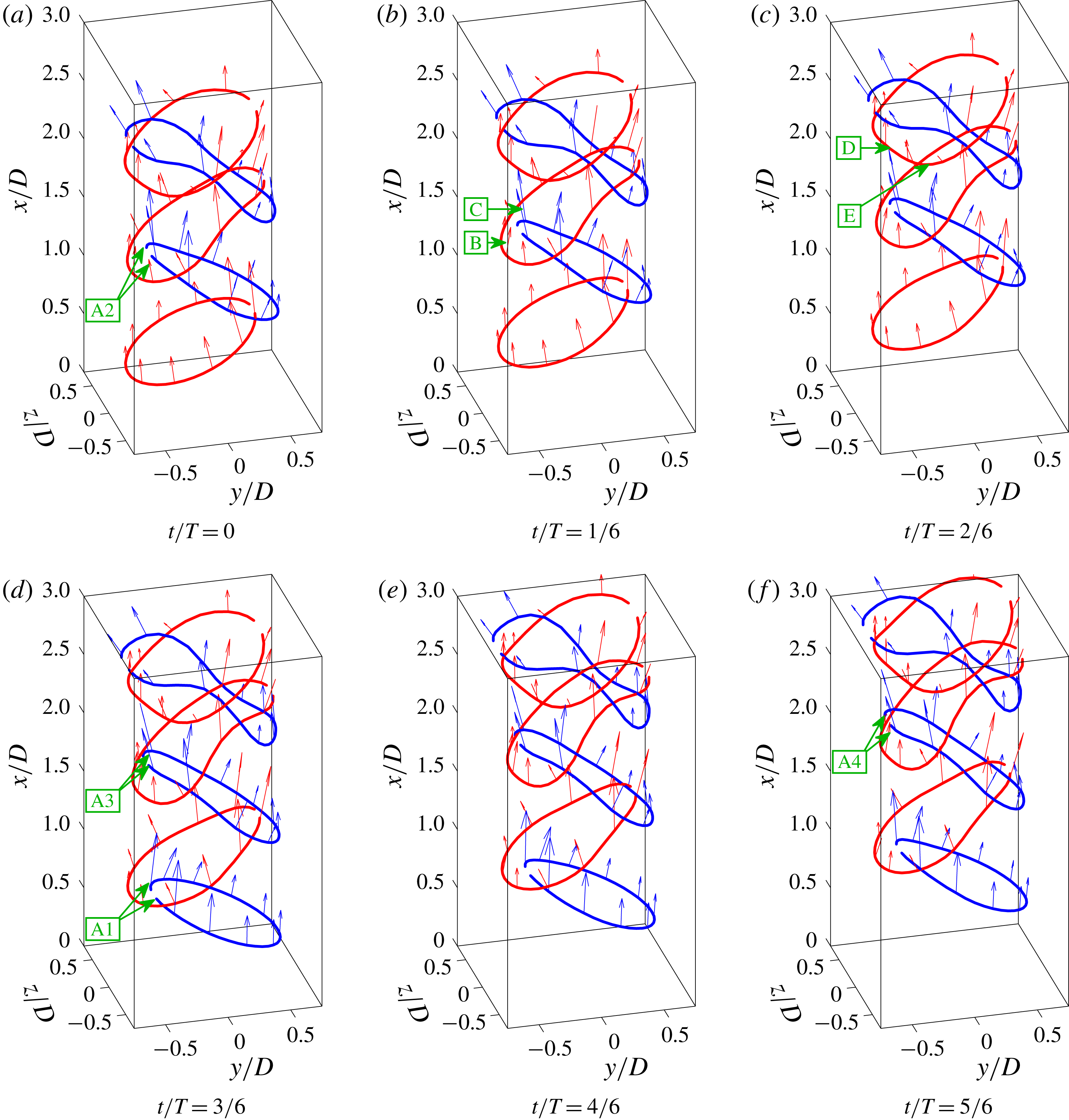
Vortex line locations from the inviscid vortex model, at three points in the forcing cycle. Structures with opposite initial inclination angle and orientation are plotted with different colours to aid identification. Velocity vectors representing only the induced component of velocity, $\boldsymbol{u}_{\boldsymbol{i}}(t)$ , are also plotted at every fourth node location. Annotations identify: A1–A4, the legs of the hairpin are drawn through the arch of the preceding structure; B, the induced component of velocity on the head has a negative radial component and a modest axial component; C, the induced component on the legs has a positive radial component and a large axial component which in combination give rise to the observed dynamics; D, the centre of the hairpin head begins to arch upward under the induced velocity of the legs; E, the shoulders of the hairpin begin to bow outwards in the cross-stream direction resulting in an increasingly square geometry.

3.3 Inviscid vortex line model

Having experimentally characterised the jet in terms of its dominant vortical structures, it is now useful to present results from the inviscid vortex line model introduced in § 2.3 in order to further understand the role of induction in the development of these structures. Figure 11 shows vortex line representations of structures from the inviscid model, at three points in the forcing cycle. Close to the jet exit, the initial inclined ring shape of the structures is clearly shown, with alternating structures plotted with different colours to aid identification. As the model time advances, these structures are advected downstream with a uniform velocity, as well as advecting in the transverse direction due to the applied periodic acoustic advection velocity. The constant downstream advection results in multiple structures distributed in the streamwise direction, separated as in the experiment by a distance of $\unicode[STIX]{x0394}x/D\approx 1$ . While difficult to see in this three-dimensional representation due to the smaller transverse component magnitude, the structures also periodically advect back and forth slightly in the transverse direction. However, except for defining the initial relative locations of the structures, these steady and quasi-steady components of the total advection do nothing to modify the shape or orientation of the structures themselves. It is rather the induced velocity component which results in hairpin deformations as they are advected downstream. In order to understand this contribution, velocity vectors representing only the induced velocity component, $\boldsymbol{u}_{\boldsymbol{i}}(t)$ , are also plotted at every fourth node location.

As the hairpin structures advect downstream they are observed to deform in a number of ways. In particular, however, there is a strong interaction between the open ends of each ring, which represents the lower part of each hairpin’s legs, and the head of the structure immediately downstream. The lower part of each hairpin’s legs begins by trailing the head of the structure immediately downstream (A1 in figure 11). However, these are rapidly pulled upwards (A2 in figure 11) and ultimately through the arch and over the top of the head of the structure immediately downstream (A3 and A4 in figure 11), as a result of the induced velocity from the downstream hairpin head. This effect is made apparent when comparing the size and inclination of the velocity vectors on the legs of one structure and the head of the downstream structure. Higher velocity magnitudes and a positive radial component are observed on the lower part of the legs (C in figure 11), and lower velocity magnitudes and a negative radial component are seen on the heads (B in figure 11).

The lower part of the hairpin legs also induces a reciprocal effect, causing the head of the downstream structure to arch upwards in its centre (D in figure 11), and the shoulders of the structure (the points approximately between the head and legs) to bow downwards in the streamwise and outwards in the cross-stream direction (E in figure 11). The deformation this induces bears strong similarities to the structures observed experimentally in figure 4. Therefore, while this simple model cannot capture the full complexity of the jet dynamics, it does indicate that the increasingly square geometry of the structures as they advect downstream, the increasing hairpin angle and the deformation and eventual break-up of the structure head may all be a result of the interaction between subsequent structures through mutual induction.

The structure dynamics predicted by the vortex model can be further quantified by examining the downstream and radial locations of the filaments and the corresponding evolution of the hairpin inclination angle. The normalised hairpin head and leg locations were defined in a manner similar to those for the experimental results, in this case through the intersection of the closest vortex filament from each structure with the $x$ – $y$ and $x$ – $z$ planes for the head and legs, respectively. The inclination angles were also defined in a similar manner, and calculated from these locations. In order to compare directly with the experimental results, the locations and angles from the vortex model were plotted previously in figures 8 and 9, and are now discussed.

As observed previously in the experimental results, figure 9 shows that the heads are created at a larger radius than the legs due to the transverse flapping of the jet. In the model the radial positioning of the hairpin heads at small downstream distances is correctly replicated primarily through the initialisation of the ring position. The periodic oscillation of head radial position with downstream location is also well captured at moderate downstream distances, through the specified phase relationship of the transverse acoustic advection velocity.

As shown in figure 9, the legs are initially located at smaller radii in comparison with the heads, and as the structures advect downstream they are seen to move further inwards radially. This inward radial movement of the legs is captured correctly by the vortex model which also shows a decrease in radial position with increasing downstream distance. This behaviour in the modelled structures can be attributed to the interaction induced between subsequent structures. As the two legs from a hairpin structure are pulled up and through the head of the downstream structure, they are induced to bunch more closely together. As the hairpin legs bunch together they induce greater velocities on one another and advect more rapidly downstream. Conversely the larger radial location of the hairpin heads means that these experience lower induced velocities, and therefore advect more slowly downstream. In conformity with the experimental results, these differing advection velocities are reflected in both the downstream locations of the head and legs shown in figure 8(a), and also the vortex inclination angles calculated from these in figure 8(b). Therefore, despite its simplistic formulation, the vortex model provides reasonable prediction of the development of the vortex locations in the near field, indicating that the complex dynamics of the hairpin structures is largely driven by induction. The model cannot, however, capture the break-up of the vortices, and therefore the radial locations of the head at large downstream distances are poorly described.

3.4 Root mean square velocity oscillations

Figure 12.

Comparison of normalised components of the RMS velocity between experimental (Exp.) and vortex model (VM) results. Contours are presented in both the $x$ – $y$ plane at $z/D=0$ and the $x$ – $z$ plane at $y/D=0$ .

It is also interesting to examine the velocity field statistics through the root mean square (RMS) velocity oscillations. On an unforced turbulent round jet these would be expected to grow in amplitude with downstream distance as the shear layers develop, reaching modest amplitudes (see for example Pope (Reference Pope2000), § 5.4.1, p. 136). However, the formation of large-scale phase-averaged vortex structures at the jet exit due to acoustic forcing significantly modifies their distribution. To illustrate this, normalised RMS velocity oscillations are plotted in figure 12 on both the $x$ – $y$ and $x$ – $z$ planes from both the experiment (left-hand half of each panel) and the model (right-hand half of each panel). It should be noted that both experimental and model results lack a turbulent fluctuating component, and therefore the RMS components in the present study are representative of the phase-averaged velocity fluctuations, $\sqrt{\overline{\widetilde{\boldsymbol{u}}^{2}}}$ , rather than the more conventional sum of phase-averaged fluctuating and turbulent oscillations, $\sqrt{\overline{(\widetilde{\boldsymbol{u}}+\boldsymbol{ u}^{\prime })^{2}}}$ .

The streamwise component of the RMS velocity, $\sqrt{\overline{\widetilde{u}^{2}}}/u_{e}$ , is presented in figures 12(a) and 12(d) for the $x$ – $y$ and $x$ – $z$ planes, respectively. The $x$ – $y$ plane captures the transverse jet oscillation, and the experimental results show a high-magnitude region close to the jet exit and a lower-magnitude streak which follows the meandering trajectory of the vortex structures as these advect downstream. In the $x$ – $z$ plane there are no large oscillations at the base of the jet in the experimental results, but a similar lower-magnitude streak appears along the shear layer, with the shape of this streak again closely following the vortex trajectories observed previously. It is also worth commenting on the magnitude of oscillations. Experimentally RMS velocities are observed up to approximately 30 % of the bulk flow velocity, which is significantly larger than the magnitude of turbulent fluctuations in the near field of an unforced jet.

The model results in the right-hand half of the panels of figure 12(a,d) show artificially high regions of oscillating velocity in the near field close to the jet axis in both planes of interest. These regions result from the artificial method of structure formation used in the current model. The sudden placement of structures, rather than directly modelling the roll-up process, gives rise to large oscillations over the forcing cycle close to the jet exit. However, as our current interest is in understanding structure development, accepting this deficiency the model does appear to capture some important features of the downstream RMS distribution, replicating to a certain degree the high-magnitude streaks associated with the meandering path of the vortex cores, and the approximate magnitude of the RMS velocity.

The transverse component of oscillating velocity, $\sqrt{\overline{\widetilde{v}^{2}}}/u_{e}$ , is shown in figures 12(b) and 12(e) for the $x$ – $y$ and $x$ – $z$ planes, respectively. From the experimental results, the fields are dominated by a series of high-magnitude regions, which again follow the trajectory of the vortex cores. The pinching and expanding of these high-magnitude regions in the $x$ – $y$ plane with increasing downstream distance result from the combination of the induced velocity from the vortex cores either combining with or cancelling out the transverse acoustic velocity oscillations. This results in a distinctive patternation of the field, the essential features of which are replicated relatively well by the vortex model. However, the vortex model is not capable of accurately capturing the vortex breakdown, and therefore larger discrepancies are seen with increasing downstream distance ( $x/D>2$ ). Similarly, important features of the transverse component in the $x$ – $z$ plane, such as the inwardly inclined high-magnitude streaked regions close to the jet shear layers and the low-magnitude elliptical regions along the jet centreline, are also represented relatively well by the vortex model in the near field.

Finally, reasonable agreement in the distribution and amplitude of RMS velocity is also observed for the cross-stream component, $\sqrt{\overline{\widetilde{w}^{2}}}/u_{e}$ , as shown in figure 12(c,f).

The reasonably good agreement between experimental and numerical results in terms of both distribution and amplitude of velocity oscillations demonstrates that the velocity field statistics are dominated by the large-scale hairpin structures, with the pronounced departures from the behaviour of an unforced jet driven by velocity induced by the coherent hairpin structures in addition to the contribution from the acoustic field, rather than by jet instabilities or other viscous effects.

3.5 Spectral analysis

Figure 13.

Weighted phase of vorticity fluctuations in the $y$ – $z$ plane at different downstream locations, showing the response at the forcing frequency and second and third harmonics. The colour in each panel represents the phase angle of the fluctuation at the measurement location, and the brightness represents the oscillation magnitude.

In order to further analyse the spectral content of the velocity gradient field, the weighted phase of vorticity fluctuations was calculated in $y$ – $z$ planes at different downstream locations, shown in figure 13. The weighted phase calculation used an approach similar to that of Hauser et al. (Reference Hauser, Lorenz and Sattelmayer2011), in which the fast Fourier transform of the vorticity magnitude fluctuation at each measurement point within each plane of interest was taken, before using these complex values to calculate the magnitude, $|\unicode[STIX]{x1D74E}(f)|$ , and phase, $\unicode[STIX]{x1D6F9}_{\unicode[STIX]{x1D714}}(f)$ , of vorticity oscillations for different harmonic components ( $f=mf_{f}$ , where $m$ is an integer). Weighted phase images were created at integer values of the forcing frequency by using colour to denote the phase angle of the oscillations at each measurement location, and brightness to denote amplitude. Through this weighting the phase variation is only discernible in regions with a significant fluctuation amplitude, providing a useful way of understanding the most significant vorticity oscillations. Zero padding was used in order to ensure frequency bins were located at integer multiples of the forcing frequency, and Hann windowing was employed in order to reduce dependence on the limited sample size. Finally, it is also important to note that the cyclic colour map was selected to be perceptibly uniform prior to the brightness weighting process (Thyng et al. Reference Thyng, Greene, Hetland, Zimmerle and DiMarco2016).

The development of the vortex structures as they advect downstream can be understood by looking from left to right on the figure. Images in the top row are brightest, indicating that the vorticity field is dominated by oscillations at the first harmonic. Crescent-shaped regions in this row correspond to the head and legs of the vortex structures, which are clearly visible on each side of the $y$ axis. The phase colouring shows these structures are in anti-phase with each other at each downstream location, corresponding to the previously observed staggered downstream locations of the vortex core heads. As the hairpin structures are advected downstream they can be seen to deform, from initially round close to the jet exit to increasingly square. It is also interesting to note that immediately downstream of the jet exit, vorticity fluctuations along structures either side of the $y$ axis are in phase, but as these structures are advected downstream, they exhibit phase variations along each structure. These waves are likely to arise as a result of the observed mutual interaction of the structures with vortices downstream.

While vorticity fluctuations at the second harmonic are in general significantly lower in amplitude in comparison with the fundamental frequency, the middle row of weighted phase images is marked by two bright points between $1<x/D<2$ , which lie on the $y$ axis at $x/D=\pm 0.5$ . These two points represent the passage of the hairpin leg structures, but these peaks are now centred at $f/f_{f}=2$ , due to the formation of two structures every forcing cycle. The way that these hairpin structures are interwoven means that only a relatively small region of the flow experiences a strong frequency doubling due to the leg vortices advecting past the same volumetric location. The figure also demonstrates how short-lived these structures are, with the magnitude of the other harmonic components becoming similar to that of the principal components further downstream, $x/D\geqslant 2.5$ , which is indicative of their rapid subsequent breakdown.