1 Introduction
Processes of contact between deformable bodies abound in industry and everyday life. A few simple examples are brake pads in contact with wheels, tyres on roads, and pistons with skirts. Because of the importance of contact processes in structural and mechanical systems, considerable effort has been put into their modelling, analysis and numerical simulations. The literature on this field is extensive. The publications in the engineering literature are often concerned with specific settings, geometries or materials. Their aim is usually related to particular applied aspects of the problems. The publications on mathematical literature are concerned with the mathematical structures which underlie general contact problems with different constitutive laws, varied geometries and different contact conditions. They deal with the variational analysis of the corresponding models of contact. Once existence, uniqueness or non-uniqueness, and stability of solutions have been established, related important questions arise, such as numerical analysis of the solutions and how to construct reliable and efficient algorithms for their numerical approximations with guaranteed accuracy.
The first recognized publication on contact between deformable bodies was that of Hertz (Reference Hertz1882). This was followed by Signorini (Reference Signorini1933), who posed the problem in what is now termed a variational form. The Signorini problem was theoretically investigated by Fichera (Reference Fichera1964, Reference Fichera and Truesdell1972). However, the general mathematical development for problems arising in contact mechanics began with the monograph by Duvaut and Lions (Reference Duvaut and Lions1976), who presented variational formulations of several contact problems and proved some basic existence and uniqueness results. A comprehensive treatment of unilateral contact problems, for linear and nonlinear elastic materials, and for both frictionless and frictional contact, was provided by Kikuchi and Oden (Reference Kikuchi and Oden1988), who covered mathematical modelling of the contact phenomena, numerical analysis and implementation of numerical algorithms. A systematic coverage of numerical methods for solving unilateral contact problems, for both frictionless and frictional contact of linearly elastic materials, can be found in Hlaváček, Haslinger, Nečas and Lovíšek (Reference Hlaváček, Haslinger, Nečas and Lovíšek1988), and an updated account of numerical methods for unilateral contact problems is given in Haslinger, Hlaváček and Nečas (Reference Haslinger, Hlaváček, Nečas, Ciarlet and Lions1996).
For frictionless Signorini contact between two elastic bodies we refer to Haslinger and Hlaváček (Reference Haslinger and Hlaváček1980, Reference Haslinger and Hlaváček1981a , Reference Haslinger and Hlaváček1981b ), who proved the existence and uniqueness of a weak solution and provided numerical algorithms to solve the corresponding nonlinear boundary value problems. By introducing dual Lagrange multipliers for contact forces, a variational inequality in displacement can be reformulated as a saddle-point problem, which can be solved by semi-smooth Newton methods with a primal–dual active set strategy; see Wohlmuth and Krause (Reference Wohlmuth and Krause2003), Hüeber and Wohlmuth (Reference Hüeber and Wohlmuth2005a , Reference Hüeber and Wohlmuth2005b ), Wriggers and Fischer (Reference Wriggers and Fischer2005) and the survey article by Wohlmuth (Reference Wohlmuth2011) for a summary account. Multigrid methods can be used to efficiently solve contact problems; e.g. Kornhuber and Krause (Reference Kornhuber and Krause2001). For an optimal a priori error estimate for numerical solutions of the Signorini contact problem, we refer to the recent paper by Drouet and Hild (Reference Drouet and Hild2015). A few steps in the mathematical analysis for models involving time-dependent unilateral contact between a deformable body and a rigid obstacle were made by Sofonea, Renon and Shillor (Reference Sofonea, Renon and Shillor2004) and Renon, Montmitonnet and Laborde (Reference Renon, Montmitonnet and Laborde2005). The quasistatic process of frictionless unilateral contact between a moving rigid obstacle and a viscoelastic body has been considered by Matei, Sitzmann, Willner and Wohlmuth (Reference Matei, Sitzmann, Willner and Wohlmuth2017). Their model leads to a variational formulation with dual Lagrange multipliers. They obtained the existence of a solution by using a time discretization method combined with a saddle-point argument. Moreover, they used an efficient algorithm based on a primal–dual active set strategy, and presented three-dimensional numerical examples using the mortar method to discretize the contact constraints, without increasing the algebraic system size.
Monographs and books on mathematical problems in contact mechanics also include those by Panagiotopoulos (Reference Panagiotopoulos1985) for mechanical background, mathematical modelling and analysis, and engineering application, Han and Sofonea (Reference Han and Sofonea2002) for mathematical modelling and analysis, as well as convergence analysis and optimal order error estimates of numerical methods for quasistatic contact problems of elastic, viscoelastic and viscoplastic materials, Shillor, Sofonea and Telega (Reference Shillor, Sofonea and Telega2004) for mathematical modelling and analysis of contact problems, Eck, Jarušek and Krbec (Reference Eck, Jarušek and Krbec2005) for variational analysis of unilateral contact problems in elasticity and viscoelasticity, and Capatina (Reference Capatina2014) for a mathematical study of certain frictional contact problems. The books by Laursen (Reference Laursen2002), Wriggers (Reference Wriggers2006) and Wriggers and Laursen (Reference Wriggers and Laursen2007) focus on numerical algorithms for solving contact problems and on engineering applications. The above references deal with variational inequality formulations of the problems in contact mechanics. In comparison, hemivariational inequality formulations are used in the study of contact problems with non-monotone mechanical relations in some more recent monographs, and we mention Panagiotopoulos (Reference Panagiotopoulos1993) for mathematical modelling, analysis and numerical simulation of contact problems, Migórski, Ochal and Sofonea (Reference Migórski, Ochal and Sofonea2013) for mathematical modelling and analysis of various contact problems, and Sofonea and Migórski (Reference Sofonea and Migórski2018) for the modelling and analysis of static, history-dependent and evolutionary contact problems in the form of a special class of hemivariational inequalities called variational–hemivariational inequalities, in which both convex and non-convex functions are present.
Inequality problems in contact mechanics can be loosely classified into two main families: the family of variational inequalities, which is concerned with convex functionals (potentials), and the family of hemivariational inequalities, which is concerned with non-convex functionals (superpotentials). Some of the model problems considered in this paper are special kinds of inequalities, known as variational–hemivariational inequalities. In a variational–hemivariational inequality, we have the presence of both non-convex functionals and convex functionals. When the convex functionals are dropped from a general variational–hemivariational inequality, we have a ‘pure’ hemivariational inequality. Alternatively, when the non-convex functionals are dropped, we have a ‘pure’ variational inequality. Nevertheless, for simplicity, sometimes in this paper we use the term hemivariational inequality for both ‘pure’ hemivariational and variational–hemivariational inequalities. The theoretical results on the variational–hemivariational inequalities naturally lead to those for the corresponding variational and hemivariational inequalities.
Variational and hemivariational inequalities represent a powerful tool in the study of a large number of nonlinear boundary value problems. The theory of variational inequalities was first developed in the early 1960s, based on arguments of monotonicity and convexity, and properties of the subdifferential of a convex function. Representative references on mathematical studies of variational inequalities include Lions and Stampacchia (Reference Lions and Stampacchia1967), Brézis (Reference Brézis1972), Baiocchi and Capelo (Reference Baiocchi and Capelo1984) and Kinderlehrer and Stampacchia (Reference Kinderlehrer and Stampacchia2000), to name a few. Hemivariational inequalities were first introduced in the early 1980s by Panagiotopoulos in the context of applications in engineering problems. Studies of hemivariational inequalities can be found in several comprehensive references, for example Panagiotopoulos (Reference Panagiotopoulos1993), Naniewicz and Panagiotopoulos (Reference Naniewicz and Panagiotopoulos1995) and Migórski, Ochal and Sofonea (Reference Migórski, Ochal and Sofonea2013), as well as in the volume edited by Han, Migórski and Sofonea (Reference Han, Migórski and Sofonea2015).
Since a closed-form solution formula can rarely be obtained for a general variational inequality or hemivariational inequality, numerical methods are essentially the only way to solve the inequality problems in practice. References on numerical analysis of general variational inequalities include the books by Glowinski, Lions and Trémolières (Reference Glowinski, Lions and Trémolières1981) and Glowinski (Reference Glowinski1984), and references on variational inequalities for contact problems include those of Kikuchi and Oden (Reference Kikuchi and Oden1988), Hlaváček, Haslinger, Nečas and Lovíšek (Reference Hlaváček, Haslinger, Nečas and Lovíšek1988), Haslinger, Hlaváček and Nečas (Reference Haslinger, Hlaváček, Nečas, Ciarlet and Lions1996) and Han and Sofonea (Reference Han and Sofonea2002). In comparison, the size of the literature on the numerical analysis of hemivariational inequalities is much smaller. The book by Haslinger, Miettinen and Panagiotopoulos (Reference Haslinger, Miettinen and Panagiotopoulos1999) is devoted to the finite element approximations of hemivariational inequalities, where convergence of numerical methods is discussed; however, no error estimates of the numerical solutions are derived. In recent years there have been efforts by various researchers to derive error estimates for numerical solutions of hemivariaional inequalities, and initially, only sub-optimal error estimates were reported. Han, Migórski and Sofonea (Reference Han, Migórski and Sofonea2014) were the first to give an optimal order error estimate for linear finite element solutions in solving hemivariational or variational–hemivariational inequalities. Then Barboteu, Bartosz, Han and Janiczko (Reference Barboteu, Bartosz, Han and Janiczko2015) derived an optimal order error estimate for the numerical solution of a hyperbolic hemivariational inequality arising in dynamic contact when the linear finite element method is used for the spatial discretization and the backward Euler finite difference is used for the time derivative. With similar derivation techniques, various authors derived optimal order error estimates for the linear finite element method of a few individual hemivariational or variational–hemivariational inequalities, in several papers. More recently, general frameworks of convergence theory and error estimation for hemivariational or variational–hemivariational inequalities have been developed; see Han, Sofonea and Barboteu (Reference Han, Sofonea and Barboteu2017) and Han, Sofonea and Danan (Reference Han, Sofonea and Danan2018) for internal numerical approximations of general hemivariational and variational–hemivariational inequalities, and Han (Reference Han2018) for both internal and external numerical approximations of general hemivariational and variational–hemivariational inequalities. In these recent papers, convergence is shown for numerical solutions by internal or external approximation schemes under minimal solution regularity condition, Céa-type inequalities are derived that serve as the starting point for error estimation for hemivariational and variational–hemivariational inequalities arising in contact mechanics, and optimal order error estimates for the linear finite element solutions are obtained.
The aim of this survey paper is to provide the state of the art on numerical analysis of some representative mathematical models which describe the contact of a deformable body with an obstacle, the so-called foundation, in the framework of the linearized strain theory. We present models for the processes, list the assumptions on the data and derive their weak formulation, which is in the form of a hemivariational inequality. We have tried to make this paper self-contained. Therefore, in addition to the numerical analysis of the contact models, we review the necessary background on the analysis of the related hemivariational inequalities, including existence and uniqueness results.
The paper is organized as follows. In Section 2 we introduce three representative models of contact and describe them in full detail. Then we list the assumptions on the data and state the weak formulations of the models, which are in the form of an elliptic, a history-dependent and an evolutionary hemivariational inequality, respectively. In Section 3 we present preliminary material on basic notions and results from non-smooth analysis that will be needed later in the well-posedness study and numerical analysis of the hemivariational inequalities. In addition, we also recall Banach’s fixed-point theorem as well as Gronwall’s inequalities in both the continuous version and discrete version. In Sections 4–6 we present well-posedness results and consider numerical approximations of three abstract hemivariational inequalities of the elliptic, history-dependent and evolutionary types. The results on the abstract hemivariational inequalities are applied in Sections 7–9 on the contact models, leading to statements of well-posedness of the contact problems, of convergence and optimal order error estimates of numerical methods. Numerical simulation results are shown to provide numerical evidence of the theoretically predicted first-order error estimate in the energy norm for linear finite element solutions. In Section 10, we comment on future research topics on the numerical solution of hemivariational inequalities, especially those arising in contact mechanics.
2 Three representative contact problems
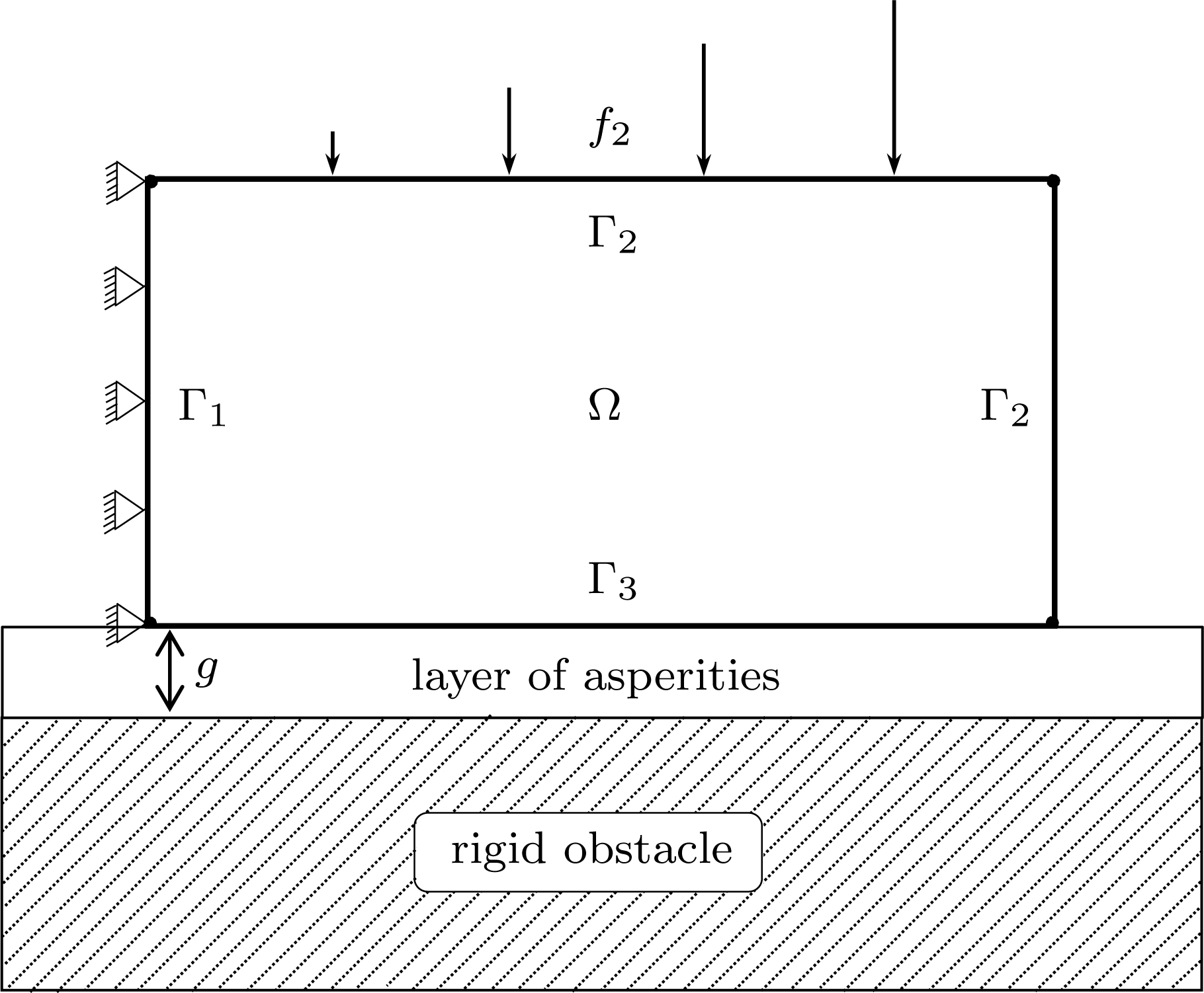
Physical setting and mathematical models.
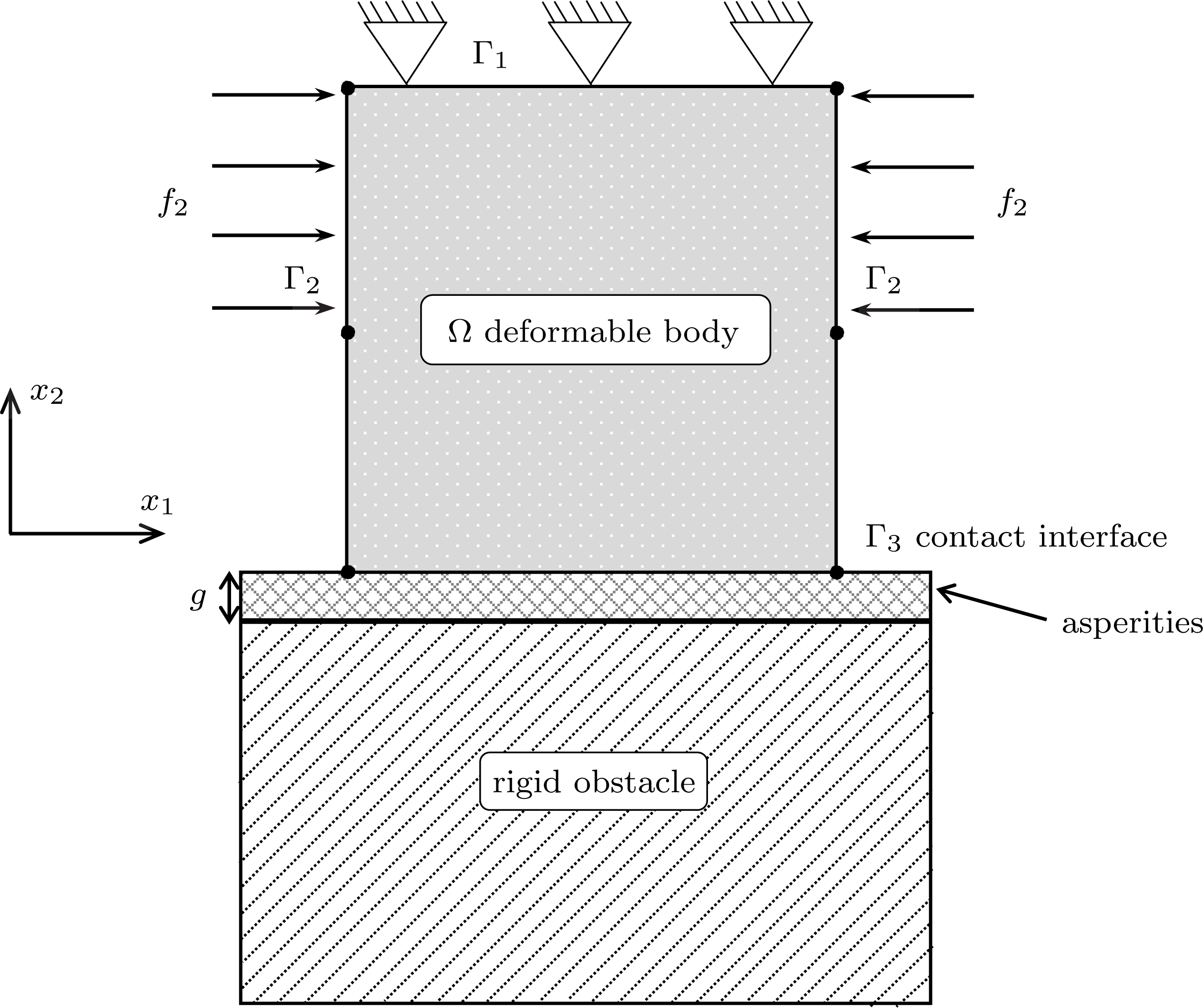
A large number of processes of contact arising in various engineering applications can be cast in the following general physical setting: a deformable body is subjected to the action of body forces and surface tractions, is clamped on part of its surface and is in contact with a foundation on another part of its surface. We are interested in describing the evolution of the mechanical state of the body and, to this end, the first step is to construct a mathematical model which describes the physical setting above. Here and everywhere in this work, by a mathematical model we understand a system of partial differential equations with associated boundary conditions and with possibly initial conditions, for a specific contact process. Such models are constructed based on the general principles of solid mechanics, which can be found in Ciarlet (Reference Ciarlet1988), Khludnev and Sokolowski (Reference Khludnev and Sokolowski1997) and Temam and Miranville (Reference Temam and Miranville2001), for instance.
To present a mathematical model in contact mechanics we need to combine several relations: the constitutive law, the balance equation, the boundary conditions, the interface laws, and for evolutionary problems, the initial conditions. Recall that a constitutive law represents a relation between the stress
 $\unicode[STIX]{x1D748}$
and the strain
 $\unicode[STIX]{x1D73A}$
, and the relation may involve derivatives and/or integrals of the the stress and/or strain. The constitutive law describes the mechanical reaction of the material with respect to the action of body forces and boundary tractions. Although the constitutive laws must satisfy some basic axioms and invariance principles, they originate mostly from experiments. We refer the reader to Han and Sofonea (Reference Han and Sofonea2002) for a general description of several diagnostic experiments which provide information needed in constructing constitutive laws for specific materials. The balance equation for the stress field leads either to the equation of motion (used in the modelling of dynamic processes, i.e. processes in which the inertial terms are not neglected) or to the equation of equilibrium (used in the modelling of static and quasistatic processes, i.e. processes in which the inertial terms are neglected). The boundary conditions usually involve the displacement and the surface tractions. They express the fact that the body is held fixed on a part of the boundary and is acted upon by external forces on the other part. The interface laws are to be prescribed on the potential contact surface. These are divided naturally into conditions in the normal direction (called contact conditions) and those in the tangential directions (called friction laws). A comprehensive description of the interface laws used in the mathematical literature dedicated to modelling of contact problems can be found in Sofonea and Matei (Reference Sofonea and Matei2012) and Migórski, Ochal and Sofonea (Reference Migórski, Ochal and Sofonea2013).
Basic notation.
In order to introduce the contact models, we let
 $\unicode[STIX]{x1D6FA}$
be the reference configuration of the body, assumed to be an open, bounded, connected set in
 $\mathbb{R}^{d}$
with a Lipschitz boundary
 $\unicode[STIX]{x1D6E4}=\unicode[STIX]{x2202}\unicode[STIX]{x1D6FA}$
. The dimension
 $d=2$
or
 $3$
for applications. The closure of
 $\unicode[STIX]{x1D6FA}$
in
 $\mathbb{R}^{d}$
is denoted by
 $\overline{\unicode[STIX]{x1D6FA}}$
. To describe the boundary conditions, we split the boundary
 $\unicode[STIX]{x1D6E4}$
into three disjoint, measurable parts
 $\unicode[STIX]{x1D6E4}_{1}$
,
 $\unicode[STIX]{x1D6E4}_{2}$
and
 $\unicode[STIX]{x1D6E4}_{3}$
. Here,
 $\operatorname{meas}\,(\unicode[STIX]{x1D6E4}_{1})>0$
and
 $\operatorname{meas}\,(\unicode[STIX]{x1D6E4}_{3})>0$
, whereas
 $\unicode[STIX]{x1D6E4}_{2}$
is allowed to be empty. We use boldface letters for vectors and tensors, such as the outward unit normal
 $\unicode[STIX]{x1D742}$
on
 $\unicode[STIX]{x1D6E4}$
. A typical point in
 $\mathbb{R}^{d}$
is denoted by
 $\boldsymbol{x}=(x_{i})$
. The indices
 $i$
,
 $j$
,
 $k$
,
 $l$
run between
 $1$
and
 $d$
, and, unless stated otherwise, the summation convention over repeated indices is implied. An index that follows a comma indicates a partial derivative with respect to the corresponding component of the spatial variable
 $\boldsymbol{x}$
. For integrals, we use
 $\text{d}x$
for the infinitesimal volume element in
 $\unicode[STIX]{x1D6FA}$
and
 $\text{d}a$
for the infinitesimal surface element on
 $\unicode[STIX]{x1D6E4}$
. For a time-dependent contact problem, the time interval of interest will be denoted by
 $I$
, which can be bounded or unbounded. A dot above a variable will represent the time derivative of the variable.
We are interested in mathematical models which describe the evolution or the equilibrium of the mechanical state of the body within the framework of the linearized strain theory. We use the symbols
 $\boldsymbol{u}$
,
 $\unicode[STIX]{x1D748}$
and
 $\unicode[STIX]{x1D73A}=\unicode[STIX]{x1D73A}(\boldsymbol{u})$
for the displacement vector, the stress tensor and the linearized strain tensor, respectively. The components of the linearized strain tensor
 $\unicode[STIX]{x1D73A}(\boldsymbol{u})$
are given by
 $$\begin{eqnarray}\unicode[STIX]{x1D700}_{ij}(\boldsymbol{u})=(\unicode[STIX]{x1D73A}(\boldsymbol{u}))_{ij}=\displaystyle \frac{1}{2}\,(u_{i,j}+u_{j,i}),\end{eqnarray}$$
where
 $u_{i,j}=\unicode[STIX]{x2202}u_{i}/\unicode[STIX]{x2202}x_{j}$
. These are functions of the spatial variable
 $\boldsymbol{x}$
, and of the time variable
 $t$
as well for time-dependent problems. Nevertheless, in what follows we do not indicate explicitly the dependence of these quantities on
 $\boldsymbol{x}$
and
 $t$
: for example, we write
 $\unicode[STIX]{x1D748}$
instead of
 $\unicode[STIX]{x1D748}(\boldsymbol{x})$
or
 $\unicode[STIX]{x1D748}(\boldsymbol{x},t)$
. The displacement
 $\boldsymbol{u}$
and the stress
 $\unicode[STIX]{x1D748}$
play the roles of unknowns in the contact problems.
We let
 $\mathbb{S}^{d}$
denote the space of second-order symmetric tensors on
 $\mathbb{R}^{d}$
. Equivalently,
 $\mathbb{S}^{d}$
can be viewed as the space of symmetric matrices of order
 $d$
. The canonical inner products and the corresponding norms on
 $\mathbb{R}^{d}$
and
 $\mathbb{S}^{d}$
are given by
 $$\begin{eqnarray}\displaystyle \boldsymbol{u}\cdot \boldsymbol{v} & = & \displaystyle u_{i}v_{i},\quad \Vert \boldsymbol{v}\Vert =(\boldsymbol{v}\cdot \boldsymbol{v})^{1/2}\quad \text{for all}~\boldsymbol{u}=(u_{i}),\boldsymbol{v}=(v_{i})\in \mathbb{R}^{d},\end{eqnarray}$$
 $$\begin{eqnarray}\displaystyle \unicode[STIX]{x1D748}\cdot \unicode[STIX]{x1D749} & = & \displaystyle \unicode[STIX]{x1D70E}_{ij}\unicode[STIX]{x1D70F}_{ij},\quad \Vert \unicode[STIX]{x1D749}\Vert =(\unicode[STIX]{x1D749}\cdot \unicode[STIX]{x1D749})^{1/2}\quad \text{for all}~\unicode[STIX]{x1D748}=(\unicode[STIX]{x1D70E}_{ij}),\unicode[STIX]{x1D749}=(\unicode[STIX]{x1D70F}_{ij})\in \mathbb{S}^{d},\end{eqnarray}$$
respectively. We use
 $\mathbf{0}$
for the zero element of the spaces
 $\mathbb{R}^{d}$
and
 $\mathbb{S}^{d}$
.
Function spaces.
We will use the standard notation for Sobolev and Lebesgue spaces over
 $\unicode[STIX]{x1D6FA}$
or on
 $\unicode[STIX]{x1D6E4}$
. In particular, we will use the spaces
 $L^{2}(\unicode[STIX]{x1D6FA};\mathbb{R}^{d})$
,
 $L^{2}(\unicode[STIX]{x1D6E4}_{2};\mathbb{R}^{d})$
,
 $L^{2}(\unicode[STIX]{x1D6E4}_{3};\mathbb{R}^{d})$
and
 $H^{1}(\unicode[STIX]{x1D6FA};\mathbb{R}^{d})$
, endowed with their canonical inner products and associated norms. For an element
 $\boldsymbol{v}\in H^{1}(\unicode[STIX]{x1D6FA};\mathbb{R}^{d})$
we write
 $\boldsymbol{v}$
for its trace
 $\unicode[STIX]{x1D6FE}\boldsymbol{v}\in L^{2}(\unicode[STIX]{x1D6FA};\mathbb{R}^{d})$
on
 $\unicode[STIX]{x1D6E4}$
. Define the function spaces
 $$\begin{eqnarray}\displaystyle V & = & \displaystyle \{\boldsymbol{v}\in H^{1}(\unicode[STIX]{x1D6FA};\mathbb{R}^{d})\mid \boldsymbol{v}=\mathbf{0}~\text{on }\unicode[STIX]{x1D6E4}_{1}\},\end{eqnarray}$$
 $$\begin{eqnarray}\displaystyle Q & = & \displaystyle \{\unicode[STIX]{x1D748}=(\unicode[STIX]{x1D70E}_{ij})\mid \unicode[STIX]{x1D70E}_{ij}=\unicode[STIX]{x1D70E}_{ji}\in L^{2}(\unicode[STIX]{x1D6FA})\},\end{eqnarray}$$
for the displacement and the stress field, respectively. These are real Hilbert spaces endowed with the inner products
 $$\begin{eqnarray}(\boldsymbol{u},\boldsymbol{v})_{V}=\int _{\unicode[STIX]{x1D6FA}}\unicode[STIX]{x1D73A}(\boldsymbol{u})\cdot \unicode[STIX]{x1D73A}(\boldsymbol{v})\,\text{d}x,\quad (\unicode[STIX]{x1D748},\unicode[STIX]{x1D749})_{Q}=\int _{\unicode[STIX]{x1D6FA}}\unicode[STIX]{x1D748}\cdot \unicode[STIX]{x1D749}\,\text{d}x.\end{eqnarray}$$
The corresponding norms on the spaces are denoted by
 $\Vert \cdot \Vert _{V}$
and
 $\Vert \cdot \Vert _{Q}$
, respectively. Since
 $\operatorname{meas}\,(\unicode[STIX]{x1D6E4}_{1})>0$
, Korn’s inequality holds (see Nečas and Hlaváček Reference Nečas and Hlaváček1981, p. 79):
 $$\begin{eqnarray}\Vert \boldsymbol{v}\Vert _{H^{1}(\unicode[STIX]{x1D6FA};\mathbb{R}^{d})}\leq c\,\Vert \unicode[STIX]{x1D73A}(\boldsymbol{v})\Vert _{Q}\quad \text{for all}~\boldsymbol{v}\in V,\end{eqnarray}$$
for some constant
 $c>0$
. Thus,
 $\Vert \cdot \Vert _{V}$
defines a norm on
 $V$
that is equivalent to the standard
 $H^{1}(\unicode[STIX]{x1D6FA};\mathbb{R}^{d})$
-norm. We will also use the function space
 $$\begin{eqnarray}H=L^{2}(\unicode[STIX]{x1D6FA};\mathbb{R}^{d})\end{eqnarray}$$
with the canonical inner product and norm.
We let
 $V^{\ast }$
denote the dual of the space
 $V$
and
 $\langle \cdot ,\cdot \rangle$
the corresponding duality pairing. For any element
 $\boldsymbol{v}\in V$
, we let
 $v_{\unicode[STIX]{x1D708}}$
and
 $\boldsymbol{v}_{\unicode[STIX]{x1D70F}}$
denote its normal and tangential components on
 $\unicode[STIX]{x1D6E4}$
given by
 $v_{\unicode[STIX]{x1D708}}=\boldsymbol{v}\cdot \unicode[STIX]{x1D742}$
and
 $\boldsymbol{v}_{\unicode[STIX]{x1D70F}}=\boldsymbol{v}-v_{\unicode[STIX]{x1D708}}\unicode[STIX]{x1D742}$
, respectively. For a regular function
 $\unicode[STIX]{x1D748}:\overline{\unicode[STIX]{x1D6FA}}\rightarrow \mathbb{S}^{d}$
, we let
 $\unicode[STIX]{x1D70E}_{\unicode[STIX]{x1D708}}$
and
 $\unicode[STIX]{x1D748}_{\unicode[STIX]{x1D70F}}$
denote its normal and tangential components on
 $\unicode[STIX]{x1D6E4}$
, i.e.
 $\unicode[STIX]{x1D70E}_{\unicode[STIX]{x1D708}}=(\unicode[STIX]{x1D748}\unicode[STIX]{x1D742})\cdot \unicode[STIX]{x1D742}$
and
 $\unicode[STIX]{x1D748}_{\unicode[STIX]{x1D70F}}=\unicode[STIX]{x1D748}\unicode[STIX]{x1D742}-\unicode[STIX]{x1D70E}_{\unicode[STIX]{x1D708}}\unicode[STIX]{x1D742}$
, and we recall that the following Green’s formula holds:
 $$\begin{eqnarray}\int _{\unicode[STIX]{x1D6FA}}\,\unicode[STIX]{x1D748}\cdot \unicode[STIX]{x1D73A}(\boldsymbol{v})\,\text{d}x+\int _{\unicode[STIX]{x1D6FA}}\,\text{Div}\,\unicode[STIX]{x1D748}\cdot \boldsymbol{v}\,\text{d}x=\int _{\unicode[STIX]{x1D6E4}}\unicode[STIX]{x1D748}\unicode[STIX]{x1D742}\cdot \boldsymbol{v}\,\text{d}a\quad \text{for all}~\boldsymbol{v}\in H^{1}(\unicode[STIX]{x1D6FA},\mathbb{R}^{d}).\end{eqnarray}$$
We also recall that
 $$\begin{eqnarray}\Vert \boldsymbol{v}\Vert _{L^{2}(\unicode[STIX]{x1D6E4};\mathbb{R}^{d})}\leq \Vert \unicode[STIX]{x1D6FE}\Vert \Vert \boldsymbol{v}\Vert _{V}\quad \text{for all}~\boldsymbol{v}\in V,\end{eqnarray}$$
where
 $\Vert \unicode[STIX]{x1D6FE}\Vert$
represents the norm of the trace operator
 $\unicode[STIX]{x1D6FE}:V\rightarrow L^{2}(\unicode[STIX]{x1D6E4};\mathbb{R}^{d})$
. Inequality (2.7) represents a consequence of the Sobolev trace theorem.
We introduce a space of fourth-order tensors:
 $$\begin{eqnarray}\mathbf{Q_{∞}}=\{{\mathcal{E}}=(e_{ijkl})\mid e_{ijkl}=e_{jikl}=e_{klij}\in L^{\infty }(\unicode[STIX]{x1D6FA}),~1\leq i,j,k,l\leq d\}.\end{eqnarray}$$
It is a Banach space endowed with the norm
 $$\begin{eqnarray}\Vert {\mathcal{E}}\Vert _{\mathbf{Q_{∞}}}=\max _{1\leq i,j,k,l\leq d}\Vert e_{ijkl}\Vert _{L^{\infty }(\unicode[STIX]{x1D6FA})}.\end{eqnarray}$$
It is easy to see that
 $$\begin{eqnarray}\Vert {\mathcal{E}}\unicode[STIX]{x1D749}\Vert _{Q}\leq d\,\Vert {\mathcal{E}}\Vert _{\mathbf{Q_{∞}}}\Vert \unicode[STIX]{x1D749}\Vert _{Q}\quad \text{for all}~{\mathcal{E}}\in \mathbf{Q_{∞}},\,\unicode[STIX]{x1D749}\in Q.\end{eqnarray}$$
Below,
 $\mathbb{N}$
represents the set of positive integers,
 $I$
denotes either a bounded interval of the form
 $[0,T]$
with
 $T>0$
, or the unbounded interval
 $\mathbb{R}_{+}=[0,+\infty )$
and
 $X$
will be a Banach space. We let
 $C(I;X)$
denote the space of continuous functions on
 $I$
with values in
 $X$
. In addition, we let
 $C^{1}(I;X)$
denote the space of continuously differentiable functions on
 $I$
with values in
 $X$
. Therefore,
 $v\in C^{1}(I;X)$
if and only if
 $v\in C(I;X)$
and
 $\dot{v}\in C(I;X)$
where
 $\dot{v}$
represents the time derivative of the function
 $v$
. In addition, for a subset
 $K\subset X$
, we use the notation
 $C(I;K)$
for the set of functions defined on
 $I$
with values in
 $K$
.
In the case
 $I=[0,T]$
the space
 $C(I;X)$
is equipped with the norm
 $$\begin{eqnarray}\Vert v\Vert _{C([0,T];X)}=\max _{t\in [0,T]}\,\Vert v(t)\Vert _{X}.\end{eqnarray}$$
It is well known that
 $C(I;X)$
is a Banach space. In the case
 $I=\mathbb{R}_{+}$
,
 $C(I;X)$
can be organized in a canonical way as a Fréchet space, i.e., it is a complete metric space in which the corresponding topology is induced by a countable family of seminorms. The convergence of a sequence
 $\{{v_{k}\}}_{k}$
to an element
 $v$
, in the space
 $C(\mathbb{R}_{+};X)$
, can be described as follows:
 $$\begin{eqnarray}\displaystyle & & \displaystyle v_{k}\rightarrow v\text{ in }C(\mathbb{R}_{+};X)\text{ as }k\rightarrow \infty \text{if and only if}\nonumber\\ \displaystyle & & \displaystyle \displaystyle \max _{r\in [0,n]}\Vert v_{k}(r)-v(r)\Vert _{V}\rightarrow 0~\text{as }k\rightarrow \infty ,\text{for all }n\in \mathbb{N}.\nonumber\end{eqnarray}$$
In other words, the sequence
 $\{{v_{k}\}}_{k}$
converges to the element
 $v$
in the space
 $C(\mathbb{R}_{+};X)$
if and only if it converges to
 $v$
in the space
 $C([0,n];X)$
for all
 $n\in \mathbb{N}$
.
Let
 $I=[0,T]$
and
 $X$
be a Banach space. For
 $1\leq p\leq \infty$
, we define
 $L^{p}(I;X)$
to be the space of all measurable functions
 $v:I\rightarrow X$
such that
 $\Vert v\Vert _{L^{p}(I;X)}<\infty$
, where the norm is defined by
 $$\begin{eqnarray}\Vert v\Vert _{L^{p}(I;X)}=\left\{\begin{array}{@{}ll@{}}\displaystyle \biggl(\int _{I}\Vert v(t)\Vert _{X}^{p}\,\text{d}t\biggr)^{1/p}\quad & \text{if}~1\leq p<\infty ,\\ \displaystyle \underset{t\in I}{\text{ess sup}}\,\Vert v(t)\Vert _{X}\quad & \text{if}~p=\infty .\end{array}\right.\end{eqnarray}$$
The space
 $L^{p}(I;X)$
is a Banach space. When
 $X$
is a Hilbert space with the inner product
 $(\cdot ,\cdot )_{X}$
and
 $p=2$
,
 $L^{2}(I;X)$
is a Hilbert space with the inner product
 $$\begin{eqnarray}(u,v)=\int _{I}(u(t),v(t))_{X}\,\text{d}t.\end{eqnarray}$$
For
 $m\in \mathbb{N}$
and
 $1\leq p\leq \infty$
, we define the space
 $$\begin{eqnarray}W^{m,p}(I;X)=\{v\in L^{p}(I;X)\mid \Vert v^{(i)}\Vert _{L^{p}(I;X)}<\infty ,~0\leq i\leq m\},\end{eqnarray}$$
where
 $v^{(i)}(t)$
is the
 $i$
th weak derivative of
 $v$
with respect to
 $t$
; the first two weak derivatives are usually also denoted as
 $\dot{v}$
,
 $\ddot{v}$
. For
 $1\leq p<\infty$
, the norm in the space
 $W^{k,p}(I;X)$
is defined by
 $$\begin{eqnarray}\Vert v\Vert _{W^{k,p}(I;X)}=\biggl(\int _{I}\mathop{\sum }_{0\leq i\leq k}\Vert v^{(i)}(t)\Vert _{X}^{p}\,\text{d}t\biggr)^{1/p}.\end{eqnarray}$$
For
 $p=\infty$
, the norm is defined by
 $$\begin{eqnarray}\Vert v\Vert _{W^{k,\infty }(I;X)}=\max _{0\leq i\leq k}\underset{t\in I}{\text{ess sup}}\,\Vert v^{(i)}\Vert _{X}.\end{eqnarray}$$
The space
 $W^{m,p}(I;X)$
is a Banach space. In the particular case where
 $X$
is a Hilbert space with the inner product
 $(\cdot ,\cdot )_{X}$
and
 $p=2$
,
 $W^{m,2}(I;X)$
is a Hilbert space, usually written as
 $H^{m}(I;X)$
, with the inner product
 $$\begin{eqnarray}(u,v)_{H^{m}(I;X)}=\mathop{\sum }_{0\leq i\leq m}\int _{I}(u^{(i)}(t),v^{(i)}(t))_{X}\,\text{d}t.\end{eqnarray}$$
With the time interval
 $I=[0,T]$
and the space
 $V$
defined in (2.3), we will use the spaces
 $$\begin{eqnarray}\displaystyle {\mathcal{V}} & = & \displaystyle L^{2}(I;V),\end{eqnarray}$$
 $$\begin{eqnarray}\displaystyle \quad {\mathcal{V}}^{\ast } & = & \displaystyle L^{2}(I;V^{\ast }),\end{eqnarray}$$
 $$\begin{eqnarray}\displaystyle {\mathcal{W}} & = & \displaystyle \{w\in {\mathcal{V}}\mid {\dot{w}}\in {\mathcal{V}}^{\ast }\}.\end{eqnarray}$$
Subdifferential boundary conditions.
For the contact models, we will use contact laws expressed in terms of the subdifferential. Such conditions are of the form
 $\unicode[STIX]{x1D709}_{\unicode[STIX]{x1D708}}\in \unicode[STIX]{x2202}j(u_{\unicode[STIX]{x1D708}})$
in which
 $\unicode[STIX]{x1D709}_{\unicode[STIX]{x1D708}}$
represents an interface force,
 $u_{\unicode[STIX]{x1D708}}=\boldsymbol{u}\cdot \unicode[STIX]{x1D742}$
denotes the normal displacement and
 $\unicode[STIX]{x2202}j$
represents the subdifferential in the sense of Clarke. The definition and some basic properties of this subdifferential for locally Lipschitz functions on Banach spaces will be provided in Section 3. Nevertheless, for the convenience of the reader, we introduce here the Clarke subdifferential for real-valued functions of a real variable, as we need it to describe the interface boundary conditions in this section.
Let
 $j:\mathbb{R}\rightarrow \mathbb{R}$
be a locally Lipschitz function. The generalized (Clarke) directional derivative of
 $j$
at
 $x\in \mathbb{R}$
in the direction
 $v\in \mathbb{R}$
is defined by
 $$\begin{eqnarray}j^{0}(x;v):=\limsup _{y\rightarrow x,\,\unicode[STIX]{x1D706}\downarrow 0}\displaystyle \frac{j(y+\unicode[STIX]{x1D706}v)-j(y)}{\unicode[STIX]{x1D706}}.\end{eqnarray}$$
The generalized subdifferential of
 $j$
at
 $x$
is a subset of
 $\mathbb{R}$
given by
 $$\begin{eqnarray}\unicode[STIX]{x2202}j(x):=\{\unicode[STIX]{x1D701}\in \mathbb{R}\mid j^{0}(x;v)\geq \unicode[STIX]{x1D701}v~\text{for all}~v\in \mathbb{R}\}.\end{eqnarray}$$
We are interested in functions
 $j$
satisfying the following conditions.
 $$\begin{eqnarray}\left.\begin{array}{@{}ll@{}}\text{(a) } & j:\mathbb{R}\rightarrow \mathbb{R}\text{ is locally Lipschitz.}\\[3.0pt] \text{(b) } & \text{There exists a constant }c_{j}>0\text{ such that}\\ & |\unicode[STIX]{x2202}j(r)|\leq c_{j}(1+|r|)\text{ for all }r\in \mathbb{R},\text{all }\unicode[STIX]{x1D709}\in \unicode[STIX]{x2202}j(r).\\[3.0pt] \text{(c) } & \text{There exists a constant }\unicode[STIX]{x1D6FC}_{j}\geq 0\text{ such that}\\ & (\unicode[STIX]{x1D709}_{1}-\unicode[STIX]{x1D709}_{2})\cdot (r_{1}-r_{2})\geq -\unicode[STIX]{x1D6FC}_{j}|r_{1}-r_{2}|^{2}\\ & \text{for all }r_{1},r_{2}\in \mathbb{R},~\unicode[STIX]{x1D709}_{1},\unicode[STIX]{x1D709}_{2}\in \mathbb{R},\text{with }\unicode[STIX]{x1D709}_{i}\in \unicode[STIX]{x2202}j(r_{i}),\,i=1,2.\end{array}\right\}\end{eqnarray}$$
Note that the inequality in (2.13(b)) means
 $$\begin{eqnarray}|\unicode[STIX]{x1D709}|\leq c_{j}(1+|r|)\quad \text{for all}~r\in \mathbb{R},~\unicode[STIX]{x1D709}\in \unicode[STIX]{x2202}j(r).\end{eqnarray}$$
We shall use this kind of shorthand notation in various places in the paper. Moreover, note that condition (2.13(c)) is known as the relaxed monotonicity condition in the literature. It is equivalent to the condition
 $$\begin{eqnarray}j^{0}(r_{1};r_{2}-r_{1})+j^{0}(r_{2};r_{1}-r_{2})\leq \unicode[STIX]{x1D6FC}_{j}|r_{1}-r_{2}|^{2}\quad \text{for all}~r_{1},r_{2}\in \mathbb{R}.\end{eqnarray}$$
If
 $j:\mathbb{R}\rightarrow \mathbb{R}$
is convex, this condition is satisfied with
 $\unicode[STIX]{x1D6FC}_{j}=0$
.
Below we present several examples of a function
 $j$
satisfying the condition (2.13). These examples show that such a function is in general non-convex and its subdifferential can be multivalued with a non-monotone graph in
 $\mathbb{R}^{2}$
.
Example 2.1. Let
 $\unicode[STIX]{x1D6FC}>0$
and
 $r_{0}>0$
. Define
 $j:\mathbb{R}\rightarrow \mathbb{R}$
by
 $$\begin{eqnarray}j(r)=\left\{\begin{array}{@{}ll@{}}{\textstyle \frac{1}{2}}\,\unicode[STIX]{x1D6FC}r_{0}^{2}-\unicode[STIX]{x1D6FC}r_{0}(r+r_{0})\quad & \text{if}~r<-r_{0},\\[3.0pt] {\textstyle \frac{1}{2}}\,\unicode[STIX]{x1D6FC}r^{2}\quad & \text{if}~|r|\leq r_{0},\\[3.0pt] {\textstyle \frac{1}{2}}\,\unicode[STIX]{x1D6FC}r_{0}^{2}+\unicode[STIX]{x1D6FC}r_{0}(r-r_{0})\quad & \text{if}~r>r_{0}.\end{array}\right.\end{eqnarray}$$
It is easy to see that
 $j$
is a
 $C^{1}$
function and therefore condition (2.13(a)) is satisfied. From the formula
 $$\begin{eqnarray}\unicode[STIX]{x2202}j(r)=\left\{\begin{array}{@{}ll@{}}-\unicode[STIX]{x1D6FC}r_{0}\quad & \text{if}~r<-r_{0},\\ \unicode[STIX]{x1D6FC}r\quad & \text{if}~|r|\leq r_{0},\\ \unicode[STIX]{x1D6FC}r_{0}\quad & \text{if}~r>r_{0},\end{array}\right.\end{eqnarray}$$
we see that
 $|\unicode[STIX]{x2202}j(r)|\leq \unicode[STIX]{x1D6FC}r_{0}$
for all
 $r\in \mathbb{R}$
. Hence, condition (2.13(b)) holds with
 $c_{j}=\unicode[STIX]{x1D6FC}r_{0}$
. Since
 $\unicode[STIX]{x2202}j$
is a monotone function, we deduce that condition (2.13(c)) holds with
 $\unicode[STIX]{x1D6FC}_{j}=0$
.
Example 2.2. Let
 $\unicode[STIX]{x1D6FC}\in [0,1)$
and consider the function
 $$\begin{eqnarray}j(r)=(\unicode[STIX]{x1D6FC}-1)\,\text{e}^{-|r|}+\unicode[STIX]{x1D6FC}|r|\quad \text{for all}~r\in \mathbb{R}.\end{eqnarray}$$
Then
 $j$
satisfies condition (2.13(a)). It follows from the definition of the Clarke subdifferential that
 $$\begin{eqnarray}\unicode[STIX]{x2202}j(r)=\left\{\begin{array}{@{}ll@{}}(\unicode[STIX]{x1D6FC}-1)\,\text{e}^{r}-\unicode[STIX]{x1D6FC}\quad & \text{if}~r<0,\\ [-1,1]\quad & \text{if}~r=0,\\ (1-\unicode[STIX]{x1D6FC})\,\text{e}^{-r}+\unicode[STIX]{x1D6FC}\quad & \text{if}~r>0.\end{array}\right.\end{eqnarray}$$
Thus,
 $|\unicode[STIX]{x1D709}|\leq 1$
for all
 $\unicode[STIX]{x1D709}\in \unicode[STIX]{x2202}j(r)$
and
 $r\in \mathbb{R}$
, and condition (2.13(b)) holds with
 $c_{j}=1$
. A simple calculation shows that condition (2.13(c)) holds with
 $\unicode[STIX]{x1D6FC}_{j}=1$
.
Example 2.3. Let
 $\unicode[STIX]{x1D6FC}\geq 0$
and let
 $j:\mathbb{R}\rightarrow \mathbb{R}$
be defined by
 $$\begin{eqnarray}j(r)=\left\{\begin{array}{@{}ll@{}}0\quad & \text{if}~r<0,\\ -\text{e}^{-r}+\unicode[STIX]{x1D6FC}r+1\quad & \text{if}~r\geq 0.\end{array}\right.\end{eqnarray}$$
It is easy to see that
 $j$
satisfies condition (2.13(a)). An elementary computation shows that
 $$\begin{eqnarray}\unicode[STIX]{x2202}j(r)=\left\{\begin{array}{@{}ll@{}}0\quad & \text{if}~r<0,\\ [0,1+\unicode[STIX]{x1D6FC}]\quad & \text{if}~r=0,\\ \text{e}^{-r}+\unicode[STIX]{x1D6FC}\quad & \text{if}~r>0.\end{array}\right.\end{eqnarray}$$
Thus,
 $|\unicode[STIX]{x1D709}|\leq 1+\unicode[STIX]{x1D6FC}$
for all
 $\unicode[STIX]{x1D709}\in \unicode[STIX]{x2202}j(r)$
and
 $r\in \mathbb{R}$
. In other words, condition (2.13(b)) holds with
 $c_{j}=1+\unicode[STIX]{x1D6FC}$
. Condition (2.13(c)) holds with
 $\unicode[STIX]{x1D6FC}_{j}=1$
.
Example 2.4. Let
 $p:\mathbb{R}\rightarrow \mathbb{R}$
be the function defined by
 $$\begin{eqnarray}p(r)=\left\{\begin{array}{@{}ll@{}}0\quad & \text{if}~r<0,\\ r\quad & \text{if}~0\leq r<1,\\ 2-r\quad & \text{if}~1\leq r<2,\\ \sqrt{r-2}+r-2\quad & \text{if}~2\leq r<6,\\ r\quad & \text{if}~r\geq 6.\end{array}\right.\end{eqnarray}$$
This function is continuous, yet it is neither monotone nor Lipschitz continuous. Define the function
 $j:\mathbb{R}\rightarrow \mathbb{R}$
by
 $$\begin{eqnarray}j(r)=\int _{0}^{r}p(s)\,\text{d}s\quad \text{for all}~r\in \mathbb{R}.\end{eqnarray}$$
Note that
 $j$
is not convex. Since
 $j^{\prime }(r)=p(r)$
for
 $r\in \mathbb{R}$
,
 $j$
is a
 $C^{1}$
function and thus is a locally Lipschitz function, that is, condition (2.13(a)) is satisfied. Since
 $|p(r)|\leq |r|$
for
 $r\in \mathbb{R}$
, (2.13(b)) is satisfied. Since the function
 $r\mapsto r+p(r)\in \mathbb{R}$
is non-decreasing,
 $$\begin{eqnarray}(p(r_{1})-p(r_{2}))(r_{2}-r_{1})\leq (r_{1}-r_{2})^{2}\quad \text{for all}~r_{1},r_{2}\in \mathbb{R}.\end{eqnarray}$$
We combine this inequality with the equality
 $j^{0}(r_{1};r_{2})=p(r_{1})\,r_{2}$
, valid for
 $r_{1}$
,
 $r_{2}\in \mathbb{R}$
, to see that condition (2.14) is satisfied with
 $\unicode[STIX]{x1D6FC}_{j}=1$
. Hence,
 $j$
satisfies condition (2.13(c)).
2.1 A static frictional contact problem
For the first contact problem to be studied in this section we assume that the material is elastic, the process is static, the contact is with normal compliance and unilateral constraint (see Han, Sofonea and Barboteu Reference Han, Sofonea and Barboteu2017), associated with one version of Coulomb’s law of dry friction (see Han, Migórski and Sofonea Reference Han, Migórski and Sofonea2014). These mechanical assumptions lead to the following mathematical model.
Problem 2.5. Find a displacement field
 $\boldsymbol{u}:\unicode[STIX]{x1D6FA}\rightarrow \mathbb{R}^{d}$
, a stress field
 $\unicode[STIX]{x1D748}:\unicode[STIX]{x1D6FA}\rightarrow \mathbb{S}^{d}$
and an interface function
 $\unicode[STIX]{x1D709}_{\unicode[STIX]{x1D708}}:\unicode[STIX]{x1D6E4}_{3}\rightarrow \mathbb{R}$
such that
 $$\begin{eqnarray}\displaystyle \unicode[STIX]{x1D748}={\mathcal{F}}\unicode[STIX]{x1D73A}(\boldsymbol{u})\quad & \text{in}~\unicode[STIX]{x1D6FA}, & \displaystyle\end{eqnarray}$$
 $$\begin{eqnarray}\displaystyle \text{Div}\,\unicode[STIX]{x1D748}+\boldsymbol{f}_{0}=\mathbf{0}\quad & \text{in}~\unicode[STIX]{x1D6FA}, & \displaystyle\end{eqnarray}$$
 $$\begin{eqnarray}\displaystyle \boldsymbol{u}=\mathbf{0}\quad & \text{on}~\unicode[STIX]{x1D6E4}_{1}, & \displaystyle\end{eqnarray}$$
 $$\begin{eqnarray}\displaystyle \unicode[STIX]{x1D748}\unicode[STIX]{x1D742}=\boldsymbol{f}_{2}\quad & \text{on}~\unicode[STIX]{x1D6E4}_{2}, & \displaystyle\end{eqnarray}$$
 $$\begin{eqnarray}\displaystyle \left.\begin{array}{@{}ll@{}}u_{\unicode[STIX]{x1D708}}\leq g,\quad \unicode[STIX]{x1D70E}_{\unicode[STIX]{x1D708}}+\unicode[STIX]{x1D709}_{\unicode[STIX]{x1D708}}\leq 0, & \quad (u_{\unicode[STIX]{x1D708}}-g)(\unicode[STIX]{x1D70E}_{\unicode[STIX]{x1D708}}+\unicode[STIX]{x1D709}_{\unicode[STIX]{x1D708}})=0,\\ \unicode[STIX]{x1D709}_{\unicode[STIX]{x1D708}}\in \unicode[STIX]{x2202}j_{\unicode[STIX]{x1D708}}(u_{\unicode[STIX]{x1D708}}) & \quad \end{array}\right\}\quad & \text{on}~\unicode[STIX]{x1D6E4}_{3}, & \displaystyle\end{eqnarray}$$
 $$\begin{eqnarray}\displaystyle \Vert \unicode[STIX]{x1D748}_{\unicode[STIX]{x1D70F}}\Vert \leq F_{b}(u_{\unicode[STIX]{x1D708}}),~\quad -\unicode[STIX]{x1D748}_{\unicode[STIX]{x1D70F}}=F_{b}(u_{\unicode[STIX]{x1D708}})\displaystyle \frac{\boldsymbol{u}_{\unicode[STIX]{x1D70F}}}{\Vert \boldsymbol{u}_{\unicode[STIX]{x1D70F}}\Vert }~~\text{if}~\boldsymbol{u}_{\unicode[STIX]{x1D70F}}\neq \mathbf{0}\quad & \text{on}~\unicode[STIX]{x1D6E4}_{3}. & \displaystyle\end{eqnarray}$$
We now explain the equations and boundary conditions in Problem 2.5. Equation (2.20) represents the constitutive law of the material where
 ${\mathcal{F}}:\unicode[STIX]{x1D6FA}\times \mathbb{S}^{d}\rightarrow \mathbb{S}^{d}$
is the elasticity operator, allowed to be nonlinear. For an isotropic linearly elastic material, the constitutive law (2.20) becomes
 $$\begin{eqnarray}\unicode[STIX]{x1D748}=\unicode[STIX]{x1D706}\,\text{tr}\,\unicode[STIX]{x1D73A}(\boldsymbol{u})\,\boldsymbol{I}_{d}+2\,\unicode[STIX]{x1D707}\,\unicode[STIX]{x1D73A}(\boldsymbol{u}),\end{eqnarray}$$
where
 $\unicode[STIX]{x1D706}>0$
and
 $\unicode[STIX]{x1D707}>0$
are the Lamé coefficients, and
 $\boldsymbol{I}_{d}\in \mathbb{S}^{d}$
is the identity tensor. Another example of elastic constitutive law of the form (2.20) is provided by
 $$\begin{eqnarray}\unicode[STIX]{x1D748}={\mathcal{E}}\unicode[STIX]{x1D73A}(\boldsymbol{u})+\unicode[STIX]{x1D6FD}\,(\unicode[STIX]{x1D73A}(\boldsymbol{u})-{\mathcal{P}}_{K}\unicode[STIX]{x1D73A}(\boldsymbol{u})).\end{eqnarray}$$
Here
 ${\mathcal{E}}$
is a linear or nonlinear operator,
 $\unicode[STIX]{x1D6FD}>0$
,
 $K$
is a closed convex subset of
 $\mathbb{S}^{d}$
such that
 $\mathbf{0}\in K$
and
 ${\mathcal{P}}_{K}:\mathbb{S}^{d}\rightarrow K$
denotes the projection operator. The corresponding elasticity operator is nonlinear and is given by
 $$\begin{eqnarray}{\mathcal{F}}\unicode[STIX]{x1D73A}={\mathcal{E}}\unicode[STIX]{x1D73A}+\unicode[STIX]{x1D6FD}\,(\unicode[STIX]{x1D73A}-{\mathcal{P}}_{K}\unicode[STIX]{x1D73A}).\end{eqnarray}$$
A common choice of the set
 $K$
is
 $$\begin{eqnarray}K=\{\unicode[STIX]{x1D73A}\in \mathbb{S}^{d}\mid f(\unicode[STIX]{x1D73A})\leq 0\},\end{eqnarray}$$
where
 $f:\mathbb{S}^{d}\rightarrow \mathbb{R}$
is a convex continuous function with
 $f(\mathbf{0})<0$
.
Equation (2.21) is the equation of equilibrium, in which
 $\boldsymbol{f}_{0}$
represents the density of body forces. This equation is obtained from the equation of motion by neglecting the inertial term. Since the body is fixed on
 $\unicode[STIX]{x1D6E4}_{1}$
, we impose the homogeneous displacement condition (2.22). If
 $\unicode[STIX]{x1D6E4}_{2}$
is non-empty, then the body is subject to a surface traction of density
 $\boldsymbol{f}_{2}$
and (2.23) represents the traction boundary condition.
Conditions (2.24) and (2.25) represent the frictional unilateral contact condition on the contact surface
 $\unicode[STIX]{x1D6E4}_{3}$
. Condition (2.24) models the contact with a foundation made of a rigid body covered by a layer made of deformable material, say asperities, and is derived based on the following considerations.
First, the thickness of the deformable layer is described by the non-negative valued function
 $g$
. Penetration of the elastic material to the foundation is allowed but, due to the presence of the rigid body, is limited by the unilateral constraint
 $$\begin{eqnarray}u_{\unicode[STIX]{x1D708}}\leq g\quad \text{on}~\unicode[STIX]{x1D6E4}_{3}.\end{eqnarray}$$
Next, we assume that the normal stress has an additive decomposition of the form
 $$\begin{eqnarray}\unicode[STIX]{x1D70E}_{\unicode[STIX]{x1D708}}=\unicode[STIX]{x1D70E}_{\unicode[STIX]{x1D708}}^{D}+\unicode[STIX]{x1D70E}_{\unicode[STIX]{x1D708}}^{R}\quad \text{on}~\unicode[STIX]{x1D6E4}_{3},\end{eqnarray}$$
in which
 $\unicode[STIX]{x1D70E}_{\unicode[STIX]{x1D708}}^{D}$
describes the reaction of the deformable material and
 $\unicode[STIX]{x1D70E}_{\unicode[STIX]{x1D708}}^{R}$
describes the reaction of the rigid body. We assume that
 $\unicode[STIX]{x1D70E}_{\unicode[STIX]{x1D708}}^{D}$
satisfies a normal compliance contact condition in a subdifferential form, that is,
 $$\begin{eqnarray}-\unicode[STIX]{x1D70E}_{\unicode[STIX]{x1D708}}^{D}\in \unicode[STIX]{x2202}j_{\unicode[STIX]{x1D708}}(u_{\unicode[STIX]{x1D708}})\quad \text{on}~\unicode[STIX]{x1D6E4}_{3},\end{eqnarray}$$
where
 $\unicode[STIX]{x2202}j_{\unicode[STIX]{x1D708}}$
is the Clarke subdifferential of the potential functional
 $j_{\unicode[STIX]{x1D708}}$
, which is assumed to be locally Lipschitz. Examples, details and various mechanical interpretations of this condition can be found in Migórski, Ochal and Sofonea (Reference Migórski, Ochal and Sofonea2013). Here we merely mention that such a condition represents a generalization of the well-known normal compliance condition
 $-\unicode[STIX]{x1D70E}_{\unicode[STIX]{x1D708}}=p(u_{\unicode[STIX]{x1D708}})$
introduced in Oden and Martins (Reference Oden and Martins1985). Note that in this condition
 $p:\mathbb{R}\rightarrow \mathbb{R}$
is usually assumed to be an increasing function, and therefore the contact condition is monotone and single-valued. In contrast, condition (2.31) describes a relation between the stress
 $\unicode[STIX]{x1D70E}_{\unicode[STIX]{x1D708}}^{D}$
and the normal displacement
 $u_{\unicode[STIX]{x1D708}}$
which can be non-monotone or multivalued.
The part
 $\unicode[STIX]{x1D70E}_{\unicode[STIX]{x1D708}}^{R}$
of the normal stress satisfies the Signorini condition in the form with the gap
 $g$
, that is,
 $$\begin{eqnarray}\unicode[STIX]{x1D70E}_{\unicode[STIX]{x1D708}}^{R}\leq 0,\quad \unicode[STIX]{x1D70E}_{\unicode[STIX]{x1D708}}^{R}(u_{\unicode[STIX]{x1D708}}-g)=0\quad \text{on}~\unicode[STIX]{x1D6E4}_{3}.\end{eqnarray}$$
The Signorini condition was introduced by Signorini (Reference Signorini1933) to describe the contact with a rigid obstacle. It was used in a large number of papers as explained in Shillor, Sofonea and Telega (Reference Shillor, Sofonea and Telega2004).
We denote
 $-\unicode[STIX]{x1D70E}_{\unicode[STIX]{x1D708}}^{D}=\unicode[STIX]{x1D709}_{\unicode[STIX]{x1D708}}$
and use (2.30) to see that
 $$\begin{eqnarray}\unicode[STIX]{x1D70E}_{\unicode[STIX]{x1D708}}^{R}=\unicode[STIX]{x1D70E}_{\unicode[STIX]{x1D708}}+\unicode[STIX]{x1D709}_{\unicode[STIX]{x1D708}}\quad \text{on}~\unicode[STIX]{x1D6E4}_{3}.\end{eqnarray}$$
Then we substitute equality (2.33) in (2.32) and use (2.29), (2.31) to obtain the contact condition (2.24).
Finally, (2.25) represents a version of the static Coulomb law of dry friction. According to this law, the tangential traction
 $\unicode[STIX]{x1D748}_{\unicode[STIX]{x1D70F}}$
is limited in size by
 $F_{b}$
, the so-called friction bound, which is the maximal frictional resistance that the surface can generate, and once the friction bound is reached, a relative slip motion commences. When slip starts, the frictional resistance has magnitude
 $F_{b}$
and acts in the direction opposite to the motion. In (2.25) we allow the friction bound to depend on the normal penetration, which appears to be reasonable from the physical point of view, as explained in Han, Migórski and Sofonea (Reference Han, Migórski and Sofonea2014). The original formulation by Coulomb was proposed for the description of contact between rigid bodies, and its use in the description of contact between deformable bodies in the pointwise sense is more recent. More comments on this matter can be found in Shillor, Sofonea and Telega (Reference Shillor, Sofonea and Telega2004).
We now list the assumption on the problem data. For the elasticity operator
 ${\mathcal{F}}:\unicode[STIX]{x1D6FA}\times \mathbb{S}^{d}\rightarrow \mathbb{S}^{d}$
, assume:
 $$\begin{eqnarray}\left.\begin{array}{@{}ll@{}}\text{(a) } & \text{there exists a constant }L_{{\mathcal{F}}}>0\text{ such that}\\ & \Vert {\mathcal{F}}(\boldsymbol{x},\unicode[STIX]{x1D73A}_{1})-{\mathcal{F}}(\boldsymbol{x},\unicode[STIX]{x1D73A}_{2})\Vert \leq L_{{\mathcal{F}}}\Vert \unicode[STIX]{x1D73A}_{1}-\unicode[STIX]{x1D73A}_{2}\Vert \\ & \text{for all }\unicode[STIX]{x1D73A}_{1},\unicode[STIX]{x1D73A}_{2}\in \mathbb{S}^{d},~\text{a.e.}~\boldsymbol{x}\in \unicode[STIX]{x1D6FA};\\[3.0pt] \text{(b) } & \text{there exists a constant }m_{{\mathcal{F}}}>0\text{ such that}\\ & ({\mathcal{F}}(\boldsymbol{x},\unicode[STIX]{x1D73A}_{1})-{\mathcal{F}}(\boldsymbol{x},\unicode[STIX]{x1D73A}_{2}))\cdot (\unicode[STIX]{x1D73A}_{1}-\unicode[STIX]{x1D73A}_{2})\geq m_{{\mathcal{F}}}\,\Vert \unicode[STIX]{x1D73A}_{1}-\unicode[STIX]{x1D73A}_{2}\Vert ^{2}~\\ & \text{for all }\unicode[STIX]{x1D73A}_{1},\unicode[STIX]{x1D73A}_{2}\in \mathbb{S}^{d},~\text{a.e.}~\boldsymbol{x}\in \unicode[STIX]{x1D6FA};\\[3.0pt] \text{(c) } & {\mathcal{F}}(\cdot ,\unicode[STIX]{x1D73A})\text{ is measurable on }\unicode[STIX]{x1D6FA}\text{ for all }\unicode[STIX]{x1D73A}\in \mathbb{S}^{d};\\[3.0pt] \text{(d) } & {\mathcal{F}}(\boldsymbol{x},\mathbf{0})=\mathbf{0}\text{ for a.e. }\boldsymbol{x}\in \unicode[STIX]{x1D6FA}.\end{array}\right\}\end{eqnarray}$$
For the potential function
 $j_{\unicode[STIX]{x1D708}}:\unicode[STIX]{x1D6E4}_{3}\times \mathbb{R}\rightarrow \mathbb{R}$
, assume:
 $$\begin{eqnarray}\left.\begin{array}{@{}ll@{}}\text{(a) } & j_{\unicode[STIX]{x1D708}}(\cdot ,r)\text{ is measurable on }\unicode[STIX]{x1D6E4}_{3}\text{ for all }r\in \mathbb{R}\text{ and there}\\ & \text{exists }\bar{e}\in L^{2}(\unicode[STIX]{x1D6E4}_{3})\text{ such that }j_{\unicode[STIX]{x1D708}}(\cdot ,\bar{e}(\cdot ))\in L^{1}(\unicode[STIX]{x1D6E4}_{3});\\[3.0pt] \text{(b) } & j_{\unicode[STIX]{x1D708}}(\boldsymbol{x},\cdot )\text{ is locally Lipschitz on }\mathbb{R}~\text{for a.e.}~\boldsymbol{x}\in \unicode[STIX]{x1D6E4}_{3};\\[3.0pt] \text{(c) } & |\unicode[STIX]{x2202}j_{\unicode[STIX]{x1D708}}(\boldsymbol{x},r)|\leq \bar{c}_{0}+\bar{c}_{1}\,|r|~\text{for a.e.}~\boldsymbol{x}\in \unicode[STIX]{x1D6E4}_{3},\\ & \text{for all }r\in \mathbb{R}\text{ with constants }\bar{c}_{0},\bar{c}_{1}\geq 0;\\[3.0pt] \text{(d) } & j_{\unicode[STIX]{x1D708}}^{0}(\boldsymbol{x},r_{1};r_{2}-r_{1})+j_{\unicode[STIX]{x1D708}}^{0}(\boldsymbol{x},r_{2};r_{1}-r_{2})\leq \unicode[STIX]{x1D6FC}_{j_{\unicode[STIX]{x1D708}}}\,|r_{1}-r_{2}|^{2}\\ & \text{for a.e.}~\boldsymbol{x}\in \unicode[STIX]{x1D6E4}_{3},~\text{all}~r_{1},r_{2}\in \mathbb{R}\text{ with a constant }\unicode[STIX]{x1D6FC}_{j_{\unicode[STIX]{x1D708}}}\geq 0.\end{array}\right\}\end{eqnarray}$$
For the friction bound
 $F_{b}:\unicode[STIX]{x1D6E4}_{3}\times \mathbb{R}\rightarrow \mathbb{R}$
, assume:
 $$\begin{eqnarray}\left.\begin{array}{@{}ll@{}}\text{(a) } & \text{there exists a constant }L_{F_{b}}>0\text{ such that}\\ & |F_{b}(\boldsymbol{x},r_{1})-F_{b}(\boldsymbol{x},r_{2})|\leq L_{F_{b}}|r_{1}-r_{2}|\\ & \text{for all }r_{1},r_{2}\in \mathbb{R},\,\text{a.e. }\boldsymbol{x}\in \unicode[STIX]{x1D6E4}_{3};\\[3.0pt] \text{(b) } & F_{b}(\cdot ,r)\text{ is measurable on }\unicode[STIX]{x1D6E4}_{3}\text{ for all }r\in \mathbb{R};\\[3.0pt] \text{(c) } & F_{b}(\boldsymbol{x},r)=0\text{ for }r\leq 0,~F_{b}(\boldsymbol{x},r)\geq 0\text{ for }r\geq 0,\text{a.e.}~\boldsymbol{x}\in \unicode[STIX]{x1D6E4}_{3}.\end{array}\right\}\end{eqnarray}$$
For the densities of body forces and surface tractions, assume
 $$\begin{eqnarray}\boldsymbol{f}_{0}\in L^{2}(\unicode[STIX]{x1D6FA};\mathbb{R}^{d}),\quad \boldsymbol{f}_{2}\in L^{2}(\unicode[STIX]{x1D6E4}_{2};\mathbb{R}^{d}).\end{eqnarray}$$
Finally, the bound
 $g$
satisfies
 $$\begin{eqnarray}g\in L^{2}(\unicode[STIX]{x1D6E4}_{3}),\quad g(\boldsymbol{x})\geq 0\quad \text{a.e.}~\boldsymbol{x}\in \unicode[STIX]{x1D6E4}_{3}.\end{eqnarray}$$
Problem 2.5 is the classical formulation of the problem, that is, the unknowns and the data are assumed to be smooth functions such that all the derivatives and all the relations are satisfied in the usual sense at each point. However, the frictional contact conditions introduce a mathematical difficulty since they are expressed in terms of non-differentiable functions and belong to the conditions dealt with in the part of mechanics called non-smooth mechanics. In general, the problem does not have a classical solution, that is, a solution which has all the necessary classical derivatives, and some of the conditions will be satisfied in a weak sense that has to be made precise. Moreover, the frictional contact conditions impose a ceiling on the regularity or smoothness of the solutions, even if all the problem data are smooth. This is in contrast with the usual boundary value problems of elliptic partial differential equations where higher regularity on the data leads to higher regularity for the solutions and represents a challenging feature in the analysis of contact problems.
Problem 2.5 is most naturally studied in a weak sense. The weak formulation of the problem is not only a mathematical necessity, but also very useful practically since it leads directly to efficient numerical methods to solve the problem.
To derive the weak formulation, we assume the classical formulation has a solution and all the functions involved are as smooth as is needed for the various mathematical operations to be justified, and so the derivation is formal. We shall return to this point once we obtain the weak formulation. We introduce the set of admissible displacements defined by
 $$\begin{eqnarray}U=\{\boldsymbol{v}\in V\mid v_{\unicode[STIX]{x1D708}}\leq g~~a.e.~on~\unicode[STIX]{x1D6E4}_{3}\},\end{eqnarray}$$
where the space
 $V$
is defined by (2.3).
Let
 $\boldsymbol{v}\in U$
. We multiply the equation (2.21) by
 $(\boldsymbol{v}-\boldsymbol{u})$
and integrate over
 $\unicode[STIX]{x1D6FA}$
:
 $$\begin{eqnarray}-\int _{\unicode[STIX]{x1D6FA}}\text{Div}\,\unicode[STIX]{x1D748}\cdot (\boldsymbol{v}-\boldsymbol{u})\,\text{d}x=\int _{\unicode[STIX]{x1D6FA}}\boldsymbol{f}_{0}\cdot (\boldsymbol{v}-\boldsymbol{u})\,\text{d}x.\end{eqnarray}$$
Apply Green’s formula (2.6) to the integral on the left-hand side:
 $$\begin{eqnarray}-\int _{\unicode[STIX]{x1D6FA}}\text{Div}\,\unicode[STIX]{x1D748}\cdot (\boldsymbol{v}-\boldsymbol{u})\,\text{d}x=-\int _{\unicode[STIX]{x1D6E4}}\unicode[STIX]{x1D748}\unicode[STIX]{x1D742}\cdot (\boldsymbol{v}-\boldsymbol{u})\,\text{d}a+\int _{\unicode[STIX]{x1D6FA}}\,\unicode[STIX]{x1D748}\cdot (\unicode[STIX]{x1D73A}(\boldsymbol{v})-\unicode[STIX]{x1D73A}(\boldsymbol{u}))\,\text{d}x.\end{eqnarray}$$
Then we split the surface integral into three sub-integrals on
 $\unicode[STIX]{x1D6E4}_{1}$
,
 $\unicode[STIX]{x1D6E4}_{2}$
and
 $\unicode[STIX]{x1D6E4}_{3}$
and use the boundary condition (2.23) to deduce that
 $$\begin{eqnarray}\displaystyle \int _{\unicode[STIX]{x1D6FA}}\,\unicode[STIX]{x1D748}\cdot (\unicode[STIX]{x1D73A}(\boldsymbol{v})-\unicode[STIX]{x1D73A}(\boldsymbol{u}))\,\text{d}x & = & \displaystyle \int _{\unicode[STIX]{x1D6FA}}\boldsymbol{f}_{0}\cdot (\boldsymbol{v}-\boldsymbol{u})\,\text{d}x+\int _{\unicode[STIX]{x1D6E4}_{1}}\unicode[STIX]{x1D748}\unicode[STIX]{x1D742}\cdot (\boldsymbol{v}-\boldsymbol{u})\,\text{d}a\nonumber\\ \displaystyle & & \displaystyle +\,\int _{\unicode[STIX]{x1D6E4}_{2}}\boldsymbol{f}_{2}\cdot (\boldsymbol{v}-\boldsymbol{u})\,\text{d}a+\int _{\unicode[STIX]{x1D6E4}_{3}}\unicode[STIX]{x1D748}\unicode[STIX]{x1D742}\cdot (\boldsymbol{v}-\boldsymbol{u})\,\text{d}a.\nonumber\end{eqnarray}$$
Next, using the identities
 $$\begin{eqnarray}\displaystyle \boldsymbol{v}-\boldsymbol{u} & = & \displaystyle \mathbf{0}\quad \text{a.e. on }\unicode[STIX]{x1D6E4}_{1},\nonumber\\ \displaystyle \unicode[STIX]{x1D748}\unicode[STIX]{x1D742}\cdot (\boldsymbol{v}-\boldsymbol{u}) & = & \displaystyle \unicode[STIX]{x1D70E}_{\unicode[STIX]{x1D708}}(v_{\unicode[STIX]{x1D708}}-u_{\unicode[STIX]{x1D708}})+\unicode[STIX]{x1D748}_{\unicode[STIX]{x1D70F}}\cdot (\boldsymbol{v}_{\unicode[STIX]{x1D70F}}-\boldsymbol{u}_{\unicode[STIX]{x1D70F}})\quad \text{a.e. on }\unicode[STIX]{x1D6E4}_{3},\nonumber\end{eqnarray}$$
we find that
 $$\begin{eqnarray}\displaystyle & & \displaystyle \int _{\unicode[STIX]{x1D6FA}}\,\unicode[STIX]{x1D748}\cdot (\unicode[STIX]{x1D73A}(\boldsymbol{v})-\unicode[STIX]{x1D73A}(\boldsymbol{u}))\,\text{d}x=\int _{\unicode[STIX]{x1D6FA}}\boldsymbol{f}_{0}\cdot (\boldsymbol{v}-\boldsymbol{u})\,\text{d}x+\int _{\unicode[STIX]{x1D6E4}_{2}}\boldsymbol{f}_{2}\cdot (\boldsymbol{v}-\boldsymbol{u})\,\text{d}a\nonumber\\ \displaystyle & & \displaystyle \quad +\int _{\unicode[STIX]{x1D6E4}_{3}}\unicode[STIX]{x1D70E}_{\unicode[STIX]{x1D708}}(v_{\unicode[STIX]{x1D708}}-u_{\unicode[STIX]{x1D708}})\,\text{d}a+\int _{\unicode[STIX]{x1D6E4}_{3}}\unicode[STIX]{x1D748}_{\unicode[STIX]{x1D70F}}\cdot (\boldsymbol{v}_{\unicode[STIX]{x1D70F}}-\boldsymbol{u}_{\unicode[STIX]{x1D70F}})\,\text{d}a.\end{eqnarray}$$
On the other hand, we use the identity
 $$\begin{eqnarray}\unicode[STIX]{x1D70E}_{\unicode[STIX]{x1D708}}(v_{\unicode[STIX]{x1D708}}-u_{\unicode[STIX]{x1D708}})=(\unicode[STIX]{x1D70E}_{\unicode[STIX]{x1D708}}+\unicode[STIX]{x1D709}_{\unicode[STIX]{x1D708}})(v_{\unicode[STIX]{x1D708}}-g)+(\unicode[STIX]{x1D70E}_{\unicode[STIX]{x1D708}}+\unicode[STIX]{x1D709}_{\unicode[STIX]{x1D708}})(g-u_{\unicode[STIX]{x1D708}})-\unicode[STIX]{x1D709}_{\unicode[STIX]{x1D708}}(v_{\unicode[STIX]{x1D708}}-u_{\unicode[STIX]{x1D708}})\end{eqnarray}$$
combined with the contact boundary condition (2.24) and the definition of the subdifferential to see that
 $$\begin{eqnarray}-\unicode[STIX]{x1D70E}_{\unicode[STIX]{x1D708}}(v_{\unicode[STIX]{x1D708}}-u_{\unicode[STIX]{x1D708}})\leq j_{\unicode[STIX]{x1D708}}^{0}(u_{\unicode[STIX]{x1D708}};v_{\unicode[STIX]{x1D708}}-u_{\unicode[STIX]{x1D708}})\quad \text{a.e. on }\unicode[STIX]{x1D6E4}_{3}.\end{eqnarray}$$
Therefore,
 $$\begin{eqnarray}\int _{\unicode[STIX]{x1D6E4}_{3}}\unicode[STIX]{x1D70E}_{\unicode[STIX]{x1D708}}(v_{\unicode[STIX]{x1D708}}-u_{\unicode[STIX]{x1D708}})\,\text{d}a\geq -\int _{\unicode[STIX]{x1D6E4}_{3}}j_{\unicode[STIX]{x1D708}}^{0}(u_{\unicode[STIX]{x1D708}};v_{\unicode[STIX]{x1D708}}-u_{\unicode[STIX]{x1D708}})\,\text{d}a.\end{eqnarray}$$
From the friction law (2.25),
 $$\begin{eqnarray}\unicode[STIX]{x1D748}_{\unicode[STIX]{x1D70F}}\cdot (\boldsymbol{v}_{\unicode[STIX]{x1D70F}}-\boldsymbol{u}_{\unicode[STIX]{x1D70F}})\geq F_{b}(u_{\unicode[STIX]{x1D708}})(\Vert \boldsymbol{u}_{\unicode[STIX]{x1D70F}}\Vert -\Vert \boldsymbol{v}_{\unicode[STIX]{x1D70F}}\Vert )\quad \text{a.e. on }\unicode[STIX]{x1D6E4}_{3}.\end{eqnarray}$$
Therefore
 $$\begin{eqnarray}\int _{\unicode[STIX]{x1D6E4}_{3}}\unicode[STIX]{x1D748}_{\unicode[STIX]{x1D70F}}\cdot (\boldsymbol{v}_{\unicode[STIX]{x1D70F}}-\boldsymbol{u}_{\unicode[STIX]{x1D70F}})\,\text{d}a\geq \int _{\unicode[STIX]{x1D6E4}_{3}}F_{b}(u_{\unicode[STIX]{x1D708}})(\Vert \boldsymbol{u}_{\unicode[STIX]{x1D70F}}\Vert -\Vert \boldsymbol{v}_{\unicode[STIX]{x1D70F}}\Vert )\,\text{d}a.\end{eqnarray}$$
We now combine equality (2.40) with inequalities (2.41) and (2.42) to deduce that
 $$\begin{eqnarray}\displaystyle & & \displaystyle \int _{\unicode[STIX]{x1D6FA}}\unicode[STIX]{x1D748}\cdot (\unicode[STIX]{x1D73A}(\boldsymbol{v})-\unicode[STIX]{x1D73A}(\boldsymbol{u}))\,\text{d}x+\int _{\unicode[STIX]{x1D6E4}_{3}}F_{b}(u_{\unicode[STIX]{x1D708}})(\Vert \boldsymbol{v}_{\unicode[STIX]{x1D70F}}\Vert -\Vert \boldsymbol{u}_{\unicode[STIX]{x1D70F}}\Vert )\,\text{d}a\nonumber\\ \displaystyle & & \displaystyle \quad +\,\int _{\unicode[STIX]{x1D6E4}_{3}}~j_{\unicode[STIX]{x1D708}}^{0}(u_{\unicode[STIX]{x1D708}};v_{\unicode[STIX]{x1D708}}-u_{\unicode[STIX]{x1D708}})\,\text{d}a\geq \int _{\unicode[STIX]{x1D6FA}}\boldsymbol{f}_{0}\cdot (\boldsymbol{v}-\boldsymbol{u})\,\text{d}x+\int _{\unicode[STIX]{x1D6E4}_{2}}\boldsymbol{f}_{2}\cdot (\boldsymbol{v}-\boldsymbol{u})\,\text{d}a.\end{eqnarray}$$
Finally, we substitute the constitutive law (2.20) in (2.43) to obtain the following weak formulation of Problem 2.5, in terms of the displacement.
Problem 2.6. Find a displacement field
 $\boldsymbol{u}\in U$
such that
 $$\begin{eqnarray}\displaystyle & & \displaystyle \int _{\unicode[STIX]{x1D6FA}}{\mathcal{F}}\unicode[STIX]{x1D73A}(\boldsymbol{u})\cdot (\unicode[STIX]{x1D73A}(\boldsymbol{v})-\unicode[STIX]{x1D73A}(\boldsymbol{u}))\,\text{d}x\nonumber\\ \displaystyle & & \displaystyle \quad +\int _{\unicode[STIX]{x1D6E4}_{3}}F_{b}(u_{\unicode[STIX]{x1D708}})(\Vert \boldsymbol{v}_{\unicode[STIX]{x1D70F}}\Vert -\Vert \boldsymbol{u}_{\unicode[STIX]{x1D70F}}\Vert )\,\text{d}a+\int _{\unicode[STIX]{x1D6E4}_{3}}~j_{\unicode[STIX]{x1D708}}^{0}(u_{\unicode[STIX]{x1D708}};v_{\unicode[STIX]{x1D708}}-u_{\unicode[STIX]{x1D708}})\,\text{d}a\nonumber\\ \displaystyle & & \displaystyle \quad \quad \geq \int _{\unicode[STIX]{x1D6FA}}\boldsymbol{f}_{0}\cdot (\boldsymbol{v}-\boldsymbol{u})\,\text{d}x+\int _{\unicode[STIX]{x1D6E4}_{2}}\boldsymbol{f}_{2}\cdot (\boldsymbol{v}-\boldsymbol{u})\,\text{d}a\quad \text{for all}~\boldsymbol{v}\in U.\end{eqnarray}$$
Thus, if Problem 2.5 has a sufficiently smooth solution for all of the operations above to be justified, it is also a solution of Problem 2.6. However, now we have a weak formulation, Problem 2.6, that may have solutions which do not have the necessary regularity or smoothness, and we call them weak solutions of the original problem. This shows why it is necessary to derive and study weak formulations. This also indicates that once the existence of a weak solution is established, there is considerable interest in establishing its regularity, since if the weak solution is sufficiently smooth, then it is also a classical solution.
We note in passing that even if a problem possesses smooth or classical solutions, the weak formulation is usually the first step in its analysis, since many of the modern mathematical tools are better suited for such a formulation. Moreover, the weak formulation can often be employed directly in the finite element method for numerical approximations of the problem.
The inequality (2.44) involves both convex and locally Lipschitz functions. Moreover, it is time-independent and the corresponding differential operator is elliptic. For this reason, we refer to this inequality as an elliptic variational–hemivariational inequality. The well-posedness and numerical analysis of Problem 2.6 will be provided in Section 7.
2.2 A history-dependent frictionless contact problem
The model presented in this subsection is time-dependent. We assume that the inertial term in the equation of motion can be neglected, that is, the process is quasistatic. We use a viscoelastic constitutive law with long memory and we assume that the contact is frictionless. Moreover, we use the time-dependent version of the contact condition with normal compliance and unilateral constraints in Problem 2.5. Let
 $I$
be the time interval of interest, which can be either bounded (i.e.
 $I=[0,T]$
with
 $T>0$
) or unbounded (i.e.
 $I=[0,+\infty )$
). The classical formulation of the problem is as follows.
Problem 2.7. Find a displacement field
 $\boldsymbol{u}:\unicode[STIX]{x1D6FA}\times I\rightarrow \mathbb{R}^{d}$
, a stress field
 $\unicode[STIX]{x1D748}:\unicode[STIX]{x1D6FA}\times I\rightarrow \mathbb{S}^{d}$
and an interface function
 $\unicode[STIX]{x1D709}_{\unicode[STIX]{x1D708}}:\unicode[STIX]{x1D6E4}_{3}\times I\rightarrow \mathbb{R}$
such that
 $$\begin{eqnarray}\displaystyle \unicode[STIX]{x1D748}(t)={\mathcal{F}}\unicode[STIX]{x1D73A}(\boldsymbol{u}(t))+\int _{0}^{t}{\mathcal{B}}(t-s)\unicode[STIX]{x1D73A}(\boldsymbol{u}(s))\,\text{d}s\quad & \text{in}~\unicode[STIX]{x1D6FA}, & \displaystyle\end{eqnarray}$$
 $$\begin{eqnarray}\displaystyle \text{Div}\,\unicode[STIX]{x1D748}(t)+\boldsymbol{f}_{0}(t)=\mathbf{0}\quad & \text{in}~\unicode[STIX]{x1D6FA}, & \displaystyle\end{eqnarray}$$
 $$\begin{eqnarray}\displaystyle \boldsymbol{u}(t)=\mathbf{0}\quad & \text{on}~\unicode[STIX]{x1D6E4}_{1}, & \displaystyle\end{eqnarray}$$
 $$\begin{eqnarray}\displaystyle \unicode[STIX]{x1D748}(t)\unicode[STIX]{x1D742}=\boldsymbol{f}_{2}(t)\quad & \text{on}~\unicode[STIX]{x1D6E4}_{2}, & \displaystyle\end{eqnarray}$$
 $$\begin{eqnarray}\displaystyle \left.\begin{array}{@{}cc@{}}u_{\unicode[STIX]{x1D708}}(t)\leq g,\quad \unicode[STIX]{x1D70E}_{\unicode[STIX]{x1D708}}(t)+\unicode[STIX]{x1D709}_{\unicode[STIX]{x1D708}}(t)\leq 0, & \\ \displaystyle (u_{\unicode[STIX]{x1D708}}(t)-g)(\unicode[STIX]{x1D70E}_{\unicode[STIX]{x1D708}}(t)+\unicode[STIX]{x1D709}_{\unicode[STIX]{x1D708}}(t))=0, & \quad \unicode[STIX]{x1D709}_{\unicode[STIX]{x1D708}}(t)\in \unicode[STIX]{x2202}j_{\unicode[STIX]{x1D708}}(u_{\unicode[STIX]{x1D708}}(t))\end{array}\right\}\quad & \text{on}~\unicode[STIX]{x1D6E4}_{3}, & \displaystyle\end{eqnarray}$$
 $$\begin{eqnarray}\displaystyle \unicode[STIX]{x1D748}_{\unicode[STIX]{x1D70F}}(t)=\mathbf{0}\quad & \text{on}~\unicode[STIX]{x1D6E4}_{3}, & \displaystyle\end{eqnarray}$$
for all
 $t\in I$
.
Equation (2.45) represents the viscoelastic constitutive law in which
 ${\mathcal{F}}$
is the elasticity operator, assumed to satisfy condition (2.34), and
 ${\mathcal{B}}$
is the relaxation tensor, assumed to have the regularity
 $$\begin{eqnarray}{\mathcal{B}}\in C(I;\mathbf{Q_{∞}}).\end{eqnarray}$$
Various results, examples and mechanical interpretations in the study of viscoelastic materials of the form (2.45) can be found in Drozdov (Reference Drozdov1996). Note that for such a constitutive law the current value of the stress may depend on all the strain values up to the current time; therefore, incorporating this constitutive law in the contact model makes the problem history-dependent.
Equation (2.46) is the equilibrium equation, since the process is assumed quasistatic. Conditions (2.47) and (2.48) represent the displacement and the traction boundary condition, respectively. Condition (2.49) is a time-dependent version of contact law used in Problem 2.5. Finally, condition (2.50) represents the frictionless condition. It shows that the friction force,
 $\unicode[STIX]{x1D748}_{\unicode[STIX]{x1D70F}}$
, vanishes during the contact process. This is an idealization of the process, since even completely lubricated surfaces generate shear resistance to tangential motion. However, the frictionless condition (2.50) is a sufficiently good approximation of the reality in some situations, especially when the contact surfaces are lubricated. For this reason it has been used in several publications: see Shillor, Sofonea and Telega (Reference Shillor, Sofonea and Telega2004).
In the study of Problem 2.7 we assume that the potential function
 $j_{\unicode[STIX]{x1D708}}$
satisfies condition (2.35), the bound
 $g$
satisfies condition (2.38), and the densities of body forces and surface tractions have the regularity
 $$\begin{eqnarray}\boldsymbol{f}_{0}\in C(I;L^{2}(\unicode[STIX]{x1D6FA};\mathbb{R}^{d})),\quad \boldsymbol{f}_{2}\in C(I;L^{2}(\unicode[STIX]{x1D6E4}_{2};\mathbb{R}^{d})).\end{eqnarray}$$
We use the space
 $V$
, (2.3), and the set of admissible displacement fields
 $U$
, (2.39). Then, the weak formulation of Problem 2.7, obtained by using arguments similar to those used in the previous subsection, is as follows.
Problem 2.8. Find a displacement field
 $\boldsymbol{u}:I\rightarrow U$
such that
 $$\begin{eqnarray}\displaystyle & & \displaystyle \int _{\unicode[STIX]{x1D6FA}}{\mathcal{F}}\unicode[STIX]{x1D73A}(\boldsymbol{u}(t))\cdot (\unicode[STIX]{x1D73A}(\boldsymbol{v})-\unicode[STIX]{x1D73A}(\boldsymbol{u}(t)))\,\text{d}x\nonumber\\ \displaystyle & & \displaystyle \quad +\int _{\unicode[STIX]{x1D6FA}}\biggl(\int _{0}^{t}{\mathcal{B}}(t-s)\,\unicode[STIX]{x1D73A}(\boldsymbol{u}(s))\,\text{d}s\biggr)\cdot (\unicode[STIX]{x1D73A}(\boldsymbol{v})-\unicode[STIX]{x1D73A}(\boldsymbol{u}(t)))\,\text{d}x\nonumber\\ \displaystyle & & \displaystyle \quad +\int _{\unicode[STIX]{x1D6E4}_{3}}~j_{\unicode[STIX]{x1D708}}^{0}(u_{\unicode[STIX]{x1D708}}(t);v_{\unicode[STIX]{x1D708}}-u_{\unicode[STIX]{x1D708}}(t))\,\text{d}a\nonumber\\ \displaystyle & & \displaystyle \quad \quad \geq \int _{\unicode[STIX]{x1D6FA}}\boldsymbol{f}_{0}(t)\cdot (\boldsymbol{v}-\boldsymbol{u}(t))\,\text{d}x+\int _{\unicode[STIX]{x1D6E4}_{2}}\boldsymbol{f}_{2}(t)\cdot (\boldsymbol{v}-\boldsymbol{u}(t))\,\text{d}a\end{eqnarray}$$
for all
 $\boldsymbol{v}\in U$
,
 $t\in I$
.
Note that inequality (2.53) involves both convex and locally Lipschitz functions. Further, it is time-dependent and it includes a history-dependent term. For this reason, we refer to this inequality as a history-dependent variational–hemivariational inequality. The well-posedness and numerical analysis of Problem 2.8 will be provided in Section 8.
2.3 A dynamic frictional contact problem
For the last model, the process is assumed to be dynamic and is considered in a finite time interval
 $I=[0,T]$
,
 $T>0$
. The constitutive law is viscoelastic with short memory and the contact is described by a non-monotone version of the normal damped response condition, associated with a subdifferential friction law. The classical formulation of the problem is as follows.
Problem 2.9. Find a displacement field
 $\boldsymbol{u}:\unicode[STIX]{x1D6FA}\times [0,T]\rightarrow \mathbb{R}^{d}$
and a stress field
 $\unicode[STIX]{x1D748}:\unicode[STIX]{x1D6FA}\times [0,T]\rightarrow \mathbb{S}^{d}$
such that
 $$\begin{eqnarray}\displaystyle \unicode[STIX]{x1D748}(t)={\mathcal{A}}\unicode[STIX]{x1D73A}(\dot{\boldsymbol{u}}(t))+{\mathcal{B}}\unicode[STIX]{x1D73A}(\boldsymbol{u}(t))\quad & \text{in}~\unicode[STIX]{x1D6FA}, & \displaystyle\end{eqnarray}$$
 $$\begin{eqnarray}\displaystyle \unicode[STIX]{x1D70C}\,\ddot{\boldsymbol{u}}(t)=\text{Div}\,\unicode[STIX]{x1D748}(t)+\boldsymbol{f}_{0}(t)\quad & \text{in}~\unicode[STIX]{x1D6FA}, & \displaystyle\end{eqnarray}$$
 $$\begin{eqnarray}\displaystyle \boldsymbol{u}(t)=\mathbf{0}\quad & \text{on}~\unicode[STIX]{x1D6E4}_{1}, & \displaystyle\end{eqnarray}$$
 $$\begin{eqnarray}\displaystyle \unicode[STIX]{x1D748}(t)\unicode[STIX]{x1D742}=\boldsymbol{f}_{2}(t)\quad & \text{on}~\unicode[STIX]{x1D6E4}_{2}, & \displaystyle\end{eqnarray}$$
 $$\begin{eqnarray}\displaystyle -\unicode[STIX]{x1D70E}_{\unicode[STIX]{x1D708}}(t)\in \unicode[STIX]{x2202}j_{\unicode[STIX]{x1D708}}(\dot{u}_{\unicode[STIX]{x1D708}}(t))\quad & \text{on}~\unicode[STIX]{x1D6E4}_{3}, & \displaystyle\end{eqnarray}$$
 $$\begin{eqnarray}\displaystyle -\unicode[STIX]{x1D748}_{\unicode[STIX]{x1D70F}}(t)\in \unicode[STIX]{x2202}j_{\unicode[STIX]{x1D70F}}(\dot{\boldsymbol{u}}_{\unicode[STIX]{x1D70F}}(t))\quad & \text{on}~\unicode[STIX]{x1D6E4}_{3}, & \displaystyle\end{eqnarray}$$
for all
 $t\in [0,T]$
, and
 $$\begin{eqnarray}\boldsymbol{u}(0)=\boldsymbol{u}_{0},\quad \dot{\boldsymbol{u}}(0)=\boldsymbol{w}_{0}\quad \text{in}~\unicode[STIX]{x1D6FA}.\end{eqnarray}$$
A brief description of equations and boundary conditions in Problem 2.9 follows.
First, equation (2.54) is the constitutive law for viscoelastic materials with short memory in which
 ${\mathcal{A}}$
represents the viscosity operator and
 ${\mathcal{B}}$
represents the elasticity operator. In the linear case, the constitutive law (2.54) becomes the well-known Kelvin–Voigt law
 $$\begin{eqnarray}\unicode[STIX]{x1D70E}_{ij}=a_{ijkl}\unicode[STIX]{x1D700}_{kl}(\dot{\boldsymbol{u}})+b_{ijkl}\unicode[STIX]{x1D700}_{kl}(\boldsymbol{u}),\end{eqnarray}$$
where
 $a_{ijkl}$
represent the components of the viscosity tensor
 ${\mathcal{A}}$
and
 $b_{ijkl}$
are the components of the elasticity tensor
 ${\mathcal{B}}$
. Quasistatic contact problems for viscoelastic materials of the form (2.54) have been considered in Han and Sofonea (Reference Han and Sofonea2002), Shillor, Sofonea and Telega (Reference Shillor, Sofonea and Telega2004) and Sofonea and Matei (Reference Sofonea and Matei2012), in the context of variational inequalities. Numerical analysis of variational inequalities for such contact models can be found in Han and Sofonea (Reference Han and Sofonea2002).
Equation (2.55) is the equation for motion in which
 $\unicode[STIX]{x1D70C}$
denotes the density of mass. Note that, for simplicity, we assume that
 $\unicode[STIX]{x1D70C}$
does not depend on
 $\boldsymbol{x}\in \unicode[STIX]{x1D6FA}$
. On
 $\unicode[STIX]{x1D6E4}_{1}$
, we have the clamped boundary condition (2.56) and, on
 $\unicode[STIX]{x1D6E4}_{2}$
, the surface traction boundary condition (2.57). Relation (2.58) represents the contact condition with normal damped response, in which
 $\unicode[STIX]{x2202}j_{\unicode[STIX]{x1D708}}$
denotes the Clarke subdifferential of the given function
 $j_{\unicode[STIX]{x1D708}}$
. Such a contact condition was used in Han and Sofonea (Reference Han and Sofonea2002), Shillor, Sofonea and Telega (Reference Shillor, Sofonea and Telega2004) and Migórski, Ochal and Sofonea (Reference Migórski, Ochal and Sofonea2013) in order to model the setting when the foundation is covered with a thin lubricant layer such as oil. Condition (2.59) represents a friction law, written in a general subdifferential form. A particular example of the friction law is given by (2.59) with
 $$\begin{eqnarray}j_{\unicode[STIX]{x1D70F}}(\unicode[STIX]{x1D743})=\int _{0}^{\Vert \unicode[STIX]{x1D743}\Vert }\unicode[STIX]{x1D707}(s)\,\text{d}s\quad \text{for all}~\unicode[STIX]{x1D743}\in \mathbb{R}^{d},\end{eqnarray}$$
for a suitable friction bound
 $\unicode[STIX]{x1D707}:[0,+\infty )\rightarrow \mathbb{R}_{+}$
. For this choice of
 $j_{\unicode[STIX]{x1D70F}}(\cdot )$
, (2.59) represents the subdifferential form of the friction law
 $$\begin{eqnarray}\Vert \unicode[STIX]{x1D748}_{\unicode[STIX]{x1D70F}}\Vert \leq \unicode[STIX]{x1D707}(\Vert \dot{\boldsymbol{u}}_{\unicode[STIX]{x1D70F}}\Vert ),\quad -\unicode[STIX]{x1D748}_{\unicode[STIX]{x1D70F}}(t)=\unicode[STIX]{x1D707}(\Vert \dot{\boldsymbol{u}}_{\unicode[STIX]{x1D70F}}\Vert )\,\displaystyle \frac{\dot{\boldsymbol{u}}_{\unicode[STIX]{x1D70F}}(t)}{\Vert \dot{\boldsymbol{u}}_{\unicode[STIX]{x1D70F}}(t)\Vert }~\text{if}~\dot{\boldsymbol{u}}_{\unicode[STIX]{x1D70F}}(t)\neq \mathbf{0}\quad \text{on}~\unicode[STIX]{x1D6E4}_{3},\end{eqnarray}$$
which will be used in Section 9.3 of this paper. Additional examples of friction laws of the form (2.59) can be found in Migórski, Ochal and Sofonea (Reference Migórski, Ochal and Sofonea2013), for instance.
Finally, conditions (2.60) are the initial conditions in which
 $\boldsymbol{u}_{0}$
and
 $\boldsymbol{w}_{0}$
represent the initial displacement and the initial velocity, respectively.
We now introduce the assumptions of the data of Problem 2.9.
For the viscosity operator
 ${\mathcal{A}}:\unicode[STIX]{x1D6FA}\times \mathbb{S}^{d}\rightarrow \mathbb{S}^{d}$
, we assume:
 $$\begin{eqnarray}\left.\begin{array}{@{}ll@{}}\text{(a) } & \text{there exists a constant }L_{{\mathcal{A}}}>0\text{ such that}\\ & \Vert {\mathcal{A}}(\boldsymbol{x},\unicode[STIX]{x1D73A}_{1})-{\mathcal{A}}(\boldsymbol{x},\unicode[STIX]{x1D73A}_{2})\Vert \leq L_{{\mathcal{A}}}\Vert \unicode[STIX]{x1D73A}_{1}-\unicode[STIX]{x1D73A}_{2}\Vert \\ & \text{for all }\unicode[STIX]{x1D73A}_{1},\unicode[STIX]{x1D73A}_{2}\in \mathbb{S}^{d},~\text{a.e.}~\boldsymbol{x}\in \unicode[STIX]{x1D6FA};\\[3.0pt] \text{(b) } & \text{there exists a constant }m_{{\mathcal{A}}}>0\text{ such that}\\ & ({\mathcal{A}}(\boldsymbol{x},\unicode[STIX]{x1D73A}_{1})-{\mathcal{A}}(\boldsymbol{x},\unicode[STIX]{x1D73A}_{2}))\cdot (\unicode[STIX]{x1D73A}_{1}-\unicode[STIX]{x1D73A}_{2})\geq m_{{\mathcal{A}}}\,\Vert \unicode[STIX]{x1D73A}_{1}-\unicode[STIX]{x1D73A}_{2}\Vert ^{2}~\\ & \text{for all }\unicode[STIX]{x1D73A}_{1},\unicode[STIX]{x1D73A}_{2}\in \mathbb{S}^{d},~\text{a.e.}~\boldsymbol{x}\in \unicode[STIX]{x1D6FA};\\[3.0pt] \text{(c) } & {\mathcal{A}}(\cdot ,\unicode[STIX]{x1D73A})\text{ is measurable on }\unicode[STIX]{x1D6FA}\text{ for all }\unicode[STIX]{x1D73A}\in \mathbb{S}^{d};\\[3.0pt] \text{(d) } & {\mathcal{A}}(\boldsymbol{x},\mathbf{0})=\mathbf{0}~\text{a.e.}~\boldsymbol{x}\in \unicode[STIX]{x1D6FA}.\end{array}\right\}\end{eqnarray}$$
For the elasticity operator
 ${\mathcal{B}}:\unicode[STIX]{x1D6FA}\times \mathbb{S}^{d}\rightarrow \mathbb{S}^{d}$
, we assume:
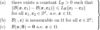 $$\begin{eqnarray}\left.\begin{array}{@{}ll@{}}\text{(a) } & \text{there exists a constant }L_{{\mathcal{B}}}>0\text{ such that}~\\ & \Vert {\mathcal{B}}(\boldsymbol{x},\unicode[STIX]{x1D73A}_{1})-{\mathcal{B}}(\boldsymbol{x},\unicode[STIX]{x1D73A}_{2})\Vert \leq L_{{\mathcal{B}}}\Vert \unicode[STIX]{x1D73A}_{1}-\unicode[STIX]{x1D73A}_{2}\Vert \\ & \text{for all }\unicode[STIX]{x1D73A}_{1},\unicode[STIX]{x1D73A}_{2}\in \mathbb{S}^{d},~\text{a.e.}~\boldsymbol{x}\in \unicode[STIX]{x1D6FA};\\[3.0pt] \text{(b) } & {\mathcal{B}}(\cdot ,\unicode[STIX]{x1D73A})\text{ is measurable on }\unicode[STIX]{x1D6FA}\text{ for all }\unicode[STIX]{x1D73A}\in \mathbb{S}^{d};\\[3.0pt] \text{(c) } & {\mathcal{B}}(\boldsymbol{x},\mathbf{0})=\mathbf{0}~\text{a.e.}~\boldsymbol{x}\in \unicode[STIX]{x1D6FA}.\end{array}\right\}\end{eqnarray}$$
For the normal potential function
 $j_{\unicode[STIX]{x1D708}}:\unicode[STIX]{x1D6E4}_{3}\times \mathbb{R}\rightarrow \mathbb{R}$
, we assume:
 $$\begin{eqnarray}\left.\begin{array}{@{}ll@{}}\text{(a) } & j_{\unicode[STIX]{x1D708}}(\cdot ,r)\text{ is measurable on }\unicode[STIX]{x1D6E4}_{3}\text{ for all }r\in \mathbb{R}\text{ and there}\\ & \text{exists }\bar{e}_{\unicode[STIX]{x1D708}}\in L^{2}(\unicode[STIX]{x1D6E4}_{3})\text{ such that }j_{\unicode[STIX]{x1D708}}(\cdot ,\bar{e}_{\unicode[STIX]{x1D708}}(\cdot ))\in L^{1}(\unicode[STIX]{x1D6E4}_{3});\\[3.0pt] \text{(b) } & j_{\unicode[STIX]{x1D708}}(\boldsymbol{x},\cdot )\text{ is locally Lipschitz on }\mathbb{R}\text{ for a.e. }\boldsymbol{x}\in \unicode[STIX]{x1D6E4}_{3};\\[3.0pt] \text{(c) } & |\unicode[STIX]{x2202}j_{\unicode[STIX]{x1D708}}(\boldsymbol{x},r)|\leq \bar{c}_{0\unicode[STIX]{x1D708}}\text{ for a.e. }\boldsymbol{x}\in \unicode[STIX]{x1D6E4}_{3},\text{ for }r\in \mathbb{R}\text{ with }\bar{c}_{0\unicode[STIX]{x1D708}}\geq 0;~\\[3.0pt] \text{(d) } & j_{\unicode[STIX]{x1D708}}^{0}(\boldsymbol{x},r_{1};r_{2}-r_{1})+j_{\unicode[STIX]{x1D708}}^{0}(\boldsymbol{x},r_{2};r_{1}-r_{2})\leq \unicode[STIX]{x1D6FC}_{j_{\unicode[STIX]{x1D708}}}|r_{1}-r_{2}|^{2}\\ & \text{for a.e. }\boldsymbol{x}\in \unicode[STIX]{x1D6E4}_{3},~\text{all}~r_{1},\,r_{2}\in \mathbb{R}\text{ with }\unicode[STIX]{x1D6FC}_{j_{\unicode[STIX]{x1D708}}}\geq 0.\end{array}\right\}\end{eqnarray}$$
For the tangential potential function
 $j_{\unicode[STIX]{x1D70F}}:\unicode[STIX]{x1D6E4}_{3}\times \mathbb{R}^{d}\rightarrow \mathbb{R}$
, we assume:
 $$\begin{eqnarray}\left.\begin{array}{@{}ll@{}}\text{(a) } & j_{\unicode[STIX]{x1D70F}}(\cdot ,\unicode[STIX]{x1D743})\text{ is measurable on }\unicode[STIX]{x1D6E4}_{3}\text{ for all }\unicode[STIX]{x1D743}\in \mathbb{R}^{d}\text{ and there}\\ & \text{exists }\bar{\boldsymbol{e}}_{\unicode[STIX]{x1D70F}}\in L^{2}(\unicode[STIX]{x1D6E4}_{3})^{d}\text{ such that }j_{\unicode[STIX]{x1D70F}}(\cdot ,\bar{\boldsymbol{e}}_{\unicode[STIX]{x1D70F}}(\cdot ))\in L^{1}(\unicode[STIX]{x1D6E4}_{3});\\[3.0pt] \text{(b) } & j_{\unicode[STIX]{x1D70F}}(\boldsymbol{x},\cdot )\text{ is locally Lipschitz on }\mathbb{R}^{d}\text{ for a.e.}~\boldsymbol{x}\in \unicode[STIX]{x1D6E4}_{3};\\[3.0pt] \text{(c) } & |\unicode[STIX]{x2202}j_{\unicode[STIX]{x1D70F}}(\boldsymbol{x},\unicode[STIX]{x1D743})|\leq \bar{c}_{0\unicode[STIX]{x1D70F}}\text{ for a.e. }\boldsymbol{x}\in \unicode[STIX]{x1D6E4}_{3},\text{for }\unicode[STIX]{x1D743}\in \mathbb{R}^{d}\text{ with }\bar{c}_{0\unicode[STIX]{x1D70F}}\geq 0;~\\[3.0pt] \text{(d) } & j_{\unicode[STIX]{x1D70F}}^{0}(\boldsymbol{x},\unicode[STIX]{x1D743}_{1};\unicode[STIX]{x1D743}_{2}-\unicode[STIX]{x1D743}_{1})+j_{\unicode[STIX]{x1D70F}}^{0}(\boldsymbol{x},\unicode[STIX]{x1D743}_{2};\unicode[STIX]{x1D743}_{1}-\unicode[STIX]{x1D743}_{2})\leq \unicode[STIX]{x1D6FC}_{j_{\unicode[STIX]{x1D70F}}}\Vert \unicode[STIX]{x1D743}_{1}-\unicode[STIX]{x1D743}_{2}\Vert ^{2}\\ & \text{for a.e.}~\boldsymbol{x}\in \unicode[STIX]{x1D6E4}_{3},\text{all }\unicode[STIX]{x1D743}_{1},\,\unicode[STIX]{x1D743}_{2}\in \mathbb{R}^{d}\text{ with }\unicode[STIX]{x1D6FC}_{j_{\unicode[STIX]{x1D70F}}}\geq 0.\end{array}\right\}\end{eqnarray}$$
For the mass density assume it is a positive constant,
 $$\begin{eqnarray}\unicode[STIX]{x1D70C}>0.\end{eqnarray}$$
For the densities of body forces and surface tractions, assume
 $$\begin{eqnarray}\boldsymbol{f}_{0}\in L^{2}(0,T;L^{2}(\unicode[STIX]{x1D6FA};\mathbb{R}^{d})),\quad \boldsymbol{f}_{2}\in L^{2}(0,T;L^{2}(\unicode[STIX]{x1D6E4}_{2};\mathbb{R}^{d})),\end{eqnarray}$$
and for the initial data,
 $$\begin{eqnarray}\boldsymbol{u}_{0}\in V,\quad \boldsymbol{w}_{0}\in H.\end{eqnarray}$$
Recall that the spaces
 $V$
and
 $H$
are defined by (2.3) and (2.5), respectively. Then, the weak formulation of Problem 2.9, obtained by using arguments similar to those used in Section 2.1, is as follows.
Problem 2.10. Find a displacement field
 $\boldsymbol{u}:[0,T]\rightarrow V$
such that
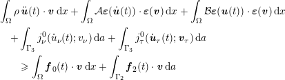 $$\begin{eqnarray}\displaystyle & & \displaystyle \int _{\unicode[STIX]{x1D6FA}}\unicode[STIX]{x1D70C}\,\ddot{\boldsymbol{u}}(t)\cdot \boldsymbol{v}\,\text{d}x+\int _{\unicode[STIX]{x1D6FA}}{\mathcal{A}}\unicode[STIX]{x1D73A}(\dot{\boldsymbol{u}}(t))\cdot \unicode[STIX]{x1D73A}(\boldsymbol{v})\,\text{d}x+\int _{\unicode[STIX]{x1D6FA}}{\mathcal{B}}\unicode[STIX]{x1D73A}(\boldsymbol{u}(t))\cdot \unicode[STIX]{x1D73A}(\boldsymbol{v})\,\text{d}x\nonumber\\ \displaystyle & & \displaystyle \quad +\int _{\unicode[STIX]{x1D6E4}_{3}}j_{\unicode[STIX]{x1D708}}^{0}(\dot{u}_{\unicode[STIX]{x1D708}}(t);v_{\unicode[STIX]{x1D708}})\,\text{d}a+\int _{\unicode[STIX]{x1D6E4}_{3}}j_{\unicode[STIX]{x1D70F}}^{0}(\dot{\boldsymbol{u}}_{\unicode[STIX]{x1D70F}}(t);\boldsymbol{v}_{\unicode[STIX]{x1D70F}})\,\text{d}a\nonumber\\ \displaystyle & & \displaystyle \quad \quad \geq \int _{\unicode[STIX]{x1D6FA}}\boldsymbol{f}_{0}(t)\cdot \boldsymbol{v}\,\text{d}x+\int _{\unicode[STIX]{x1D6E4}_{2}}\boldsymbol{f}_{2}(t)\cdot \boldsymbol{v}\,\text{d}a\end{eqnarray}$$
for all
 $\boldsymbol{v}\in V$
,
 $t\in [0,T]$
, and
 $$\begin{eqnarray}\boldsymbol{u}(0)=\boldsymbol{u}_{0},\quad \dot{\boldsymbol{u}}(0)=\boldsymbol{w}_{0}.\end{eqnarray}$$
Note that inequality (2.71) involves the second time derivative of the unknown function
 $\boldsymbol{u}$
. Consequently, the initial conditions (2.72) are introduced. We refer to such an inequality as an evolutionary hemivariational inequality. The well-posedness analysis and numerical approximations of Problem 2.6 will be provided in Section 9.
3 Preliminaries
As shown in the previous section, the weak formulations of contact problems lead to hemivariational or variational–hemivariational inequalities in which the unknown is the displacement field. In this section we present preliminary material needed to obtain an abstract existence and uniqueness result in the study of such inequalities. In this way we lay the background necessary in the well-posedness analysis and numerical approximation of the corresponding contact models. The preliminaries presented here include basic notions and results on non-smooth analysis, convex subdifferentials for convex functions, Clarke subdifferentials for locally Lipschitz functions, surjectivity for pseudomonotone multivalued operators, fixed-point theorems, and Gronwall inequalities. The material can be found in many textbooks and monographs. For this reason we present the theorems and propositions below without proofs and refer the reader to appropriate references.
Unless stated otherwise, in the rest of this section we assume
 $X$
is a real reflexive Banach space. We let
 $\Vert \cdot \Vert _{X}$
denote its norm,
 $X^{\ast }$
its topological dual, and
 $\langle \cdot ,\cdot \rangle$
the canonical duality pairing between
 $X^{\ast }$
and
 $X$
. Moreover,
 $2^{X^{\ast }}$
denotes the set of all subsets of
 $X^{\ast }$
and
 $X_{w^{\ast }}^{\ast }$
represents the space
 $X^{\ast }$
equipped with the weak
 $^{\,\ast }$
topology. Finally, we let
 ${\mathcal{L}}(X,Y)$
denote the space of linear continuous operators defined on
 $X$
with values in the normed space
 $Y$
, equipped with the canonical norm
 $\Vert \cdot \Vert _{{\mathcal{L}}(X,Y)}$
.
3.1 Basics on non-smooth analysis
Nonlinear operators of monotone type.
We start with some definitions concerning single-valued operators.
Definition 3.1. An operator
 $A:X\rightarrow X^{\ast }$
is called:
(a) bounded if
 $A$
maps bounded sets of
$X$
into bounded sets of
$X^{\ast }$
;
(b) hemicontinuous if, for all
$u,v,w\in X$
, the function
$t\mapsto \langle A(u+t\,v),w\rangle$
is continuous for
$t\in [0,1]$
;(c) monotone if
$\langle Au-Av,u-v\rangle \geq 0$
for all
$u$
,
$v\in X$
;(d) maximal monotone if it is monotone and
$\langle w-Av,u-v\rangle \geq 0$
for any
$v\in X$
implies that
$w=Au$
;(e)
$u_{0}$
-coercive if there exists a function
$\unicode[STIX]{x1D6FC}:\mathbb{R}_{+}\rightarrow \mathbb{R}$
with
$\lim _{r\rightarrow +\infty }\unicode[STIX]{x1D6FC}(r)=+\infty$
such that
$\langle Au,u-u_{0}\rangle \geq \unicode[STIX]{x1D6FC}(\Vert u\Vert _{X})\,\Vert u\Vert _{X}$
for all
$u\in X$
, where
$u_{0}$
is a given element in
$X$
;(f) pseudomonotone if it is bounded and
$u_{n}\rightarrow u$
weakly in
$X$
with
$\displaystyle \limsup \,\langle Au_{n},u_{n}-u\rangle \leq 0$
imply
$\displaystyle \liminf \,\langle Au_{n},u_{n}-v\rangle \geq \langle Au,u-v\rangle$
for all
$v\in X$
;(g) radially continuous if, for any
$u,v\in X$
, the function
$t\mapsto \langle A(u+t\,v),v\rangle$
is continuous on
$[0,1]$
.




















Remark 3.2. It can be proved that an operator
 $A:X\rightarrow X^{\ast }$
is pseudomonotone if and only if it is bounded and
 $u_{n}\rightarrow u$
weakly in
 $X$
together with
 $\displaystyle \limsup \,\langle Au_{n},u_{n}-u\rangle \leq 0$
imply
 $\displaystyle \lim \,\langle Au_{n},u_{n}-u\rangle =0$
and
 $Au_{n}\rightarrow Au$
weakly in
 $X^{\ast }$
.
 $\Box$
We note that if
 $A:X\rightarrow X^{\ast }$
is continuous, then it is hemicontinuous. The following result can be deduced from Zeidler (Reference Zeidler1990, Proposition 27.6).
Proposition 3.3. If
 $A:X\rightarrow X^{\ast }$
is bounded, hemicontinuous and monotone, then it is pseudomonotone.
Next, we move to multivalued operators defined on the space
 $X$
. Given a multivalued operator
 $T:X\rightarrow 2^{X^{\ast }}$
, its domain
 ${\mathcal{D}}(T)$
, range
 ${\mathcal{R}}(T)$
and graph
 ${\mathcal{G}}(T)$
are the sets defined by
 $$\begin{eqnarray}\displaystyle {\mathcal{D}}(T) & = & \displaystyle \{x\in X\mid Tx\not =\emptyset \},\nonumber\\ \displaystyle {\mathcal{R}}(T) & = & \displaystyle \bigcup \,\{Tx\mid x\in X\},\nonumber\\ \displaystyle {\mathcal{G}}(T) & = & \displaystyle \{(x,x^{\ast })\in X\times X^{\ast }\mid x^{\ast }\in Tx\},\nonumber\end{eqnarray}$$
respectively. We proceed with the following definitions.
Definition 3.4. An operator
 $T:X\rightarrow 2^{X^{\ast }}$
is called:
(a) bounded if the range of any bounded set in
$X$
is a bounded set in
$X^{\ast }$
;(b) monotone if
$\langle u^{\ast }-v^{\ast },u-v\rangle \geq 0$
for all
$(u,u^{\ast })$
,
$(v,v^{\ast })\in {\mathcal{G}}(T)$
;(c) maximal monotone if it is monotone and maximal in the sense of inclusion of graphs in the family of monotone operators from
$X$
to
$2^{X^{\ast }}$
;(d)
$u_{0}$
-coercive if there exists a function
$\unicode[STIX]{x1D6FC}:\mathbb{R}_{+}\rightarrow \mathbb{R}$
with
$\lim _{r\rightarrow +\infty }\unicode[STIX]{x1D6FC}(r)=+\infty$
such that for all
$(u,u^{\ast })\in {\mathcal{G}}(T)$
we have where$$\begin{eqnarray}\langle u^{\ast },u-u_{0}\rangle \geq \unicode[STIX]{x1D6FC}(\Vert u\Vert _{X})\,\Vert u\Vert _{X},\end{eqnarray}$$
$u_{0}$
is a given element in
$X$
;(e) generalized pseudomonotone if, for any sequences
$\{u_{n}\}\!\subset \!X$
and
$\{u_{n}^{\ast }\}\!\subset \!X^{\ast }$
such that
$u_{n}\rightarrow u$
weakly in
$X$
,
$u_{n}^{\ast }\in Tu_{n}$
for all
$n\in \mathbb{N}$
,
$u_{n}^{\ast }\rightarrow u^{\ast }$
weakly in
$X^{\ast }$
and
$\limsup \,\langle u_{n}^{\ast },u_{n}-u\rangle \leq 0$
, we have
$u^{\ast }\in Tu$
and $$\begin{eqnarray}\lim \,\langle u_{n}^{\ast },u_{n}\rangle =\langle u^{\ast },u\rangle .\end{eqnarray}$$











Given
 $u_{0}\in X$
and
 $T:X\rightarrow 2^{X^{\ast }}$
, we define a multivalued operator
 $T_{u_{0}}$
by
 $T_{u_{0}}(v)=T(v+u_{0})$
for
 $v\in X$
. The following surjectivity result concerns the sum of a generalized pseudomonotone operator and a maximal monotone one. Its proof can be found in Naniewicz and Panagiotopoulos (Reference Naniewicz and Panagiotopoulos1995).
Theorem 3.5. Let
 $X$
be a reflexive Banach space,
 $T_{1}:X\rightarrow 2^{X^{\ast }}$
,
 $T_{2}:X\rightarrow 2^{X^{\ast }}$
and
 $u_{0}\in X$
. Assume
(a)
$T_{1}$
is bounded, generalized pseudomonotone and
$u_{0}$
-coercive;(b)
$T_{1}u$
is a non-empty, closed and convex subset of
$X^{\ast }$
, for all
$u\in X$
;(c)
$T_{2}$
is a maximal monotone operator, and
$u_{0}\in {\mathcal{D}}(T_{2})$
.


Then
 $T_{1}+T_{2}:X\rightarrow 2^{X^{\ast }}$
is surjective, i.e.
 ${\mathcal{R}}(T_{1}+T_{2})=X^{\ast }$
.
Theorem 3.5 will be employed in the proof of the solvability of elliptic variational–hemivariational inequalities on the space
 $X$
.
Convex functions.
Let
 $\unicode[STIX]{x1D711}:X\rightarrow \mathbb{R}\cup \{+\infty \}$
. The effective domain of
 $\unicode[STIX]{x1D711}$
is the set
 $\text{dom}\,\unicode[STIX]{x1D711}=\{x\in X\mid \unicode[STIX]{x1D711}(x)<+\infty \}$
. We say that
 $\unicode[STIX]{x1D711}$
is convex if, for all
 $x$
,
 $y\in \text{dom}\,\unicode[STIX]{x1D711}$
and all
 $\unicode[STIX]{x1D706}\in (0,1)$
, we have
 $$\begin{eqnarray}\unicode[STIX]{x1D711}(\unicode[STIX]{x1D706}x+(1-\unicode[STIX]{x1D706})y)\leq \unicode[STIX]{x1D706}\unicode[STIX]{x1D711}(x)+(1-\unicode[STIX]{x1D706})\unicode[STIX]{x1D711}(y).\end{eqnarray}$$
The function
 $\unicode[STIX]{x1D711}$
is said to be proper if
 $\text{dom}\,\unicode[STIX]{x1D711}\not =\emptyset$
. The function
 $\unicode[STIX]{x1D711}:X\rightarrow \mathbb{R}\cup \{+\infty \}$
is lower semicontinuous (l.s.c.) if, for any
 $u\in X$
and for any sequence
 $\{u_{n}\}\subset X$
such that
 $u_{n}\rightarrow u$
in
 $X$
, we have
 $$\begin{eqnarray}\liminf \unicode[STIX]{x1D711}(u_{n})\geq \unicode[STIX]{x1D711}(u).\end{eqnarray}$$
Next, we recall the notion of the subdifferential of a convex function.
Definition 3.6. Let
 $\unicode[STIX]{x1D711}:X\rightarrow \mathbb{R}\cup \{+\infty \}$
be a proper and convex function. The mapping
 $\unicode[STIX]{x2202}_{c}\unicode[STIX]{x1D711}:X\rightarrow 2^{X^{\ast }}$
defined by
 $$\begin{eqnarray}\unicode[STIX]{x2202}_{c}\unicode[STIX]{x1D711}(x)=\{x^{\ast }\in X^{\ast }\mid \langle x^{\ast },v-x\rangle \leq \unicode[STIX]{x1D711}(v)-\unicode[STIX]{x1D711}(x)~\text{for all}~v\in X\}\end{eqnarray}$$
is called the convex subdifferential of
 $\unicode[STIX]{x1D711}$
. If
 $\unicode[STIX]{x2202}_{c}\unicode[STIX]{x1D711}(x)$
is non-empty, any element
 $x^{\ast }\in \unicode[STIX]{x2202}_{c}\unicode[STIX]{x1D711}(x)$
is called a subgradient of
 $\unicode[STIX]{x1D711}$
at
 $x$
.
It is easy to see that
 $\unicode[STIX]{x2202}_{c}\unicode[STIX]{x1D711}:X\rightarrow 2^{X^{\ast }}$
is a monotone operator. Moreover, we have the following well-known result.
Theorem 3.7. Let
 $X$
be a Banach space and
 $\unicode[STIX]{x1D711}:X\rightarrow \mathbb{R}\cup \{+\infty \}$
a proper, convex, l.s.c. function. Then
 $\unicode[STIX]{x2202}_{c}\unicode[STIX]{x1D711}:X\rightarrow 2^{X^{\ast }}$
is maximal monotone.
A proof of Theorem 3.7 can be found in Denkowski, Migórski and Papageorgiou (Reference Denkowski, Migórski and Papageorgiou2003b ).
In many situations we deal with functions
 $\unicode[STIX]{x1D711}:K\rightarrow \mathbb{R}$
where
 $K$
is a non-empty subset of
 $X$
. In such cases it is convenient to extend the function
 $\unicode[STIX]{x1D711}$
to the space
 $X$
by considering the function
 $\widetilde{\unicode[STIX]{x1D711}}:X\rightarrow \mathbb{R}\cup \{+\infty \}$
defined by
 $$\begin{eqnarray}\widetilde{\unicode[STIX]{x1D711}}(v)=\left\{\begin{array}{@{}ll@{}}\unicode[STIX]{x1D711}(v)\quad & \text{if }v\in K,\\ +\infty \quad & \text{otherwise.}\end{array}\right.\end{eqnarray}$$
We say that the function
 $\unicode[STIX]{x1D711}:K\rightarrow \mathbb{R}$
is convex if its extension
 $\widetilde{\unicode[STIX]{x1D711}}:X\rightarrow \mathbb{R}\cup \{+\infty \}$
is convex. It is lower semicontinuous (on
 $K$
) if
 $\widetilde{\unicode[STIX]{x1D711}}$
is lower semicontinuous. The special case
 $\unicode[STIX]{x1D711}=0$
deserves a more detailed treatment.
Example 3.8. Given a non-empty subset
 $K$
of
 $X$
, the function
 $I_{K}$
on
 $X$
, defined by
 $$\begin{eqnarray}I_{K}(x)=\left\{\begin{array}{@{}ll@{}}0\quad & \text{if}~x\in K,\\ +\infty \quad & \text{if}~x\notin K,\end{array}\right.\end{eqnarray}$$
is called the indicator function of
 $K$
. It can be proved that the subset
 $K$
of
 $X$
is convex if and only if
 $I_{K}$
is convex. Moreover,
 $K$
is closed if and only if
 $I_{K}$
is l.s.c. The subdifferential of
 $I_{K}$
is the multivalued operator
 $\unicode[STIX]{x2202}_{c}I_{K}:X\rightarrow 2^{X^{\ast }}$
given by
 $$\begin{eqnarray}\unicode[STIX]{x2202}_{c}I_{K}(x)=\left\{\begin{array}{@{}ll@{}}\{x^{\ast }\in X^{\ast }\mid \langle x^{\ast },x-v\rangle \geq 0~\,\text{for all}~v\in K\}\quad & \text{if}~x\in K,\\ \emptyset \quad & \text{if}~x\notin K.\end{array}\right.\end{eqnarray}$$
It follows from (3.1) that
 $$\begin{eqnarray}x^{\ast }\in \unicode[STIX]{x2202}_{c}I_{K}(x)\quad \Longleftrightarrow \quad x\in K,\quad \langle x^{\ast },x-v\rangle \geq 0\quad \text{for all}~v\in K.\end{eqnarray}$$
For detailed discussion of the properties of the convex functions, including the convex subdifferential, we refer the reader to Ekeland and Temam (Reference Ekeland and Temam1976) and Kurdila and Zabarankin (Reference Kurdila and Zabarankin2005), for instance.
Clarke subdifferential.
We now review the notion of the Clarke subdifferential for a locally Lipschitz function. First, we recall that a function
 $j:X\rightarrow \mathbb{R}$
is said to be locally Lipschitz if, for every
 $x\in X$
, there exists a neighbourhood of
 $x$
, denoted by
 $U_{x}$
, and a
 $U_{x}$
-dependent constant
 $L_{x}>0$
such that
 $$\begin{eqnarray}|j(y)-j(z)|\leq L_{x}\Vert y-z\Vert _{X}\quad \text{for all}~y,z\in U_{x}.\end{eqnarray}$$
We also recall that a convex continuous function
 $j:X\rightarrow \mathbb{R}$
is locally Lipschitz.
Definition 3.9. Let
 $j:X\rightarrow \mathbb{R}$
be a locally Lipschitz function. The generalized (Clarke) directional derivative of
 $j$
at a point
 $x\in X$
in a direction
 $v\in X$
is defined by
 $$\begin{eqnarray}j^{0}(x;v)=\limsup _{y\rightarrow x,\,\unicode[STIX]{x1D706}\downarrow 0}\displaystyle \frac{j(y+\unicode[STIX]{x1D706}v)-j(y)}{\unicode[STIX]{x1D706}}.\end{eqnarray}$$
The generalized gradient (subdifferential) of
 $j$
at
 $x$
is a subset of the dual space
 $X^{\ast }$
given by
 $$\begin{eqnarray}\unicode[STIX]{x2202}j(x)=\{\unicode[STIX]{x1D709}\in X^{\ast }\mid j^{0}(x;v)\geq \langle \unicode[STIX]{x1D709},v\rangle ~\text{for all}~v\in X\}.\end{eqnarray}$$
A locally Lipschitz function
 $j$
is said to be regular (in the sense of Clarke) at the point
 $x\in X$
if, for all
 $v\in X$
, the one-sided directional derivative
 $j^{\prime }(x;v)$
exists and
 $j^{0}(x;v)=j^{\prime }(x;v)$
.
We now follow Clarke (Reference Clarke1983) and recall the following properties of the generalized directional derivative and the generalized gradient.
Proposition 3.10. Assume that
 $j:X\rightarrow \mathbb{R}$
is a locally Lipschitz function. Then the following statements are valid.
(i) For every
$x\in X$
, the function
$X\ni v\mapsto j^{0}(x;v)\in \mathbb{R}$
is positively homogeneous and subadditive, that is,
$j^{0}(x;\unicode[STIX]{x1D706}v)=\unicode[STIX]{x1D706}j^{0}(x;v)$
for all
$\unicode[STIX]{x1D706}\geq 0$
,
$v\in X$
and
$j^{0}(x;v_{1}+v_{2})\leq j^{0}(x;v_{1})+j^{0}(x;v_{2})$
for all
$v_{1}$
,
$v_{2}\in X$
, respectively.(ii) For every
$v\in X$
, we have
$j^{0}(x;v)=\max \{\langle \unicode[STIX]{x1D709},v\rangle \mid \unicode[STIX]{x1D709}\in \unicode[STIX]{x2202}j(x)\}$
.(iii) The function
$X\times X\ni (x,v)\mapsto j^{0}(x;v)\in \mathbb{R}$
is upper semicontinuous, that is, for all
$x$
,
$v\in X$
,
$\{x_{n}\}$
,
$\{v_{n}\}\subset X$
such that
$x_{n}\rightarrow x$
and
$v_{n}\rightarrow v$
in
$X$
, we have
$\limsup j^{0}(x_{n};v_{n})\leq j^{0}(x;v)$
.(iv) For every
$x\in X$
, the generalized gradient
$\unicode[STIX]{x2202}j(x)$
is a non-empty, convex, and weakly
$^{\,\ast }$
compact subset of
$X^{\ast }$
.(v) The graph of the generalized gradient
$\unicode[STIX]{x2202}j$
is closed in
$X\times X_{w^{\ast }}^{\ast }$
topology, that is, if
$\{x_{n}\}\subset X$
and
$\{\unicode[STIX]{x1D709}_{n}\}\subset X^{\ast }$
are sequences such that
$\unicode[STIX]{x1D709}_{n}\in \unicode[STIX]{x2202}j(x_{n})$
and
$x_{n}\rightarrow x$
in
$X$
,
$\unicode[STIX]{x1D709}_{n}\rightarrow \unicode[STIX]{x1D709}$
weakly
$^{\ast }$
in
$X^{\ast }$
, then
$\unicode[STIX]{x1D709}\in \unicode[STIX]{x2202}j(x)$
.(vi) If
$j:X\rightarrow \mathbb{R}$
is convex, then the subdifferential in the sense of Clarke
$\unicode[STIX]{x2202}j(x)$
at any
$x\in X$
coincides with the convex subdifferential
$\unicode[STIX]{x2202}_{c}j(x)$
.















Proposition 3.11. Let
 $j,j_{1},j_{2}:X\rightarrow \mathbb{R}$
be locally Lipschitz functions. Then we have the following.
(i) Scalar multiples. The equality
$\unicode[STIX]{x2202}(\unicode[STIX]{x1D706}j)(x)=\unicode[STIX]{x1D706}\unicode[STIX]{x2202}j(x)$
holds for all
$\unicode[STIX]{x1D706}\in \mathbb{R}$
and all
$x\in X$
.(ii) Sum rules. The inclusion
(3.5)holds for all$$\begin{eqnarray}\unicode[STIX]{x2202}(j_{1}+j_{2})(x)\subseteq \unicode[STIX]{x2202}j_{1}(x)+\unicode[STIX]{x2202}j_{2}(x)\end{eqnarray}$$
$x\in X$
or, equivalently, (3.6)for all$$\begin{eqnarray}(j_{1}+j_{2})^{0}(x;v)\leq j_{1}^{0}(x;v)+j_{2}^{0}(x;v)~~\end{eqnarray}$$
$x\in X$
,
$v\in X$
.(iii) If
$j_{1}$
,
$j_{2}$
are regular at
$x\in X$
, then
$j_{1}+j_{2}$
is regular at
$x\in X$
and we have equalities in (3.5) and (3.6).






A proof of the following result can be found in Lemma 4.2 of Migórski, Ochal and Sofonea (Reference Migórski, Ochal and Sofonea2010) and follows from the chain rule for the generalized gradient.
Proposition 3.12. Let
 $X$
and
 $Y$
be Banach spaces, let
 $\unicode[STIX]{x1D711}:Y\rightarrow \mathbb{R}$
be locally Lipschitz and let
 $T:X\rightarrow Y$
be given by
 $Tx=Ax+y$
for
 $x\in X$
, where
 $A\in {\mathcal{L}}(X,Y)$
and
 $y\in Y$
is fixed. Then the function
 $j:X\rightarrow \mathbb{R}$
defined by
 $j(x)=\unicode[STIX]{x1D711}(Tx)$
is locally Lipschitz and
(i)
$j^{0}(x;v)\leq \unicode[STIX]{x1D711}^{0}(Tx;Av)$
for all
$x$
,
$v\in X$
,(ii)
$\unicode[STIX]{x2202}j(x)\subseteq A^{\ast }\unicode[STIX]{x2202}\unicode[STIX]{x1D711}(Tx)$
for all
$x\in X$
,





where
 $A^{\ast }\in {\mathcal{L}}(Y^{\ast },X^{\ast })$
is the adjoint operator of
 $A$
. Moreover, if
 $\unicode[STIX]{x1D711}$
(or
 $-\unicode[STIX]{x1D711}$
) is regular, then
 $j$
(or
 $-j$
) is regular and in (i) and (ii) we have equalities. These equalities are also true if instead of the regularity condition, we assume that
 $A$
is surjective.
For detailed discussion of the properties of the Clarke subdifferential, we refer the reader to Clarke (Reference Clarke1975, Reference Clarke1983) and Denkowski, Migórski and Papageorgiou (Reference Denkowski, Migórski and Papageorgiou2003a , Reference Denkowski, Migórski and Papageorgiou2003b ).
3.2 History-dependent operators
In the study of Problems 2.8 and 2.10, we will use the notion of a history-dependent operator. In contact mechanics, a history-dependent operator appears either in the constitutive law or in the contact boundary conditions. Such operators describe various memory effects. Abstract classes of quasivariational inequalities with history-dependent operators were considered in Sofonea and Matei (Reference Sofonea and Matei2011) and Sofonea and Xiao (Reference Sofonea and Xiao2016), where existence, uniqueness and regularity results were proved. A survey of some recent results for history-dependent variational–hemivariational inequalities can be found in Sofonea and Migórski (Reference Sofonea and Migórski2018). There, the abstract well-posedness results are applied to various examples arising in contact mechanics. In this subsection we assume that
 $X$
and
 $Y$
are normed spaces endowed with the norms
 $\Vert \cdot \Vert _{X}$
and
 $\Vert \cdot \Vert _{Y}$
, respectively. Let
 $I=[0,T]$
for some
 $T>0$
or
 $I=\mathbb{R}_{+}$
be the time interval of interest.
Definition 3.13. An operator
 ${\mathcal{S}}:C(I;X)\rightarrow C(I;Y)$
is called a history-dependent operator if, for any compact subset
 $I_{0}\subset I$
, there exists a constant
 $L_{I_{0}}>0$
such that
 $$\begin{eqnarray}\displaystyle \Vert {\mathcal{S}}u_{1}(t)-{\mathcal{S}}u_{2}(t)\Vert _{Y} & \leq & \displaystyle L_{I_{0}}\int _{0}^{t}\Vert u_{1}(s)-u_{2}(s)\Vert _{X}\,\text{d}s\nonumber\\ \displaystyle & & \displaystyle \qquad \text{for all}~u_{1},u_{2}\in C(I;X),\,t\in I_{0}.\end{eqnarray}$$
Similarly, an operator
 ${\mathcal{S}}:L^{2}(I;X)\rightarrow L^{2}(I;Y)$
is called a history-dependent operator if, for any compact subset
 $I_{0}\subset I$
, there exists a constant
 $L_{I_{0}}>0$
such that
 $$\begin{eqnarray}\displaystyle \Vert {\mathcal{S}}u_{1}(t)-{\mathcal{S}}u_{2}(t)\Vert _{Y} & \leq & \displaystyle L_{I_{0}}\int _{0}^{t}\Vert u_{1}(s)-u_{2}(s)\Vert _{X}\,\text{d}s\nonumber\\ \displaystyle & & \displaystyle \qquad \text{for all}~u_{1},u_{2}\in L^{2}(I;X),\text{ a.e. }t\in I_{0}.\end{eqnarray}$$
Note that here and below, when no confusion arises, we use the shorthand notation
 ${\mathcal{S}}u(t)$
to represent the value of the function
 ${\mathcal{S}}u$
at a point
 $t\in I$
, i.e.
 ${\mathcal{S}}u(t)=({\mathcal{S}}u)(t)$
. We make some comments regarding Definition 3.13 for
 ${\mathcal{S}}:C(I;X)\rightarrow C(I;Y)$
; similar comments can be stated for
 ${\mathcal{S}}:L^{2}(I;X)\rightarrow L^{2}(I;Y)$
.
Remark 3.14.
(1) An operator
${\mathcal{S}}:C([0,T];X)\rightarrow C([0,T];Y)$
is a history-dependent operator if and only if there exists a constant
$L>0$
such that (3.9)$$\begin{eqnarray}\displaystyle \Vert {\mathcal{S}}u_{1}(t)-{\mathcal{S}}u_{2}(t)\Vert _{Y} & \leq & \displaystyle L\int _{0}^{t}\Vert u_{1}(s)-u_{2}(s)\Vert _{X}\,\text{d}s\nonumber\\ \displaystyle & & \displaystyle \qquad \text{for all}~u_{1},u_{2}\in C([0,T];X),\,t\in [0,T].\end{eqnarray}$$
(2) An operator
${\mathcal{S}}:C(\mathbb{R}_{+};X)\rightarrow C(\mathbb{R}_{+};Y)$
is a history-dependent operator if and only if, for any
$n\in \mathbb{N}$
, there exists a constant
$L_{n}>0$
that varies with
$n$
, such that (3.10)$$\begin{eqnarray}\displaystyle \Vert {\mathcal{S}}u_{1}(t)-{\mathcal{S}}u_{2}(t)\Vert _{Y} & \leq & \displaystyle L_{n}\int _{0}^{t}\Vert u_{1}(s)-u_{2}(s)\Vert _{X}\,\text{d}s\nonumber\\ \displaystyle & & \displaystyle \qquad \text{for all}~u_{1},u_{2}\in C(\mathbb{R}_{+};X),\,t\in [0,n].\end{eqnarray}$$






Examples of operators satisfying condition (3.7) are given next.
Example 3.15. Let
 $u_{0}\in X$
and
 $G:X\rightarrow Y$
be a Lipschitz continuous operator, that is, an operator which satisfies the inequality
 $$\begin{eqnarray}\Vert Gu_{1}-Gu_{2}\Vert _{Y}\leq L_{G}\Vert u_{1}-u_{2}\Vert _{X}\quad \text{for all}~u_{1},u_{2}\in X\end{eqnarray}$$
with some constant
 $L_{G}>0$
. Define an operator
 ${\mathcal{S}}:C(I;X)\rightarrow C(I;Y)$
by
 $$\begin{eqnarray}{\mathcal{S}}u(t)=G\biggl(\int _{0}^{t}\,u(s)\,\text{d}s+u_{0}\biggr)\quad \text{for all}~u\in C(I;X),\,t\in I.\end{eqnarray}$$
Then, for
 $u_{1},u_{2}\in C(I;X)$
, we have
 $$\begin{eqnarray}\Vert {\mathcal{S}}u_{1}(t)-{\mathcal{S}}u_{2}(t)\Vert _{Y}\leq L_{G}\int _{0}^{t}\Vert u_{1}(s)-u_{2}(s)\Vert _{X}\,\text{d}s.\end{eqnarray}$$
Thus, condition (3.7) holds with
 $L_{I_{0}}=L_{G}$
for any compact subset
 $I_{0}\subset I$
and
 ${\mathcal{S}}$
is a history-dependent operator. In particular when
 $X=Y$
and
 $G$
is the identity operator on
 $X$
, (3.11) reduces to
 $$\begin{eqnarray}{\mathcal{S}}u(t)=\int _{0}^{t}u(s)\,\text{d}s+u_{0}\quad \text{for all}~u\in C(I;X),\,t\in I.\end{eqnarray}$$
The operator
 ${\mathcal{S}}:\!C(I;X)\rightarrow C(I;X)$
defined by (3.12) is a history-dependent operator.
Example 3.16. Let
 $G\in C(I;{\mathcal{L}}(X,Y))$
and
 ${\mathcal{S}}:C(I;X)\rightarrow C(I;Y)$
be a Volterra operator given by
 $$\begin{eqnarray}{\mathcal{S}}u(t)=\int _{0}^{t}G(t-s)\,u(s)\,\text{d}s,\quad u\in C(I;X),\,t\in I.\end{eqnarray}$$
Then for any compact set
 $I_{0}\subset I$
, inequality (3.7) holds with
 $$\begin{eqnarray}L_{I_{0}}=\Vert G\Vert _{C(I_{0};{\mathcal{L}}(X,Y))}=\max _{s\in I_{0}}\Vert G(s)\Vert _{{\mathcal{L}}(X,Y)}.\end{eqnarray}$$
This shows that the operator
 ${\mathcal{S}}$
defined by (3.13) is a history-dependent operator.
3.3 A class of evolutionary inclusions
We now introduce an abstract result which will be used in the study of the dynamic Problem 2.10. The functional framework is as follows. Let
 $V\subset H\subset V^{\ast }$
be an evolution triple of spaces, that is,
 $V$
is a separable, reflexive Banach space,
 $H$
is a separable Hilbert space, the embedding
 $V\subset H$
is continuous and
 $V$
is dense in
 $H$
. We use
 $\langle \cdot ,\cdot \rangle$
for the duality pairing between
 $V^{\ast }$
and
 $V$
. Given
 $0<T<+\infty$
, we introduce the function spaces
 $$\begin{eqnarray}{\mathcal{V}}=L^{2}(0,T;V)\quad \text{and}\quad {\mathcal{W}}=\{w\in {\mathcal{V}}\mid {\dot{w}}\in {\mathcal{V}}^{\ast }\}.\end{eqnarray}$$
We identify
 ${\mathcal{H}}=L^{2}(0,T;H)$
with its dual to obtain the following continuous embeddings
 ${\mathcal{W}}\subset {\mathcal{V}}\subset {\mathcal{H}}\subset {\mathcal{V}}^{\ast }$
. The duality pairing between
 ${\mathcal{V}}^{\ast }$
and
 ${\mathcal{V}}$
is denoted by
 $$\begin{eqnarray}\langle w,v\rangle _{{\mathcal{V}}^{\ast }\times {\mathcal{V}}}=\int _{0}^{T}\langle w(t),v(t)\rangle \,\text{d}t\quad \text{for}~w\in {\mathcal{V}}^{\ast },\,v\in {\mathcal{V}}.\end{eqnarray}$$
Now consider an operator
 $A:(0,T)\times V\rightarrow V^{\ast }$
and a function
 $\unicode[STIX]{x1D713}:(0,T)\times V\rightarrow \mathbb{R}$
, assumed to be locally Lipschitz with respect to its second argument. We let
 $\unicode[STIX]{x2202}\unicode[STIX]{x1D713}$
denote the Clarke generalized gradient of
 $\unicode[STIX]{x1D713}$
with respect to its second argument. Given
 $f:(0,T)\rightarrow V^{\ast }$
and
 $w_{0}\in V$
, we consider the following evolutionary inclusion.
Problem 3.17. Find
 $w\in {\mathcal{W}}$
such that
 $$\begin{eqnarray}\displaystyle & & \displaystyle {\dot{w}}(t)+A(t,w(t))+\unicode[STIX]{x2202}\unicode[STIX]{x1D713}(t,w(t))\ni f(t)~\text{for a.e.}~t\in (0,T),\nonumber\\ \displaystyle & & \displaystyle w(0)=w_{0}.\nonumber\end{eqnarray}$$
In the study of this inclusion problem, we impose the following hypotheses on the data.
 $$\begin{eqnarray}\displaystyle & & \displaystyle \left.\begin{array}{@{}ll@{}}A: & (0,T)\times V\rightarrow V^{\ast }\text{is such that:}\\[3.0pt] \text{(a) } & A(\cdot ,v)\text{ is measurable on }(0,T)\text{ for all }v\in V;\\[3.0pt] \text{(b) } & A(t,\cdot )\text{ is demicontinuous on }V\text{ for a.e.}~t\in (0,T),\\ & \text{i.e.}~u_{n}\rightarrow u\text{ in }V\Longrightarrow Au_{n}\rightharpoonup Au\text{ in }V^{\ast };\\[3.0pt] \text{(c) } & \Vert A(t,v)\Vert _{V^{\ast }}\leq a_{0}(t)+a_{1}\Vert v\Vert _{V}\text{ for all }v\in V,\\ & \text{a.e.}~t\in (0,T)\text{ with }a_{0}\in L^{2}(0,T),a_{0}\geq 0\text{ and }a_{1}\geq 0;~\\[3.0pt] \text{(d) } & \text{there is a constant }m_{A}>0\text{ such that}\\ & \langle A(t,v_{1})-A(t,v_{2}),v_{1}-v_{2}\rangle \geq m_{A}\Vert v_{1}-v_{2}\Vert _{V}^{2}\\ & \text{for all }v_{1},v_{2}\in V,\text{a.e.}~t\in (0,T).\end{array}\right\}\end{eqnarray}$$
 $$\begin{eqnarray}\displaystyle & & \displaystyle \left.\begin{array}{@{}ll@{}}\unicode[STIX]{x1D713}: & (0,T)\times V\rightarrow \mathbb{R}\text{ is such that:}\\ \text{(a) } & \unicode[STIX]{x1D713}(\cdot ,v)\text{ is measurable on }(0,T)\text{ for all }v\in V;\\[3.0pt] \text{(b) } & \unicode[STIX]{x1D713}(t,\cdot )\text{ is locally Lipschitz on }V\text{ for a.e.}~t\in (0,T);\\[3.0pt] \text{(c) } & \Vert \unicode[STIX]{x2202}\unicode[STIX]{x1D713}(t,v)\Vert _{V^{\ast }}\leq c_{0}(t)+c_{1}\Vert v\Vert _{V}\text{ for all }v\in V,\\ & \text{a.e.}~t\in (0,T)\text{ with }c_{0}\in L^{2}(0,T),c_{0}\geq 0,c_{1}\geq 0;\\[3.0pt] \text{(d) } & \text{there exists a constant }m_{\unicode[STIX]{x1D713}}\geq 0\text{ such that}\\ & \langle z_{1}-z_{2},v_{1}-v_{2}\rangle \geq -m_{\unicode[STIX]{x1D713}}\Vert v_{1}-v_{2}\Vert _{V}^{2}\\ & \text{for all }z_{i}\in \unicode[STIX]{x2202}\unicode[STIX]{x1D713}(t,v_{i}),\,z_{i}\in V^{\ast },\,v_{i}\in V,\,i=1,2,\text{a.e.}~t\in (0,T).\end{array}\right\}\end{eqnarray}$$
 $$\begin{eqnarray}\displaystyle & & \displaystyle \,f\in {\mathcal{V}}^{\ast },~w_{0}\in V.\end{eqnarray}$$
 $$\begin{eqnarray}\displaystyle & & \displaystyle \max \,\{m_{\unicode[STIX]{x1D713}},2\sqrt{2}\,c_{1}\}<m_{A}.\end{eqnarray}$$
We say a function
 $w\in {\mathcal{W}}$
is a solution of Problem 3.17 if there exists
 $w^{\ast }\in {\mathcal{V}}^{\ast }$
such that
 $$\begin{eqnarray}\displaystyle & & \displaystyle {\dot{w}}(t)+A(t,w(t))+w^{\ast }(t)=f(t)~\text{for a.e.}~t\in (0,T),\nonumber\\ \displaystyle & & \displaystyle w^{\ast }(t)\in \unicode[STIX]{x2202}\unicode[STIX]{x1D713}(t,w(t))~\text{for a.e.}~t\in (0,T),\nonumber\\ \displaystyle & & \displaystyle w(0)=w_{0}.\nonumber\end{eqnarray}$$
We have the following existence and uniqueness result.
Theorem 3.18. Assume that (3.14)–(3.17) hold. Then Problem 3.17 has a unique solution
 $w\in {\mathcal{W}}$
.
A proof of Theorem 3.18 can be found in Sofonea and Migórski (Reference Sofonea and Migórski2018, p. 183). The existence part is based on a surjectivity result with maximal monotone operators in reflexive Banach spaces. The uniqueness part follows from standard arguments and is based on the smallness assumption (3.17).
3.4 Fixed-point theorems
We will apply Banach’s fixed-point theorem in solution existence proofs of various problems: see Zeidler (Reference Zeidler1985, Section 1.1) or Atkinson and Han (Reference Atkinson and Han2009, Section 5.1).
Theorem 3.19. Let
 $K$
be a non-empty closed set in a Banach space
 $X$
, and let
 $\unicode[STIX]{x1D6EC}:K\rightarrow K$
be a contractive mapping, that is, for some constant
 $\unicode[STIX]{x1D6FC}\in [0,1)$
,
 $$\begin{eqnarray}\Vert \unicode[STIX]{x1D6EC}u-\unicode[STIX]{x1D6EC}v\Vert _{X}\leq \unicode[STIX]{x1D6FC}\,\Vert u-v\Vert _{X}\quad \text{for all}~u,v\in K.\end{eqnarray}$$
Then
 $\unicode[STIX]{x1D6EC}:K\rightarrow K$
has a unique fixed point, that is, there exists a unique
 $u^{\ast }\in K$
such that
 $$\begin{eqnarray}\unicode[STIX]{x1D6EC}u^{\ast }=u^{\ast }.\end{eqnarray}$$
History-dependent operators have important fixed-point properties which are useful in proving the solvability of various classes of nonlinear equations and inequalities. The following result is proved in Sofonea, Avramescu and Matei (Reference Sofonea, Avramescu and Matei2008).
Theorem 3.20. Assume that
 $X$
is a Banach space and
 $\unicode[STIX]{x1D6EC}:C(I;X)\rightarrow C(I;X)$
is a history-dependent operator. Then
 $\unicode[STIX]{x1D6EC}$
has a unique fixed point, that is, there exists a unique element
 $\unicode[STIX]{x1D702}^{\ast }\in C(I;X)$
such that
 $\unicode[STIX]{x1D6EC}\unicode[STIX]{x1D702}^{\ast }=\unicode[STIX]{x1D702}^{\ast }$
.
In case of a history-dependent operator on
 $L^{2}(0,T;X)$
, we have a similar result from Sofonea and Migórski (Reference Sofonea and Migórski2018, Theorem 67).
Theorem 3.21. Assume that
 $X$
is a Banach space and
 $\unicode[STIX]{x1D6EC}:L^{2}(0,T;X)\rightarrow L^{2}(0,T;X)$
is a history-dependent operator. Then
 $\unicode[STIX]{x1D6EC}$
has a unique fixed point, that is, there exists a unique element
 $\unicode[STIX]{x1D702}^{\ast }\in L^{2}(0,T;X)$
such that
 $\unicode[STIX]{x1D6EC}\unicode[STIX]{x1D702}^{\ast }=\unicode[STIX]{x1D702}^{\ast }$
.
3.5 Some inequalities
We will use the modified Cauchy–Schwarz inequality
 $$\begin{eqnarray}a\,b\leq \unicode[STIX]{x1D716}\,a^{2}+c\,b^{2}\quad \text{for all}~a,b\in \mathbb{R},\end{eqnarray}$$
where
 $\unicode[STIX]{x1D716}>0$
is an arbitrary positive number and the constant
 $c>0$
depends on
 $\unicode[STIX]{x1D716}$
; indeed, we may simply take
 $c=1/(4\,\unicode[STIX]{x1D716})$
.
In the well-posedness analysis of contact problems, we will need the Gronwall inequality: see Han and Sofonea (Reference Han and Sofonea2002, Section 7.4).
Lemma 3.22. Let
 $a,\,b\in \mathbb{R}$
with
 $a<b$
and assume
 $f,g:[a,b]\rightarrow \mathbb{R}$
are continuous functions satisfying
 $$\begin{eqnarray}f(t)\leq g(t)+c\int _{a}^{t}f(s)\,\text{d}s\quad \text{for all}~t\in [a,b],\end{eqnarray}$$
where
 $c>0$
is a constant. Then
 $$\begin{eqnarray}f(t)\leq g(t)+c\int _{a}^{t}g(s)\,\text{e}^{c\,(t-s)}\,\text{d}s\quad \text{for all}~t\in [a,b].\end{eqnarray}$$
Moreover, if
 $g$
is non-decreasing, then
 $$\begin{eqnarray}f(t)\leq g(t)\,\text{e}^{c\,(t-a)}\quad \text{for all}~t\in [a,b].\end{eqnarray}$$
In error analysis for numerical solutions of the contact problems, we will need discrete versions of Gronwall’s inequality. For a fixed
 $T$
and a positive integer
 $N$
, let
 $k=T/N$
.
Lemma 3.23. Assume
 $\{g_{n}\}_{n=1}^{N}$
and
 $\{e_{n}\}_{n=1}^{N}$
are two sequences of non-negative numbers satisfying
 $$\begin{eqnarray}e_{n}\leq c\,g_{n}+c\,k\mathop{\sum }_{i=1}^{n-1}e_{i},\quad n=1,\ldots ,N,\end{eqnarray}$$
for a constant
 $c>0$
. Then, for a possibly different constant
 $c>0$
,
 $$\begin{eqnarray}\max _{1\leq n\leq N}e_{n}\leq c\,\max _{1\leq n\leq N}g_{n}.\end{eqnarray}$$
Lemma 3.24. Assume
 $\{g_{n}\}_{n=1}^{N}$
and
 $\{e_{n}\}_{n=1}^{N}$
are two sequences of non-negative numbers satisfying
 $$\begin{eqnarray}e_{n}\leq c\,g_{n}+c\,k\mathop{\sum }_{i=1}^{n}e_{i},\quad n=1,\ldots ,N,\end{eqnarray}$$
for a constant
 $c>0$
. Then, if
 $k$
is sufficiently small,
 $$\begin{eqnarray}\max _{1\leq n\leq N}e_{n}\leq c\,\max _{1\leq n\leq N}g_{n}.\end{eqnarray}$$
More general versions of these results can be found in Han and Sofonea (Reference Han and Sofonea2002, Section 7.4).
4 An elliptic variational–hemivariational inequality
In this section we consider an abstract elliptic variational–hemivariational inequality, present a well-posedness result, develop numerical methods for its solution, prove convergence of the numerical solutions, and provide a Céa-type inequality for error estimation of the numerical solutions. The results in this section will be applied in Section 7 in the analysis of Problem 2.6.
Let
 $X$
be a reflexive Banach space. Given a set
 $K\subset X$
, an operator
 $A:X\rightarrow X^{\ast }$
, functions
 $\unicode[STIX]{x1D711}:K\times K\rightarrow \mathbb{R}$
,
 $j:X\rightarrow \mathbb{R}$
and
 $f\in X^{\ast }$
, we consider the following problem.
Problem 4.1. Find an element
 $u\in K$
such that
 $$\begin{eqnarray}\langle Au,v-u\rangle +\unicode[STIX]{x1D711}(u,v)-\unicode[STIX]{x1D711}(u,u)+j^{0}(u;v-u)\geq \langle f,v-u\rangle \quad \text{for all}~v\in K.\end{eqnarray}$$
Note that Problem 4.1 contains a function
 $\unicode[STIX]{x1D711}$
assumed to be convex with respect to its second argument and a function
 $j$
assumed to be locally Lipschitz. Therefore, Problem 4.1 represents a variational–hemivariational inequality.
For the analysis of Problem 4.1, we consider the following hypotheses on the data.
 $$\begin{eqnarray}\displaystyle & & \displaystyle ~\,K\text{ is a non-empty, closed, convex subset of }X.\end{eqnarray}$$
 $$\begin{eqnarray}\displaystyle & & \displaystyle \left.\begin{array}{@{}ll@{}}A: & X\rightarrow X^{\ast }\text{is:}\\[3.0pt] \text{(a) } & \text{bounded and hemicontinuous};\\[3.0pt] \text{(b) } & \text{strongly monotone, i.e. for some constant }m_{A}>0,\\ & \langle Av_{1}-Av_{2},v_{1}-v_{2}\rangle \geq m_{A}\Vert v_{1}-v_{2}\Vert _{X}^{2}~\text{for all}~v_{1},v_{2}\in X.~\end{array}\right\}\end{eqnarray}$$
 $$\begin{eqnarray}\displaystyle & & \displaystyle \left.\begin{array}{@{}ll@{}}\unicode[STIX]{x1D711}: & K\times K\rightarrow \mathbb{R}\text{ is such that:}\\[3.0pt] \text{(a) } & \unicode[STIX]{x1D711}(\unicode[STIX]{x1D702},\cdot ):K\rightarrow \mathbb{R}\text{ is convex and l.s.c. on}K\text{ for all }\unicode[STIX]{x1D702}\in K;~\\[3.0pt] \text{(b) } & \text{there exists a constant }\unicode[STIX]{x1D6FC}_{\unicode[STIX]{x1D711}}>0\text{ such that}\\ & \unicode[STIX]{x1D711}(\unicode[STIX]{x1D702}_{1},v_{2})-\unicode[STIX]{x1D711}(\unicode[STIX]{x1D702}_{1},v_{1})+\unicode[STIX]{x1D711}(\unicode[STIX]{x1D702}_{2},v_{1})-\unicode[STIX]{x1D711}(\unicode[STIX]{x1D702}_{2},v_{2})\\ & \leq \unicode[STIX]{x1D6FC}_{\unicode[STIX]{x1D711}}\Vert \unicode[STIX]{x1D702}_{1}-\unicode[STIX]{x1D702}_{2}\Vert _{X}\Vert v_{1}-v_{2}\Vert _{X}~\text{for all}~\unicode[STIX]{x1D702}_{1},\unicode[STIX]{x1D702}_{2},v_{1},v_{2}\in K.\end{array}\right\}\end{eqnarray}$$
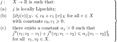 $$\begin{eqnarray}\displaystyle & & \displaystyle \left.\begin{array}{@{}ll@{}}j:\, & X\rightarrow \mathbb{R}\text{ is such that:}\\[3.0pt] \text{(a) } & j\text{ is locally Lipschitz;}\\[3.0pt] \text{(b) } & \Vert \unicode[STIX]{x2202}j(v)\Vert _{X^{\ast }}\leq c_{0}+c_{1}\,\Vert v\Vert _{X}\text{ for all }v\in X\\ & \text{with constants }c_{0},c_{1}\geq 0;\\[3.0pt] \text{(c) } & \text{there exists a constant }\unicode[STIX]{x1D6FC}_{j}>0\text{ such that}\\ & j^{0}(v_{1};v_{2}-v_{1})+j^{0}(v_{2};v_{1}-v_{2})\leq \unicode[STIX]{x1D6FC}_{j}\Vert v_{1}-v_{2}\Vert _{X}^{2}~\\ & \text{for all }~v_{1},v_{2}\in X.\end{array}\right\}\end{eqnarray}$$
 $$\begin{eqnarray}\displaystyle & & \displaystyle ~\,f\in X^{\ast }.\end{eqnarray}$$
Recall that, as usual, inequality in (4.4(b)) means
 $$\begin{eqnarray}\Vert \unicode[STIX]{x1D709}\Vert _{X^{\ast }}\leq c_{0}+c_{1}\,\Vert v\Vert _{X}\quad \text{for all}~v\in X,~\unicode[STIX]{x1D709}\in \unicode[STIX]{x2202}j(v).\end{eqnarray}$$
Moreover, we recall that (4.4(c)) is equivalent to the following condition:
 $$\begin{eqnarray}\langle \unicode[STIX]{x2202}j(v_{1})-\unicode[STIX]{x2202}j(v_{2}),v_{1}-v_{2}\rangle \geq -\unicode[STIX]{x1D6FC}_{j}\,\Vert v_{1}-v_{2}\Vert _{X}^{2}\quad \text{for all}~v_{1},v_{2}\in X.\end{eqnarray}$$
A proof of this statement can be found in Sofonea and Migórski (Reference Sofonea and Migórski2018, p. 124).
4.1 Solution existence and uniqueness
The unique solvability of Problem 4.1 is provided by the following result.
Theorem 4.2. Assume (4.1)–(4.5) and the smallness condition
 $$\begin{eqnarray}\unicode[STIX]{x1D6FC}_{\unicode[STIX]{x1D711}}+\unicode[STIX]{x1D6FC}_{j}<m_{A}.\end{eqnarray}$$
Then, Problem 4.1 has a unique solution
 $u\in K$
.
A version of Theorem 4.2 was proved in Migórski, Ochal and Sofonea (Reference Migórski, Ochal and Sofonea2017), under additional assumptions. The proof of the current version of the result is based on the same arguments used in the above-mentioned paper. Nevertheless, we present it below for the convenience of the reader.
Proof. The proof consists of five steps.
(i) We show the coercivity of the operator
 $A$
. We first prove that for all
 $u_{0}\in K$
there exist
 $\unicode[STIX]{x1D6FD},\unicode[STIX]{x1D6FE}\in \mathbb{R}$
(which depend on
 $u_{0}$
) such that
 $$\begin{eqnarray}\langle Av,v-u_{0}\rangle \geq m_{A}\Vert v\Vert _{X}^{2}-\unicode[STIX]{x1D6FD}\,\Vert v\Vert _{X}-\unicode[STIX]{x1D6FE}\quad \text{for all}~v\in X.\end{eqnarray}$$
Indeed, let
 $u_{0}\in K$
and
 $v\in V$
. We write
 $$\begin{eqnarray}\displaystyle \langle Av,v-u_{0}\rangle & = & \displaystyle \langle Av-Au_{0},v-u_{0}\rangle +\langle Au_{0},v-u_{0}\rangle \nonumber\\ \displaystyle & \geq & \displaystyle m_{A}\Vert v-u_{0}\Vert _{X}^{2}-\Vert Au_{0}\Vert _{X^{\ast }}\Vert v-u_{0}\Vert _{X}.\nonumber\end{eqnarray}$$
Then we use the inequalities
 $$\begin{eqnarray}\displaystyle \big|\Vert v\Vert _{X}-\Vert u_{0}\Vert _{X}\big| & \leq & \displaystyle \Vert v-u_{0}\Vert _{X},\nonumber\\ \displaystyle \Vert Au_{0}\Vert _{X^{\ast }}\Vert v-u_{0}\Vert _{X} & \leq & \displaystyle \Vert Au_{0}\Vert _{X^{\ast }}\Vert v\Vert _{X}+\Vert Au_{0}\Vert _{X^{\ast }}\Vert u_{0}\Vert _{X}\nonumber\end{eqnarray}$$
to obtain
 $$\begin{eqnarray}\displaystyle \langle Av,v-u_{0}\rangle & \geq & \displaystyle m_{A}(\Vert v\Vert _{X}-\Vert u_{0}\Vert _{X})^{2}-\Vert Au_{0}\Vert _{X^{\ast }}\Vert v\Vert _{X}-\Vert Au_{0}\Vert _{X^{\ast }}\Vert u_{0}\Vert _{X}\nonumber\\ \displaystyle & = & \displaystyle vm_{A}\Vert v\Vert _{X}^{2}-(2m_{A}\Vert u_{0}\Vert _{X}+\Vert Au_{0}\Vert _{X^{\ast }})\Vert v\Vert _{X}\nonumber\\ \displaystyle & & \displaystyle +\,m_{A}\Vert u_{0}\Vert _{X}^{2}-\Vert Au_{0}\Vert _{X^{\ast }}\Vert u_{0}\Vert _{X},\nonumber\end{eqnarray}$$
which proves inequality (4.8). This inequality shows the
 $u_{0}$
-coercivity of the operator
 $A$
in the sense of Definition 3.1(d).
(ii) We introduce an auxiliary inclusion problem and show its unique solvability. For an arbitrarily fixed element
 $\unicode[STIX]{x1D702}\in K$
, define a function
 $\widetilde{\unicode[STIX]{x1D711}}_{\unicode[STIX]{x1D702}}:X\rightarrow \mathbb{R}\cup \{+\infty \}$
by
 $$\begin{eqnarray}\widetilde{\unicode[STIX]{x1D711}}_{\unicode[STIX]{x1D702}}(v)=\left\{\begin{array}{@{}ll@{}}\unicode[STIX]{x1D711}(\unicode[STIX]{x1D702},v)\quad & \text{if}~v\in K,\\ +\infty \quad & \text{otherwise.}\end{array}\right.\end{eqnarray}$$
Then consider the following problem: find
 $u_{\unicode[STIX]{x1D702}}\in X$
such that
 $$\begin{eqnarray}Au_{\unicode[STIX]{x1D702}}+\unicode[STIX]{x2202}j(u_{\unicode[STIX]{x1D702}})+\unicode[STIX]{x2202}_{c}\widetilde{\unicode[STIX]{x1D711}}_{\unicode[STIX]{x1D702}}(u_{\unicode[STIX]{x1D702}})\ni f.\end{eqnarray}$$
Let us apply Theorem 3.5 to prove that this inclusion has a solution. We fix an element
 $u_{0}\in K$
and introduce multivalued operators
 $T_{1}$
,
 $T_{2}:X\rightarrow 2^{X^{\ast }}$
defined by
 $$\begin{eqnarray}T_{1}v=Av+\unicode[STIX]{x2202}j(v),\quad T_{2}v=\unicode[STIX]{x2202}_{c}\widetilde{\unicode[STIX]{x1D711}}_{\unicode[STIX]{x1D702}}(v)\quad \text{for}~v\in X.\end{eqnarray}$$
We check that the operators
 $T_{1}$
and
 $T_{2}$
satisfy conditions (a)–(c) in Theorem 3.5.
First, we note that by Proposition 3.3, under the assumptions (4.2), the operator
 $A$
is pseudomonotone. Therefore, the boundedness of the operator
 $T_{1}$
follows easily from the boundedness of
 $A$
and the growth condition (4.4(b)) on
 $\unicode[STIX]{x2202}j$
.
Next, we show that
 $T_{1}$
is generalized pseudomonotone. We use hypotheses (4.2(b)), (4.4(c)), (4.7) and inequality (4.6) to see that the operator
 $T_{1}$
is strongly monotone, that is,
 $$\begin{eqnarray}\langle T_{1}v_{1}-T_{1}v_{2},v_{1}-v_{2}\rangle \geq (m_{A}-\unicode[STIX]{x1D6FC}_{j})\,\Vert v_{1}-v_{2}\Vert _{X}^{2}\quad \text{for all}~v_{1},v_{2}\in X.\end{eqnarray}$$
Assume now that
 $u_{n}\in X$
,
 $u_{n}\rightarrow u$
weakly in
 $X$
,
 $u_{n}^{\ast }\in T_{1}u_{n}$
,
 $u_{n}^{\ast }\rightarrow u^{\ast }$
weakly in
 $X^{\ast }$
and
 $\limsup \,\langle u_{n}^{\ast },u_{n}-u\rangle \leq 0$
. We shall prove that
 $u^{\ast }\in T_{1}u$
and
 $\langle u_{n}^{\ast },u_{n}\rangle \rightarrow \langle u^{\ast },u\rangle$
. Using the strong monotonicity of
 $T_{1}$
, from the relation
 $$\begin{eqnarray}(m_{A}-\unicode[STIX]{x1D6FC}_{j})\Vert u_{n}-u\Vert _{X}^{2}\leq \langle u_{n}^{\ast },u_{n}-u\rangle -\langle T_{1}u,u_{n}-u\rangle ,\end{eqnarray}$$
we deduce that
 $u_{n}\rightarrow u$
in
 $X$
. From
 $u_{n}^{\ast }\in T_{1}u_{n}$
, we have
 $u_{n}^{\ast }=w_{n}+z_{n}$
with
 $w_{n}=Au_{n}$
and
 $z_{n}\in \unicode[STIX]{x2202}j(u_{n})$
. Since
 $A$
and
 $\unicode[STIX]{x2202}j$
are bounded operators, by passing to a subsequence, if necessary, we may assume that
 $w_{n}\rightarrow w$
and
 $z_{n}\rightarrow z$
both weakly in
 $X^{\ast }$
with some
 $w$
,
 $z\in X^{\ast }$
. Therefore, from
 $u_{n}^{\ast }=w_{n}+z_{n}$
, we find that
 $u^{\ast }=w+z$
. Exploiting the equivalent condition for the pseudomonotonicity of
 $A$
in Remark 3.2, we have
 $Au_{n}\rightarrow Au$
weakly in
 $X^{\ast }$
, which gives
 $w=Au$
. On the other hand, by Proposition 3.10(v) it follows that
 $X\ni v\mapsto \unicode[STIX]{x2202}j(v)\in 2^{X^{\ast }}$
has a closed graph with respect to the strong topology in
 $X$
and weak topology in
 $X^{\ast }$
. Exploiting this property we infer that
 $z\in \unicode[STIX]{x2202}j(u)$
. Hence,
 $u^{\ast }=w+z\in Au+\unicode[STIX]{x2202}j(u)=T_{1}u$
. Since
 $u_{n}^{\ast }\rightarrow u^{\ast }$
weakly in
 $X^{\ast }$
and
 $u_{n}\rightarrow u$
in
 $X$
, it is clear that
 $\langle u_{n}^{\ast },u_{n}\rangle \rightarrow \langle u^{\ast },u\rangle$
. This shows that
 $T_{1}$
is generalized pseudomonotone.
In order to establish the
 $u_{0}$
-coercivity of
 $T_{1}$
, we use inequality (4.8), hypothesis (4.4(c)), inequality (4.6) and the following inequality, which is a consequence of (4.4(b)):
 $$\begin{eqnarray}|\langle \unicode[STIX]{x2202}j(u_{0}),v-u_{0}\rangle |\leq (c_{0}+c_{1}\Vert u_{0}\Vert _{X})\Vert v-u_{0}\Vert _{X}.\end{eqnarray}$$
We have
 $$\begin{eqnarray}\displaystyle \langle T_{1}v,v-u_{0}\rangle & = & \displaystyle \langle Av,v-u_{0}\rangle +\langle \unicode[STIX]{x2202}j(v)-\unicode[STIX]{x2202}j(u_{0}),v-u_{0}\rangle +\langle \unicode[STIX]{x2202}j(u_{0}),v-u_{0}\rangle \nonumber\\ \displaystyle & \geq & \displaystyle m_{A}\Vert v\Vert _{X}^{2}-\unicode[STIX]{x1D6FD}\,\Vert v\Vert _{X}-\unicode[STIX]{x1D6FE}-\unicode[STIX]{x1D6FC}_{j}\Vert v-u_{0}\Vert _{X}^{2}\nonumber\\ \displaystyle & & \displaystyle -\,(c_{0}+c_{1}\Vert u_{0}\Vert _{X})\Vert v-u_{0}\Vert _{X}\nonumber\\ \displaystyle & \geq & \displaystyle (m_{A}-\unicode[STIX]{x1D6FC}_{j})\Vert v\Vert _{X}^{2}-\Vert v\Vert _{X}(\unicode[STIX]{x1D6FD}+2\unicode[STIX]{x1D6FC}_{j}\Vert u_{0}\Vert _{X}+c_{0}+c_{1}\Vert u_{0}\Vert _{X})\nonumber\\ \displaystyle & & \displaystyle -\,\unicode[STIX]{x1D6FE}-\unicode[STIX]{x1D6FC}_{j}\Vert u_{0}\Vert _{X}^{2}-(c_{0}+c_{1}\Vert u_{0}\Vert _{X})\Vert u_{0}\Vert _{X}.\nonumber\end{eqnarray}$$
The
 $u_{0}$
-coercivity of
 $T_{1}$
follows now from hypothesis (4.7).
We conclude from the above that
 $T_{1}$
is bounded, generalized pseudomonotone and
 $u_{0}$
-coercive and therefore it satisfies condition (a) of Theorem 3.5.
Next, using Proposition 3.10(iv) we see that for all
 $v\in X$
the set
 $Av+\unicode[STIX]{x2202}j(v)$
is non-empty, closed and convex in
 $X^{\ast }$
. Therefore, condition (b) of Theorem 3.5 holds.
From hypothesis (4.3(a)) and the definition of
 $\widetilde{\unicode[STIX]{x1D711}}_{\unicode[STIX]{x1D702}}$
, we know that the function
 $\widetilde{\unicode[STIX]{x1D711}}_{\unicode[STIX]{x1D702}}$
is proper, convex and lower semicontinuous with
 $\text{dom}\,\widetilde{\unicode[STIX]{x1D711}}_{\unicode[STIX]{x1D702}}=K$
. By Theorem 3.7, the operator
 $T_{2}=\unicode[STIX]{x2202}_{c}\widetilde{\unicode[STIX]{x1D711}}_{\unicode[STIX]{x1D702}}:X\rightarrow 2^{X^{\ast }}$
is maximal monotone with
 ${\mathcal{D}}(\unicode[STIX]{x2202}_{c}\widetilde{\unicode[STIX]{x1D711}}_{\unicode[STIX]{x1D702}})=K$
. This shows that condition (c) of Theorem 3.5 is satisfied.
Summarizing, we can apply Theorem 3.5 to deduce that there exists a solution
 $u_{\unicode[STIX]{x1D702}}\in X$
to the inclusion problem (4.10).
(iii) We introduce an auxiliary variational–hemivariational inequality and prove that it has a unique solution. Fix an element
 $\unicode[STIX]{x1D702}\in K$
and consider the auxiliary problem of finding an element
 $u_{\unicode[STIX]{x1D702}}\in K$
for which
 $$\begin{eqnarray}\displaystyle & & \displaystyle \langle Au_{\unicode[STIX]{x1D702}},v-u_{\unicode[STIX]{x1D702}}\rangle +\unicode[STIX]{x1D711}(\unicode[STIX]{x1D702},v)-\unicode[STIX]{x1D711}(\unicode[STIX]{x1D702},u_{\unicode[STIX]{x1D702}})+j^{0}(u_{\unicode[STIX]{x1D702}};v-u_{\unicode[STIX]{x1D702}})\nonumber\\ \displaystyle & & \displaystyle \quad \geq \langle f,v-u_{\unicode[STIX]{x1D702}}\rangle \quad \text{for all}~v\in K.\end{eqnarray}$$
By making use of definition (4.9), we see that (4.11) is equivalent to the problem of finding
 $u_{\unicode[STIX]{x1D702}}\in X$
such that
 $$\begin{eqnarray}\langle Au_{\unicode[STIX]{x1D702}},v-u_{\unicode[STIX]{x1D702}}\rangle +\widetilde{\unicode[STIX]{x1D711}}_{\unicode[STIX]{x1D702}}(v)-\widetilde{\unicode[STIX]{x1D711}}_{\unicode[STIX]{x1D702}}(u_{\unicode[STIX]{x1D702}})+j^{0}(u_{\unicode[STIX]{x1D702}};v-u_{\unicode[STIX]{x1D702}})\geq \langle f,v-u_{\unicode[STIX]{x1D702}}\rangle \quad \text{for all}~v\in X.\end{eqnarray}$$
We claim that every solution of inclusion (4.10) is a solution to problem (4.12). Indeed, let
 $u_{\unicode[STIX]{x1D702}}\in X$
be such that
 $$\begin{eqnarray}Au_{\unicode[STIX]{x1D702}}+\unicode[STIX]{x1D709}_{\unicode[STIX]{x1D702}}+\unicode[STIX]{x1D703}_{\unicode[STIX]{x1D702}}=f\end{eqnarray}$$
with
 $\unicode[STIX]{x1D709}_{\unicode[STIX]{x1D702}}\in \unicode[STIX]{x2202}_{c}\widetilde{\unicode[STIX]{x1D711}}_{\unicode[STIX]{x1D702}}(u_{\unicode[STIX]{x1D702}})$
and
 $\unicode[STIX]{x1D703}_{\unicode[STIX]{x1D702}}\in \unicode[STIX]{x2202}j(u_{\unicode[STIX]{x1D702}})$
. We have
 $$\begin{eqnarray}\displaystyle \langle \unicode[STIX]{x1D709}_{\unicode[STIX]{x1D702}},v-u_{\unicode[STIX]{x1D702}}\rangle & \leq & \displaystyle \widetilde{\unicode[STIX]{x1D711}}_{\unicode[STIX]{x1D702}}(v)-\widetilde{\unicode[STIX]{x1D711}}_{\unicode[STIX]{x1D702}}(u_{\unicode[STIX]{x1D702}})\quad \text{for all}~v\in X,\nonumber\\ \displaystyle \langle \unicode[STIX]{x1D703}_{\unicode[STIX]{x1D702}},v\rangle & \leq & \displaystyle j^{0}(u_{\unicode[STIX]{x1D702}};v)\quad \text{for all}~v\in X.\nonumber\end{eqnarray}$$
Combining (4.13) with the last two inequalities, we obtain
 $$\begin{eqnarray}\langle Au_{\unicode[STIX]{x1D702}},v-u_{\unicode[STIX]{x1D702}}\rangle +\widetilde{\unicode[STIX]{x1D711}}_{\unicode[STIX]{x1D702}}(v)-\widetilde{\unicode[STIX]{x1D711}}_{\unicode[STIX]{x1D702}}(u_{\unicode[STIX]{x1D702}})+j^{0}(u_{\unicode[STIX]{x1D702}};v-u_{\unicode[STIX]{x1D702}})\geq \langle f,v-u_{\unicode[STIX]{x1D702}}\rangle \quad \text{for all}~v\in X.\end{eqnarray}$$
This implies that
 $u_{\unicode[STIX]{x1D702}}\in X$
solves problem (4.12) which concludes the proof of the claim.
By step (ii), inequality (4.12) has a solution. From the equivalence of inequalities (4.12) and (4.11), inequality (4.11) also has a solution
 $u_{\unicode[STIX]{x1D702}}\in K$
. To prove its uniqueness assume that
 $u_{1},u_{2}\in K$
are two solutions of (4.11), that is,
 $$\begin{eqnarray}\displaystyle \langle Au_{1},v-u_{1}\rangle +\unicode[STIX]{x1D711}(\unicode[STIX]{x1D702},v)-\unicode[STIX]{x1D711}(\unicode[STIX]{x1D702},u_{1})+j^{0}(u_{1};v-u_{1}) & \geq & \displaystyle \langle f,v-u_{1}\rangle ,\nonumber\\ \displaystyle \langle Au_{2},v-u_{2}\rangle +\unicode[STIX]{x1D711}(\unicode[STIX]{x1D702},v)-\unicode[STIX]{x1D711}(\unicode[STIX]{x1D702},u_{2})+j^{0}(u_{2};v-u_{2}) & \geq & \displaystyle \langle f,v-u_{2}\rangle ,\nonumber\end{eqnarray}$$
for all
 $v\in K$
. Taking
 $v=u_{2}$
in the first inequality,
 $v=u_{1}$
in the second one, and adding the resulting inequalities, we obtain
 $$\begin{eqnarray}\langle Au_{1}-Au_{2},u_{2}-u_{1}\rangle +j^{0}(u_{1};u_{2}-u_{1})+j^{0}(u_{2};u_{1}-u_{2})\geq 0.\end{eqnarray}$$
From the strong monotonicity of
 $A$
and hypothesis (4.4(c)), we have
 $$\begin{eqnarray}(m_{A}-\unicode[STIX]{x1D6FC}_{j})\,\Vert u_{1}-u_{2}\Vert _{X}^{2}\leq 0,\end{eqnarray}$$
which, due to the smallness condition (4.7), implies
 $u_{1}=u_{2}$
. Thus, (4.11) has a unique solution.
(iv) We introduce an operator and apply the Banach fixed-point argument. Define an operator
 $\unicode[STIX]{x1D6EC}:K\rightarrow K$
by
 $$\begin{eqnarray}\unicode[STIX]{x1D6EC}\unicode[STIX]{x1D702}=u_{\unicode[STIX]{x1D702}}\quad \text{for}~\unicode[STIX]{x1D702}\in K,\end{eqnarray}$$
where
 $u_{\unicode[STIX]{x1D702}}\in K$
denotes the unique solution of inequality (4.11). We prove that the operator
 $\unicode[STIX]{x1D6EC}$
has a unique fixed point. For this purpose, let
 $\unicode[STIX]{x1D702}_{1},\unicode[STIX]{x1D702}_{2}\in K$
and
 $u_{1}=u_{\unicode[STIX]{x1D702}_{1}},\,u_{2}=u_{\unicode[STIX]{x1D702}_{2}}\in K$
be the unique solutions of (4.11) corresponding to
 $\unicode[STIX]{x1D702}_{1}$
,
 $\unicode[STIX]{x1D702}_{2}$
, respectively. From the inequalities
 $$\begin{eqnarray}\displaystyle \langle Au_{1},v-u_{1}\rangle +\unicode[STIX]{x1D711}(\unicode[STIX]{x1D702}_{1},v)-\unicode[STIX]{x1D711}(\unicode[STIX]{x1D702}_{1},u_{1})+j^{0}(u_{1};v-u_{1}) & \geq & \displaystyle \langle f,v-u_{1}\rangle ,\nonumber\\ \displaystyle \langle Au_{2},v-u_{2}\rangle +\unicode[STIX]{x1D711}(\unicode[STIX]{x1D702}_{2},v)-\unicode[STIX]{x1D711}(\unicode[STIX]{x1D702}_{2},u_{2})+j^{0}(u_{2};v-u_{2}) & \geq & \displaystyle \langle f,v-u_{2}\rangle ,\nonumber\end{eqnarray}$$
valid for all
 $v\in K$
, we have
 $$\begin{eqnarray}\displaystyle \langle Au_{1}-Au_{2},u_{1}-u_{2}\rangle & \leq & \displaystyle \unicode[STIX]{x1D711}(\unicode[STIX]{x1D702}_{1},u_{2})-\unicode[STIX]{x1D711}(\unicode[STIX]{x1D702}_{1},u_{1})+\unicode[STIX]{x1D711}(\unicode[STIX]{x1D702}_{2},u_{1})-\unicode[STIX]{x1D711}(\unicode[STIX]{x1D702}_{2},u_{2})\nonumber\\ \displaystyle & & \displaystyle +\,j^{0}(u_{1};u_{2}-u_{1})+j^{0}(u_{2};u_{1}-u_{2}).\nonumber\end{eqnarray}$$
Use the strong monotonicity of
 $A$
and hypotheses (4.3(b)), (4.4(c)) to obtain
 $$\begin{eqnarray}m_{A}\Vert u_{1}-u_{2}\Vert _{X}^{2}\leq \unicode[STIX]{x1D6FC}_{\unicode[STIX]{x1D711}}\Vert \unicode[STIX]{x1D702}_{1}-\unicode[STIX]{x1D702}_{2}\Vert _{X}\Vert u_{1}-u_{2}\Vert _{X}+\unicode[STIX]{x1D6FC}_{j}\Vert u_{1}-u_{2}\Vert _{X}^{2}.\end{eqnarray}$$
Consequently,
 $$\begin{eqnarray}\Vert \unicode[STIX]{x1D6EC}\unicode[STIX]{x1D702}_{1}-\unicode[STIX]{x1D6EC}\unicode[STIX]{x1D702}_{2}\Vert _{X}=\Vert u_{1}-u_{2}\Vert _{X}\leq \displaystyle \frac{\unicode[STIX]{x1D6FC}_{\unicode[STIX]{x1D711}}}{m_{A}-\unicode[STIX]{x1D6FC}_{j}}\Vert \unicode[STIX]{x1D702}_{1}-\unicode[STIX]{x1D702}_{2}\Vert _{X}.\end{eqnarray}$$
From condition (4.7), by applying the Banach contraction principle, we deduce that there exists a unique
 $\unicode[STIX]{x1D702}^{\ast }\in K$
such that
 $\unicode[STIX]{x1D702}^{\ast }=\unicode[STIX]{x1D6EC}\unicode[STIX]{x1D702}^{\ast }$
.
(v) To prove the existence part of Theorem 4.2, we write inequality (4.11) for
 $\unicode[STIX]{x1D702}=\unicode[STIX]{x1D702}^{\ast }$
and observe that
 $u_{\unicode[STIX]{x1D702}^{\ast }}=\unicode[STIX]{x1D6EC}\unicode[STIX]{x1D702}^{\ast }=\unicode[STIX]{x1D702}^{\ast }$
. So the function
 $\unicode[STIX]{x1D702}^{\ast }\in K$
is a solution to Problem 4.1.
The uniqueness of a solution to Problem 4.1 is proved directly. Let
 $u_{1},u_{2}\in K$
be solutions, that is,
 $$\begin{eqnarray}\displaystyle \langle Au_{1},v-u_{1}\rangle +\unicode[STIX]{x1D711}(u_{1},v)-\unicode[STIX]{x1D711}(u_{1},u_{1})+j^{0}(u_{1};v-u_{1}) & \geq & \displaystyle \langle f,v-u_{1}\rangle ,\nonumber\\ \displaystyle \langle Au_{2},v-u_{2}\rangle +\unicode[STIX]{x1D711}(u_{2},v)-\unicode[STIX]{x1D711}(u_{2},u_{2})+j^{0}(u_{2};v-u_{2}) & \geq & \displaystyle \langle f,v-u_{2}\rangle ,\nonumber\end{eqnarray}$$
for all
 $v\in K$
. From these inequalities, we obtain
 $$\begin{eqnarray}\displaystyle \langle Au_{1}-Au_{2},u_{1}-u_{2}\rangle & \leq & \displaystyle \unicode[STIX]{x1D711}(u_{1},u_{2})-\unicode[STIX]{x1D711}(u_{1},u_{1})+\unicode[STIX]{x1D711}(u_{2},u_{1})-\unicode[STIX]{x1D711}(u_{2},u_{2})\nonumber\\ \displaystyle & & \displaystyle +\,j^{0}(u_{1};u_{2}-u_{1})+j^{0}(u_{2};u_{1}-u_{2}).\nonumber\end{eqnarray}$$
Conditions (4.2(b)), (4.3(b)) and (4.4(c)) imply
 $$\begin{eqnarray}m_{A}\Vert u_{1}-u_{2}\Vert _{X}^{2}\leq \unicode[STIX]{x1D6FC}_{\unicode[STIX]{x1D711}}\Vert u_{1}-u_{2}\Vert _{X}^{2}+\unicode[STIX]{x1D6FC}_{j}\Vert u_{1}-u_{2}\Vert _{X}^{2}\end{eqnarray}$$
from which, due to the smallness assumption (4.7), it follows that
 $u_{1}=u_{2}$
. This completes the proof of the theorem.◻
We now follow Han (Reference Han2018) and introduce a variant of Problem 4.1, which is more convenient for the numerical analysis as well as for applications in contact mechanics. Besides the reflexive Banach space
 $X$
, we need two real Banach spaces
 $X_{\unicode[STIX]{x1D711}}$
and
 $X_{j}$
, and two operators
 $\unicode[STIX]{x1D6FE}_{\unicode[STIX]{x1D711}}:X\rightarrow X_{\unicode[STIX]{x1D711}}$
,
 $\unicode[STIX]{x1D6FE}_{j}:X\rightarrow X_{j}$
. Moreover, we assume that
 $\unicode[STIX]{x1D711}:X_{\unicode[STIX]{x1D711}}\times X_{\unicode[STIX]{x1D711}}\rightarrow \mathbb{R}$
,
 $j:X_{j}\rightarrow \mathbb{R}$
. The variational–hemivariational inequality we consider is stated as follows.
Problem 4.3. Find an element
 $u\in K$
such that
 $$\begin{eqnarray}\displaystyle & & \displaystyle \langle Au,v-u\rangle +\unicode[STIX]{x1D711}(\unicode[STIX]{x1D6FE}_{\unicode[STIX]{x1D711}}u,\unicode[STIX]{x1D6FE}_{\unicode[STIX]{x1D711}}v)-\unicode[STIX]{x1D711}(\unicode[STIX]{x1D6FE}_{\unicode[STIX]{x1D711}}u,\unicode[STIX]{x1D6FE}_{\unicode[STIX]{x1D711}}u)\nonumber\\ \displaystyle & & \displaystyle \quad +j^{0}(\unicode[STIX]{x1D6FE}_{j}u;\unicode[STIX]{x1D6FE}_{j}v-\unicode[STIX]{x1D6FE}_{j}u)\geq \langle f,v-u\rangle \quad \text{for all}~v\in K.\end{eqnarray}$$
For applications in contact mechanics, the functionals
 $\unicode[STIX]{x1D711}(\cdot ,\cdot )$
and
 $j(\cdot )$
are integrals over the contact boundary
 $\unicode[STIX]{x1D6E4}_{3}$
. In such a situation,
 $X_{\unicode[STIX]{x1D711}}$
and
 $X_{j}$
can be chosen to be
 $L^{2}(\unicode[STIX]{x1D6E4}_{3})^{d}$
and/or
 $L^{2}(\unicode[STIX]{x1D6E4}_{3})$
.
For the analysis of Problem 4.3, we consider the following hypotheses on the data, with constants
 $c_{\unicode[STIX]{x1D711}}$
,
 $c_{j}$
,
 $\unicode[STIX]{x1D6FC}_{\unicode[STIX]{x1D711}}$
,
 $\unicode[STIX]{x1D6FC}_{j}$
,
 $c_{0}$
and
 $c_{1}$
.
 $$\begin{eqnarray}\displaystyle & & \displaystyle \,\unicode[STIX]{x1D6FE}_{\unicode[STIX]{x1D711}}\in {\mathcal{L}}(X,X_{\unicode[STIX]{x1D711}}),\quad \Vert \unicode[STIX]{x1D6FE}_{\unicode[STIX]{x1D711}}v\Vert _{X_{\unicode[STIX]{x1D711}}}\leq c_{\unicode[STIX]{x1D711}}\Vert v\Vert _{X}\quad \text{for all}~v\in X.\end{eqnarray}$$
 $$\begin{eqnarray}\displaystyle & & \displaystyle \,\unicode[STIX]{x1D6FE}_{j}\in {\mathcal{L}}(X,X_{j}),\quad \Vert \unicode[STIX]{x1D6FE}_{j}v\Vert _{X_{j}}\leq c_{j}\Vert v\Vert _{X}\quad \text{for all}~v\in X.\end{eqnarray}$$
 $$\begin{eqnarray}\displaystyle & & \displaystyle \left.\begin{array}{@{}ll@{}}\unicode[STIX]{x1D711}:\, & X_{\unicode[STIX]{x1D711}}\times X_{\unicode[STIX]{x1D711}}\rightarrow \mathbb{R}\text{ is such that:}\\[3.0pt] \text{(a) } & \unicode[STIX]{x1D711}(\unicode[STIX]{x1D702},\cdot ):X_{\unicode[STIX]{x1D711}}\rightarrow \mathbb{R}\text{ is convex and l.s.c. for all }\unicode[STIX]{x1D702}\in X_{\unicode[STIX]{x1D711}};\\[3.0pt] \text{(b) } & \text{there exists }\unicode[STIX]{x1D6FC}_{\unicode[STIX]{x1D711}}>0\text{ such that}\\ & \unicode[STIX]{x1D711}(z_{1},z_{4})-\unicode[STIX]{x1D711}(z_{1},z_{3})+\unicode[STIX]{x1D711}(z_{2},z_{3})-\unicode[STIX]{x1D711}(z_{2},z_{4})\\ & \leq \unicode[STIX]{x1D6FC}_{\unicode[STIX]{x1D711}}\Vert z_{1}-z_{2}\Vert _{X_{\unicode[STIX]{x1D711}}}\Vert z_{3}-z_{4}\Vert _{X_{\unicode[STIX]{x1D711}}}~\text{for all}~z_{1},z_{2},z_{3},z_{4}\in X_{\unicode[STIX]{x1D711}}.\end{array}\right\}\end{eqnarray}$$
 $$\begin{eqnarray}\displaystyle & & \displaystyle \left.\begin{array}{@{}ll@{}}j:\, & X_{j}\rightarrow \mathbb{R}\text{ is such that:}\\[3.0pt] \text{(a) } & j\text{ is locally Lipschitz;}\\[3.0pt] \text{(b) } & \Vert \unicode[STIX]{x2202}j(z)\Vert _{X_{j}^{\ast }}\leq c_{0}+c_{1}\Vert z\Vert _{X_{j}}\text{ for all }z\in X_{j}\text{ with }c_{0},c_{1}\geq 0;~\\[3.0pt] \text{(c) } & \text{there exists }\unicode[STIX]{x1D6FC}_{j}>0\text{ such that}\\ & j^{0}(z_{1};z_{2}-z_{1})+j^{0}(z_{2};z_{1}-z_{2})\leq \unicode[STIX]{x1D6FC}_{j}\Vert z_{1}-z_{2}\Vert _{X_{j}}^{2}\\ & \text{for all}~z_{1},z_{2}\in X_{j}.\end{array}\right\}\end{eqnarray}$$
The unique solvability of Problem 4.3 is given by the following result.
Theorem 4.4. Assume (4.1), (4.2), (4.5), (4.16)–(4.19) and
 $$\begin{eqnarray}\unicode[STIX]{x1D6FC}_{\unicode[STIX]{x1D711}}c_{\unicode[STIX]{x1D711}}^{2}+\unicode[STIX]{x1D6FC}_{j}c_{j}^{2}<m_{A}.\end{eqnarray}$$
Then, Problem 4.3 has a unique solution
 $u\in K$
.
Proof. We prove this result by applying Theorem 4.2. Define functions
 $\widetilde{\unicode[STIX]{x1D711}}:X\times X\rightarrow \mathbb{R}$
and
 $\widetilde{\jmath }:X\rightarrow \mathbb{R}$
by
 $$\begin{eqnarray}\displaystyle \widetilde{\unicode[STIX]{x1D711}}(u,v) & = & \displaystyle \unicode[STIX]{x1D711}(\unicode[STIX]{x1D6FE}_{\unicode[STIX]{x1D711}}u,\unicode[STIX]{x1D6FE}_{\unicode[STIX]{x1D711}}v)\quad \text{for all}~u,v\in X,\end{eqnarray}$$
 $$\begin{eqnarray}\displaystyle \widetilde{\jmath }(v) & = & \displaystyle j(\unicode[STIX]{x1D6FE}_{j}v)\quad \text{for all}~v\in X.\end{eqnarray}$$
Then, using assumption (4.18) on the function
 $\unicode[STIX]{x1D711}$
and inequality (4.16) it is easy to see that the function
 $\widetilde{\unicode[STIX]{x1D711}}$
satisfies assumption (4.3) on the space
 $X$
with constant
 $\unicode[STIX]{x1D6FC}_{\widetilde{\unicode[STIX]{x1D711}}}=\unicode[STIX]{x1D6FC}_{\unicode[STIX]{x1D711}}c_{\unicode[STIX]{x1D711}}^{2}$
. On the other hand, from arguments similar to those used in the proof of Lemma 6 in Sofonea and Migórski (Reference Sofonea and Migórski2018) it follows that the function
 $\widetilde{\jmath }$
satisfies condition (4.4) with constant
 $\unicode[STIX]{x1D6FC}_{\widetilde{\jmath }}=\unicode[STIX]{x1D6FC}_{j}c_{j}^{2}$
. This statement is based on the chain rule for the Clarke subgradient and assumption (4.17) which guarantee that
 $$\begin{eqnarray}\widetilde{\jmath }^{\;0}(u;v)\leq j^{0}(\unicode[STIX]{x1D6FE}_{j}u;\unicode[STIX]{x1D6FE}_{j}v)\quad \text{for all}~u,v\in X.\end{eqnarray}$$
Assume now that (4.20) holds. Then
 $\unicode[STIX]{x1D6FC}_{\widetilde{\unicode[STIX]{x1D711}}}+\unicode[STIX]{x1D6FC}_{\widetilde{\jmath }}\leq m_{A}$
. Therefore, we can deduce the existence of a unique element
 $u\in K$
such that
 $$\begin{eqnarray}\langle Au,v-u\rangle +\widetilde{\unicode[STIX]{x1D711}}(u,v)-\widetilde{\unicode[STIX]{x1D711}}(u,u)+\widetilde{\jmath }^{\;0}(u;v-u)\geq \langle f,v-u\rangle \quad \text{for all}~v\in K.\end{eqnarray}$$
We now use equality (4.21) and inequalities (4.23), (4.24) to deduce that
 $u$
is a solution of inequality (4.15). This proves the existence of the solution to Problem 4.3. The uniqueness of the solution follows from the same argument used at the end of the proof of Theorem 4.2.◻
Denote
 $$\begin{eqnarray}K_{\unicode[STIX]{x1D711}}=\unicode[STIX]{x1D6FE}_{\unicode[STIX]{x1D711}}(K).\end{eqnarray}$$
We comment that
 $X_{\unicode[STIX]{x1D711}}$
can be replaced by
 $K_{\unicode[STIX]{x1D711}}$
in the assumption (4.18) and the statement of Theorem 4.4 is still valid. Moreover, Problem 4.1 may be viewed as a special case of Problem 4.3.
We have an equivalent formulation of Problem 4.3, similar to Minty’s lemma for variational inequalities (see Atkinson and Han Reference Atkinson and Han2009, p. 435).
Theorem 4.5. Assume
 $K\subset X$
is convex,
 $A:X\rightarrow X^{\ast }$
is monotone and radially continuous, and for all
 $z\in K_{\unicode[STIX]{x1D711}}$
,
 $\unicode[STIX]{x1D711}(z,\cdot )$
is convex on
 $K_{\unicode[STIX]{x1D711}}$
. Then
 $u\in K$
is a solution of Problem 4.3 if and only if it satisfies
 $$\begin{eqnarray}\displaystyle & & \displaystyle \langle Av,v-u\rangle +\unicode[STIX]{x1D711}(\unicode[STIX]{x1D6FE}_{\unicode[STIX]{x1D711}}u,\unicode[STIX]{x1D6FE}_{\unicode[STIX]{x1D711}}v)-\unicode[STIX]{x1D711}(\unicode[STIX]{x1D6FE}_{\unicode[STIX]{x1D711}}u,\unicode[STIX]{x1D6FE}_{\unicode[STIX]{x1D711}}u)\nonumber\\ \displaystyle & & \displaystyle \quad +j^{0}(\unicode[STIX]{x1D6FE}_{j}u;\unicode[STIX]{x1D6FE}_{j}v-\unicode[STIX]{x1D6FE}_{j}u)\geq \langle f,v-u\rangle \quad \text{for all}~v\in K.\end{eqnarray}$$
Proof. By the monotonicity of
 $A$
, we have
 $$\begin{eqnarray}\langle Av,v-u\rangle \geq \langle Au,v-u\rangle \quad \text{for all}~u,v\in X.\end{eqnarray}$$
Then it is obvious that a solution of Problem 4.3 satisfies the inequality (4.25).
Conversely, assume
 $u\in K$
satisfies (4.25). Since
 $K$
is convex, for any
 $v\in K$
and any
 $t\in [0,1]$
,
 $u+t(v-u)$
belongs to
 $K$
. We replace
 $v$
with
 $u+t(v-u)$
in (4.25):
 $$\begin{eqnarray}\displaystyle & & \displaystyle t\,\langle A(u+t(v-u)),v-u\rangle +\unicode[STIX]{x1D711}(\unicode[STIX]{x1D6FE}_{\unicode[STIX]{x1D711}}u,\unicode[STIX]{x1D6FE}_{\unicode[STIX]{x1D711}}u+t\,(\unicode[STIX]{x1D6FE}_{\unicode[STIX]{x1D711}}v-\unicode[STIX]{x1D6FE}_{\unicode[STIX]{x1D711}}u))\nonumber\\ \displaystyle & & \displaystyle \quad -\unicode[STIX]{x1D711}(\unicode[STIX]{x1D6FE}_{\unicode[STIX]{x1D711}}u,\unicode[STIX]{x1D6FE}_{\unicode[STIX]{x1D711}}u)+t\,j^{0}(\unicode[STIX]{x1D6FE}_{j}u;\unicode[STIX]{x1D6FE}_{j}v-\unicode[STIX]{x1D6FE}_{j}u)\geq t\langle f,v-u\rangle .\end{eqnarray}$$
Note that
 $$\begin{eqnarray}\unicode[STIX]{x1D711}(\unicode[STIX]{x1D6FE}_{\unicode[STIX]{x1D711}}u,\unicode[STIX]{x1D6FE}_{\unicode[STIX]{x1D711}}u+t\,(\unicode[STIX]{x1D6FE}_{\unicode[STIX]{x1D711}}v-\unicode[STIX]{x1D6FE}_{\unicode[STIX]{x1D711}}u))\leq t\,\unicode[STIX]{x1D711}(\unicode[STIX]{x1D6FE}_{\unicode[STIX]{x1D711}}u,\unicode[STIX]{x1D6FE}_{\unicode[STIX]{x1D711}}v)+(1-t)\unicode[STIX]{x1D711}(\unicode[STIX]{x1D6FE}_{\unicode[STIX]{x1D711}}u,\unicode[STIX]{x1D6FE}_{\unicode[STIX]{x1D711}}u).\end{eqnarray}$$
We deduce from (4.27) that for
 $t\in (0,1)$
,
 $$\begin{eqnarray}\displaystyle & & \displaystyle \langle A(u+t(v-u)),v-u\rangle +\unicode[STIX]{x1D711}(\unicode[STIX]{x1D6FE}_{\unicode[STIX]{x1D711}}u,\unicode[STIX]{x1D6FE}_{\unicode[STIX]{x1D711}}v)-\unicode[STIX]{x1D711}(\unicode[STIX]{x1D6FE}_{\unicode[STIX]{x1D711}}u,\unicode[STIX]{x1D6FE}_{\unicode[STIX]{x1D711}}u)+j^{0}(\unicode[STIX]{x1D6FE}_{j}u;\unicode[STIX]{x1D6FE}_{j}v-\unicode[STIX]{x1D6FE}_{j}u)\nonumber\\ \displaystyle & & \displaystyle \quad \geq \langle f,v-u\rangle .\nonumber\end{eqnarray}$$
We take the limit
 $t\rightarrow 0+$
in the above inequality to recover the inequality (4.15).◻
4.2 Numerical approximations
In the rest of this section, we assume (4.1), (4.2), (4.5), (4.16)–(4.20) so that Problem 4.3 has a unique solution.
Let
 $X^{h}\subset X$
be a finite-dimensional subspace with
 $h>0$
being a spatial discretization parameter. Let
 $K^{h}$
be a non-empty, closed and convex subset of
 $X^{h}$
. Then, a Galerkin approximation of Problem 4.3 is as follows.
Problem 4.6. Find an element
 $u^{h}\in K^{h}$
such that
 $$\begin{eqnarray}\displaystyle & & \displaystyle \langle Au^{h},v^{h}-u^{h}\rangle +\unicode[STIX]{x1D711}(\unicode[STIX]{x1D6FE}_{\unicode[STIX]{x1D711}}u^{h},\unicode[STIX]{x1D6FE}_{\unicode[STIX]{x1D711}}v^{h})-\unicode[STIX]{x1D711}(\unicode[STIX]{x1D6FE}_{\unicode[STIX]{x1D711}}u^{h},\unicode[STIX]{x1D6FE}_{\unicode[STIX]{x1D711}}u^{h})\nonumber\\ \displaystyle & & \displaystyle \quad +j^{0}(\unicode[STIX]{x1D6FE}_{j}u^{h};\unicode[STIX]{x1D6FE}_{j}v^{h}-\unicode[STIX]{x1D6FE}_{j}u^{h})\geq \langle f,v^{h}-u^{h}\rangle \quad \text{for all}~v^{h}\in K^{h}.\end{eqnarray}$$
The approximation is external if
 $K^{h}\not \subset K$
, and is internal if
 $K^{h}\subset K$
. The internal approximation with the choice
 $K^{h}=X^{h}\cap K$
is considered in Han, Sofonea and Danan (Reference Han, Sofonea and Danan2018).
Remark 4.7. We comment that for the numerical analysis of Problem 2.6 in Section 7, a discrete problem in a form of the type given by Problem 4.6 serves as an intermediate step. For Problem 2.6, the functional
 $j$
in the inequality (4.15) is defined by the formula
 $$\begin{eqnarray}j(\unicode[STIX]{x1D6FE}_{j}\boldsymbol{u})=\int _{\unicode[STIX]{x1D6E4}_{3}}j_{\unicode[STIX]{x1D708}}(\unicode[STIX]{x1D6FE}_{j}\boldsymbol{u})\,\text{d}a,\quad \unicode[STIX]{x1D6FE}_{j}\boldsymbol{u}=u_{\unicode[STIX]{x1D708}}.\end{eqnarray}$$
In the numerical scheme Problem 7.2 for solving Problem 2.6, the term
 $\int _{\unicode[STIX]{x1D6E4}_{3}}j_{\unicode[STIX]{x1D708}}^{0}(u_{\unicode[STIX]{x1D708}};v_{\unicode[STIX]{x1D708}}-u_{\unicode[STIX]{x1D708}})\,\text{d}a$
in (2.44) is approximated by
 $\int _{\unicode[STIX]{x1D6E4}_{3}}j_{\unicode[STIX]{x1D708}}^{0}(u_{\unicode[STIX]{x1D708}}^{h};v_{\unicode[STIX]{x1D708}}^{h}-u_{\unicode[STIX]{x1D708}}^{h})\,\text{d}a$
(see (7.15)). We have
 $$\begin{eqnarray}j^{0}(\unicode[STIX]{x1D6FE}_{j}\boldsymbol{u};\unicode[STIX]{x1D6FE}_{j}\boldsymbol{v})\leq \int _{\unicode[STIX]{x1D6E4}_{3}}j_{\unicode[STIX]{x1D708}}^{0}(\unicode[STIX]{x1D6FE}_{j}\boldsymbol{u};\unicode[STIX]{x1D6FE}_{j}\boldsymbol{v})\,\text{d}a\end{eqnarray}$$
(e.g. Migórski, Ochal and Sofonea Reference Migórski, Ochal and Sofonea2013, Theorem 3.47), and under the additional assumption that
 $j_{\unicode[STIX]{x1D708}}$
is regular,
 $$\begin{eqnarray}j^{0}(\unicode[STIX]{x1D6FE}_{j}\boldsymbol{u};\unicode[STIX]{x1D6FE}_{j}\boldsymbol{v})=\int _{\unicode[STIX]{x1D6E4}_{3}}j_{\unicode[STIX]{x1D708}}^{0}(\unicode[STIX]{x1D6FE}_{j}\boldsymbol{u};\unicode[STIX]{x1D6FE}_{j}\boldsymbol{v})\,\text{d}a.\end{eqnarray}$$
In the latter case, the two numerical schemes are equivalent. In this paper, we do not assume the regularity of
 $j_{\unicode[STIX]{x1D708}}$
and we get around this assumption by means of the following consideration.
For definiteness in the discussion here, let the functional
 $j$
in Problem 4.3 be of the form
 $$\begin{eqnarray}j(\unicode[STIX]{x1D6FE}_{j}u)=\int _{D}j_{0}(\unicode[STIX]{x1D6FE}_{j}u)\end{eqnarray}$$
where the integrand
 $j_{0}$
is locally Lipschitz, and the integration region
 $D$
can be a subset of the domain
 $\unicode[STIX]{x1D6FA}$
or a part of the boundary
 $\unicode[STIX]{x2202}\unicode[STIX]{x1D6FA}$
. For applications in the contact problems considered in this paper,
 $D=\unicode[STIX]{x1D6E4}_{3}$
. Then, the numerical method for implementation in solving Problem 4.3 is to find an element
 $u^{h}\in K^{h}$
such that
 $$\begin{eqnarray}\displaystyle & & \displaystyle \langle Au^{h},v^{h}-u^{h}\rangle +\unicode[STIX]{x1D711}(\unicode[STIX]{x1D6FE}_{\unicode[STIX]{x1D711}}u^{h},\unicode[STIX]{x1D6FE}_{\unicode[STIX]{x1D711}}v^{h})-\unicode[STIX]{x1D711}(\unicode[STIX]{x1D6FE}_{\unicode[STIX]{x1D711}}u^{h},\unicode[STIX]{x1D6FE}_{\unicode[STIX]{x1D711}}u^{h})\nonumber\\ \displaystyle & & \displaystyle \quad +\int _{D}j_{0}^{0}(\unicode[STIX]{x1D6FE}_{j}u^{h};\unicode[STIX]{x1D6FE}_{j}v^{h}-\unicode[STIX]{x1D6FE}_{j}u^{h})\geq \langle f,v^{h}-u^{h}\rangle \quad \text{for all}~v^{h}\in K^{h}.\end{eqnarray}$$
Moreover, we introduce a further intermediate discrete problem of finding an element
 $u^{h}\in K^{h}$
such that
 $$\begin{eqnarray}\displaystyle & & \displaystyle \langle Au^{h},v^{h}-u^{h}\rangle +\unicode[STIX]{x1D711}(\unicode[STIX]{x1D6FE}_{\unicode[STIX]{x1D711}}u^{h},\unicode[STIX]{x1D6FE}_{\unicode[STIX]{x1D711}}v^{h})-\unicode[STIX]{x1D711}(\unicode[STIX]{x1D6FE}_{\unicode[STIX]{x1D711}}u^{h},\unicode[STIX]{x1D6FE}_{\unicode[STIX]{x1D711}}u^{h})\nonumber\\ \displaystyle & & \displaystyle \quad +j^{h,0}(\unicode[STIX]{x1D6FE}_{j}u^{h};\unicode[STIX]{x1D6FE}_{j}v^{h}-\unicode[STIX]{x1D6FE}_{j}u^{h})\geq \langle f,v^{h}-u^{h}\rangle \quad \text{for all}~v^{h}\in K^{h}.\end{eqnarray}$$
Here,
 $j^{h,0}$
is a finite-dimensional version of the Clarke generalized directional derivative (see (3.3))
 $$\begin{eqnarray}\displaystyle j^{h,0}(z_{1}^{h};z_{2}^{h}) & = & \displaystyle \limsup _{z_{3}^{h}\rightarrow z_{1}^{h},\,\unicode[STIX]{x1D706}\downarrow 0}\displaystyle \frac{j(z_{3}^{h}+\unicode[STIX]{x1D706}z_{2}^{h})-j(z_{3}^{h})}{\unicode[STIX]{x1D706}},\nonumber\\ \displaystyle & & \displaystyle \qquad \text{for all}~z_{1}^{h},z_{2}^{h}\in X_{j}^{h}:=\unicode[STIX]{x1D6FE}_{j}(X^{h})\end{eqnarray}$$
where the limit is taken for
 $z_{3}^{h}\in X_{j}^{h}$
and
 $\unicode[STIX]{x1D706}\in \mathbb{R}$
. Easily, we see the inequality
 $$\begin{eqnarray}j^{h,0}(z_{1}^{h};z_{2}^{h})\leq j^{0}(z_{1}^{h};z_{2}^{h})\quad \text{for all}~z_{1}^{h},z_{2}^{h}\in X_{j}^{h},\end{eqnarray}$$
and from this,
 $$\begin{eqnarray}\displaystyle j^{h,0}(z_{1}^{h};z_{2}^{h}-z_{1}^{h})+j^{h,0}(z_{2}^{h};z_{1}^{h}-z_{2}^{h}) & \leq & \displaystyle j^{0}(z_{1}^{h};z_{2}^{h}-z_{1}^{h})+j^{0}(z_{2}^{h};z_{1}^{h}-z_{2}^{h})\nonumber\\ \displaystyle & & \displaystyle \qquad \text{for all}~z_{1}^{h},z_{2}^{h}\in X_{j}^{h}.\nonumber\end{eqnarray}$$
Then, we can apply the arguments of the proof of Theorem 4.4 in the setting of the finite-dimensional space
 $X^{h}$
to conclude that the discretized hemivariational inequality (4.32) has a unique solution
 $u^{h}\in K^{h}$
. Using the relation (4.34), we know that the solution
 $u^{h}\in K^{h}$
of (4.32) is a solution of Problem 4.6 which is also unique. Finally, in the case of (4.30), by (4.29),
 $$\begin{eqnarray}j^{0}(z_{1}^{h};z_{2}^{h})\leq \int _{D}j_{0}^{0}(z_{1}^{h};z_{2}^{h}),\end{eqnarray}$$
and we can verify that the solution
 $u^{h}\in K^{h}$
of (4.32) or Problem 4.6 is a solution of (4.31) which is also unique.
We choose to do numerical analysis of the abstract Problem 4.3 with Problem 4.6 in this section since the main ideas and techniques for convergence analysis and error estimation can be explained more concisely and in general forms, and the analysis of the numerical method such as (4.31) is conducted very similarly.
 $\Box$
4.3 Convergence under basic solution regularity
In this subsection, we provide a general discussion of convergence for the numerical solution of Problem 4.6. The key point is that the convergence is shown under the minimal solution regularity
 $u\in K$
that is available from Theorem 4.4. For convergence analysis, we will need
 ${\{K^{h}\}}_{h}$
to approximate
 $K$
in the following sense (see Glowinski, Lions and Trémolières Reference Glowinski, Lions and Trémolières1981):
 $$\begin{eqnarray}\displaystyle & & \displaystyle v^{h}\in K^{h}~\text{and}~v^{h}\rightharpoonup v~\text{in}~X~\text{imply}~v\in K,\end{eqnarray}$$
 $$\begin{eqnarray}\displaystyle & & \displaystyle \text{for all}~v\in K,~\exists \,v^{h}\in K^{h}~\text{such that }v^{h}\rightarrow v~\text{in}~X~\text{as}~h\rightarrow 0.\end{eqnarray}$$
Note that by (4.18), for any
 $z\in X_{\unicode[STIX]{x1D711}}$
,
 $\unicode[STIX]{x1D711}(z,\cdot ):X_{\unicode[STIX]{x1D711}}\rightarrow \mathbb{R}$
is convex and lower semicontinuous. Thus,
 $\unicode[STIX]{x1D711}(z,\cdot ):X_{\unicode[STIX]{x1D711}}\rightarrow \mathbb{R}$
is continuous.
The following uniform boundedness property will be useful for convergence analysis of the numerical solutions.
Proposition 4.8. The discrete solution
 $u^{h}$
is uniformly bounded with respect to
 $h$
:
 $\Vert u^{h}\Vert _{X}\leq M$
for some constant
 $M>0$
independent of
 $h$
.
Proof. Since
 $K$
is non-empty, there is an element
 $u_{0}\in K$
. We fix one such element. Then by (4.36), there exists
 $u_{0}^{h}\in K^{h}$
such that
 $$\begin{eqnarray}u_{0}^{h}\rightarrow u_{0}~\text{in }X~\text{as }h\rightarrow 0.\end{eqnarray}$$
We let
 $v^{h}=u_{0}^{h}$
in (4.28) to get
 $$\begin{eqnarray}\displaystyle & & \displaystyle \langle Au^{h},u_{0}^{h}-u^{h}\rangle +\unicode[STIX]{x1D711}(\unicode[STIX]{x1D6FE}_{\unicode[STIX]{x1D711}}u^{h},\unicode[STIX]{x1D6FE}_{\unicode[STIX]{x1D711}}u_{0}^{h})-\unicode[STIX]{x1D711}(\unicode[STIX]{x1D6FE}_{\unicode[STIX]{x1D711}}u^{h},\unicode[STIX]{x1D6FE}_{\unicode[STIX]{x1D711}}u^{h})\nonumber\\ \displaystyle & & \displaystyle \quad +j^{0}(\unicode[STIX]{x1D6FE}_{j}u^{h};\unicode[STIX]{x1D6FE}_{\unicode[STIX]{x1D711}}u_{0}^{h}-\unicode[STIX]{x1D6FE}_{j}u^{h})\geq \langle f,u_{0}^{h}-u^{h}\rangle .\nonumber\end{eqnarray}$$
Then from
 $$\begin{eqnarray}m_{A}\Vert u^{h}-u_{0}^{h}\Vert _{X}^{2}\leq \langle Au^{h},u^{h}-u_{0}^{h}\rangle -\langle Au_{0}^{h},u^{h}-u_{0}^{h}\rangle ,\end{eqnarray}$$
we have
 $$\begin{eqnarray}\displaystyle m_{A}\Vert u^{h}-u_{0}^{h}\Vert _{X}^{2} & \leq & \displaystyle \unicode[STIX]{x1D711}(\unicode[STIX]{x1D6FE}_{\unicode[STIX]{x1D711}}u^{h},\unicode[STIX]{x1D6FE}_{\unicode[STIX]{x1D711}}u_{0}^{h})-\unicode[STIX]{x1D711}(\unicode[STIX]{x1D6FE}_{\unicode[STIX]{x1D711}}u^{h},\unicode[STIX]{x1D6FE}_{\unicode[STIX]{x1D711}}u^{h})+j^{0}(\unicode[STIX]{x1D6FE}_{j}u^{h};\unicode[STIX]{x1D6FE}_{j}u_{0}^{h}-\unicode[STIX]{x1D6FE}_{j}u^{h})\nonumber\\ \displaystyle & & \displaystyle +\,\langle f,u^{h}-u_{0}^{h}\rangle -\langle Au_{0}^{h},u^{h}-u_{0}^{h}\rangle .\end{eqnarray}$$
In (4.18), take
 $z_{1}=z_{3}=\unicode[STIX]{x1D6FE}_{\unicode[STIX]{x1D711}}u^{h}$
and
 $z_{2}=z_{4}=\unicode[STIX]{x1D6FE}_{\unicode[STIX]{x1D711}}u_{0}^{h}$
,
 $$\begin{eqnarray}\displaystyle \unicode[STIX]{x1D711}(\unicode[STIX]{x1D6FE}_{\unicode[STIX]{x1D711}}u^{h},\unicode[STIX]{x1D6FE}_{\unicode[STIX]{x1D711}}u_{0}^{h})-\unicode[STIX]{x1D711}(\unicode[STIX]{x1D6FE}_{\unicode[STIX]{x1D711}}u^{h},\unicode[STIX]{x1D6FE}_{\unicode[STIX]{x1D711}}u^{h}) & \leq & \displaystyle \unicode[STIX]{x1D711}(\unicode[STIX]{x1D6FE}_{\unicode[STIX]{x1D711}}u_{0}^{h},\unicode[STIX]{x1D6FE}_{\unicode[STIX]{x1D711}}u_{0}^{h})-\unicode[STIX]{x1D711}(\unicode[STIX]{x1D6FE}_{\unicode[STIX]{x1D711}}u_{0}^{h},\unicode[STIX]{x1D6FE}_{\unicode[STIX]{x1D711}}u^{h})\nonumber\\ \displaystyle & & \displaystyle +\,\unicode[STIX]{x1D6FC}_{\unicode[STIX]{x1D711}}\Vert \unicode[STIX]{x1D6FE}_{\unicode[STIX]{x1D711}}(u^{h}-u_{0}^{h})\Vert _{X_{\unicode[STIX]{x1D711}}}^{2}.\end{eqnarray}$$
Use (4.18) again, this time taking
 $z_{1}=z_{4}=\unicode[STIX]{x1D6FE}_{\unicode[STIX]{x1D711}}u_{0}^{h}$
,
 $z_{2}=\unicode[STIX]{x1D6FE}_{\unicode[STIX]{x1D711}}u_{0}$
and
 $z_{3}=\unicode[STIX]{x1D6FE}_{\unicode[STIX]{x1D711}}u^{h}$
,
 $$\begin{eqnarray}\displaystyle & & \displaystyle \unicode[STIX]{x1D711}(\unicode[STIX]{x1D6FE}_{\unicode[STIX]{x1D711}}u_{0}^{h},\unicode[STIX]{x1D6FE}_{\unicode[STIX]{x1D711}}u_{0}^{h})-\unicode[STIX]{x1D711}(\unicode[STIX]{x1D6FE}_{\unicode[STIX]{x1D711}}u_{0}^{h},\unicode[STIX]{x1D6FE}_{\unicode[STIX]{x1D711}}u^{h})\leq \unicode[STIX]{x1D711}(\unicode[STIX]{x1D6FE}_{\unicode[STIX]{x1D711}}u_{0},\unicode[STIX]{x1D6FE}_{\unicode[STIX]{x1D711}}u_{0}^{h})\nonumber\\ \displaystyle & & \displaystyle \quad -\unicode[STIX]{x1D711}(\unicode[STIX]{x1D6FE}_{\unicode[STIX]{x1D711}}u_{0},\unicode[STIX]{x1D6FE}_{\unicode[STIX]{x1D711}}u^{h})+\unicode[STIX]{x1D6FC}_{\unicode[STIX]{x1D711}}\Vert \unicode[STIX]{x1D6FE}_{\unicode[STIX]{x1D711}}(u_{0}^{h}-u_{0})\Vert _{X_{\unicode[STIX]{x1D711}}}\Vert \unicode[STIX]{x1D6FE}_{\unicode[STIX]{x1D711}}(u^{h}-u_{0})\Vert _{X_{\unicode[STIX]{x1D711}}}.\end{eqnarray}$$
Use the lower bound (see Atkinson and Han Reference Atkinson and Han2009, p. 433)
 $$\begin{eqnarray}\unicode[STIX]{x1D711}(\unicode[STIX]{x1D6FE}_{\unicode[STIX]{x1D711}}u_{0},z)\geq c_{3}+c_{4}\Vert z\Vert _{X_{\unicode[STIX]{x1D711}}}\quad \text{for all}~z\in X_{\unicode[STIX]{x1D711}}\end{eqnarray}$$
for some constants
 $c_{3}$
and
 $c_{4}$
, not necessarily positive. Then
 $$\begin{eqnarray}-\unicode[STIX]{x1D711}(\unicode[STIX]{x1D6FE}_{\unicode[STIX]{x1D711}}u_{0},\unicode[STIX]{x1D6FE}_{\unicode[STIX]{x1D711}}u^{h})\leq -c_{3}-c_{4}\Vert \unicode[STIX]{x1D6FE}_{\unicode[STIX]{x1D711}}u^{h}\Vert _{X_{\unicode[STIX]{x1D711}}}.\end{eqnarray}$$
Take
 $z_{1}=\unicode[STIX]{x1D6FE}_{j}u^{h}$
and
 $z_{2}=\unicode[STIX]{x1D6FE}_{j}u_{0}^{h}$
in (4.19(c)) to obtain
 $$\begin{eqnarray}j^{0}(\unicode[STIX]{x1D6FE}_{j}u^{h};\unicode[STIX]{x1D6FE}_{j}u_{0}^{h}-\unicode[STIX]{x1D6FE}_{j}u^{h})\leq \unicode[STIX]{x1D6FC}_{j}\Vert \unicode[STIX]{x1D6FE}_{j}(u_{0}^{h}-u^{h})\Vert _{X_{j}}^{2}-j^{0}(\unicode[STIX]{x1D6FE}_{j}u_{0}^{h};\unicode[STIX]{x1D6FE}_{j}u^{h}-\unicode[STIX]{x1D6FE}_{j}u_{0}^{h}).\end{eqnarray}$$
By (4.19(b)),
 $$\begin{eqnarray}-j^{0}(\unicode[STIX]{x1D6FE}_{j}u_{0}^{h};\unicode[STIX]{x1D6FE}_{j}u^{h}-\unicode[STIX]{x1D6FE}_{j}u_{0}^{h})\leq (c_{0}+c_{1}\Vert \unicode[STIX]{x1D6FE}_{j}u_{0}^{h}\Vert _{X_{j}})\Vert \unicode[STIX]{x1D6FE}_{j}(u^{h}-u_{0}^{h})\Vert _{X_{j}}.\end{eqnarray}$$
Thus,
 $$\begin{eqnarray}\displaystyle j^{0}(\unicode[STIX]{x1D6FE}_{j}u^{h};\unicode[STIX]{x1D6FE}_{j}u_{0}^{h}-\unicode[STIX]{x1D6FE}_{j}u^{h}) & \leq & \displaystyle \unicode[STIX]{x1D6FC}_{j}c_{j}^{2}\Vert u_{0}^{h}-u^{h}\Vert _{X}^{2}\nonumber\\ \displaystyle & & \displaystyle +\,c_{j}(c_{0}+c_{1}\Vert \unicode[STIX]{x1D6FE}_{j}u_{0}^{h}\Vert _{X_{j}})\Vert u_{0}^{h}-u^{h}\Vert _{X}.\end{eqnarray}$$
Use (4.38), (4.39), (4.40), and (4.41) in (4.37) to obtain
 $$\begin{eqnarray}\displaystyle m_{A}\Vert u^{h}-u_{0}^{h}\Vert _{X}^{2} & \leq & \displaystyle \unicode[STIX]{x1D711}(\unicode[STIX]{x1D6FE}_{\unicode[STIX]{x1D711}}u_{0},\unicode[STIX]{x1D6FE}_{\unicode[STIX]{x1D711}}u_{0}^{h})-c_{3}-c_{4}\Vert \unicode[STIX]{x1D6FE}_{\unicode[STIX]{x1D711}}u^{h}\Vert _{X_{\unicode[STIX]{x1D711}}}+\unicode[STIX]{x1D6FC}_{\unicode[STIX]{x1D711}}\Vert \unicode[STIX]{x1D6FE}_{\unicode[STIX]{x1D711}}(u^{h}-u_{0}^{h})\Vert _{X_{\unicode[STIX]{x1D711}}}^{2}\nonumber\\ \displaystyle & & \displaystyle +\,\unicode[STIX]{x1D6FC}_{\unicode[STIX]{x1D711}}\Vert \unicode[STIX]{x1D6FE}_{\unicode[STIX]{x1D711}}(u_{0}^{h}-u_{0})\Vert _{X_{\unicode[STIX]{x1D711}}}\Vert \unicode[STIX]{x1D6FE}_{\unicode[STIX]{x1D711}}(u^{h}-u_{0})\Vert _{X_{\unicode[STIX]{x1D711}}}\nonumber\\ \displaystyle & & \displaystyle +\,(c_{0}+c_{1}\Vert \unicode[STIX]{x1D6FE}_{j}u_{0}^{h}\Vert _{X_{j}})\Vert \unicode[STIX]{x1D6FE}_{j}(u^{h}-u_{0}^{h})\Vert _{X_{j}}\nonumber\\ \displaystyle & & \displaystyle +\,\unicode[STIX]{x1D6FC}_{j}\Vert \unicode[STIX]{x1D6FE}_{j}(u_{0}^{h}-u^{h})\Vert _{X_{j}}^{2}+\langle f-Au_{0}^{h},u^{h}-u_{0}^{h}\rangle .\nonumber\end{eqnarray}$$
Since
 $u_{0}^{h}\rightarrow u_{0}$
in
 $X$
, we know that
 $\Vert u_{0}^{h}\Vert _{X}$
, and then also
 $\Vert \unicode[STIX]{x1D6FE}_{j}u_{0}^{h}\Vert _{X_{j}}$
and
 $\Vert Au_{0}^{h}\Vert _{X^{\ast }}$
are uniformly bounded with respect to
 $h$
. Finally, by the smallness condition (4.20), we conclude that
 $\Vert u^{h}-u_{0}^{h}\Vert _{X}$
, and then also
 $\Vert u^{h}\Vert _{X}$
is uniformly bounded in
 $h$
.◻
We now prove the convergence of the numerical solutions under the minimal solution regularity
 $u\in K$
. In applications to contact mechanics,
 $\unicode[STIX]{x1D6FE}_{\unicode[STIX]{x1D711}}$
and
 $\unicode[STIX]{x1D6FE}_{j}$
are trace operators from an
 $H^{1}(\unicode[STIX]{x1D6FA})$
-based space to
 $L^{2}(\unicode[STIX]{x1D6E4}_{3})$
-based spaces, and are thus compact operators.
Theorem 4.9. Assume (4.1), (4.2), (4.5), (4.16)–(4.20), (4.35) and (4.36). Assume further that
 $\unicode[STIX]{x1D6FE}_{\unicode[STIX]{x1D711}}:X\rightarrow X_{\unicode[STIX]{x1D711}}$
and
 $\unicode[STIX]{x1D6FE}_{j}:X\rightarrow X_{j}$
are compact operators, and
 $A:X\rightarrow X^{\ast }$
is continuous. Then,
 $$\begin{eqnarray}u^{h}\rightarrow u\quad \text{in }X~\text{as }h\rightarrow 0.\end{eqnarray}$$
Proof. The proof consists of two steps. First we show the weak convergence of the numerical solutions. According to Theorem 4.5, the solution
 $u^{h}\in K^{h}$
of Problem 4.6 is characterized by the inequality
 $$\begin{eqnarray}\displaystyle & & \displaystyle \langle Av^{h},v^{h}-u^{h}\rangle +\unicode[STIX]{x1D711}(\unicode[STIX]{x1D6FE}_{\unicode[STIX]{x1D711}}u^{h},\unicode[STIX]{x1D6FE}_{\unicode[STIX]{x1D711}}v^{h})-\unicode[STIX]{x1D711}(\unicode[STIX]{x1D6FE}_{\unicode[STIX]{x1D711}}u^{h},\unicode[STIX]{x1D6FE}_{\unicode[STIX]{x1D711}}u^{h})\nonumber\\ \displaystyle & & \displaystyle \quad +j^{0}(\unicode[STIX]{x1D6FE}_{j}u^{h};\unicode[STIX]{x1D6FE}_{j}v^{h}-\unicode[STIX]{x1D6FE}_{j}u^{h})\geq \langle f,v^{h}-u^{h}\rangle \quad \text{for all}~v^{h}\in K^{h}.\end{eqnarray}$$
Note that
 $\{u^{h}\}$
is bounded in
 $X$
, by Proposition 4.8. Since
 $X$
is reflexive and the operators
 $\unicode[STIX]{x1D6FE}_{\unicode[STIX]{x1D711}}:X\rightarrow X_{\unicode[STIX]{x1D711}}$
and
 $\unicode[STIX]{x1D6FE}_{j}:X\rightarrow X_{j}$
are compact, there exists a subsequence
 $\{u^{h^{\prime }}\}\subset \{u^{h}\}$
and an element
 $w\in X$
such that
 $$\begin{eqnarray}u^{h^{\prime }}\rightharpoonup w~\text{in}~X,\quad \unicode[STIX]{x1D6FE}_{\unicode[STIX]{x1D711}}u^{h^{\prime }}\rightarrow \unicode[STIX]{x1D6FE}_{\unicode[STIX]{x1D711}}w~\text{in}~X_{\unicode[STIX]{x1D711}},\quad \unicode[STIX]{x1D6FE}_{j}u^{h^{\prime }}\rightarrow \unicode[STIX]{x1D6FE}_{j}w~\text{in}~X_{j}.\end{eqnarray}$$
By the assumption (4.35), we know that
 $w\in K$
.
Fix an arbitrary element
 $v\in K$
. By the assumption (4.36), we can find a sequence
 $v^{h^{\prime }}\in K^{h^{\prime }}$
such that
 $v^{h^{\prime }}\rightarrow v$
in
 $X$
as
 $h^{\prime }\rightarrow 0$
. Then, as
 $h^{\prime }\rightarrow 0$
, the following hold:
 $$\begin{eqnarray}\displaystyle & & \displaystyle Av^{h^{\prime }}\rightarrow Av,\quad \langle Av^{h^{\prime }},v^{h^{\prime }}-u^{h^{\prime }}\rangle \rightarrow \langle Av,v-w\rangle ,\nonumber\\ \displaystyle & & \displaystyle j^{0}(\unicode[STIX]{x1D6FE}_{j}w;\unicode[STIX]{x1D6FE}_{j}v-\unicode[STIX]{x1D6FE}_{j}w)\geq \limsup j^{0}(\unicode[STIX]{x1D6FE}_{j}u^{h^{\prime }};\unicode[STIX]{x1D6FE}_{j}v^{h^{\prime }}-\unicode[STIX]{x1D6FE}_{j}u^{h^{\prime }}),\nonumber\\ \displaystyle & & \displaystyle \langle f,v^{h^{\prime }}-u^{h^{\prime }}\rangle \rightarrow \langle f,v-w\rangle .\nonumber\end{eqnarray}$$
From (4.18) with
 $z_{1}=\unicode[STIX]{x1D6FE}_{\unicode[STIX]{x1D711}}w$
,
 $z_{2}=z_{4}=\unicode[STIX]{x1D6FE}_{\unicode[STIX]{x1D711}}u^{h^{\prime }}$
, and
 $z_{3}=\unicode[STIX]{x1D6FE}_{\unicode[STIX]{x1D711}}v^{h^{\prime }}$
, we have
 $$\begin{eqnarray}\displaystyle & & \displaystyle \unicode[STIX]{x1D711}(\unicode[STIX]{x1D6FE}_{\unicode[STIX]{x1D711}}u^{h^{\prime }},\unicode[STIX]{x1D6FE}_{\unicode[STIX]{x1D711}}v^{h^{\prime }})-\unicode[STIX]{x1D711}(\unicode[STIX]{x1D6FE}_{\unicode[STIX]{x1D711}}u^{h^{\prime }},\unicode[STIX]{x1D6FE}_{\unicode[STIX]{x1D711}}u^{h^{\prime }})\nonumber\\ \displaystyle & & \displaystyle \quad \leq \unicode[STIX]{x1D711}(\unicode[STIX]{x1D6FE}_{\unicode[STIX]{x1D711}}w,\unicode[STIX]{x1D6FE}_{\unicode[STIX]{x1D711}}v^{h^{\prime }})-\unicode[STIX]{x1D711}(\unicode[STIX]{x1D6FE}_{\unicode[STIX]{x1D711}}w,\unicode[STIX]{x1D6FE}_{\unicode[STIX]{x1D711}}u^{h^{\prime }})\nonumber\\ \displaystyle & & \displaystyle \quad \quad +\unicode[STIX]{x1D6FC}_{\unicode[STIX]{x1D711}}\Vert \unicode[STIX]{x1D6FE}_{\unicode[STIX]{x1D711}}(w-u^{h^{\prime }})\Vert _{X_{\unicode[STIX]{x1D711}}}\Vert \unicode[STIX]{x1D6FE}_{\unicode[STIX]{x1D711}}(v^{h^{\prime }}-u^{h^{\prime }})\Vert _{X_{\unicode[STIX]{x1D711}}}.\end{eqnarray}$$
Use this inequality in (4.43) with
 $h=h^{\prime }$
,
 $$\begin{eqnarray}\displaystyle & & \displaystyle \langle Av^{h^{\prime }},v^{h^{\prime }}-u^{h^{\prime }}\rangle +\unicode[STIX]{x1D711}(\unicode[STIX]{x1D6FE}_{\unicode[STIX]{x1D711}}w,\unicode[STIX]{x1D6FE}_{\unicode[STIX]{x1D711}}v^{h^{\prime }})-\unicode[STIX]{x1D711}(\unicode[STIX]{x1D6FE}_{\unicode[STIX]{x1D711}}w,\unicode[STIX]{x1D6FE}_{\unicode[STIX]{x1D711}}u^{h^{\prime }})\nonumber\\ \displaystyle & & \displaystyle \quad +\unicode[STIX]{x1D6FC}_{\unicode[STIX]{x1D711}}\Vert \unicode[STIX]{x1D6FE}_{\unicode[STIX]{x1D711}}(w-u^{h^{\prime }})\Vert _{X_{\unicode[STIX]{x1D711}}}\Vert \unicode[STIX]{x1D6FE}_{\unicode[STIX]{x1D711}}(v^{h^{\prime }}-u^{h^{\prime }})\Vert _{X_{\unicode[STIX]{x1D711}}}\nonumber\\ \displaystyle & & \displaystyle \quad +j^{0}(\unicode[STIX]{x1D6FE}_{j}u^{h^{\prime }};\unicode[STIX]{x1D6FE}_{j}v^{h^{\prime }}-\unicode[STIX]{x1D6FE}_{j}u^{h^{\prime }})\geq \langle f,v^{h^{\prime }}-u^{h^{\prime }}\rangle .\end{eqnarray}$$
Note that
 $\Vert \unicode[STIX]{x1D6FE}_{\unicode[STIX]{x1D711}}(v^{h^{\prime }}-u^{h^{\prime }})\Vert _{X_{\unicode[STIX]{x1D711}}}$
is bounded whereas
 $\Vert \unicode[STIX]{x1D6FE}_{\unicode[STIX]{x1D711}}(w-u^{h^{\prime }})\Vert _{X_{\unicode[STIX]{x1D711}}}\rightarrow 0$
. Thus, taking the upper limit in (4.45) as
 $h^{\prime }\rightarrow 0$
, we find that
 $$\begin{eqnarray}\langle Av,v-w\rangle +\unicode[STIX]{x1D711}(\unicode[STIX]{x1D6FE}_{\unicode[STIX]{x1D711}}w,\unicode[STIX]{x1D6FE}_{\unicode[STIX]{x1D711}}v)-\unicode[STIX]{x1D711}(\unicode[STIX]{x1D6FE}_{\unicode[STIX]{x1D711}}w,\unicode[STIX]{x1D6FE}_{\unicode[STIX]{x1D711}}w)+j^{0}(\unicode[STIX]{x1D6FE}_{j}w;\unicode[STIX]{x1D6FE}_{j}v-\unicode[STIX]{x1D6FE}_{j}w)\geq \langle f,v-w\rangle .\end{eqnarray}$$
This inequality holds for any
 $v\in K$
. By Theorem 4.5,
 $w$
is the solution
 $u$
of Problem 4.3. So
 $u^{h^{\prime }}\rightharpoonup u$
in
 $X$
. Since the limit
 $u$
does not depend on the subsequence
 $\{u^{h^{\prime }}\}$
, the entire family of numerical solutions converges weakly to
 $u$
.
Next, we show the strong convergence
 $u^{h}\rightarrow u$
in
 $X$
as
 $h\rightarrow 0$
. By the assumption (4.36), there exists a sequence
 $\{\bar{u}^{h}\}$
,
 $\bar{u}^{h}\in K^{h}$
, such that
 $\bar{u}^{h}\rightarrow u$
in
 $X$
as
 $h\rightarrow 0$
. Applying (4.2(b)),
 $$\begin{eqnarray}m_{A}\Vert u-u^{h}\Vert _{X}^{2}\leq \langle Au-Au^{h},u-u^{h}\rangle .\end{eqnarray}$$
So
 $$\begin{eqnarray}m_{A}\Vert u-u^{h}\Vert _{X}^{2}\leq \langle Au,u-u^{h}\rangle -\langle Au^{h},\bar{u}^{h}-u^{h}\rangle -\langle Au^{h},u-\bar{u}^{h}\rangle .\end{eqnarray}$$
From (4.28), we have
 $$\begin{eqnarray}\displaystyle -\langle Au^{h},\bar{u}^{h}-u^{h}\rangle & \leq & \displaystyle \unicode[STIX]{x1D711}(\unicode[STIX]{x1D6FE}_{\unicode[STIX]{x1D711}}u^{h},\unicode[STIX]{x1D6FE}_{\unicode[STIX]{x1D711}}\bar{u}^{h})-\unicode[STIX]{x1D711}(\unicode[STIX]{x1D6FE}_{\unicode[STIX]{x1D711}}u^{h},\unicode[STIX]{x1D6FE}_{\unicode[STIX]{x1D711}}u^{h})\nonumber\\ \displaystyle & & \displaystyle +\,j^{0}(\unicode[STIX]{x1D6FE}_{j}u^{h};\unicode[STIX]{x1D6FE}_{j}\bar{u}^{h}-\unicode[STIX]{x1D6FE}_{j}u^{h})-\langle f,\bar{u}^{h}-u^{h}\rangle .\nonumber\end{eqnarray}$$
As in (4.44), we have
 $$\begin{eqnarray}\displaystyle \unicode[STIX]{x1D711}(\unicode[STIX]{x1D6FE}_{\unicode[STIX]{x1D711}}u^{h},\unicode[STIX]{x1D6FE}_{\unicode[STIX]{x1D711}}\bar{u}^{h})-\unicode[STIX]{x1D711}(\unicode[STIX]{x1D6FE}_{\unicode[STIX]{x1D711}}u^{h},\unicode[STIX]{x1D6FE}_{\unicode[STIX]{x1D711}}u^{h}) & \leq & \displaystyle \unicode[STIX]{x1D711}(\unicode[STIX]{x1D6FE}_{\unicode[STIX]{x1D711}}u,\unicode[STIX]{x1D6FE}_{\unicode[STIX]{x1D711}}\bar{u}^{h})-\unicode[STIX]{x1D711}(\unicode[STIX]{x1D6FE}_{\unicode[STIX]{x1D711}}u,\unicode[STIX]{x1D6FE}_{\unicode[STIX]{x1D711}}u^{h})\nonumber\\ \displaystyle & & \displaystyle ~+\,\unicode[STIX]{x1D6FC}_{\unicode[STIX]{x1D711}}\Vert \unicode[STIX]{x1D6FE}_{\unicode[STIX]{x1D711}}u-\unicode[STIX]{x1D6FE}_{\unicode[STIX]{x1D711}}u^{h}\Vert _{X_{\unicode[STIX]{x1D711}}}\Vert \unicode[STIX]{x1D6FE}_{\unicode[STIX]{x1D711}}\bar{u}^{h}-\unicode[STIX]{x1D6FE}_{\unicode[STIX]{x1D711}}u^{h}\Vert _{X_{\unicode[STIX]{x1D711}}}.\nonumber\end{eqnarray}$$
Combining the above three inequalities, we obtain that
 $$\begin{eqnarray}\displaystyle m_{A}\Vert u-u^{h}\Vert _{X}^{2} & \leq & \displaystyle \langle Au,u-u^{h}\rangle -\langle Au^{h},u-\bar{u}^{h}\rangle \nonumber\\ \displaystyle & & \displaystyle +\,\unicode[STIX]{x1D711}(\unicode[STIX]{x1D6FE}_{\unicode[STIX]{x1D711}}u,\unicode[STIX]{x1D6FE}_{\unicode[STIX]{x1D711}}\bar{u}^{h})-\unicode[STIX]{x1D711}(\unicode[STIX]{x1D6FE}_{\unicode[STIX]{x1D711}}u,\unicode[STIX]{x1D6FE}_{\unicode[STIX]{x1D711}}u^{h})\nonumber\\ \displaystyle & & \displaystyle +\,\unicode[STIX]{x1D6FC}_{\unicode[STIX]{x1D711}}\Vert \unicode[STIX]{x1D6FE}_{\unicode[STIX]{x1D711}}u-\unicode[STIX]{x1D6FE}_{\unicode[STIX]{x1D711}}u^{h}\Vert _{X_{\unicode[STIX]{x1D711}}}\Vert \unicode[STIX]{x1D6FE}_{\unicode[STIX]{x1D711}}\bar{u}^{h}-\unicode[STIX]{x1D6FE}_{\unicode[STIX]{x1D711}}u^{h}\Vert _{X_{\unicode[STIX]{x1D711}}}\nonumber\\ \displaystyle & & \displaystyle +\,j^{0}(\unicode[STIX]{x1D6FE}_{j}u^{h};\unicode[STIX]{x1D6FE}_{j}\bar{u}^{h}-\unicode[STIX]{x1D6FE}_{j}u^{h})-\langle f,\bar{u}^{h}-u^{h}\rangle .\end{eqnarray}$$
Since
 $\unicode[STIX]{x1D711}(\unicode[STIX]{x1D6FE}_{\unicode[STIX]{x1D711}}u,\cdot ):X_{\unicode[STIX]{x1D711}}\rightarrow \mathbb{R}$
is continuous, as
 $h\rightarrow 0$
,
 $$\begin{eqnarray}\displaystyle & & \displaystyle \unicode[STIX]{x1D711}(\unicode[STIX]{x1D6FE}_{\unicode[STIX]{x1D711}}u,\unicode[STIX]{x1D6FE}_{\unicode[STIX]{x1D711}}\bar{u}^{h})\rightarrow \unicode[STIX]{x1D711}(\unicode[STIX]{x1D6FE}_{\unicode[STIX]{x1D711}}u,\unicode[STIX]{x1D6FE}_{\unicode[STIX]{x1D711}}u),\nonumber\\ \displaystyle & & \displaystyle \unicode[STIX]{x1D711}(\unicode[STIX]{x1D6FE}_{\unicode[STIX]{x1D711}}u,\unicode[STIX]{x1D6FE}_{\unicode[STIX]{x1D711}}u^{h})\rightarrow \unicode[STIX]{x1D711}(\unicode[STIX]{x1D6FE}_{\unicode[STIX]{x1D711}}u,\unicode[STIX]{x1D6FE}_{\unicode[STIX]{x1D711}}u).\nonumber\end{eqnarray}$$
Also note that
 $\unicode[STIX]{x1D6FE}_{\unicode[STIX]{x1D711}}u^{h}\rightarrow \unicode[STIX]{x1D6FE}_{\unicode[STIX]{x1D711}}u$
in
 $X_{\unicode[STIX]{x1D711}}$
,
 $\unicode[STIX]{x1D6FE}_{j}u^{h}\rightarrow \unicode[STIX]{x1D6FE}_{j}u$
in
 $X_{j}$
,
 $\bar{u}^{h}\rightarrow u$
in
 $X$
and therefore
 $\Vert \unicode[STIX]{x1D6FE}_{\unicode[STIX]{x1D711}}(\bar{u}^{h}-u^{h})\Vert _{X_{\unicode[STIX]{x1D711}}}\rightarrow 0$
,
 $\Vert \unicode[STIX]{x1D6FE}_{j}(\bar{u}^{h}-u^{h})\Vert _{X_{j}}\rightarrow 0$
, and
 $\Vert \unicode[STIX]{x1D6FE}_{\unicode[STIX]{x1D711}}u-\unicode[STIX]{x1D6FE}_{\unicode[STIX]{x1D711}}u^{h}\Vert _{X_{\unicode[STIX]{x1D711}}}\rightarrow 0$
. Consequently, from (4.46),
 $$\begin{eqnarray}\limsup _{h\rightarrow 0}\Vert u-u^{h}\Vert _{X}^{2}\leq 0.\end{eqnarray}$$
This implies the strong convergence
 $u^{h}\rightarrow u$
in
 $X$
.◻
4.4 Error estimation
We now turn to the derivation of error estimates. In this subsection, we assume (4.1), (4.2), (4.5), (4.16)–(4.20). We will further assume that the operator
 $A:X\rightarrow X^{\ast }$
is Lipschitz continuous, that is, for a constant
 $L_{A}>0$
,
 $$\begin{eqnarray}\Vert Au-Av\Vert _{X^{\ast }}\leq L_{A}\Vert u-v\Vert _{X}\quad \text{for all}~u,v\in X.\end{eqnarray}$$
We comment that this assumption implies (4.2(a)).
Let
 $v\in K$
and
 $v^{h}\in K^{h}$
be arbitrary. By (4.2(b)) with
 $v_{1}=u$
and
 $v_{2}=u^{h}$
,
 $$\begin{eqnarray}m_{A}\Vert u-u^{h}\Vert _{X}^{2}\leq \langle Au-Au^{h},u-u^{h}\rangle ,\end{eqnarray}$$
which is rewritten as
 $$\begin{eqnarray}\displaystyle m_{A}\Vert u-u^{h}\Vert _{X}^{2} & \leq & \displaystyle \langle Au-Au^{h},u-v^{h}\rangle +\langle Au,v^{h}-u\rangle +\langle Au,v-u^{h}\rangle \nonumber\\ \displaystyle & & \displaystyle +\,\langle Au,u-v\rangle +\langle Au^{h},u^{h}-v^{h}\rangle .\end{eqnarray}$$
Applying (4.15),
 $$\begin{eqnarray}\displaystyle \langle Au,u-v\rangle & \leq & \displaystyle \unicode[STIX]{x1D711}(\unicode[STIX]{x1D6FE}_{\unicode[STIX]{x1D711}}u,\unicode[STIX]{x1D6FE}_{\unicode[STIX]{x1D711}}v)-\unicode[STIX]{x1D711}(\unicode[STIX]{x1D6FE}_{\unicode[STIX]{x1D711}}u,\unicode[STIX]{x1D6FE}_{\unicode[STIX]{x1D711}}u)\nonumber\\ \displaystyle & & \displaystyle +\,j^{0}(\unicode[STIX]{x1D6FE}_{j}u;\unicode[STIX]{x1D6FE}_{j}v-\unicode[STIX]{x1D6FE}_{j}u)-\langle f,v-u\rangle .\nonumber\end{eqnarray}$$
Applying (4.28),
 $$\begin{eqnarray}\displaystyle \langle Au^{h},u^{h}-v^{h}\rangle & \leq & \displaystyle \unicode[STIX]{x1D711}(\unicode[STIX]{x1D6FE}_{\unicode[STIX]{x1D711}}u^{h},\unicode[STIX]{x1D6FE}_{\unicode[STIX]{x1D711}}v^{h})-\unicode[STIX]{x1D711}(\unicode[STIX]{x1D6FE}_{\unicode[STIX]{x1D711}}u^{h},\unicode[STIX]{x1D6FE}_{\unicode[STIX]{x1D711}}u^{h})\nonumber\\ \displaystyle & & \displaystyle +\,j^{0}(\unicode[STIX]{x1D6FE}_{j}u^{h};\unicode[STIX]{x1D6FE}_{j}v^{h}-\unicode[STIX]{x1D6FE}_{j}u^{h})-\langle f,v^{h}-u^{h}\rangle .\nonumber\end{eqnarray}$$
Using these inequalities in (4.48), after some rearrangement of the terms, we have
 $$\begin{eqnarray}\displaystyle m_{A}\Vert u-u^{h}\Vert _{X}^{2} & \leq & \displaystyle \langle Au-Au^{h},u-v^{h}\rangle +R_{u}(v^{h},u)+R_{u}(v,u^{h})\nonumber\\ \displaystyle & & \displaystyle +\,I_{\unicode[STIX]{x1D711}}(u^{h},v^{h})+I_{j}(v,v^{h}),\end{eqnarray}$$
where
 $$\begin{eqnarray}\displaystyle R_{u}(v,w) & := & \displaystyle \langle Au,v-w\rangle +\unicode[STIX]{x1D711}(\unicode[STIX]{x1D6FE}_{\unicode[STIX]{x1D711}}u,\unicode[STIX]{x1D6FE}_{\unicode[STIX]{x1D711}}v)-\unicode[STIX]{x1D711}(\unicode[STIX]{x1D6FE}_{\unicode[STIX]{x1D711}}u,\unicode[STIX]{x1D6FE}_{\unicode[STIX]{x1D711}}w)\nonumber\\ \displaystyle & & \displaystyle +\,j^{0}(\unicode[STIX]{x1D6FE}_{j}u;\unicode[STIX]{x1D6FE}_{j}v-\unicode[STIX]{x1D6FE}_{j}w)-\langle f,v-w\rangle ,\end{eqnarray}$$
 $$\begin{eqnarray}\displaystyle I_{\unicode[STIX]{x1D711}}(u^{h},v^{h}) & := & \displaystyle \unicode[STIX]{x1D711}(\unicode[STIX]{x1D6FE}_{\unicode[STIX]{x1D711}}u,\unicode[STIX]{x1D6FE}_{\unicode[STIX]{x1D711}}u^{h})+\unicode[STIX]{x1D711}(\unicode[STIX]{x1D6FE}_{\unicode[STIX]{x1D711}}u^{h},\unicode[STIX]{x1D6FE}_{\unicode[STIX]{x1D711}}v^{h})\nonumber\\ \displaystyle & & \displaystyle -\,\unicode[STIX]{x1D711}(\unicode[STIX]{x1D6FE}_{\unicode[STIX]{x1D711}}u,\unicode[STIX]{x1D6FE}_{\unicode[STIX]{x1D711}}v^{h})-\unicode[STIX]{x1D711}(\unicode[STIX]{x1D6FE}_{\unicode[STIX]{x1D711}}u^{h},\unicode[STIX]{x1D6FE}_{\unicode[STIX]{x1D711}}u^{h}),\end{eqnarray}$$
 $$\begin{eqnarray}\displaystyle I_{j}(v,v^{h}) & := & \displaystyle j^{0}(\unicode[STIX]{x1D6FE}_{j}u;\unicode[STIX]{x1D6FE}_{j}v-\unicode[STIX]{x1D6FE}_{j}u)+j^{0}(\unicode[STIX]{x1D6FE}_{j}u^{h};\unicode[STIX]{x1D6FE}_{j}v^{h}-\unicode[STIX]{x1D6FE}_{j}u^{h})\nonumber\\ \displaystyle & & \displaystyle -\,j^{0}(\unicode[STIX]{x1D6FE}_{j}u;\unicode[STIX]{x1D6FE}_{j}v^{h}-\unicode[STIX]{x1D6FE}_{j}u)-j^{0}(\unicode[STIX]{x1D6FE}_{j}u;\unicode[STIX]{x1D6FE}_{j}v-\unicode[STIX]{x1D6FE}_{j}u^{h}).\end{eqnarray}$$
Let us bound the first and the last two terms on the right-hand side of (4.49). First,
 $$\begin{eqnarray}\langle Au-Au^{h},u-v^{h}\rangle \leq L_{A}\Vert u-u^{h}\Vert _{X}\Vert u-v^{h}\Vert _{X}.\end{eqnarray}$$
So for any
 $\unicode[STIX]{x1D700}>0$
arbitrarily small,
 $$\begin{eqnarray}\langle Au-Au^{h},u-v^{h}\rangle \leq \unicode[STIX]{x1D700}\,\Vert u-u^{h}\Vert _{X}^{2}+c\,\Vert u-v^{h}\Vert _{X}^{2}\end{eqnarray}$$
for some constant
 $c$
depending on
 $\unicode[STIX]{x1D700}$
. By (4.19(c)), we have
 $$\begin{eqnarray}\displaystyle I_{\unicode[STIX]{x1D711}}(u^{h},v^{h}) & \leq & \displaystyle \unicode[STIX]{x1D6FC}_{\unicode[STIX]{x1D711}}\Vert \unicode[STIX]{x1D6FE}_{\unicode[STIX]{x1D711}}u-\unicode[STIX]{x1D6FE}_{\unicode[STIX]{x1D711}}u^{h}\Vert _{X_{\unicode[STIX]{x1D711}}}\Vert \unicode[STIX]{x1D6FE}_{\unicode[STIX]{x1D711}}u^{h}-\unicode[STIX]{x1D6FE}_{\unicode[STIX]{x1D711}}v^{h}\Vert _{X_{\unicode[STIX]{x1D711}}}\nonumber\\ \displaystyle & \leq & \displaystyle \unicode[STIX]{x1D6FC}_{\unicode[STIX]{x1D711}}c_{\unicode[STIX]{x1D711}}^{2}(\Vert u-u^{h}\Vert _{X}^{2}+\Vert u-u^{h}\Vert _{X}\Vert u-v^{h}\Vert _{X}).\nonumber\end{eqnarray}$$
Thus,
 $$\begin{eqnarray}I_{\unicode[STIX]{x1D711}}(u^{h},v^{h})\leq (\unicode[STIX]{x1D6FC}_{\unicode[STIX]{x1D711}}c_{\unicode[STIX]{x1D711}}^{2}+\unicode[STIX]{x1D700})\Vert u-u^{h}\Vert _{X}^{2}+c\,\Vert u-v^{h}\Vert _{X}^{2}\end{eqnarray}$$
for another constant
 $c$
depending on
 $\unicode[STIX]{x1D700}>0$
. Applying the subadditivity of the generalized directional derivative (see Proposition 3.10(i)),
 $$\begin{eqnarray}j^{0}(z;z_{1}+z_{2})\leq j^{0}(z;z_{1})+j^{0}(z;z_{2})\quad \text{for all}~z,z_{1},z_{2}\in X_{j},\end{eqnarray}$$
we have
 $$\begin{eqnarray}\displaystyle j^{0}(\unicode[STIX]{x1D6FE}_{j}u;\unicode[STIX]{x1D6FE}_{j}v-\unicode[STIX]{x1D6FE}_{j}u) & \leq & \displaystyle j^{0}(\unicode[STIX]{x1D6FE}_{j}u;\unicode[STIX]{x1D6FE}_{j}v-\unicode[STIX]{x1D6FE}_{j}u^{h})+j^{0}(\unicode[STIX]{x1D6FE}_{j}u;\unicode[STIX]{x1D6FE}_{j}u^{h}-\unicode[STIX]{x1D6FE}_{j}u),\nonumber\\ \displaystyle j^{0}(\unicode[STIX]{x1D6FE}_{j}u^{h};\unicode[STIX]{x1D6FE}_{j}v^{h}-\unicode[STIX]{x1D6FE}_{j}u^{h}) & \leq & \displaystyle j^{0}(\unicode[STIX]{x1D6FE}_{j}u^{h};\unicode[STIX]{x1D6FE}_{j}v^{h}-\unicode[STIX]{x1D6FE}_{j}u)+j^{0}(\unicode[STIX]{x1D6FE}_{j}u^{h};\unicode[STIX]{x1D6FE}_{j}u-\unicode[STIX]{x1D6FE}_{j}u^{h}).\nonumber\end{eqnarray}$$
Thus,
 $$\begin{eqnarray}\displaystyle I_{j}(v,v^{h}) & \leq & \displaystyle j^{0}(\unicode[STIX]{x1D6FE}_{j}u^{h};\unicode[STIX]{x1D6FE}_{j}v^{h}-\unicode[STIX]{x1D6FE}_{j}u)-j^{0}(\unicode[STIX]{x1D6FE}_{j}u;\unicode[STIX]{x1D6FE}_{j}v^{h}-\unicode[STIX]{x1D6FE}_{j}u)\nonumber\\ \displaystyle & & \displaystyle +\,j^{0}(\unicode[STIX]{x1D6FE}_{j}u;\unicode[STIX]{x1D6FE}_{j}u^{h}-\unicode[STIX]{x1D6FE}_{j}u)+j^{0}(\unicode[STIX]{x1D6FE}_{j}u^{h};\unicode[STIX]{x1D6FE}_{j}u-\unicode[STIX]{x1D6FE}_{j}u^{h}).\nonumber\end{eqnarray}$$
By (4.19(c)),
 $$\begin{eqnarray}j^{0}(\unicode[STIX]{x1D6FE}_{j}u;\unicode[STIX]{x1D6FE}_{j}u^{h}-\unicode[STIX]{x1D6FE}_{j}u)+j^{0}(\unicode[STIX]{x1D6FE}_{j}u^{h};\unicode[STIX]{x1D6FE}_{j}u-\unicode[STIX]{x1D6FE}_{j}u^{h})\leq \unicode[STIX]{x1D6FC}_{j}\Vert \unicode[STIX]{x1D6FE}_{j}u-\unicode[STIX]{x1D6FE}_{j}u^{h}\Vert _{X_{j}}^{2}.\end{eqnarray}$$
Moreover,
 $$\begin{eqnarray}\displaystyle |j^{0}(\unicode[STIX]{x1D6FE}_{j}u^{h};\unicode[STIX]{x1D6FE}_{j}v^{h}-\unicode[STIX]{x1D6FE}_{j}u)| & \leq & \displaystyle (c_{0}+c_{1}\Vert \unicode[STIX]{x1D6FE}_{j}u^{h}\Vert _{X_{j}})\Vert \unicode[STIX]{x1D6FE}_{j}v^{h}-\unicode[STIX]{x1D6FE}_{j}u\Vert _{X_{j}},\nonumber\\ \displaystyle |j^{0}(\unicode[STIX]{x1D6FE}_{j}u;\unicode[STIX]{x1D6FE}_{j}v^{h}-\unicode[STIX]{x1D6FE}_{j}u)| & \leq & \displaystyle (c_{0}+c_{1}\Vert \unicode[STIX]{x1D6FE}_{j}u\Vert _{X_{j}})\Vert \unicode[STIX]{x1D6FE}_{j}v^{h}-\unicode[STIX]{x1D6FE}_{j}u\Vert _{X_{j}}.\nonumber\end{eqnarray}$$
Combining the above four inequalities and using the fact that
 $\Vert \unicode[STIX]{x1D6FE}_{j}u^{h}\Vert _{X_{j}}$
is uniformly bounded (see Proposition 4.8), we find that
 $$\begin{eqnarray}I_{j}(v,v^{h})\leq \unicode[STIX]{x1D6FC}_{j}\Vert \unicode[STIX]{x1D6FE}_{j}u-\unicode[STIX]{x1D6FE}_{j}u^{h}\Vert _{X_{j}}^{2}+c\,\Vert \unicode[STIX]{x1D6FE}_{j}u-\unicode[STIX]{x1D6FE}_{j}v^{h}\Vert _{X_{j}}\end{eqnarray}$$
for some constant
 $c>0$
independent of
 $h$
. Using (4.53), (4.54) and (4.55) in (4.49), we have
 $$\begin{eqnarray}\displaystyle (m_{A}-\unicode[STIX]{x1D6FC}_{\unicode[STIX]{x1D711}}c_{\unicode[STIX]{x1D711}}^{2}-\unicode[STIX]{x1D6FC}_{j}c_{j}^{2}-2\,\unicode[STIX]{x1D700})\Vert u-u^{h}\Vert _{X}^{2} & \leq & \displaystyle c\,\Vert u-v^{h}\Vert _{X}^{2}+c\,\Vert \unicode[STIX]{x1D6FE}_{j}u-\unicode[STIX]{x1D6FE}_{j}v^{h}\Vert _{X_{j}}\nonumber\\ \displaystyle & & \displaystyle +\,R_{u}(v^{h},u)+R_{u}(v,u^{h}).\nonumber\end{eqnarray}$$
Recall the smallness assumption,
 $\unicode[STIX]{x1D6FC}_{\unicode[STIX]{x1D711}}c_{\unicode[STIX]{x1D711}}^{2}+\unicode[STIX]{x1D6FC}_{j}c_{j}^{2}<m_{A}$
. We then choose
 $\unicode[STIX]{x1D700}=(m_{A}-\unicode[STIX]{x1D6FC}_{\unicode[STIX]{x1D711}}c_{\unicode[STIX]{x1D711}}^{2}-\unicode[STIX]{x1D6FC}_{j}c_{j}^{2})/4>0$
and get the inequality
 $$\begin{eqnarray}\displaystyle \Vert u-u^{h}\Vert _{X}^{2} & \leq & \displaystyle c\inf _{v^{h}\in K^{h}}[\Vert u-v^{h}\Vert _{X}^{2}+\Vert \unicode[STIX]{x1D6FE}_{j}(u-v^{h})\Vert _{X_{j}}+R_{u}(v^{h},u)]\nonumber\\ \displaystyle & & \displaystyle +\,c\inf _{v\in K}R_{u}(v,u^{h}).\nonumber\end{eqnarray}$$
We summarize the result in the form of a theorem.
Theorem 4.10. Assume (4.1), (4.2), (4.5), (4.16)–(4.20) and (4.47). Then for the solution
 $u$
of Problem 4.3 and the solution
 $u^{h}$
of Problem 4.6, we have the Céa-type inequality
 $$\begin{eqnarray}\displaystyle \Vert u-u^{h}\Vert _{X} & \leq & \displaystyle c\inf _{v^{h}\in K^{h}}[\Vert u-v^{h}\Vert _{X}+\Vert \unicode[STIX]{x1D6FE}_{j}(u-v^{h})\Vert _{X_{j}}^{1/2}+|R_{u}(v^{h},u)|^{1/2}]\nonumber\\ \displaystyle & & \displaystyle +\,c\inf _{v\in K}|R_{u}(v,u^{h})|^{1/2}.\end{eqnarray}$$
We remark that in the literature on error analysis of numerical solutions of variational inequalities, it is standard that Céa-type inequalities involve the square root of the approximation error of the solution in certain norms, due to the inequality form of the problems; see Falk (Reference Falk1974), Kikuchi and Oden (Reference Kikuchi and Oden1988) and Han and Sofonea (Reference Han and Sofonea2002).
To proceed further, we need to bound the residual term (4.50) and this depends on the problem to be solved. We illustrate this point in Section 7 in the context of a contact problem.
In the special case where
 $K=X$
, we have
 $K^{h}=X^{h}$
. Then the approximation is always internal, and we have the following reduced Céa-type inequality:
 $$\begin{eqnarray}\Vert u-u^{h}\Vert _{X}\leq c\inf _{v^{h}\in X^{h}}[\Vert u-v^{h}\Vert _{X}+\Vert \unicode[STIX]{x1D6FE}_{\unicode[STIX]{x1D711}}(u-v^{h})\Vert _{X_{\unicode[STIX]{x1D711}}}^{1/2}+\Vert \unicode[STIX]{x1D6FE}_{j}(u-v^{h})\Vert _{X_{j}}^{1/2}].\end{eqnarray}$$
Note that in deriving error estimates, the application of (4.57) is straightforward, whereas the application of (4.56) is more involved as one has to bound the residual-type term
 $R_{u}$
.
5 A history-dependent variational–hemivariational inequality
We now consider an abstract variational–hemivariational inequality with a history-dependent operator. Let
 $X$
be a reflexive Banach space and
 $Y$
be a normed space. Let
 $K$
be a subset of
 $X$
, and
 $A:X\rightarrow X^{\ast }$
,
 ${\mathcal{S}}:C(I;X)\rightarrow C(I;Y)$
be given operators. Consider also a function
 $\unicode[STIX]{x1D711}:Y\times K\times K\rightarrow \mathbb{R}$
, a locally Lipschitz function
 $j:X\rightarrow \mathbb{R}$
and a function
 $f:I\rightarrow X^{\ast }$
. We associate with these data the following problem.
Problem 5.1. Find a function
 $u\in C(I;K)$
such that for all
 $t\in I$
, the following inequality holds:
 $$\begin{eqnarray}\displaystyle & & \displaystyle \langle Au(t),v-u(t)\rangle +\unicode[STIX]{x1D711}({\mathcal{S}}u(t),u(t),v)-\unicode[STIX]{x1D711}({\mathcal{S}}u(t),u(t),u(t))\nonumber\\ \displaystyle & & \displaystyle \quad +j^{0}(u(t);v-u(t))\geq \langle f(t),v-u(t)\rangle \quad \text{for all}~v\in K.\end{eqnarray}$$
In the study of Problem 5.1, besides the assumptions on
 $K$
,
 $A$
and
 $j$
already introduced, we consider the following hypotheses.
 $$\begin{eqnarray}\displaystyle & & \displaystyle ~\,{\mathcal{S}}:C(I;X)\rightarrow C(I;Y)~\text{is a history-dependent operator.}\end{eqnarray}$$
 $$\begin{eqnarray}\displaystyle & & \displaystyle \left.\begin{array}{@{}ll@{}}\unicode[STIX]{x1D711}: & Y\times K\times K\rightarrow \mathbb{R}\text{ is a function such that:}\\[3.0pt] \text{(a) } & \unicode[STIX]{x1D711}(y,u,\cdot ):K\rightarrow \mathbb{R}\text{ is convex and l.s.c. on }K,\\ & \text{for all }y\in Y,\,u\in K;\\[3.0pt] \text{(b) } & \text{there exist constants }\unicode[STIX]{x1D6FC}_{\unicode[STIX]{x1D711}}>0\text{ and }\unicode[STIX]{x1D6FD}_{\unicode[STIX]{x1D711}}>0\text{ such that}\\ & \unicode[STIX]{x1D711}(y_{1},u_{1},v_{2})-\unicode[STIX]{x1D711}(y_{1},u_{1},v_{1})+\unicode[STIX]{x1D711}(y_{2},u_{2},v_{1})-\unicode[STIX]{x1D711}(y_{2},u_{2},v_{2})~\\ & \leq (\unicode[STIX]{x1D6FC}_{\unicode[STIX]{x1D711}}\Vert u_{1}-u_{2}\Vert _{X}+\unicode[STIX]{x1D6FD}_{\unicode[STIX]{x1D711}}\Vert y_{1}-y_{2}\Vert _{Y})\Vert v_{1}-v_{2}\Vert _{X}\\ & \text{for all }y_{1},y_{2}\in Y,\,u_{1},u_{2},v_{1},v_{2}\in K.\end{array}\right\}\end{eqnarray}$$
 $$\begin{eqnarray}\displaystyle & & \displaystyle ~\,\unicode[STIX]{x1D6FC}_{\unicode[STIX]{x1D711}}+\unicode[STIX]{x1D6FC}_{j}<m_{A}.\end{eqnarray}$$
 $$\begin{eqnarray}\displaystyle & & \displaystyle ~\,f\in C(I;X^{\ast }).\end{eqnarray}$$
Note that the function
 $\unicode[STIX]{x1D711}$
is assumed to be convex with respect to its third argument, while the function
 $j$
is locally Lipschitz and it can be non-convex. For this reason, inequality (5.1) represents a variational–hemivariational inequality. In addition, the function
 $\unicode[STIX]{x1D711}$
in (5.1) depends on the history-dependent operator
 ${\mathcal{S}}$
. Therefore, we refer to Problem 5.1 as a history-dependent variational–hemivariational inequality.
5.1 Solution existence and uniqueness
We have the following existence and uniqueness result on Problem 5.1.
Theorem 5.2. Let
 $X$
be a reflexive Banach space,
 $Y$
a normed space, and assume that (4.1), (4.2), (4.4) and (5.2)–(5.5) hold. Then, Problem 5.1 has a unique solution
 $u\in C(I;K)$
.
Proof. We use a fixed-point argument. Given an
 $\unicode[STIX]{x1D702}\in C(I;X)$
, define
 $$\begin{eqnarray}y_{\unicode[STIX]{x1D702}}(t)={\mathcal{S}}\unicode[STIX]{x1D702}(t)\quad \text{for all}~t\in I.\end{eqnarray}$$
Then
 $y_{\unicode[STIX]{x1D702}}\in C(I;Y)$
. Consider the auxiliary problem of finding a function
 $u_{\unicode[STIX]{x1D702}}:I\rightarrow K$
such that for all
 $t\in I$
, the following inequality holds:
 $$\begin{eqnarray}\displaystyle & & \displaystyle \langle Au_{\unicode[STIX]{x1D702}}(t),v-u_{\unicode[STIX]{x1D702}}(t)\rangle +\unicode[STIX]{x1D711}(y_{\unicode[STIX]{x1D702}}(t),u_{\unicode[STIX]{x1D702}}(t),v)-\unicode[STIX]{x1D711}(y_{\unicode[STIX]{x1D702}}(t),u_{\unicode[STIX]{x1D702}}(t),u_{\unicode[STIX]{x1D702}}(t))\nonumber\\ \displaystyle & & \displaystyle \quad +j^{0}(u(t);v-u(t))\geq \langle f(t),v-u(t)\rangle \quad \text{for all}~v\in K.\end{eqnarray}$$
Applying Theorem 4.2, we know that there exists a unique element
 $u_{\unicode[STIX]{x1D702}}(t)\in K$
which solves this inequality, for each
 $t\in I$
. Moreover, it can be shown that the function
 $u_{\unicode[STIX]{x1D702}}:I\rightarrow X$
is continuous. Therefore, there exists a unique function
 $u_{\unicode[STIX]{x1D702}}\in C(I;K)$
such that (5.7) holds, for all
 $t\in I$
. This allows us to define an operator
 $\unicode[STIX]{x1D6EC}:C(I;X)\rightarrow C(I;K)$
 $\subset C(I;X)$
via the relation
 $$\begin{eqnarray}\unicode[STIX]{x1D6EC}\unicode[STIX]{x1D702}=u_{\unicode[STIX]{x1D702}},\quad \unicode[STIX]{x1D702}\in C(I;X).\end{eqnarray}$$
Let us prove that the operator
 $\unicode[STIX]{x1D6EC}$
has a unique fixed point
 $\unicode[STIX]{x1D702}^{\ast }\in C(I;K)$
. For two arbitrary functions
 $\unicode[STIX]{x1D702}_{1},\unicode[STIX]{x1D702}_{2}\in C(I;X)$
, let
 $u_{i}$
denote the solution of the variational–hemivariational inequality (5.7) for
 $\unicode[STIX]{x1D702}=\unicode[STIX]{x1D702}_{i}$
, i.e.
 $u_{i}=u_{\unicode[STIX]{x1D702}_{i}}$
,
 $i=1,2$
. Let
 $I_{0}\subset I$
be a compact set and let
 $t\in I_{0}$
. We use definition (5.8), inequality (5.7) and the assumptions (5.2), (5.3), to derive the inequality
 $$\begin{eqnarray}\Vert \unicode[STIX]{x1D6EC}\unicode[STIX]{x1D702}_{1}(t)-\unicode[STIX]{x1D6EC}\unicode[STIX]{x1D702}_{2}(t)\Vert _{X}\leq c\,L_{I_{0}}\int _{0}^{t}\Vert \unicode[STIX]{x1D702}_{1}(s)-\unicode[STIX]{x1D702}_{2}(s)\Vert _{X}\,\text{d}s.\end{eqnarray}$$
Here and below,
 $c$
is a positive constant that depends on
 $A$
,
 $\unicode[STIX]{x1D711}$
and
 $j$
. This shows that the operator
 $\unicode[STIX]{x1D6EC}:C(I;X)\rightarrow C(I;K)\subset C(I;X)$
is a history-dependent operator. Applying Theorem 3.20, we know that the operator
 $\unicode[STIX]{x1D6EC}$
has a unique fixed point
 $\unicode[STIX]{x1D702}^{\ast }\in C(I;X)$
. Since
 $\unicode[STIX]{x1D6EC}$
takes values in
 $C(I;K)$
, we have
 $\unicode[STIX]{x1D702}^{\ast }\in C(I;K)$
. Moreover, by the definition of
 $\unicode[STIX]{x1D6EC}$
,
 $\unicode[STIX]{x1D702}^{\ast }$
satisfies the inequality
 $$\begin{eqnarray}\displaystyle & & \displaystyle \langle A\unicode[STIX]{x1D702}^{\ast }(t),v-\unicode[STIX]{x1D702}^{\ast }(t)\rangle +\unicode[STIX]{x1D711}({\mathcal{S}}\unicode[STIX]{x1D702}^{\ast }(t),\unicode[STIX]{x1D702}^{\ast }(t),v)-\unicode[STIX]{x1D711}({\mathcal{S}}\unicode[STIX]{x1D702}^{\ast }(t),\unicode[STIX]{x1D702}^{\ast }(t),\unicode[STIX]{x1D702}^{\ast }(t))\nonumber\\ \displaystyle & & \displaystyle \quad +j^{0}(\unicode[STIX]{x1D702}^{\ast }(t);v-\unicode[STIX]{x1D702}^{\ast }(t))\geq \langle f(t),v-\unicode[STIX]{x1D702}^{\ast }(t)\rangle \quad \text{for all}~v\in K\nonumber\end{eqnarray}$$
for all
 $t\in I$
, that is,
 $\unicode[STIX]{x1D702}^{\ast }\in C(I;K)$
is a solution of the variational–hemivariational inequality (5.1).
The uniqueness part is a consequence of the uniqueness of the fixed point of the operator
 $\unicode[STIX]{x1D6EC}$
. A direct proof is also possible and goes as follows. Let
 $u_{1}$
and
 $u_{2}$
be two solutions of Problem 5.1. Let
 $I_{0}\subset I$
be a compact subset and let
 $t\in I_{0}$
. From (5.1),
 $$\begin{eqnarray}\displaystyle & & \displaystyle \langle Au_{1}(t)-Au_{2}(t),u_{1}(t)-u_{2}(t)\rangle \nonumber\\ \displaystyle & & \displaystyle \quad \leq \unicode[STIX]{x1D711}({\mathcal{S}}u_{1}(t),u_{1}(t),u_{2}(t))-\unicode[STIX]{x1D711}({\mathcal{S}}u_{1}(t),u_{1}(t),u_{1}(t))\nonumber\\ \displaystyle & & \displaystyle \quad \quad +\unicode[STIX]{x1D711}({\mathcal{S}}u_{2}(t),u_{2}(t),u_{1}(t))-\unicode[STIX]{x1D711}({\mathcal{S}}u_{2}(t),u_{2}(t),u_{2}(t))\nonumber\\ \displaystyle & & \displaystyle \quad \quad +j^{0}(u_{1}(t);u_{2}(t)-u_{1}(t))+j^{0}(u_{2}(t);u_{1}(t)-u_{2}(t)).\nonumber\end{eqnarray}$$
Using assumptions (4.2), (4.4) and (5.3), after some elementary manipulations, we deduce that
 $$\begin{eqnarray}\Vert u_{1}(t)-u_{2}(t)\Vert _{X}\leq c\,\Vert {\mathcal{S}}u_{1}(t)-{\mathcal{S}}u_{2}(t)\Vert _{Y}.\end{eqnarray}$$
We use this inequality and assumption (5.2) to find that
 $$\begin{eqnarray}\Vert u_{1}(t)-u_{2}(t)\Vert _{X}\leq cL_{I_{0}}\int _{0}^{t}\Vert u_{1}(s)-u_{2}(s)\Vert _{X}\,\text{d}s.\end{eqnarray}$$
Next, it follows from the Gronwall inequality (see Lemma 3.22) that
 $u_{1}(t)-u_{2}(t)=0$
for all
 $t\in I_{0}$
. This implies that
 $u_{1}(t)=u_{2}(t)$
for all
 $t\in I$
, that is, the solution is unique.◻
We now follow Xu et al. (Reference Xu, Huang, Han, Chen and Wang2019) and introduce a variant of Problem 5.1 which is more convenient for the numerical analysis as well as for the applications in contact mechanics. To this end, besides the reflexive Banach space
 $X$
and the normed space
 $Y$
, we consider a real Banach space
 $X_{j}$
, as well as an operator
 $\unicode[STIX]{x1D6FE}_{j}:X\rightarrow X_{j}$
. Moreover, we assume that
 $j:X_{j}\rightarrow \mathbb{R}$
. The history-dependent variational–hemivariational inequality we consider is stated as follows.
Problem 5.3. Find a function
 $u\in C(I;K)$
such that for all
 $t\in I$
, the following inequality holds:
 $$\begin{eqnarray}\displaystyle & & \displaystyle \langle Au(t),v-u(t)\rangle +\unicode[STIX]{x1D711}({\mathcal{S}}u(t),u(t),v)-\unicode[STIX]{x1D711}({\mathcal{S}}u(t),u(t),u(t))\nonumber\\ \displaystyle & & \displaystyle \quad +j^{0}(\unicode[STIX]{x1D6FE}_{j}u(t);\unicode[STIX]{x1D6FE}_{j}v-\unicode[STIX]{x1D6FE}_{j}u(t))\geq \langle f(t),v-u(t)\rangle \quad \text{for all}~v\in K.\end{eqnarray}$$
The unique solvability of Problem 5.3 is given by the following result.
Theorem 5.4. Assume (4.1), (4.2), (4.17), (4.19), (5.2), (5.3), (5.5) and
 $$\begin{eqnarray}\unicode[STIX]{x1D6FC}_{\unicode[STIX]{x1D711}}+\unicode[STIX]{x1D6FC}_{j}c_{j}^{2}<m_{A}.\end{eqnarray}$$
Then, Problem 5.3 has a unique solution
 $u\in C(I;K)$
.
Theorem 5.4 can be proved by applying Theorem 5.2, similar to the proof of Theorem 4.4 by applying Theorem 4.2.
5.2 Temporally semi-discrete approximation
For definiteness, in the discussion of numerical methods for solving Problem 5.3, we focus on the particular case where the operator
 ${\mathcal{S}}:C(I;X)\rightarrow C(I;Y)$
has the following form (see Examples 3.15, 3.16):
 $$\begin{eqnarray}{\mathcal{S}}v(t)=G\biggl(\int _{0}^{t}q(t,s)\,v(s)\,\text{d}s+a_{{\mathcal{S}}}\biggr)\quad \text{for all}~v\in C(I;X),\,t\in I,\end{eqnarray}$$
where
 $G\in {\mathcal{L}}(X;Y)$
,
 $q\in C(I\times I;{\mathcal{L}}(X))$
,
 $a_{{\mathcal{S}}}\in X$
. It can be shown that the operator
 ${\mathcal{S}}$
given in (5.12) is a history-dependent operator.
In this subsection we study a temporally semi-discrete method for solving Problem 5.3 and derive an error bound. In the case of the unbounded time interval
 $\mathbb{R}_{+}$
, we choose a
 $T\in \mathbb{R}_{+}$
and consider the numerical solution on the interval
 $[0,T]$
. In other words, whether the time interval of Problem 5.3 is bounded or not, we will consider Problem 5.3 on
 $I=[0,T]$
for computation. For simplicity in exposition, we partition the interval
 $I$
uniformly; however, the discussion can be directly extended to the case of general non-uniform partitions. For a positive integer
 $N$
, let
 $k=T/N$
be the time step-size, and let
 $t_{n}=nk$
,
 $0\leq n\leq N$
denote the node points. For a continuous function
 $v(t)$
with values in a function space, we write
 $v_{n}=v(t_{n})$
,
 $0\leq n\leq N$
. For the operator
 ${\mathcal{S}}$
in the form (5.12), we use the trapezoidal rule to approximate the integral
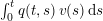 $\int _{0}^{t}q(t,s)\,v(s)\,\text{d}s$
at
 $t=t_{n}$
. Denote
 $\Vert G\Vert =\Vert G\Vert _{{\mathcal{L}}(X;Y)}$
and
 $\Vert q\Vert =\Vert q\Vert _{C(I\times I;{\mathcal{L}}(X))}$
. The trapezoidal rule for a continuous function
 $w(t)$
is
 $$\begin{eqnarray}\int _{0}^{t_{n}}w(s)\,\text{d}s\approx k\mathop{\sum }_{i=0}^{n}\hspace{-1.0pt}\text{}^{\prime }w_{i},\quad 1\leq n\leq N,\end{eqnarray}$$
where a prime indicates that in the summation, the first and the last terms are to be halved. Then
 ${\mathcal{S}}_{n}:={\mathcal{S}}(t_{n})$
is approximated by
 ${\mathcal{S}}_{n}^{k}$
defined by the relation
 $$\begin{eqnarray}{\mathcal{S}}_{n}^{k}v:=G\biggl(k\mathop{\sum }_{i=0}^{n}\hspace{-1.0pt}\text{}^{\prime }q(t_{n},t_{i})v_{i}+a_{{\mathcal{S}}}\biggr),\quad 1\leq n\leq N,\end{eqnarray}$$
for a grid function
 $v=\{v_{n}\}_{n=0}^{N}$
. Note that
 ${\mathcal{S}}_{0}^{k}v=G(a_{{\mathcal{S}}})$
. For a continuous function
 $v\in C(I;X)$
, we define
 ${\mathcal{S}}_{n}^{k}v$
by (5.14) with
 $v_{i}=v(t_{i})$
,
 $0\leq i\leq n$
.
Consider the following temporally semi-discrete scheme for Problem 5.3.
Problem 5.5. Find
 $u^{k}:=\{u_{n}^{k_{}^{}\}}\subset K$
such that
 $$\begin{eqnarray}\displaystyle & & \displaystyle \langle Au_{n}^{k},v-u_{n}^{k}\rangle +\unicode[STIX]{x1D711}({\mathcal{S}}_{n}^{k}u^{k},u_{n}^{k},v)-\unicode[STIX]{x1D711}({\mathcal{S}}_{n}^{k}u^{k},u_{n}^{k},u_{n}^{k})\nonumber\\ \displaystyle & & \displaystyle \quad +j^{0}(\unicode[STIX]{x1D6FE}_{j}u_{n}^{k};\unicode[STIX]{x1D6FE}_{j}v-\unicode[STIX]{x1D6FE}_{j}u_{n}^{k})\geq \langle f_{n},v-u_{n}^{k}\rangle \quad \text{for all}~v\in K.\end{eqnarray}$$
Regarding the solution existence and uniqueness for Problem 5.5, we have the following result.
Theorem 5.6. Keep the assumptions stated in Theorem 5.4. If the time step-size is such that
 $$\begin{eqnarray}k<\displaystyle \frac{2(m_{A}-\unicode[STIX]{x1D6FC}_{\unicode[STIX]{x1D711}}-\unicode[STIX]{x1D6FC}_{j}c_{j}^{2})}{\unicode[STIX]{x1D6FD}_{\unicode[STIX]{x1D711}}\Vert G\Vert \Vert q\Vert },\end{eqnarray}$$
then Problem 5.5 has a unique solution.
Proof. We prove the result via induction. The following arguments also apply to show the existence and uniqueness of
 $u_{0}^{k}$
. For
 $n\geq 1$
, with
 ${\{u_{i}^{k}\}}_{i\leq n-1}$
known, let us show that the inequality (5.15) uniquely determines
 $u_{n}^{k}\in K$
. The proof is completed via an application of the Banach fixed-point theorem.
For any
 $\unicode[STIX]{x1D702}\in X$
, denote
 $$\begin{eqnarray}y_{\unicode[STIX]{x1D702}}={\mathcal{S}}_{n}^{k}u^{k\unicode[STIX]{x1D702}},\end{eqnarray}$$
where
 $u^{k\unicode[STIX]{x1D702}}=\{u_{0}^{k},\ldots ,u_{n-1}^{k},\unicode[STIX]{x1D702}\}$
. According to Theorem 4.4, we know that there exists a unique
 $u_{\unicode[STIX]{x1D702}}\in K$
such that
 $$\begin{eqnarray}\displaystyle & & \displaystyle \langle Au_{\unicode[STIX]{x1D702}},v-u_{\unicode[STIX]{x1D702}}\rangle +\unicode[STIX]{x1D711}(y_{\unicode[STIX]{x1D702}},u_{\unicode[STIX]{x1D702}},v)-\unicode[STIX]{x1D711}(y_{\unicode[STIX]{x1D702}},u_{\unicode[STIX]{x1D702}},u_{\unicode[STIX]{x1D702}})\nonumber\\ \displaystyle & & \displaystyle \quad +j^{0}(\unicode[STIX]{x1D6FE}_{j}u_{\unicode[STIX]{x1D702}};\unicode[STIX]{x1D6FE}_{j}v-\unicode[STIX]{x1D6FE}_{j}u_{\unicode[STIX]{x1D702}})\geq \langle f_{n},v-u_{\unicode[STIX]{x1D702}}\rangle \quad \text{for all}~v\in K\end{eqnarray}$$
under the stated assumptions, where
 $f_{n}=f(t_{n})$
. This allows us to define an operator
 $\unicode[STIX]{x1D6EC}:X\rightarrow K$
by
 $$\begin{eqnarray}\unicode[STIX]{x1D6EC}\unicode[STIX]{x1D702}=u_{\unicode[STIX]{x1D702}}.\end{eqnarray}$$
Let us show that
 $\unicode[STIX]{x1D6EC}$
is a contractive mapping. For any
 $\unicode[STIX]{x1D702}_{1},\unicode[STIX]{x1D702}_{2}\in X$
, denote
 $y_{i}=y_{\unicode[STIX]{x1D702}_{i}}$
,
 $u_{i}=u_{\unicode[STIX]{x1D702}_{i}}$
,
 $u^{k\unicode[STIX]{x1D702}_{i}}=\{u_{0}^{k},\ldots ,u_{n-1}^{k},\unicode[STIX]{x1D702}_{i}\}$
,
 $i=1,2$
. Then
 $u_{1}\in K$
satisfies
 $$\begin{eqnarray}\displaystyle & & \displaystyle \langle Au_{1},v-u_{1}\rangle +\unicode[STIX]{x1D711}(y_{1},u_{1},v)-\unicode[STIX]{x1D711}(y_{1},u_{1},u_{1})\nonumber\\ \displaystyle & & \displaystyle \quad +j^{0}(\unicode[STIX]{x1D6FE}_{j}u_{1};\unicode[STIX]{x1D6FE}_{j}v-\unicode[STIX]{x1D6FE}_{j}u_{1})\geq \langle f_{n},v-u_{1}\rangle \quad \text{for all}~v\in K,\end{eqnarray}$$
and
 $u_{2}\in K$
satisfies
 $$\begin{eqnarray}\displaystyle & & \displaystyle \langle Au_{2},v-u_{2}\rangle +\unicode[STIX]{x1D711}(y_{2},u_{2},v)-\unicode[STIX]{x1D711}(y_{2},u_{2},u_{2})\nonumber\\ \displaystyle & & \displaystyle \quad +j^{0}(\unicode[STIX]{x1D6FE}_{j}u_{2};\unicode[STIX]{x1D6FE}_{j}v-\unicode[STIX]{x1D6FE}_{j}u_{2})\geq \langle f_{n},v-u_{2}\rangle \quad \text{for all}~v\in K.\end{eqnarray}$$
Take
 $v=u_{2}$
in (5.20) and
 $v=u_{1}$
in (5.21), and add the two inequalities to obtain
 $$\begin{eqnarray}\displaystyle \langle Au_{1}-Au_{2},u_{1}-u_{2}\rangle & \leq & \displaystyle \unicode[STIX]{x1D711}(y_{1},u_{1},u_{2})-\unicode[STIX]{x1D711}(y_{1},u_{1},u_{1})\nonumber\\ \displaystyle & & \displaystyle +\,\unicode[STIX]{x1D711}(y_{2},u_{2},u_{1})-\unicode[STIX]{x1D711}(y_{2},u_{2},u_{2})\nonumber\\ \displaystyle & & \displaystyle +\,j^{0}(\unicode[STIX]{x1D6FE}_{j}u_{1};\unicode[STIX]{x1D6FE}_{j}u_{2}-\unicode[STIX]{x1D6FE}_{j}u_{1})+j^{0}(\unicode[STIX]{x1D6FE}_{j}u_{2};\unicode[STIX]{x1D6FE}_{j}u_{1}-\unicode[STIX]{x1D6FE}_{j}u_{2}).\nonumber\end{eqnarray}$$
We use assumptions (4.2(b)), (5.3(b)) and (4.19(c)) to get
 $$\begin{eqnarray}(m_{A}-\unicode[STIX]{x1D6FC}_{\unicode[STIX]{x1D711}}-\unicode[STIX]{x1D6FC}_{j}c_{j}^{2})\Vert u_{1}-u_{2}\Vert _{X}\leq \unicode[STIX]{x1D6FD}_{\unicode[STIX]{x1D711}}\Vert y_{1}-y_{2}\Vert _{Y}.\end{eqnarray}$$
This inequality can be rewritten as
 $$\begin{eqnarray}\Vert \unicode[STIX]{x1D6EC}\unicode[STIX]{x1D702}_{1}-\unicode[STIX]{x1D6EC}\unicode[STIX]{x1D702}_{2}\Vert _{X}\leq \displaystyle \frac{\unicode[STIX]{x1D6FD}_{\unicode[STIX]{x1D711}}}{m_{A}-\unicode[STIX]{x1D6FC}_{\unicode[STIX]{x1D711}}-\unicode[STIX]{x1D6FC}_{j}c_{j}^{2}}\Vert y_{1}-y_{2}\Vert _{Y}.\end{eqnarray}$$
Now,
 $$\begin{eqnarray}\displaystyle y_{1}-y_{2} & = & \displaystyle {\mathcal{S}}_{n}^{k}u^{k\unicode[STIX]{x1D702}_{1}}-{\mathcal{S}}_{n}^{k}u^{k\unicode[STIX]{x1D702}_{2}}\nonumber\\ \displaystyle & = & \displaystyle G\biggl(k\mathop{\sum }_{i=0}^{n}\hspace{-1.0pt}\text{}^{\prime }q(t_{n},t_{i})u_{i}^{k\unicode[STIX]{x1D702}_{1}}+a_{{\mathcal{S}}}\biggr)-G\biggl(k\mathop{\sum }_{i=0}^{n}\hspace{-1.0pt}\text{}^{\prime }q(t_{n},t_{i})u_{i}^{k\unicode[STIX]{x1D702}_{2}}+a_{{\mathcal{S}}}\biggr).\nonumber\end{eqnarray}$$
Then,
 $$\begin{eqnarray}\Vert y_{1}-y_{2}\Vert _{Y}\leq \displaystyle \frac{k}{2}\,\Vert G\Vert \,\Vert q\Vert \,\Vert \unicode[STIX]{x1D702}_{1}-\unicode[STIX]{x1D702}_{2}\Vert _{X}.\end{eqnarray}$$
Use (5.23) in (5.22) to obtain
 $$\begin{eqnarray}\Vert \unicode[STIX]{x1D6EC}\unicode[STIX]{x1D702}_{1}-\unicode[STIX]{x1D6EC}\unicode[STIX]{x1D702}_{2}\Vert _{X}\leq \displaystyle \frac{k}{2}\,\displaystyle \frac{\unicode[STIX]{x1D6FD}_{\unicode[STIX]{x1D711}}}{m_{A}-\unicode[STIX]{x1D6FC}_{\unicode[STIX]{x1D711}}-\unicode[STIX]{x1D6FC}_{j}c_{j}^{2}}\,\Vert G\Vert \Vert q\Vert \Vert \unicode[STIX]{x1D702}_{1}-\unicode[STIX]{x1D702}_{2}\Vert _{X}.\end{eqnarray}$$
By the smallness condition (5.16),
 $$\begin{eqnarray}\displaystyle \frac{k}{2}\,\displaystyle \frac{\unicode[STIX]{x1D6FD}_{\unicode[STIX]{x1D711}}}{m_{A}-\unicode[STIX]{x1D6FC}_{\unicode[STIX]{x1D711}}-\unicode[STIX]{x1D6FC}_{j}c_{j}^{2}}\,\Vert G\Vert \Vert q\Vert <1.\end{eqnarray}$$
Applying Theorem 3.19, we conclude that the operator
 $\unicode[STIX]{x1D6EC}$
has a unique fixed point
 $\unicode[STIX]{x1D702}^{\ast }\in K$
. By the definitions (5.17) and (5.19),
 $$\begin{eqnarray}y_{\unicode[STIX]{x1D702}^{\ast }}={\mathcal{S}}_{n}^{k}u^{k\unicode[STIX]{x1D702}^{\ast }},\quad u_{\unicode[STIX]{x1D702}^{\ast }}=\unicode[STIX]{x1D702}^{\ast }.\end{eqnarray}$$
Considering the inequality (5.18) with
 $\unicode[STIX]{x1D702}=\unicode[STIX]{x1D702}^{\ast }$
, we know that
 $u_{n}^{k}=\unicode[STIX]{x1D702}^{\ast }\in K$
is the unique solution of (5.15).◻
Before deriving an error bound for the semi-discrete solution defined by Problem 5.5, we present a preliminary result.
Lemma 5.7. Let
 ${\mathcal{S}}:C(I;X)\rightarrow C(I;Y)$
be defined by (5.12) and let
 ${\mathcal{S}}_{n}^{k}$
be defined by (5.14), where
 $G\in {\mathcal{L}}(X;Y)$
,
 $q\in C^{2}(I\times I;{\mathcal{L}}(X))$
,
 $a_{{\mathcal{S}}}\in X$
. Assume
 $u\in W^{2,\infty }(I;X)$
. Then for a constant
 $c$
depending on
 $G$
and
 $q$
,
 $$\begin{eqnarray}\Vert {\mathcal{S}}_{n}u-{\mathcal{S}}_{n}^{k}u\Vert _{Y}\leq c\,k^{2}\Vert u\Vert _{W^{2,\infty }(I;X)}.\end{eqnarray}$$
Proof. By definition,
 $$\begin{eqnarray}{\mathcal{S}}_{n}u-{\mathcal{S}}_{n}^{k}u=G\biggl(\int _{0}^{t}q(t,s)\,u(s)\,\text{d}s+a_{{\mathcal{S}}}\biggr)-G\biggl(k\mathop{\sum }_{i=0}^{n}\hspace{-1.0pt}\text{}^{\prime }q(t_{n},t_{i})u_{i}+a_{{\mathcal{S}}}\biggr).\end{eqnarray}$$
Then,
 $$\begin{eqnarray}\Vert {\mathcal{S}}_{n}u-{\mathcal{S}}_{n}^{k}u\Vert _{Y}\leq \Vert G\Vert \,\mathop{\biggl\|\int _{0}^{t_{n}}q(t_{n},s)\,u(s)\,\text{d}s-k\mathop{\sum }_{i=0}^{n}\hspace{-1.0pt}\text{}^{\prime }q(t_{n},t_{i})\,u_{i}\biggr\|}\nolimits_{X}.\end{eqnarray}$$
With the use of Taylor’s expansion on each of the subintervals
 $[0,t_{1}]$
,
 $[t_{1},t_{2}]$
,
 $\ldots ,$
 $[t_{n-1},t_{n}]$
, we find that
 $$\begin{eqnarray}\displaystyle & & \displaystyle \mathop{\biggl\|\int _{0}^{t_{n}}q(t_{n},s)\,u(s)\,\text{d}s-k\mathop{\sum }_{i=0}^{n}\hspace{-1.0pt}\text{}^{\prime }q(t_{n},t_{i})\,u_{i}\biggr\|}\nolimits_{X}\nonumber\\ \displaystyle & & \displaystyle \quad \leq c\,k^{2}\biggl\|\biggl(\displaystyle \frac{\text{d}}{\text{d}s}\biggr)^{2}[q(t_{n},s)\,u(s)]\biggr\|_{L^{\infty }((0,t_{n});X)}.\nonumber\end{eqnarray}$$
Thus, (5.26) holds.◻
Theorem 5.8. Keep the assumptions of Theorem 5.4 and Lemma 5.7. Then for the semi-discrete solution of Problem 5.5, we have the following error bound:
 $$\begin{eqnarray}\max _{0\leq n\leq N}\Vert u_{n}-u_{n}^{k}\Vert _{X}\leq c\,k^{2}.\end{eqnarray}$$
Proof. We take
 $v=u_{n}^{k}$
in the inequality (5.10) at
 $t=t_{n}$
to get
 $$\begin{eqnarray}\displaystyle & & \displaystyle \langle Au_{n},u_{n}^{k}-u_{n}\rangle +\unicode[STIX]{x1D711}({\mathcal{S}}_{n}u,u_{n},u_{n}^{k})-\unicode[STIX]{x1D711}({\mathcal{S}}_{n}u,u_{n},u_{n})\nonumber\\ \displaystyle & & \displaystyle \quad +j^{0}(\unicode[STIX]{x1D6FE}_{j}u_{n};\unicode[STIX]{x1D6FE}_{j}u_{n}^{k}-\unicode[STIX]{x1D6FE}_{j}u_{n})\geq \langle f_{n},u_{n}^{k}-u_{n}\rangle ,\end{eqnarray}$$
where
 ${\mathcal{S}}_{n}u=G(\int _{0}^{t_{n}}q(t_{n},s)\,u(s)\,\text{d}s+a_{S})$
. Take
 $v=u_{n}$
in (5.15),
 $$\begin{eqnarray}\displaystyle & & \displaystyle \langle Au_{n}^{k},u_{n}-u_{n}^{k}\rangle +\unicode[STIX]{x1D711}({\mathcal{S}}_{n}^{k}u^{k},u_{n}^{k},u_{n})-\unicode[STIX]{x1D711}({\mathcal{S}}_{n}^{k}u^{k},u_{n}^{k},u_{n}^{k})\nonumber\\ \displaystyle & & \displaystyle \quad +j^{0}(\unicode[STIX]{x1D6FE}_{j}u_{n}^{k};\unicode[STIX]{x1D6FE}_{j}u_{n}-\unicode[STIX]{x1D6FE}_{j}u_{n}^{k})\geq \langle f_{n},u_{n}-u_{n}^{k}\rangle .\end{eqnarray}$$
 $$\begin{eqnarray}\displaystyle \langle Au_{n}-Au_{n}^{k},u_{n}-u_{n}^{k}\rangle & \leq & \displaystyle \unicode[STIX]{x1D711}({\mathcal{S}}_{n}u,u_{n},u_{n}^{k})-\unicode[STIX]{x1D711}({\mathcal{S}}_{n}u,u_{n},u_{n})\nonumber\\ \displaystyle & & \displaystyle \quad ~~+\unicode[STIX]{x1D711}({\mathcal{S}}_{n}^{k}u^{k},u_{n}^{k},u_{n})-\unicode[STIX]{x1D711}({\mathcal{S}}_{n}^{k}u^{k},u_{n}^{k},u_{n}^{k})\nonumber\\ \displaystyle & & \displaystyle \quad ~~+j^{0}(\unicode[STIX]{x1D6FE}_{j}u_{n};\unicode[STIX]{x1D6FE}_{j}u_{n}^{k}-\unicode[STIX]{x1D6FE}_{j}u_{n})+j^{0}(\unicode[STIX]{x1D6FE}_{j}u_{n}^{k};\unicode[STIX]{x1D6FE}_{j}u_{n}-\unicode[STIX]{x1D6FE}_{j}u_{n}^{k}).\nonumber\end{eqnarray}$$
By (4.2(b)),
 $$\begin{eqnarray}m_{A}\Vert u_{n}-u_{n}^{k}\Vert _{X}^{2}\leq \langle Au_{n}-Au_{n}^{k},u_{n}-u_{n}^{k}\rangle .\end{eqnarray}$$
By (5.3(b)),
 $$\begin{eqnarray}\displaystyle & & \displaystyle \unicode[STIX]{x1D711}({\mathcal{S}}_{n}u,u_{n},u_{n}^{k})-\unicode[STIX]{x1D711}({\mathcal{S}}_{n}u,u_{n},u_{n})+\unicode[STIX]{x1D711}({\mathcal{S}}_{n}^{k}u^{k},u_{n}^{k},u_{n})-\unicode[STIX]{x1D711}({\mathcal{S}}_{n}^{k}u^{k},u_{n}^{k},u_{n}^{k})\nonumber\\ \displaystyle & & \displaystyle \quad \leq \unicode[STIX]{x1D6FC}_{\unicode[STIX]{x1D711}}\Vert u_{n}-u_{n}^{k}\Vert _{X}^{2}+\unicode[STIX]{x1D6FD}_{\unicode[STIX]{x1D711}}\Vert {\mathcal{S}}_{n}u-{\mathcal{S}}_{n}^{k}u^{k}\Vert _{Y}\Vert u_{n}-u_{n}^{k}\Vert _{X}.\nonumber\end{eqnarray}$$
 $$\begin{eqnarray}j^{0}(\unicode[STIX]{x1D6FE}_{j}u_{n};\unicode[STIX]{x1D6FE}_{j}u_{n}^{k}-\unicode[STIX]{x1D6FE}_{j}u_{n})+j^{0}(\unicode[STIX]{x1D6FE}_{j}u_{n}^{k};\unicode[STIX]{x1D6FE}_{j}u_{n}-\unicode[STIX]{x1D6FE}_{j}u_{n}^{k})\leq \unicode[STIX]{x1D6FC}_{j}c_{j}^{2}\Vert u_{n}-u_{n}^{k}\Vert _{X}^{2}.\end{eqnarray}$$
Thus,
 $$\begin{eqnarray}\displaystyle m_{A}\Vert u_{n}-u_{n}^{k}\Vert _{X}^{2} & \leq & \displaystyle \unicode[STIX]{x1D6FC}_{\unicode[STIX]{x1D711}}\Vert u_{n}-u_{n}^{k}\Vert _{X}^{2}+\unicode[STIX]{x1D6FD}_{\unicode[STIX]{x1D711}}\Vert {\mathcal{S}}_{n}u-{\mathcal{S}}_{n}^{k}u^{k}\Vert _{Y}\Vert u_{n}-u_{n}^{k}\Vert _{X}\nonumber\\ \displaystyle & & \displaystyle +\,\unicode[STIX]{x1D6FC}_{j}c_{j}^{2}\Vert u_{n}-u_{n}^{k}\Vert _{X}^{2}\nonumber\end{eqnarray}$$
or, equivalently,
 $$\begin{eqnarray}(m_{A}-\unicode[STIX]{x1D6FC}_{\unicode[STIX]{x1D711}}-\unicode[STIX]{x1D6FC}_{j}c_{j}^{2})\Vert u_{n}-u_{n}^{k}\Vert _{X}\leq \unicode[STIX]{x1D6FD}_{\unicode[STIX]{x1D711}}\Vert {\mathcal{S}}_{n}u-{\mathcal{S}}_{n}^{k}u^{k}\Vert _{Y}.\end{eqnarray}$$
Write
 $$\begin{eqnarray}\Vert {\mathcal{S}}_{n}u-{\mathcal{S}}_{n}^{k}u^{k}\Vert _{Y}\leq \Vert {\mathcal{S}}_{n}u-{\mathcal{S}}_{n}^{k}u\Vert _{Y}+\Vert {\mathcal{S}}_{n}^{k}u-{\mathcal{S}}_{n}^{k}u^{k}\Vert _{Y}.\end{eqnarray}$$
By Lemma 5.7,
 $$\begin{eqnarray}\Vert {\mathcal{S}}_{n}u-{\mathcal{S}}_{n}^{k}u\Vert _{Y}\leq c\,k^{2}\Vert u\Vert _{W^{2,\infty }(I;X)}.\end{eqnarray}$$
It is easy to see that
 $$\begin{eqnarray}\Vert {\mathcal{S}}_{n}^{k}u-{\mathcal{S}}_{n}^{k}u^{k}\Vert _{Y}\leq k\,\Vert G\Vert \,\Vert q\Vert \mathop{\sum }_{i=0}^{n}\Vert u_{i}-u_{i}^{k}\Vert _{X}.\end{eqnarray}$$
Hence,
 $$\begin{eqnarray}\Vert {\mathcal{S}}_{n}u-{\mathcal{S}}_{n}^{k}u^{k}\Vert _{Y}\leq c\,k^{2}\Vert u\Vert _{W^{2,\infty }(I;X)}+k\Vert G\Vert \Vert q\Vert \mathop{\sum }_{i=0}^{n}\Vert u_{i}-u_{i}^{k}\Vert _{X}.\end{eqnarray}$$
Using (5.31) in (5.30), we get
 $$\begin{eqnarray}\Vert u_{n}-u_{n}^{k}\Vert _{X}\leq k^{2}\displaystyle \frac{c\,\unicode[STIX]{x1D6FD}_{\unicode[STIX]{x1D711}}\Vert u\Vert _{W^{2,\infty }(I;X)}}{m_{A}-\unicode[STIX]{x1D6FC}_{\unicode[STIX]{x1D711}}-\unicode[STIX]{x1D6FC}_{j}c_{j}^{2}}+k\displaystyle \frac{\unicode[STIX]{x1D6FD}_{\unicode[STIX]{x1D711}}\Vert G\Vert \Vert q\Vert }{m_{A}-\unicode[STIX]{x1D6FC}_{\unicode[STIX]{x1D711}}-\unicode[STIX]{x1D6FC}_{j}c_{j}^{2}}\mathop{\sum }_{i=0}^{n}\Vert u_{i}-u_{i}^{k}\Vert _{X}.\end{eqnarray}$$
We then apply the discrete Gronwall’s inequality (see Lemma 3.24) to derive the error bound (5.27) from (5.32).◻
5.3 Fully discrete approximation
Now we consider fully discrete approximations of Problem 5.3. In a fully discrete scheme, both the temporal and spatial variables are discretized. In addition to the notation and assumptions stated in Section 5.2 for the temporal discretization, we introduce a regular family of finite element partitions
 $\{{\mathcal{T}}^{h}\}$
for the spatial discretization. We use a finite element space
 $X^{h}\subset X$
that corresponds to the partition
 ${\mathcal{T}}^{h}$
and use a non-empty, convex and closed subset
 $K^{h}\subset X^{h}$
to approximate
 $K$
. Focusing on internal approximations, we assume
 $K^{h}\subset K$
. External approximations can be also considered, as in Section 4.
Apply the operator
 ${\mathcal{S}}_{n}^{k}$
defined in (5.14) on
 $u^{hk}=\{u_{n}^{hk_{}^{}\}}\subset X^{h}$
:
 $$\begin{eqnarray}{\mathcal{S}}_{n}^{k}u^{hk}:=G\biggl(k\mathop{\sum }_{i=0}^{n}\hspace{-1.0pt}\text{}^{\prime }q(t_{n},t_{i})u_{i}^{hk}+a_{{\mathcal{S}}}\biggr).\end{eqnarray}$$
We then introduce a fully discrete approximation of Problem 5.3 as follows.
Problem 5.9. Find
 $u^{hk}:=\{u_{n}^{hk_{}^{}\}}\subset K^{h}$
such that
 $$\begin{eqnarray}\displaystyle & & \displaystyle \langle Au_{n}^{hk},v^{h}-u_{n}^{hk}\rangle +\unicode[STIX]{x1D711}({\mathcal{S}}_{n}^{k}u^{hk},u_{n}^{hk},v^{h})-\unicode[STIX]{x1D711}({\mathcal{S}}_{n}^{k}u^{hk},u_{n}^{hk},u_{n}^{hk})\nonumber\\ \displaystyle & & \displaystyle \quad +j^{0}(\unicode[STIX]{x1D6FE}_{j}u_{n}^{hk};\unicode[STIX]{x1D6FE}_{j}v^{h}-\unicode[STIX]{x1D6FE}_{j}u_{n}^{hk})\geq \langle f_{n},v^{h}-u_{n}^{hk}\rangle \quad \text{for all}~v^{h}\in K^{h}.\end{eqnarray}$$
As in Theorem 5.6, Problem 5.9 has a unique solution under the assumptions stated in Theorem 5.6. Next we derive an error bound for the fully discrete scheme.
Theorem 5.10. Keep the assumptions stated in Theorem 5.4. Moreover, assume
 $A:X\rightarrow X^{\ast }$
is Lipschitz continuous,
 $q\in C^{2}(I\times I;{\mathcal{L}}(X))$
, and
 $u\in W^{2,\infty }(I;X)$
. Then for
 $k$
sufficiently small, we have the error bound
 $$\begin{eqnarray}\displaystyle & & \displaystyle \max _{0\leq n\leq N}\Vert u_{n}-u_{n}^{hk}\Vert _{X}\nonumber\\ \displaystyle & & \displaystyle \leq c\max _{0\leq n\leq N}\inf _{v^{h}\in K^{h}}\big[\Vert u_{n}-v^{h}\Vert _{X}+\Vert \unicode[STIX]{x1D6FE}_{j}(u_{n}-v^{h})\Vert _{X_{j}}^{1/2}+|R_{n}(v^{h},u_{n})|^{1/2}\big]+c\,k^{2},\end{eqnarray}$$
where the residual-type term
 $R_{n}(v^{h},u_{n})$
is defined by
 $$\begin{eqnarray}\displaystyle R_{n}(v^{h},u_{n}) & = & \displaystyle \langle Au_{n},v^{h}-u_{n}\rangle +\unicode[STIX]{x1D711}({\mathcal{S}}_{n}u,u_{n},v^{h})-\unicode[STIX]{x1D711}({\mathcal{S}}_{n}u,u_{n},u_{n})\nonumber\\ \displaystyle & & \displaystyle +\,j^{0}(\unicode[STIX]{x1D6FE}_{j}u_{n};\unicode[STIX]{x1D6FE}_{j}v^{h}-\unicode[STIX]{x1D6FE}_{j}u_{n})-\langle f_{n},v^{h}-u_{n}\rangle .\end{eqnarray}$$
Proof. By (4.2(b)),
 $$\begin{eqnarray}m_{A}\Vert u_{n}-u_{n}^{hk}\Vert _{X}^{2}\leq \langle Au_{n}-Au_{n}^{hk},u_{n}-u_{n}^{hk}\rangle .\end{eqnarray}$$
Write
 $$\begin{eqnarray}\displaystyle \langle Au_{n}-Au_{n}^{hk},u_{n}-u_{n}^{hk}\rangle & = & \displaystyle \langle Au_{n}-Au_{n}^{hk},u_{n}-v^{h}\rangle +\langle Au_{n},v^{h}-u_{n}\rangle \nonumber\\ \displaystyle & & \displaystyle +\,\langle Au_{n},u_{n}-u_{n}^{hk}\rangle +\langle Au_{n}^{hk},u_{n}^{hk}-v^{h}\rangle .\end{eqnarray}$$
Take
 $v=u_{n}^{hk}$
in (5.10) at
 $t=t_{n}$
,
 $$\begin{eqnarray}\displaystyle & & \displaystyle \langle Au_{n},u_{n}^{hk}-u_{n}\rangle +\unicode[STIX]{x1D711}({\mathcal{S}}_{n}u,u_{n},u_{n}^{hk})-\unicode[STIX]{x1D711}({\mathcal{S}}_{n}u,u_{n},u_{n})\nonumber\\ \displaystyle & & \displaystyle +\,j^{0}(\unicode[STIX]{x1D6FE}_{j}u_{n};\unicode[STIX]{x1D6FE}_{j}u_{n}^{hk}-\unicode[STIX]{x1D6FE}_{j}u_{n})\geq \langle f_{n},u_{n}^{hk}-u_{n}\rangle ,\nonumber\end{eqnarray}$$
that is,
 $$\begin{eqnarray}\displaystyle \langle Au_{n},u_{n}-u_{n}^{hk}\rangle & \leq & \displaystyle \unicode[STIX]{x1D711}({\mathcal{S}}_{n}u,u_{n},u_{n}^{hk})-\unicode[STIX]{x1D711}({\mathcal{S}}_{n}u,u_{n},u_{n})\nonumber\\ \displaystyle & & \displaystyle +\,j^{0}(\unicode[STIX]{x1D6FE}_{j}u_{n};\unicode[STIX]{x1D6FE}_{j}u_{n}^{hk}-\unicode[STIX]{x1D6FE}_{j}u_{n})-\langle f_{n},u_{n}-u_{n}^{hk}\rangle .\end{eqnarray}$$
From (5.34),
 $$\begin{eqnarray}\displaystyle \langle Au_{n}^{hk},u_{n}^{hk}-v^{h}\rangle & \leq & \displaystyle \unicode[STIX]{x1D711}({\mathcal{S}}_{n}^{k}u^{hk},u_{n}^{hk},v^{h})-\unicode[STIX]{x1D711}({\mathcal{S}}_{n}^{k}u^{hk},u_{n}^{hk},u_{n}^{hk})\nonumber\\ \displaystyle & & \displaystyle +\,j^{0}(\unicode[STIX]{x1D6FE}_{j}u_{n}^{hk};\unicode[STIX]{x1D6FE}_{j}v^{h}-\unicode[STIX]{x1D6FE}_{j}u_{n}^{hk})-\langle f_{n},v^{h}-u_{n}^{hk}\rangle .\end{eqnarray}$$
Combining (5.37), (5.38), (5.39) and (5.40), we get
 $$\begin{eqnarray}\displaystyle m_{A}\Vert u_{n}-u_{n}^{hk}\Vert _{X}^{2} & \leq & \displaystyle \langle Au_{n}-Au_{n}^{hk},u_{n}-v^{h}\rangle +R_{n}(v^{h},u_{n})\nonumber\\ \displaystyle & & \displaystyle +\,E_{\unicode[STIX]{x1D711}_{1}}+E_{\unicode[STIX]{x1D711}_{2}}+E_{j},\end{eqnarray}$$
where
 $R_{n}(v^{h},u_{n})$
is defined in (5.36), and
 $$\begin{eqnarray}\displaystyle E_{\unicode[STIX]{x1D711}_{1}} & = & \displaystyle \unicode[STIX]{x1D711}({\mathcal{S}}_{n}u,u_{n},u_{n}^{hk})-\unicode[STIX]{x1D711}({\mathcal{S}}_{n}u,u_{n},u_{n})\nonumber\\ \displaystyle & & \displaystyle +\,\unicode[STIX]{x1D711}({\mathcal{S}}_{n}^{k}u^{hk},u_{n}^{hk},u_{n})-\unicode[STIX]{x1D711}({\mathcal{S}}_{n}^{k}u^{hk},u_{n}^{hk},u_{n}^{hk}),\end{eqnarray}$$
 $$\begin{eqnarray}\displaystyle E_{\unicode[STIX]{x1D711}_{2}} & = & \displaystyle \unicode[STIX]{x1D711}({\mathcal{S}}_{n}^{k}u^{hk},u_{n}^{hk},v^{h})-\unicode[STIX]{x1D711}({\mathcal{S}}_{n}^{k}u^{hk},u_{n}^{hk},u_{n})\nonumber\\ \displaystyle & & \displaystyle +\,\unicode[STIX]{x1D711}({\mathcal{S}}_{n}u,u_{n},u_{n})-\unicode[STIX]{x1D711}({\mathcal{S}}_{n}u,u_{n},v^{h}),\end{eqnarray}$$
 $$\begin{eqnarray}\displaystyle E_{j} & = & \displaystyle j^{0}(\unicode[STIX]{x1D6FE}_{j}u_{n};\unicode[STIX]{x1D6FE}_{j}u_{n}^{hk}-\unicode[STIX]{x1D6FE}_{j}u_{n})+j^{0}(\unicode[STIX]{x1D6FE}_{j}u_{n}^{hk};\unicode[STIX]{x1D6FE}_{j}v^{h}-\unicode[STIX]{x1D6FE}_{j}u_{n}^{hk})\nonumber\\ \displaystyle & & \displaystyle -\,j^{0}(\unicode[STIX]{x1D6FE}_{j}u_{n};\unicode[STIX]{x1D6FE}_{j}v^{h}-\unicode[STIX]{x1D6FE}_{j}u_{n}).\end{eqnarray}$$
Let us bound each of the terms on the right-hand side of (5.41). Let
 $L_{A}>0$
denote the Lipschitz constant of the operator
 $A$
. Then
 $$\begin{eqnarray}\langle Au_{n}-Au_{n}^{hk},u_{n}-v^{h}\rangle \leq L_{A}\Vert u_{n}-u_{n}^{hk}\Vert _{X}\Vert u_{n}-v^{h}\Vert _{X}.\end{eqnarray}$$
By (5.3(b)),
 $$\begin{eqnarray}\displaystyle E_{\unicode[STIX]{x1D711}_{1}} & \leq & \displaystyle \unicode[STIX]{x1D6FC}_{\unicode[STIX]{x1D711}}\Vert u_{n}-u_{n}^{hk}\Vert _{X}^{2}+\unicode[STIX]{x1D6FD}_{\unicode[STIX]{x1D711}}\Vert {\mathcal{S}}_{n}u-{\mathcal{S}}_{n}^{k}u^{hk}\Vert _{Y}\Vert u_{n}-u_{n}^{hk}\Vert _{X},\end{eqnarray}$$
 $$\begin{eqnarray}\displaystyle E_{\unicode[STIX]{x1D711}_{2}} & \leq & \displaystyle (\unicode[STIX]{x1D6FC}_{\unicode[STIX]{x1D711}}\Vert u_{n}-u_{n}^{hk}\Vert _{X}+\unicode[STIX]{x1D6FD}_{\unicode[STIX]{x1D711}}\Vert {\mathcal{S}}_{n}u-{\mathcal{S}}_{n}^{k}u^{hk}\Vert _{Y})\Vert u_{n}-v^{h}\Vert _{X}.\end{eqnarray}$$
By the subadditivity of the generalized directional derivative (see Proposition 3.10),
 $$\begin{eqnarray}\displaystyle j^{0}(\unicode[STIX]{x1D6FE}_{j}u_{n}^{hk};\unicode[STIX]{x1D6FE}_{j}v^{h}-\unicode[STIX]{x1D6FE}_{j}u_{n}^{hk}) & \leq & \displaystyle j^{0}(\unicode[STIX]{x1D6FE}_{j}u_{n}^{hk};\unicode[STIX]{x1D6FE}_{j}u_{n}-\unicode[STIX]{x1D6FE}_{j}u_{n}^{hk})\nonumber\\ \displaystyle & & \displaystyle +\,j^{0}(\unicode[STIX]{x1D6FE}_{j}u_{n}^{hk};\unicode[STIX]{x1D6FE}_{j}v^{h}-\unicode[STIX]{x1D6FE}_{j}u_{n}).\nonumber\end{eqnarray}$$
Thus,
 $$\begin{eqnarray}\displaystyle E_{j} & \leq & \displaystyle j^{0}(\unicode[STIX]{x1D6FE}_{j}u_{n};\unicode[STIX]{x1D6FE}_{j}u_{n}^{hk}-\unicode[STIX]{x1D6FE}_{j}u_{n})+j^{0}(\unicode[STIX]{x1D6FE}_{j}u_{n}^{hk};\unicode[STIX]{x1D6FE}_{j}u_{n}-\unicode[STIX]{x1D6FE}_{j}u_{n}^{hk})\nonumber\\ \displaystyle & & \displaystyle +\,j^{0}(\unicode[STIX]{x1D6FE}_{j}u_{n}^{hk};\unicode[STIX]{x1D6FE}_{j}v^{h}-\unicode[STIX]{x1D6FE}_{j}u_{n})-j^{0}(\unicode[STIX]{x1D6FE}_{j}u_{n};\unicode[STIX]{x1D6FE}_{j}v^{h}-\unicode[STIX]{x1D6FE}_{j}u_{n}).\nonumber\end{eqnarray}$$
 $$\begin{eqnarray}j^{0}(\unicode[STIX]{x1D6FE}_{j}u_{n};\unicode[STIX]{x1D6FE}_{j}u_{n}^{hk}-\unicode[STIX]{x1D6FE}_{j}u_{n})+j^{0}(\unicode[STIX]{x1D6FE}_{j}u_{n}^{hk};\unicode[STIX]{x1D6FE}_{j}u_{n}-\unicode[STIX]{x1D6FE}_{j}u_{n}^{hk})\leq \unicode[STIX]{x1D6FC}_{j}c_{j}^{2}\Vert u_{n}-u_{n}^{hk}\Vert _{X}^{2}.\end{eqnarray}$$
By (4.19(b)) and (4.17), we have
 $$\begin{eqnarray}|j^{0}(\unicode[STIX]{x1D6FE}_{j}u_{n};\unicode[STIX]{x1D6FE}_{j}v^{h}-\unicode[STIX]{x1D6FE}_{j}u_{n})|\leq (c_{0}+c_{1}c_{j}\Vert u_{n}\Vert _{X})\Vert \unicode[STIX]{x1D6FE}_{j}(u_{n}-v^{h})\Vert _{X_{j}}\end{eqnarray}$$
and
 $$\begin{eqnarray}\displaystyle |j^{0}(\unicode[STIX]{x1D6FE}_{j}u_{n}^{hk};\unicode[STIX]{x1D6FE}_{j}v^{h}-\unicode[STIX]{x1D6FE}_{j}u_{n})| & \leq & \displaystyle (c_{0}+c_{1}c_{j}\Vert u_{n}^{hk}\Vert _{X})\Vert \unicode[STIX]{x1D6FE}_{j}(u_{n}-v^{h})\Vert _{X_{j}}\nonumber\\ \displaystyle & \leq & \displaystyle c_{1}c_{j}\Vert u_{n}-u_{n}^{hk}\Vert _{X}\Vert \unicode[STIX]{x1D6FE}_{j}(u_{n}-v^{h})\Vert _{X_{j}}\nonumber\\ \displaystyle & & \displaystyle +\,(c_{0}+c_{1}c_{j}\Vert u_{n}\Vert _{X})\Vert \unicode[STIX]{x1D6FE}_{j}(u_{n}-v^{h})\Vert _{X_{j}}.\nonumber\end{eqnarray}$$
Hence,
 $$\begin{eqnarray}\displaystyle E_{j} & \leq & \displaystyle (2c_{0}+2c_{1}c_{j}\Vert u_{n}\Vert _{X})\Vert \unicode[STIX]{x1D6FE}_{j}(u_{n}-v^{h})\Vert _{X_{j}}+\unicode[STIX]{x1D6FC}_{j}c_{j}^{2}\Vert u_{n}-u_{n}^{hk}\Vert _{X}^{2}\nonumber\\ \displaystyle & & \displaystyle +\,c_{1}c_{j}^{2}\Vert u_{n}-u_{n}^{hk}\Vert _{X}\Vert u_{n}-v^{h}\Vert _{X}.\end{eqnarray}$$
From (5.41), (5.45)–(5.48), and using the condition (5.11), we deduce that
 $$\begin{eqnarray}\displaystyle \Vert u_{n}-u_{n}^{hk}\Vert _{X} & \leq & \displaystyle c[\Vert u_{n}-v^{h}\Vert _{X}+\Vert \unicode[STIX]{x1D6FE}_{j}(u_{n}-v^{h})\Vert _{X_{j}}^{1/2}+|R_{n}(v^{h},u_{n})|^{1/2}]\nonumber\\ \displaystyle & & \displaystyle +\,c\,\Vert {\mathcal{S}}_{n}u-{\mathcal{S}}_{n}^{k}u^{hk}\Vert _{Y}.\end{eqnarray}$$
By the triangle inequality,
 $$\begin{eqnarray}\Vert {\mathcal{S}}_{n}u-{\mathcal{S}}_{n}^{k}u^{hk}\Vert _{Y}\leq \Vert {\mathcal{S}}_{n}u-{\mathcal{S}}_{n}^{k}u\Vert _{Y}+\Vert {\mathcal{S}}_{n}^{k}u-{\mathcal{S}}_{n}^{k}u^{hk}\Vert _{Y}.\end{eqnarray}$$
The term
 $\Vert {\mathcal{S}}_{n}u-{\mathcal{S}}_{n}^{k}u\Vert _{Y}$
is bounded by Lemma 5.7. Since
 $$\begin{eqnarray}{\mathcal{S}}_{n}^{k}u-{\mathcal{S}}_{n}^{k}u^{hk}=G\biggl(k\mathop{\sum }_{i=0}^{n}\hspace{-1.0pt}\text{}^{\prime }q(t_{n},t_{i})u_{i}+a_{{\mathcal{S}}}\biggr)-G\biggl(k\mathop{\sum }_{i=0}^{n}\hspace{-1.0pt}\text{}^{\prime }q(t_{n},t_{i})u_{i}^{hk}+a_{{\mathcal{S}}}\biggr),\end{eqnarray}$$
we have
 $$\begin{eqnarray}\displaystyle \Vert {\mathcal{S}}_{n}^{k}u-{\mathcal{S}}_{n}^{k}u^{hk}\Vert _{Y} & \leq & \displaystyle c\,k\mathop{\sum }_{i=0}^{n}\hspace{-1.0pt}\text{}^{\prime }\Vert q(t_{n},t_{i})\Vert _{{\mathcal{L}}(X)}\Vert u_{i}-u_{i}^{hk}\Vert _{X}\nonumber\\ \displaystyle & \leq & \displaystyle c\,k\mathop{\sum }_{i=0}^{n}\Vert u_{i}-u_{i}^{hk}\Vert _{X}.\nonumber\end{eqnarray}$$
Hence,
 $$\begin{eqnarray}\Vert {\mathcal{S}}_{n}u-{\mathcal{S}}_{n}^{k}u^{hk}\Vert _{Y}\leq c\,k^{2}\Vert u\Vert _{W^{2,\infty }(I;X)}+c\,k\mathop{\sum }_{i=0}^{n}\Vert u_{i}-u_{i}^{hk}\Vert _{X}.\end{eqnarray}$$
We combine (5.49) and (5.50) to get
 $$\begin{eqnarray}\displaystyle \Vert u_{n}-u_{n}^{hk}\Vert _{X} & \leq & \displaystyle c[\Vert u_{n}-v^{h}\Vert _{X}+\Vert \unicode[STIX]{x1D6FE}_{j}(u_{n}-v^{h})\Vert _{X_{j}}^{1/2}+|R_{n}(v^{h},u_{n})|^{1/2}]\nonumber\\ \displaystyle & & \displaystyle +\,c\,k^{2}\Vert u\Vert _{W^{2,\infty }(I;X)}+c\,k\mathop{\sum }_{i=0}^{n}\Vert u_{i}-u_{i}^{hk}\Vert _{X}.\end{eqnarray}$$
Applying the discrete Gronwall’s inequality, Lemma 3.24, we derive the error bound (5.35) from (5.51).◻
Note that the square root involved in the error bound (5.35) results from the inequality feature of the problem. Proper bounding of the residual term
 $R_{n}(v^{h},u_{n})$
depends on the specific problem under consideration. In Section 8, we illustrate this point on the numerical solution of Problem 2.8.
6 An evolutionary hemivariational inequality
In this section we study a first-order hemivariational inequality involving a history-dependent operator. Let
 $V\subset H\subset V^{\ast }$
be an evolution triple of Banach spaces. Recall that
 $\langle \cdot ,\cdot \rangle$
represents the duality pairing between
 $V^{\ast }$
and
 $V$
. We use
 $(\cdot ,\cdot )$
and
 $\Vert \cdot \Vert _{H}$
for the inner product and norm of the space
 $H$
. For
 $T>0$
, denote
 ${\mathcal{V}}=L^{2}(0,T;V)$
,
 ${\mathcal{V}}^{\ast }=L^{2}(0,T;V^{\ast })$
, and
 ${\mathcal{W}}=\{v\in {\mathcal{V}}\mid \dot{v}\in {\mathcal{V}}^{\ast }\}$
. Let
 $V_{1}$
and
 $V_{2}$
be two real Banach spaces, and let
 $\unicode[STIX]{x1D6FE}_{1}\in {\mathcal{L}}(V,V_{1})$
and
 $\unicode[STIX]{x1D6FE}_{2}\in {\mathcal{L}}(V,V_{2})$
be given and let
 $c_{1}$
and
 $c_{2}$
denote the operator norms of
 $\unicode[STIX]{x1D6FE}_{1}$
and
 $\unicode[STIX]{x1D6FE}_{2}$
, respectively, that is,
 $$\begin{eqnarray}\displaystyle \Vert \unicode[STIX]{x1D6FE}_{1}v\Vert _{V_{1}} & \leq & \displaystyle c_{1}\Vert v\Vert _{V}\quad \text{for all}~v\in V,\nonumber\\ \displaystyle \Vert \unicode[STIX]{x1D6FE}_{2}v\Vert _{V_{2}} & \leq & \displaystyle c_{2}\Vert v\Vert _{V}\quad \text{for all}~v\in V.\nonumber\end{eqnarray}$$
For applications in the study of Problem 2.10 in Section 9,
 $V_{1}=L^{2}(\unicode[STIX]{x1D6E4}_{3})$
,
 $V_{2}=L^{2}(\unicode[STIX]{x1D6E4}_{3})^{d}$
,
 $\unicode[STIX]{x1D6FE}_{1}$
is the normal trace operator on
 $\unicode[STIX]{x1D6E4}_{3}$
, and
 $\unicode[STIX]{x1D6FE}_{2}$
is the tangential trace operator on
 $\unicode[STIX]{x1D6E4}_{3}$
.
6.1 Solution existence and uniqueness
The inequality under consideration reads as follows.
Problem 6.1. Find
 $w\in {\mathcal{W}}$
such that
 $$\begin{eqnarray}\displaystyle & & \displaystyle \langle \unicode[STIX]{x1D70C}\,{\dot{w}}(t)+Aw(t)+{\mathcal{S}}w(t),v\rangle +j_{1}^{0}(\unicode[STIX]{x1D6FE}_{1}w(t);\unicode[STIX]{x1D6FE}_{1}v)+j_{2}^{0}(\unicode[STIX]{x1D6FE}_{2}w(t);\unicode[STIX]{x1D6FE}_{2}v)\nonumber\\ \displaystyle & & \displaystyle \quad \geq \langle f(t),v\rangle \quad \text{for all}~v\in V,\,\text{a.e.}~t\in (0,T),\end{eqnarray}$$
 $$\begin{eqnarray}\displaystyle & & \displaystyle w(0)=w_{0}.\end{eqnarray}$$
In the study of Problem 6.1, we will make assumptions on the data, commonly seen in literature in this areas. For
 $A:V\rightarrow V^{\ast }$
, we assume:
 $$\begin{eqnarray}\left.\begin{array}{@{}ll@{}}\text{(a) } & A\text{ is demicontinuous, i.e.}\\ & u_{n}\rightarrow u\text{ in }V\Longrightarrow Au_{n}\rightharpoonup Au\text{ in }V^{\ast };\\[3.0pt] \text{(b) } & \Vert Av\Vert _{V^{\ast }}\leq a_{0}+a_{1}\Vert v\Vert _{V}\text{ for all }v\in V,\\ & \text{with }a_{0}\geq 0\text{ and }a_{1}\geq 0;\\[3.0pt] \text{(c) } & A\text{ is strongly monotone, i.e. there is }m_{A}>0\text{ such that}~\\ & \langle Av_{1}-Av_{2},v_{1}-v_{2}\rangle \geq m_{A}\Vert v_{1}-v_{2}\Vert _{V}^{2}\\ & \text{for all }v_{1},v_{2}\in V.\end{array}\right\}\end{eqnarray}$$
For
 $j_{l}:V_{l}\rightarrow \mathbb{R}$
,
 $l=1,2$
, we assume:
 $$\begin{eqnarray}\left.\begin{array}{@{}ll@{}}\text{(a) } & j_{l}(\cdot )\text{ is locally Lipschitz on }V_{l};\\[3.0pt] \text{(b) } & \Vert \unicode[STIX]{x2202}j_{l}(z)\Vert _{V_{l}^{\ast }}\leq c_{0l}+c_{1l}\Vert z\Vert _{V_{l}}\text{ for all }z\in V_{l},\text{ with }c_{0l},c_{1l}\geq 0;\\[3.0pt] \text{(c) } & j_{l}^{0}(z_{1};z_{2}-z_{1})+j_{l}^{0}(z_{2};z_{1}-z_{2})\leq \unicode[STIX]{x1D6FC}_{l}\Vert z_{1}-z_{2}\Vert _{V_{l}}^{2}~\\ & \text{for all }z_{1},z_{2}\in V_{l},\text{with }\unicode[STIX]{x1D6FC}_{l}\geq 0,\end{array}\right\}\end{eqnarray}$$
and we impose a smallness assumption,
 $$\begin{eqnarray}\max \{\unicode[STIX]{x1D6FC}_{1}c_{1}^{2}+\unicode[STIX]{x1D6FC}_{2}c_{2}^{2},2\sqrt{2}(c_{11}+c_{12})\}<m_{A}.\end{eqnarray}$$
For
 ${\mathcal{S}}:{\mathcal{V}}\rightarrow {\mathcal{V}}^{\ast }$
, we assume it is a history-dependent operator, that is,
 $$\begin{eqnarray}\text{there is a constant }c_{{\mathcal{S}}}>0\text{ such that}\end{eqnarray}$$
 $$\begin{eqnarray}\displaystyle & \quad \Vert {\mathcal{S}}v_{1}(t)-{\mathcal{S}}v_{2}(t)\Vert _{V^{\ast }}\leq c_{{\mathcal{S}}}\displaystyle \int _{0}^{t}\Vert v_{1}(s)-v_{2}(s)\Vert _{V}\,\text{d}s\ & \displaystyle \nonumber\\ \displaystyle & \quad \quad \text{for all }v_{1},v_{2}\in {\mathcal{V}},\text{a.e.}~t\in [0,T]. & \displaystyle \nonumber\end{eqnarray}$$
Finally, assume
 $$\begin{eqnarray}f\in {\mathcal{V}}^{\ast },\quad w_{0}\in V,\quad \unicode[STIX]{x1D70C}>0.\end{eqnarray}$$
We remark that it is possible to extend the following discussions to the case where
 $\unicode[STIX]{x1D70C}$
is a positive valued function. However, to simplify the presentation, we assume
 $\unicode[STIX]{x1D70C}$
is a positive constant. As usual, (6.4(b)) means
 $$\begin{eqnarray}\Vert \unicode[STIX]{x1D709}\Vert _{V_{l}^{\ast }}\leq c_{0l}+c_{1l}\Vert z\Vert _{V_{l}}\quad \text{for all}~z\in V_{l},~\text{for all}~\unicode[STIX]{x1D709}\in \unicode[STIX]{x2202}j_{l}(z).\end{eqnarray}$$
The following existence and uniqueness result holds.
Proof. We sketch the proof in four steps.
(i)
Existence of a solution to an intermediate problem. Let
 $\unicode[STIX]{x1D709}\in {\mathcal{V}}^{\ast }$
and consider the following intermediate problem: find
 $w_{\unicode[STIX]{x1D709}}\in {\mathcal{W}}$
such that
 $$\begin{eqnarray}\left.\begin{array}{@{}ll@{}} & \displaystyle \langle \unicode[STIX]{x1D70C}{\dot{w}}_{\unicode[STIX]{x1D709}}(t)+Aw_{\unicode[STIX]{x1D709}}(t)+\unicode[STIX]{x1D709}(t)-f(t),v-w_{\unicode[STIX]{x1D709}}(t)\rangle \\ & +j_{1}^{0}(\unicode[STIX]{x1D6FE}_{1}w_{\unicode[STIX]{x1D709}}(t);\unicode[STIX]{x1D6FE}_{1}v-\unicode[STIX]{x1D6FE}_{1}w_{\unicode[STIX]{x1D709}}(t))+j_{2}^{0}(\unicode[STIX]{x1D6FE}_{2}w_{\unicode[STIX]{x1D709}}(t);\unicode[STIX]{x1D6FE}_{2}v-\unicode[STIX]{x1D6FE}_{2}w_{\unicode[STIX]{x1D709}}(t))\geq 0~\\ & \text{for all}~v\in V,~\text{a.e.}~t\in (0,T),\\[4.0pt] & w_{\unicode[STIX]{x1D709}}(0)=w_{0}.\end{array}\right\}\end{eqnarray}$$
In order to find a solution to inequality (6.8), we define the functions
 $j:V\rightarrow \mathbb{R}$
and
 $\unicode[STIX]{x1D713}_{\unicode[STIX]{x1D709}}:(0,T)\times V\rightarrow \mathbb{R}$
by equalities
 $$\begin{eqnarray}\displaystyle j(v) & = & \displaystyle j_{1}(\unicode[STIX]{x1D6FE}_{1}v)+j_{2}(\unicode[STIX]{x1D6FE}_{2}v),\end{eqnarray}$$
 $$\begin{eqnarray}\displaystyle \unicode[STIX]{x1D713}_{\unicode[STIX]{x1D709}}(t,v) & = & \displaystyle \langle \unicode[STIX]{x1D709}(t),v\rangle +j(v),\end{eqnarray}$$
for all
 $v\in V$
, a.e.
 $t\in (0,T)$
. Then, we consider an additional intermediate problem, stated as follows: find
 $w_{\unicode[STIX]{x1D709}}\in {\mathcal{W}}$
such that
 $$\begin{eqnarray}\left.\begin{array}{@{}ll@{}} & \displaystyle \unicode[STIX]{x1D70C}\,{\dot{w}}_{\unicode[STIX]{x1D709}}(t)+Aw_{\unicode[STIX]{x1D709}}(t)+\unicode[STIX]{x2202}\unicode[STIX]{x1D713}_{\unicode[STIX]{x1D709}}(t,w_{\unicode[STIX]{x1D709}}(t))\ni f(t)~\text{for a.e.}~t\in (0,T),~\\ & w_{\unicode[STIX]{x1D709}}(0)=w_{0}.~\end{array}\right\}\end{eqnarray}$$
The unique solvability of problem (6.11) follows from Theorem 3.18. Moreover, equality (6.10) implies that
 $$\begin{eqnarray}\unicode[STIX]{x2202}\unicode[STIX]{x1D713}_{\unicode[STIX]{x1D709}}(t,v)\subset \unicode[STIX]{x1D709}(t)+\unicode[STIX]{x2202}j(v)\end{eqnarray}$$
for all
 $v\in V$
, a.e.
 $t\in (0,T)$
. Therefore by (6.11) it is obvious that
 $w_{\unicode[STIX]{x1D709}}\in {\mathcal{W}}$
satisfies the following Cauchy problem:
 $$\begin{eqnarray}\left.\begin{array}{@{}ll@{}} & \unicode[STIX]{x1D70C}\,{\dot{w}}_{\unicode[STIX]{x1D709}}(t)+Aw_{\unicode[STIX]{x1D709}}(t)+\unicode[STIX]{x2202}j(w_{\unicode[STIX]{x1D709}}(t))+\unicode[STIX]{x1D709}(t)\ni f(t)\quad \text{a.e.}~t\in (0,T),~\\ & w_{\unicode[STIX]{x1D709}}(0)=w_{0}.\end{array}\right\}\end{eqnarray}$$
Furthermore, it is clear from the definitions of the Clarke subdifferential that every solution of problem (6.13) satisfies
 $$\begin{eqnarray}\left.\begin{array}{@{}ll@{}} & \langle \unicode[STIX]{x1D70C}{\dot{w}}_{\unicode[STIX]{x1D709}}(t)+Aw_{\unicode[STIX]{x1D709}}(t)+\unicode[STIX]{x1D709}(t)-f(t),v-w_{\unicode[STIX]{x1D709}}(t)\rangle \\ & +j^{0}(w_{\unicode[STIX]{x1D709}}(t);v-w_{\unicode[STIX]{x1D709}}(t))\geq 0\quad \text{for all}~v\in V,\,\text{a.e.}~t\in (0,T),~\\[3.0pt] & w_{\unicode[STIX]{x1D709}}(0)=w_{0}.\end{array}\right\}\end{eqnarray}$$
Finally, we use equality (6.9) and Propositions 3.11, 3.12 to deduce that
 $$\begin{eqnarray}j^{0}(w_{\unicode[STIX]{x1D709}}(t);v-w_{\unicode[STIX]{x1D709}}(t))\leq j_{1}^{0}(\unicode[STIX]{x1D6FE}_{1}w_{\unicode[STIX]{x1D709}}(t);\unicode[STIX]{x1D6FE}_{1}v)+j_{2}^{0}(\unicode[STIX]{x1D6FE}_{2}w_{\unicode[STIX]{x1D709}}(t);\unicode[STIX]{x1D6FE}_{2}v)\end{eqnarray}$$
for all
 $v\in V$
, a.e.
 $t\in (0,T)$
. We now combine (6.14) and (6.15) to see that
 $w_{\unicode[STIX]{x1D709}}\in {\mathcal{W}}$
is a solution of the intermediate problem (6.8).
(ii)
Uniqueness of a solution to the intermediate problem (6.8). Let
 $w_{1},w_{2}\in {\mathcal{W}}$
be solutions to the problem (6.8). For simplicity in notation, in this part of the proof we skip the subscript
 $\unicode[STIX]{x1D709}$
. We write the following two inequalities: the first one is for
 $w_{1}(t)$
with
 $w_{2}(t)$
as test function, the second one is for
 $w_{2}(t)$
with
 $w_{1}(t)$
as test function. We have
 $w_{1}(0)=w_{2}(0)=w_{0}$
, and for a.e.
 $t\in (0,T)$
,
 $$\begin{eqnarray}\displaystyle & & \displaystyle \langle \unicode[STIX]{x1D70C}\,{\dot{w}}_{1}(t)+Aw_{1}(t)-f(t)+\unicode[STIX]{x1D709}(t),w_{2}(t)-w_{1}(t)\rangle \nonumber\\ \displaystyle & & \displaystyle \quad +j_{1}^{0}(\unicode[STIX]{x1D6FE}_{1}w_{1}(t);\unicode[STIX]{x1D6FE}_{1}w_{2}(t)-\unicode[STIX]{x1D6FE}_{1}w_{1}(t))+j_{2}^{0}(\unicode[STIX]{x1D6FE}_{2}w_{1}(t);\unicode[STIX]{x1D6FE}_{2}w_{2}(t)-\unicode[STIX]{x1D6FE}_{2}w_{1}(t))\geq 0,\nonumber\\ \displaystyle & & \displaystyle \langle \unicode[STIX]{x1D70C}\,{\dot{w}}_{2}(t)+Aw_{2}(t)-f(t)+\unicode[STIX]{x1D709}(t),w_{1}(t)-w_{2}(t)\rangle \nonumber\\ \displaystyle & & \displaystyle \quad +j_{1}^{0}(\unicode[STIX]{x1D6FE}_{1}w_{2}(t);\unicode[STIX]{x1D6FE}_{1}w_{1}(t)-\unicode[STIX]{x1D6FE}_{1}w_{2}(t))+j_{2}^{0}(\unicode[STIX]{x1D6FE}_{2}w_{2}(t);\unicode[STIX]{x1D6FE}_{2}w_{1}(t)-\unicode[STIX]{x1D6FE}_{2}w_{2}(t))\geq 0.\nonumber\end{eqnarray}$$
Adding these inequalities, we find that
 $$\begin{eqnarray}\displaystyle & & \displaystyle \unicode[STIX]{x1D70C}\,\langle {\dot{w}}_{1}(t)-{\dot{w}}_{2}(t),w_{1}(t)-w_{2}(t)\rangle +\langle Aw_{1}(t)-Aw_{2}(t),w_{1}(t)-w_{2}(t)\rangle \nonumber\\ \displaystyle & & \displaystyle \quad \leq j_{1}^{0}(\unicode[STIX]{x1D6FE}_{1}w_{1}(t);\unicode[STIX]{x1D6FE}_{1}w_{2}(t)-\unicode[STIX]{x1D6FE}_{1}w_{1}(t))+j_{1}^{0}(\unicode[STIX]{x1D6FE}_{1}w_{2}(t);\unicode[STIX]{x1D6FE}_{1}w_{1}(t)-\unicode[STIX]{x1D6FE}_{1}w_{2}(t))\nonumber\\ \displaystyle & & \displaystyle \quad \quad +j_{2}^{0}(\unicode[STIX]{x1D6FE}_{2}w_{1}(t);\unicode[STIX]{x1D6FE}_{2}w_{2}(t)-\unicode[STIX]{x1D6FE}_{2}w_{1}(t))+j_{2}^{0}(\unicode[STIX]{x1D6FE}_{2}w_{2}(t);\unicode[STIX]{x1D6FE}_{2}w_{1}(t)-\unicode[STIX]{x1D6FE}_{2}w_{2}(t))\nonumber\end{eqnarray}$$
for a.e.
 $t\in (0,T)$
. Integrating the above inequality on the time interval
 $(0,t)$
, using conditions (6.3(c)) and (6.4(c)), we have
 $$\begin{eqnarray}\displaystyle & & \displaystyle \displaystyle \frac{\unicode[STIX]{x1D70C}}{2}\,\Vert w_{1}(t)-w_{2}(t)\Vert _{H}^{2}-\displaystyle \frac{\unicode[STIX]{x1D70C}}{2}\,\Vert w_{1}(0)-w_{2}(0)\Vert _{H}^{2}+m_{A}\int _{0}^{t}\Vert w_{1}(s)-w_{2}(s)\Vert _{V}^{2}\,\text{d}s\nonumber\\ \displaystyle & & \displaystyle \quad \leq (\unicode[STIX]{x1D6FC}_{1}c_{1}^{2}+\unicode[STIX]{x1D6FC}_{2}c_{2}^{2})\int _{0}^{t}\Vert w_{1}(s)-w_{2}(s)\Vert _{V}^{2}\,\text{d}s\nonumber\end{eqnarray}$$
for all
 $t\in [0,T]$
. Since
 $w_{1}(0)-w_{2}(0)=0$
and
 $\unicode[STIX]{x1D6FC}_{1}c_{1}^{2}+\unicode[STIX]{x1D6FC}_{2}c_{2}^{2}<m_{A}$
, by assumption (6.5) we obtain
 $$\begin{eqnarray}\Vert w_{1}(t)-w_{2}(t)\Vert _{H}^{2}=0\quad \text{for all}~t\in [0,T].\end{eqnarray}$$
This implies that
 $w_{1}(t)=w_{2}(t)$
for all
 $t\in [0,T]$
, i.e.
 $w_{1}=w_{2}$
. In conclusion, a solution to the problem (6.8) is unique.
(iii)
A fixed-point property. We now consider the operator
 $\unicode[STIX]{x1D6EC}:{\mathcal{V}}^{\ast }\rightarrow {\mathcal{V}}^{\ast }$
defined by
 $$\begin{eqnarray}\unicode[STIX]{x1D6EC}\unicode[STIX]{x1D709}={\mathcal{S}}w_{\unicode[STIX]{x1D709}},\quad \unicode[STIX]{x1D709}\in {\mathcal{V}}^{\ast },\end{eqnarray}$$
where
 $w_{\unicode[STIX]{x1D709}}\in {\mathcal{W}}$
is the unique solution of the problem (6.8) corresponding to
 $\unicode[STIX]{x1D709}\in {\mathcal{V}}^{\ast }$
. Using arguments similar to those used in the proof of the previous step, we prove that
 $$\begin{eqnarray}\Vert \unicode[STIX]{x1D6EC}\unicode[STIX]{x1D709}_{1}(t)-\unicode[STIX]{x1D6EC}\unicode[STIX]{x1D709}_{2}(t)\Vert _{V^{\ast }}^{2}\leq c\int _{0}^{t}\Vert \unicode[STIX]{x1D709}_{1}(s)-\unicode[STIX]{x1D709}_{2}(s)\Vert _{V^{\ast }}^{2}\,\text{d}s\end{eqnarray}$$
for all
 $\unicode[STIX]{x1D709}_{i}\in {\mathcal{V}}^{\ast }$
,
 $i=1,2$
and a.e.
 $t\in (0,T)$
with
 $c>0$
. Then, using the arguments in the proof of Theorem 3.21, there exists a unique fixed point
 $\unicode[STIX]{x1D709}^{\ast }$
of
 $\unicode[STIX]{x1D6EC}$
, that is,
 $$\begin{eqnarray}\unicode[STIX]{x1D709}^{\ast }\in {\mathcal{V}}^{\ast }\quad \text{and}\quad \unicode[STIX]{x1D6EC}\unicode[STIX]{x1D709}^{\ast }=\unicode[STIX]{x1D709}^{\ast }.\end{eqnarray}$$
(iv)
Existence and uniqueness. Let
 $\unicode[STIX]{x1D709}^{\ast }\in {\mathcal{V}}^{\ast }$
be the unique fixed point of the operator
 $\unicode[STIX]{x1D6EC}$
. Let
 $w_{\unicode[STIX]{x1D709}^{\ast }}\in {\mathcal{W}}$
be the unique solution to the problem (6.8) corresponding to
 $\unicode[STIX]{x1D709}^{\ast }$
. From the definition of operator
 $\unicode[STIX]{x1D6EC}$
, we have
 $$\begin{eqnarray}\unicode[STIX]{x1D709}^{\ast }={\mathcal{S}}w_{\unicode[STIX]{x1D709}^{\ast }}.\end{eqnarray}$$
Using this equality in problem (6.8), we conclude that
 $w_{\unicode[STIX]{x1D709}^{\ast }}$
is the unique solution to Problem 6.1.◻
6.2 Numerical analysis of a fully discrete scheme
As in Sections 5.2 and 5.3, we introduce a uniform partition of the time interval into
 $N$
subintervals. Then
 $k=T/N$
is the time step-size, and the temporal node points are
 $t_{n}=nk$
,
 $0\leq n\leq N$
. For the spatial discretization, we use a finite-dimensional subspace
 $V^{h}$
of
 $V$
; in practice,
 $V^{h}$
is usually a finite element space,
 $h$
being the finite element mesh-size.
For simplicity, instead of
 $f\in {\mathcal{V}}^{\ast }$
from (6.7), we assume
 $$\begin{eqnarray}f\in C([0,T];V^{\ast }).\end{eqnarray}$$
Then the pointwise value
 $f_{n}=f(t_{n})\in V^{\ast }$
is well-defined.
For definiteness, in the discussion of the numerical method for solving Problem 6.1, we consider the case where the operator
 ${\mathcal{S}}:{\mathcal{V}}\rightarrow {\mathcal{V}}^{\ast }$
is of the form (see (5.12))
 $$\begin{eqnarray}{\mathcal{S}}v(t)=G\biggl(\int _{0}^{t}q(t,s)\,v(s)\,\text{d}s+a_{{\mathcal{S}}}\biggr)\quad \text{for all}~v\in {\mathcal{V}},\,t\in [0,T],\end{eqnarray}$$
where
 $G\in {\mathcal{L}}(V;V^{\ast })$
,
 $q\in C([0,T]^{2};{\mathcal{L}}(V))$
,
 $a_{{\mathcal{S}}}\in V$
. We use the backward divided difference to approximate the time derivative and use the left-point quadrature to define an approximation operator
 ${\mathcal{S}}^{k}$
for the history-dependent operator
 ${\mathcal{S}}$
:
 $$\begin{eqnarray}{\mathcal{S}}_{n}^{k}w^{hk}=G\biggl(k\mathop{\sum }_{i=0}^{n-1}q(t_{n},t_{i})\,w_{i}^{hk}+a_{{\mathcal{S}}}\biggr),\quad 1\leq n\leq N,\end{eqnarray}$$
for any
 $w^{hk}=\{w_{i}^{hk_{}^{}\}}\subset V^{h}$
. Then there is a constant
 $c>0$
such that
 $$\begin{eqnarray}\Vert {\mathcal{S}}_{n}^{k}w^{hk}\Vert _{V^{\ast }}\leq c\biggl(k\mathop{\sum }_{i=0}^{n-1}\Vert w_{i}^{hk}\Vert _{V}+1\biggr).\end{eqnarray}$$
The fully discrete scheme for Problem 6.1 is as follows.
Problem 6.3. Find
 $w^{hk}=\{w_{n}^{hk_{}^{}\}}\subset V^{h}$
such that for
 $1\leq n\leq N$
,
 $$\begin{eqnarray}\displaystyle & & \displaystyle \langle \unicode[STIX]{x1D70C}\,\displaystyle \frac{w_{n}^{hk}-w_{n-1}^{hk}}{k}+A(w_{n}^{hk})+{\mathcal{S}}_{n}^{k}w^{hk},v^{h}\rangle +j_{1}^{0}(\unicode[STIX]{x1D6FE}_{1}w_{n}^{hk};\unicode[STIX]{x1D6FE}_{1}v^{h})\nonumber\\ \displaystyle & & \displaystyle \quad +j_{2}^{0}(\unicode[STIX]{x1D6FE}_{2}w_{n}^{hk};\unicode[STIX]{x1D6FE}_{2}v^{h})\geq \langle f_{n},v^{h}\rangle \quad \text{for all}~v^{h}\in V^{h},\end{eqnarray}$$
and
 $$\begin{eqnarray}w_{0}^{hk}=w_{0}^{h},\end{eqnarray}$$
where
 $w_{0}^{h}\in V^{h}$
is an approximation of
 $w_{0}$
with the property
 $w_{0}^{h}\rightarrow w_{0}$
in
 $V$
as
 $h\rightarrow 0$
.
Problem 6.3 has a unique solution. Let us explore the boundedness of the discrete solutions in Proposition 6.4 below.
Proposition 6.4. Assume (6.3)–(6.7) and (6.17)–(6.19). There is a constant
 $c>0$
such that
 $$\begin{eqnarray}\max _{0\leq n\leq N}\Vert w_{n}^{hk}\Vert _{H}^{2}+\mathop{\sum }_{n=1}^{N}\Vert w_{n}^{hk}-w_{n-1}^{hk}\Vert _{H}^{2}+k\mathop{\sum }_{n=1}^{N}\Vert w_{n}^{hk}\Vert _{V}^{2}\leq c.\end{eqnarray}$$
Proof. First, from the conditions
 $$\begin{eqnarray}\displaystyle \Vert Av\Vert _{V^{\ast }} & \leq & \displaystyle a_{0}+a_{1}\,\Vert v\Vert _{V},\nonumber\\ \displaystyle \langle Au-Av,u-v\rangle & \geq & \displaystyle m_{A}\Vert u-v\Vert _{V}^{2},\nonumber\end{eqnarray}$$
we obtain the inequality
 $$\begin{eqnarray}\langle Av,v\rangle \geq m_{A}\Vert v\Vert _{V}^{2}+\langle A0,v\rangle \geq m_{A}\Vert v\Vert _{V}^{2}-a_{0}\,\Vert v\Vert _{V}\quad \text{for all}~v\in V.\end{eqnarray}$$
Moreover, for
 $l=1,2$
, from the conditions
 $$\begin{eqnarray}\displaystyle j_{l}^{0}(z_{1};z_{2}-z_{1})+j_{l}^{0}(z_{2};z_{1}-z_{2}) & \leq & \displaystyle \unicode[STIX]{x1D6FC}_{l}\Vert z_{1}-z_{2}\Vert _{V_{l}}^{2},\nonumber\\ \displaystyle \Vert \unicode[STIX]{x2202}j_{l}(z)\Vert _{V_{l}^{\ast }} & \leq & \displaystyle c(1+\Vert z\Vert _{V_{l}}),\nonumber\end{eqnarray}$$
we obtain the inequality
 $$\begin{eqnarray}j_{l}^{0}(z;-z)\leq \unicode[STIX]{x1D6FC}_{l}\Vert z\Vert _{V_{l}}^{2}+c\,\Vert z\Vert _{V_{l}}\quad \text{for all}~z\in V_{l}.\end{eqnarray}$$
We take
 $v^{h}=-w_{n}^{hk}$
in (6.21):
 $$\begin{eqnarray}\displaystyle & & \displaystyle \langle \unicode[STIX]{x1D70C}\,\displaystyle \frac{w_{n}^{hk}-w_{n-1}^{hk}}{k}+A(w_{n}^{hk})+{\mathcal{S}}_{n}^{k}w^{hk},w_{n}^{hk}\rangle \nonumber\\ \displaystyle & & \displaystyle \quad \leq j_{1}^{0}(\unicode[STIX]{x1D6FE}_{1}w_{n}^{hk};-\unicode[STIX]{x1D6FE}_{1}w_{n}^{hk})+j_{2}^{0}(\unicode[STIX]{x1D6FE}_{2}w_{n}^{hk};-\unicode[STIX]{x1D6FE}_{2}w_{n}^{hk})+\langle f_{n},w_{n}^{hk}\rangle .\end{eqnarray}$$
Notice that
 $$\begin{eqnarray}\langle \unicode[STIX]{x1D70C}\,(w_{n}^{hk}-w_{n-1}^{hk}),w_{n}^{hk}\rangle =\displaystyle \frac{\unicode[STIX]{x1D70C}}{2}(\Vert w_{n}^{hk}\Vert _{H}^{2}-\Vert w_{n-1}^{hk}\Vert _{H}^{2}+\Vert w_{n}^{hk}-w_{n-1}^{hk}\Vert _{H}^{2}).\end{eqnarray}$$
Moreover, from (6.24),
 $$\begin{eqnarray}j_{l}^{0}(\unicode[STIX]{x1D6FE}_{l}w_{n}^{hk};-\unicode[STIX]{x1D6FE}_{l}w_{n}^{hk})\leq \unicode[STIX]{x1D6FC}_{l}\Vert \unicode[STIX]{x1D6FE}_{l}w_{n}^{hk}\Vert _{V_{l}}^{2}+c\,\Vert \unicode[STIX]{x1D6FE}_{l}w_{n}^{hk}\Vert _{V_{l}},\quad l=1,2,\end{eqnarray}$$
and then
 $$\begin{eqnarray}j_{l}^{0}(\unicode[STIX]{x1D6FE}_{l}w_{n}^{hk};-\unicode[STIX]{x1D6FE}_{l}w_{n}^{hk})\leq \unicode[STIX]{x1D6FC}_{l}c_{l}^{2}\Vert w_{n}^{hk}\Vert _{V}^{2}+c\,\Vert w_{n}^{hk}\Vert _{V},\quad l=1,2.\end{eqnarray}$$
So, from (6.25) we deduce the following inequality:
 $$\begin{eqnarray}\displaystyle & & \displaystyle \displaystyle \frac{\unicode[STIX]{x1D70C}}{2\,k}(\Vert w_{n}^{hk}\Vert _{H}^{2}-\Vert w_{n-1}^{hk}\Vert _{H}^{2}+\Vert w_{n}^{hk}-w_{n-1}^{hk}\Vert _{H}^{2})+m_{A}\Vert w_{n}^{hk}\Vert _{V}^{2}-a_{0}\,\Vert w_{n}^{hk}\Vert _{V}\nonumber\\ \displaystyle & & \displaystyle \quad \leq (\unicode[STIX]{x1D6FC}_{1}c_{1}^{2}+\unicode[STIX]{x1D6FC}_{2}c_{2}^{2})\Vert w_{n}^{hk}\Vert _{V}^{2}+c\,\Vert w_{n}^{hk}\Vert _{V}+\Vert f_{n}\Vert _{V^{\ast }}\Vert w_{n}^{hk}\Vert _{V}\nonumber\\ \displaystyle & & \displaystyle \quad \quad -\langle {\mathcal{S}}_{n}^{k}w^{hk},w_{n}^{hk}\rangle .\end{eqnarray}$$
By (6.20), we have the bound
 $$\begin{eqnarray}\displaystyle |\langle {\mathcal{S}}_{n}^{k}w^{hk},w_{n}^{hk}\rangle | & \leq & \displaystyle \Vert {\mathcal{S}}_{n}^{k}w^{hk}\Vert _{V^{\ast }}\Vert w_{n}^{hk}\Vert _{V}\leq c\biggl(k\mathop{\sum }_{i=0}^{n-1}\Vert w_{i}^{hk}\Vert _{V}+1\biggr)\Vert w_{n}^{hk}\Vert _{V}.\nonumber\end{eqnarray}$$
Then from (6.26) we get
 $$\begin{eqnarray}\displaystyle & & \displaystyle \displaystyle \frac{\unicode[STIX]{x1D70C}}{2\,k}(\Vert w_{n}^{hk}\Vert _{H}^{2}-\Vert w_{n-1}^{hk}\Vert _{H}^{2}+\Vert w_{n}^{hk}-w_{n-1}^{hk}\Vert _{H}^{2})+m_{A}\Vert w_{n}^{hk}\Vert _{V}^{2}\nonumber\\ \displaystyle & & \displaystyle \quad \leq (\unicode[STIX]{x1D6FC}_{1}c_{1}^{2}+\unicode[STIX]{x1D6FC}_{2}c_{2}^{2})\Vert w_{n}^{hk}\Vert _{V}^{2}+c(\Vert w_{n}^{hk}\Vert _{V}+1)+c\,\Vert w_{n}^{hk}\Vert _{V}k\mathop{\sum }_{i=0}^{n-1}\Vert w_{i}^{hk}\Vert _{V}.\end{eqnarray}$$
Denote
 $c_{0}=m_{A}-\unicode[STIX]{x1D6FC}_{1}c_{1}^{2}-\unicode[STIX]{x1D6FC}_{2}c_{2}^{2}$
, which is positive due to the smallness assumption (6.5). Applying the modified Cauchy–Schwarz inequality (3.18), for any
 $\unicode[STIX]{x1D716}>0$
, we have a positive constant
 $c$
depending on
 $\unicode[STIX]{x1D716}$
such that
 $$\begin{eqnarray}\displaystyle & & \displaystyle \displaystyle \frac{\unicode[STIX]{x1D70C}}{2\,k}(\Vert w_{n}^{hk}\Vert _{H}^{2}-\Vert w_{n-1}^{hk}\Vert _{H}^{2}+\Vert w_{n}^{hk}-w_{n-1}^{hk}\Vert _{H}^{2})+(c_{0}-\unicode[STIX]{x1D716})\Vert w_{n}^{hk}\Vert _{V}^{2}\nonumber\\ \displaystyle & & \displaystyle \quad \leq c+c\,k\mathop{\sum }_{i=1}^{n-1}\Vert w_{i}^{hk}\Vert _{V}^{2}.\nonumber\end{eqnarray}$$
Here,
 $c$
depends on
 $\max _{n}\Vert f_{n}\Vert _{V^{\ast }}$
and an upper bound of
 $\Vert w_{0}^{h}\Vert _{V}$
, and as an intermediate step of the derivation, we used
 $$\begin{eqnarray}\biggl(k\mathop{\sum }_{i=0}^{n-1}\Vert w_{i}^{hk}\Vert _{V}\biggr)^{2}\leq k^{2}n\mathop{\sum }_{i=0}^{n-1}\Vert w_{i}^{hk}\Vert _{V}^{2}\leq c\,k\mathop{\sum }_{i=1}^{n-1}\Vert w_{i}^{hk}\Vert _{V}^{2}+c\,k\,\Vert w_{0}^{h}\Vert _{V}^{2}.\end{eqnarray}$$
We choose
 $\unicode[STIX]{x1D716}=c_{0}/2$
to obtain
 $$\begin{eqnarray}\displaystyle & & \displaystyle \unicode[STIX]{x1D70C}(\Vert w_{n}^{hk}\Vert _{H}^{2}-\Vert w_{n-1}^{hk}\Vert _{H}^{2}+\Vert w_{n}^{hk}-w_{n-1}^{hk}\Vert _{H}^{2})+c_{0}k\,\Vert w_{n}^{hk}\Vert _{V}^{2}\nonumber\\ \displaystyle & & \displaystyle \quad \leq c\,k+c\,k^{2}\mathop{\sum }_{i=1}^{n-1}\Vert w_{i}^{hk}\Vert _{V}^{2}.\nonumber\end{eqnarray}$$
We replace
 $n$
with
 $i$
in the above inequality and sum over
 $i$
from
 $1$
to
 $n$
,
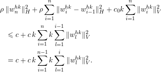 $$\begin{eqnarray}\displaystyle & & \displaystyle \unicode[STIX]{x1D70C}\,\Vert w_{n}^{hk}\Vert _{H}^{2}+\unicode[STIX]{x1D70C}\mathop{\sum }_{i=1}^{n}\Vert w_{i}^{hk}-w_{i-1}^{hk}\Vert _{H}^{2}+c_{0}k\mathop{\sum }_{i=1}^{n}\Vert w_{i}^{hk}\Vert _{V}^{2}\nonumber\\ \displaystyle & & \displaystyle \quad \leq c+c\,k\mathop{\sum }_{i=1}^{n}k\mathop{\sum }_{l=1}^{i-1}\Vert w_{l}^{hk}\Vert _{V}^{2}\nonumber\\ \displaystyle & & \displaystyle \quad =c+c\,k\mathop{\sum }_{i=1}^{n-1}k\mathop{\sum }_{l=1}^{i}\Vert w_{l}^{hk}\Vert _{V}^{2}.\end{eqnarray}$$
From (6.28), we have
 $$\begin{eqnarray}k\mathop{\sum }_{i=1}^{n}\Vert w_{i}^{hk}\Vert _{V}^{2}\leq c+c\,k\mathop{\sum }_{i=1}^{n-1}k\mathop{\sum }_{l=1}^{i}\Vert w_{l}^{hk}\Vert _{V}^{2},\quad 1\leq n\leq N.\end{eqnarray}$$
Apply Lemma 3.23 to get
 $$\begin{eqnarray}k\mathop{\sum }_{i=1}^{n}\Vert w_{i}^{hk}\Vert _{V}^{2}\leq c,\quad 1\leq n\leq N.\end{eqnarray}$$
By (6.28) again,
 $$\begin{eqnarray}\unicode[STIX]{x1D70C}\,\Vert w_{n}^{hk}\Vert _{H}^{2}+\unicode[STIX]{x1D70C}\mathop{\sum }_{i=1}^{n}\Vert w_{i}^{hk}-w_{i-1}^{hk}\Vert _{H}^{2}\leq c+c\,k\mathop{\sum }_{i=1}^{n-1}k\mathop{\sum }_{l=1}^{i}\Vert w_{l}^{hk}\Vert _{V}^{2}\leq c,\quad 1\leq n\leq N.\end{eqnarray}$$
Hence, (6.23) holds.◻
For error analysis, we additionally assume the Lipschitz continuity of the operator
 $A$
,
 $$\begin{eqnarray}\Vert Au-Av\Vert _{V^{\ast }}\leq L_{A}\Vert u-v\Vert _{V}\quad \text{for all}~u,v\in V,\end{eqnarray}$$
and assume the smoothness
 $$\begin{eqnarray}w\in H^{1}(0,T;V)\cap H^{2}(0,T;V^{\ast }),\quad q\in C^{1}([0,T]^{2};{\mathcal{L}}(V)).\end{eqnarray}$$
We start with an application of the strong monotonicity of
 $A$
:
 $$\begin{eqnarray}m_{A}\Vert w_{n}-w_{n}^{hk}\Vert _{V}^{2}\leq \langle A(w_{n})-A(w_{n}^{hk}),w_{n}-w_{n}^{hk}\rangle ,\end{eqnarray}$$
which can be rewritten as, for any
 $v^{h}\in V^{h}$
,
 $$\begin{eqnarray}\displaystyle m_{A}\Vert w_{n}-w_{n}^{hk}\Vert _{V}^{2} & \leq & \displaystyle \langle A(w_{n})-A(w_{n}^{hk}),w_{n}-v^{h}\rangle +\langle A(w_{n}),v^{h}-w_{n}\rangle \nonumber\\ \displaystyle & & \displaystyle +\,\langle A(w_{n}),w_{n}-w_{n}^{hk}\rangle +\langle A(w_{n}^{hk}),w_{n}^{hk}-v^{h}\rangle .\end{eqnarray}$$
By (6.1),
 $$\begin{eqnarray}\displaystyle & & \displaystyle \langle A(w_{n}),w_{n}-w_{n}^{hk}\rangle \nonumber\\ \displaystyle & & \displaystyle \quad \leq \langle \unicode[STIX]{x1D70C}\,{\dot{w}}_{n}+{\mathcal{S}}_{n}w,w_{n}^{hk}-w_{n}\rangle +j_{1}^{0}(\unicode[STIX]{x1D6FE}_{1}w_{n};\unicode[STIX]{x1D6FE}_{1}w_{n}^{hk}-\unicode[STIX]{x1D6FE}_{1}w_{n})\nonumber\\ \displaystyle & & \displaystyle \quad \quad +j_{2}^{0}(\unicode[STIX]{x1D6FE}_{2}w_{n};\unicode[STIX]{x1D6FE}_{2}w_{n}^{hk}-\unicode[STIX]{x1D6FE}_{2}w_{n})-\langle f_{n},w_{n}^{hk}-w_{n}\rangle .\end{eqnarray}$$
By (6.21),
 $$\begin{eqnarray}\displaystyle \langle A(w_{n}^{hk}),w_{n}^{hk}-v^{h}\rangle & \leq & \displaystyle \langle \unicode[STIX]{x1D70C}\,\displaystyle \frac{w_{n}^{hk}-w_{n-1}^{hk}}{k}+{\mathcal{S}}_{n}^{k}w^{hk},v^{h}-w_{n}^{hk}\rangle \nonumber\\ \displaystyle & & \displaystyle +\,j_{1}^{0}(\unicode[STIX]{x1D6FE}_{1}w_{n}^{hk};\unicode[STIX]{x1D6FE}_{1}v^{h}-\unicode[STIX]{x1D6FE}_{1}w_{n}^{hk})\nonumber\\ \displaystyle & & \displaystyle +\,j_{2}^{0}(\unicode[STIX]{x1D6FE}_{2}w_{n}^{hk};\unicode[STIX]{x1D6FE}_{2}v^{h}-\unicode[STIX]{x1D6FE}_{2}w_{n}^{hk})-\langle f_{n},v^{h}-w_{n}^{hk}\rangle .\end{eqnarray}$$
Use (6.32) and (6.33) in (6.31) to obtain
 $$\begin{eqnarray}\displaystyle m_{A}\Vert w_{n}-w_{n}^{hk}\Vert _{V}^{2} & \leq & \displaystyle \langle A(w_{n})-A(w_{n}^{hk}),w_{n}-v^{h}\rangle \nonumber\\ \displaystyle & & \displaystyle +\,R_{n}(v^{h}-w_{n})+\unicode[STIX]{x1D70C}\,I_{1}+I_{2}+I_{3},\end{eqnarray}$$
where
 $$\begin{eqnarray}\displaystyle R_{n}(v) & = & \displaystyle \langle \unicode[STIX]{x1D70C}\,{\dot{w}}_{n}+A(w_{n})+{\mathcal{S}}_{n}w-f_{n},v\rangle \nonumber\\ \displaystyle & & \displaystyle +\,j_{1}^{0}(\unicode[STIX]{x1D6FE}_{1}w_{n};\unicode[STIX]{x1D6FE}_{1}v)+j_{2}^{0}(\unicode[STIX]{x1D6FE}_{2}w_{n};\unicode[STIX]{x1D6FE}_{2}v),\quad v\in V\end{eqnarray}$$
is a residual-type term, and
 $$\begin{eqnarray}\displaystyle I_{1} & = & \displaystyle \langle {\dot{w}}_{n},w_{n}^{hk}-v^{h}\rangle +\langle \displaystyle \frac{w_{n}^{hk}-w_{n-1}^{hk}}{k},v^{h}-w_{n}^{hk}\rangle ,\end{eqnarray}$$
 $$\begin{eqnarray}\displaystyle I_{2} & = & \displaystyle \langle {\mathcal{S}}_{n}w-{\mathcal{S}}_{n}^{k}w^{hk},w_{n}^{hk}-v^{h}\rangle ,\end{eqnarray}$$
 $$\begin{eqnarray}\displaystyle I_{3} & = & \displaystyle j_{1}^{0}(\unicode[STIX]{x1D6FE}_{1}w_{n};\unicode[STIX]{x1D6FE}_{1}w_{n}^{hk}-\unicode[STIX]{x1D6FE}_{1}w_{n})+j_{1}^{0}(\unicode[STIX]{x1D6FE}_{1}w_{n}^{hk};\unicode[STIX]{x1D6FE}_{1}v^{h}-\unicode[STIX]{x1D6FE}_{1}w_{n}^{hk})\nonumber\\ \displaystyle & & \displaystyle -\,j_{1}^{0}(\unicode[STIX]{x1D6FE}_{1}w_{n};\unicode[STIX]{x1D6FE}_{1}v^{h}-\unicode[STIX]{x1D6FE}_{1}w_{n})+j_{2}^{0}(\unicode[STIX]{x1D6FE}_{2}w_{n};\unicode[STIX]{x1D6FE}_{2}w_{n}^{hk}-\unicode[STIX]{x1D6FE}_{2}w_{n})\nonumber\\ \displaystyle & & \displaystyle +\,j_{2}^{0}(\unicode[STIX]{x1D6FE}_{2}w_{n}^{hk};\unicode[STIX]{x1D6FE}_{2}v^{h}-\unicode[STIX]{x1D6FE}_{2}w_{n}^{hk})-j_{2}^{0}(\unicode[STIX]{x1D6FE}_{2}w_{n};\unicode[STIX]{x1D6FE}_{2}v^{h}-\unicode[STIX]{x1D6FE}_{2}w_{n}).\end{eqnarray}$$
In the following, we let
 $\unicode[STIX]{x1D716}>0$
be an arbitrarily fixed small positive number with its value to be chosen later. We will apply the modified Cauchy–Schwarz inequality (3.18) in several places, and the corresponding constant
 $c$
may depend on
 $\unicode[STIX]{x1D716}$
.
By the Lipschitz continuity of
 $A$
,
 $$\begin{eqnarray}\langle A(w_{n})-A(w_{n}^{hk}),w_{n}-v^{h}\rangle \leq L_{A}\Vert w_{n}-w_{n}^{hk}\Vert _{V}\Vert w_{n}-v^{h}\Vert _{V}.\end{eqnarray}$$
Apply (3.18) to get
 $$\begin{eqnarray}\langle A(w_{n})-A(w_{n}^{hk}),w_{n}-v^{h}\rangle \leq \unicode[STIX]{x1D716}\,\Vert w_{n}-w_{n}^{hk}\Vert _{V}^{2}+c\,\Vert w_{n}-v^{h}\Vert _{V}^{2}.\end{eqnarray}$$
To simplify the notation, we denote
 $$\begin{eqnarray}E_{n}={\dot{w}}_{n}-\displaystyle \frac{w_{n}-w_{n-1}}{k},\quad 1\leq n\leq N.\end{eqnarray}$$
Rewrite
 $I_{1}$
as
 $$\begin{eqnarray}\displaystyle I_{1} & = & \displaystyle -\langle \displaystyle \frac{(w_{n}-w_{n}^{hk})-(w_{n-1}-w_{n-1}^{hk})}{k},w_{n}-w_{n}^{hk}\rangle -\langle E_{n},w_{n}-w_{n}^{hk}\rangle \nonumber\\ \displaystyle & & \displaystyle +\,\langle \displaystyle \frac{(w_{n}-w_{n}^{hk})-(w_{n-1}-w_{n-1}^{hk})}{k},w_{n}-v^{h}\rangle +\langle E_{n},w_{n}-v^{h}\rangle .\nonumber\end{eqnarray}$$
Note that
 $$\begin{eqnarray}\displaystyle & & \displaystyle \langle \displaystyle \frac{(w_{n}-w_{n}^{hk})-(w_{n-1}-w_{n-1}^{hk})}{k},w_{n}-w_{n}^{hk}\rangle \nonumber\\ \displaystyle & & \displaystyle \quad \geq \displaystyle \frac{1}{2\,k}(\Vert w_{n}-w_{n}^{hk}\Vert _{H}^{2}-\Vert w_{n-1}-w_{n-1}^{hk}\Vert _{H}^{2}).\nonumber\end{eqnarray}$$
By (3.18),
 $$\begin{eqnarray}|\langle E_{n},w_{n}-w_{n}^{hk}\rangle |\leq \Vert E_{n}\Vert _{V^{\ast }}\Vert w_{n}-w_{n}^{hk}\Vert _{V}\leq \displaystyle \frac{\unicode[STIX]{x1D716}}{\unicode[STIX]{x1D70C}}\,\Vert w_{n}-w_{n}^{hk}\Vert _{V}^{2}+c\,\Vert E_{n}\Vert _{V^{\ast }}^{2}.\end{eqnarray}$$
Also,
 $$\begin{eqnarray}|\langle E_{n},w_{n}-v^{h}\rangle |\leq \Vert E_{n}\Vert _{V^{\ast }}\Vert w_{n}-v^{h}\Vert _{V}\leq \displaystyle \frac{1}{2}(\Vert E_{n}\Vert _{V^{\ast }}^{2}+\Vert w_{n}-v^{h}\Vert _{V}^{2}).\end{eqnarray}$$
Thus, we can bound
 $I_{1}$
as follows:
 $$\begin{eqnarray}\displaystyle I_{1} & \leq & \displaystyle -\displaystyle \frac{1}{2\,k}(\Vert w_{n}-w_{n}^{hk}\Vert _{H}^{2}-\Vert w_{n-1}-w_{n-1}^{hk}\Vert _{H}^{2})+\displaystyle \frac{\unicode[STIX]{x1D716}}{\unicode[STIX]{x1D70C}}\,\Vert w_{n}-w_{n}^{hk}\Vert _{V}^{2}\nonumber\\ \displaystyle & & \displaystyle +\,\langle \displaystyle \frac{(w_{n}-w_{n}^{hk})-(w_{n-1}-w_{n-1}^{hk})}{k},w_{n}-v^{h}\rangle \nonumber\\ \displaystyle & & \displaystyle +\,c\,\Vert E_{n}\Vert _{V^{\ast }}^{2}+c\,\Vert w_{n}-v^{h}\Vert _{V}^{2}.\end{eqnarray}$$
To bound the term
 $I_{2}$
, we write
 $$\begin{eqnarray}|I_{2}|\leq \Vert {\mathcal{S}}_{n}w-{\mathcal{S}}_{n}^{k}w^{hk}\Vert _{V^{\ast }}\Vert w_{n}^{hk}-v^{h}\Vert _{V}\end{eqnarray}$$
and note that
 $$\begin{eqnarray}\displaystyle \Vert {\mathcal{S}}_{n}w-{\mathcal{S}}_{n}^{k}w^{hk}\Vert _{V^{\ast }} & \leq & \displaystyle \Vert {\mathcal{S}}_{n}w-{\mathcal{S}}_{n}^{k}w\Vert _{V^{\ast }}+\Vert {\mathcal{S}}_{n}^{k}w-{\mathcal{S}}_{n}^{k}w^{hk}\Vert _{V^{\ast }},\nonumber\\ \displaystyle \Vert w_{n}^{hk}-v^{h}\Vert _{V} & \leq & \displaystyle \Vert w_{n}-v^{h}\Vert _{V}+\Vert w_{n}-w_{n}^{hk}\Vert _{V}.\nonumber\end{eqnarray}$$
Applying (3.18), we have
 $$\begin{eqnarray}\displaystyle |I_{2}| & \leq & \displaystyle \unicode[STIX]{x1D716}\,\Vert w_{n}-w_{n}^{hk}\Vert _{V}^{2}+c\,\Vert w_{n}-v^{h}\Vert _{V}^{2}\nonumber\\ \displaystyle & & \displaystyle +\,c\,\Vert {\mathcal{S}}_{n}^{k}w-{\mathcal{S}}_{n}^{k}w^{hk}\Vert _{V^{\ast }}^{2}+c\,\Vert {\mathcal{S}}_{n}w-{\mathcal{S}}_{n}^{k}w\Vert _{V^{\ast }}^{2}.\end{eqnarray}$$
By the definition of
 ${\mathcal{S}}^{k}$
, and assumptions on
 $G$
and
 $q$
, it is easy to see that
 $$\begin{eqnarray}\Vert {\mathcal{S}}_{n}^{k}w-{\mathcal{S}}_{n}^{k}w^{hk}\Vert _{V^{\ast }}\leq c\,k\mathop{\sum }_{i=0}^{n-1}\Vert w_{i}-w_{i}^{hk}\Vert _{V}.\end{eqnarray}$$
As in the derivation of (5.26), for
 ${\mathcal{S}}$
and
 ${\mathcal{S}}^{k}$
defined by (6.18) and (6.19), we have the bound
 $$\begin{eqnarray}\Vert {\mathcal{S}}_{n}w-{\mathcal{S}}_{n}^{k}w\Vert _{V^{\ast }}\leq c\,k\,\Vert w\Vert _{H^{1}(0,T;V)}.\end{eqnarray}$$
Use (6.43) and (6.44) in (6.42) to obtain
 $$\begin{eqnarray}\displaystyle |I_{2}| & \leq & \displaystyle \unicode[STIX]{x1D716}\,\Vert w_{n}-w_{n}^{hk}\Vert _{V}^{2}+c\,\Vert w_{n}-v^{h}\Vert _{V}^{2}\nonumber\\ \displaystyle & & \displaystyle +\,c\,k^{2}\Vert w\Vert _{H^{1}(0,T;V)}^{2}+c\,k\mathop{\sum }_{i=0}^{n-1}\Vert w_{i}-w_{i}^{hk}\Vert _{V}^{2}.\end{eqnarray}$$
To bound
 $I_{3}$
, we first apply the subadditivity of the generalized directional derivative, with
 $l=1,2$
,
 $$\begin{eqnarray}\displaystyle j_{l}^{0}(\unicode[STIX]{x1D6FE}_{l}w_{n}^{hk};\unicode[STIX]{x1D6FE}_{l}v^{h}-\unicode[STIX]{x1D6FE}_{l}w_{n}^{hk}) & \leq & \displaystyle j_{l}^{0}(\unicode[STIX]{x1D6FE}_{l}w_{n}^{hk};\unicode[STIX]{x1D6FE}_{l}w_{n}-\unicode[STIX]{x1D6FE}_{l}w_{n}^{hk})\nonumber\\ \displaystyle & & \displaystyle +\,j_{l}^{0}(\unicode[STIX]{x1D6FE}_{l}w_{n}^{hk};\unicode[STIX]{x1D6FE}_{l}v^{h}-\unicode[STIX]{x1D6FE}_{l}w_{n}),\nonumber\end{eqnarray}$$
and then apply the relaxed monotonicity,
 $$\begin{eqnarray}j_{l}^{0}(\unicode[STIX]{x1D6FE}_{l}w_{n};\unicode[STIX]{x1D6FE}_{l}w_{n}^{hk}-\unicode[STIX]{x1D6FE}_{l}w_{n})+j_{l}^{0}(\unicode[STIX]{x1D6FE}_{l}w_{n}^{hk};\unicode[STIX]{x1D6FE}_{l}w_{n}-\unicode[STIX]{x1D6FE}_{l}w_{n}^{hk})\leq \unicode[STIX]{x1D6FC}_{l}c_{j}^{2}\Vert w_{n}-w_{n}^{hk}\Vert _{V}^{2}.\end{eqnarray}$$
As a result,
 $$\begin{eqnarray}\displaystyle I_{3} & \leq & \displaystyle (\unicode[STIX]{x1D6FC}_{1}c_{1}^{2}+\unicode[STIX]{x1D6FC}_{2}c_{2}^{2})\Vert w_{n}-w_{n}^{hk}\Vert _{V}^{2}\nonumber\\ \displaystyle & & \displaystyle +\,j_{1}^{0}(\unicode[STIX]{x1D6FE}_{1}w_{n}^{hk};\unicode[STIX]{x1D6FE}_{1}v^{h}-\unicode[STIX]{x1D6FE}_{1}w_{n})-j_{1}^{0}(\unicode[STIX]{x1D6FE}_{1}w_{n};\unicode[STIX]{x1D6FE}_{1}v^{h}-\unicode[STIX]{x1D6FE}_{1}w_{n})\nonumber\\ \displaystyle & & \displaystyle +\,j_{2}^{0}(\unicode[STIX]{x1D6FE}_{2}w_{n}^{hk};\unicode[STIX]{x1D6FE}_{2}v^{h}-\unicode[STIX]{x1D6FE}_{2}w_{n})-j_{2}^{0}(\unicode[STIX]{x1D6FE}_{2}w_{n};\unicode[STIX]{x1D6FE}_{2}v^{h}-\unicode[STIX]{x1D6FE}_{2}w_{n}).\nonumber\end{eqnarray}$$
By the assumption on
 $j_{l}$
,
 $$\begin{eqnarray}\displaystyle |j_{l}^{0}(\unicode[STIX]{x1D6FE}_{l}w_{n}^{hk};\unicode[STIX]{x1D6FE}_{l}v^{h}-\unicode[STIX]{x1D6FE}_{l}w_{n})| & \leq & \displaystyle (c_{0l}+c_{1l}\Vert \unicode[STIX]{x1D6FE}_{l}w_{n}^{hk}\Vert _{V_{l}})\Vert \unicode[STIX]{x1D6FE}_{l}(w_{n}-v^{h})\Vert _{V_{l}},\nonumber\\ \displaystyle |j_{l}^{0}(\unicode[STIX]{x1D6FE}_{l}w_{n};\unicode[STIX]{x1D6FE}_{l}v^{h}-\unicode[STIX]{x1D6FE}_{l}w_{n})| & \leq & \displaystyle (c_{0l}+c_{1l}\Vert \unicode[STIX]{x1D6FE}_{l}w_{n}\Vert _{V_{l}})\Vert \unicode[STIX]{x1D6FE}_{l}(w_{n}-v^{h})\Vert _{V_{l}}.\nonumber\end{eqnarray}$$
Since
 $\Vert \unicode[STIX]{x1D6FE}_{l}w_{n}\Vert _{V_{l}}$
is uniformly bounded, we conclude that there is a constant
 $c$
such that
 $$\begin{eqnarray}\displaystyle I_{3} & \leq & \displaystyle (\unicode[STIX]{x1D6FC}_{1}c_{1}^{2}+\unicode[STIX]{x1D6FC}_{2}c_{2}^{2})\Vert w_{n}-w_{n}^{hk}\Vert _{V}^{2}\nonumber\\ \displaystyle & & \displaystyle +\,c(1+\Vert w_{n}^{hk}\Vert _{V})(\Vert \unicode[STIX]{x1D6FE}_{1}(w_{n}-v^{h})\Vert _{V_{1}}+\Vert \unicode[STIX]{x1D6FE}_{2}(w_{n}-v^{h})\Vert _{V_{2}}).\end{eqnarray}$$
Denote the error
 $$\begin{eqnarray}e_{n}=w_{n}-w_{n}^{hk},\quad 0\leq n\leq N.\end{eqnarray}$$
Then, by applying (6.39), (6.41), (6.45) and (6.46) in (6.34), we have
 $$\begin{eqnarray}\displaystyle & & \displaystyle \displaystyle \frac{\unicode[STIX]{x1D70C}}{2\,k}(\Vert e_{n}\Vert _{H}^{2}-\Vert e_{n-1}\Vert _{H}^{2})+(m_{A}-\unicode[STIX]{x1D6FC}_{1}c_{1}^{2}-\unicode[STIX]{x1D6FC}_{2}c_{2}^{2}-3\,\unicode[STIX]{x1D716})\Vert e_{n}\Vert _{V}^{2}\nonumber\\ \displaystyle & & \displaystyle \quad \leq c(\Vert w_{n}-v^{h}\Vert _{V}^{2}+|R_{n}(v^{h}-w_{n})|+\Vert E_{n}\Vert _{V^{\ast }}^{2})+c\,k^{2}\Vert w\Vert _{H^{1}(0,T;V)}^{2}\nonumber\\ \displaystyle & & \displaystyle \quad \quad +c(1+\Vert w_{n}^{hk}\Vert _{V})(\Vert \unicode[STIX]{x1D6FE}_{1}(w_{n}-v^{h})\Vert _{V_{1}}+\Vert \unicode[STIX]{x1D6FE}_{2}(w_{n}-v^{h})\Vert _{V_{2}})\nonumber\\ \displaystyle & & \displaystyle \quad \quad +\langle \unicode[STIX]{x1D70C}\,\displaystyle \frac{e_{n}-e_{n-1}}{k},w_{n}-v^{h}\rangle +c\,k\mathop{\sum }_{i=0}^{n-1}\Vert e_{i}\Vert _{V}^{2}.\end{eqnarray}$$
Applying the smallness condition
 $\unicode[STIX]{x1D6FC}_{1}c_{1}^{2}+\unicode[STIX]{x1D6FC}_{2}c_{2}^{2}<m_{A}$
from (6.5) and choosing
 $\unicode[STIX]{x1D716}=(m_{A}-\unicode[STIX]{x1D6FC}_{1}c_{1}^{2}-\unicode[STIX]{x1D6FC}_{2}c_{2}^{2})/6$
, we derive from (6.48) the following inequality, with
 $v^{h}\in V^{h}$
renamed as
 $v_{n}^{h}\in V^{h}$
,
 $$\begin{eqnarray}\displaystyle & & \displaystyle \Vert e_{n}\Vert _{H}^{2}-\Vert e_{n-1}\Vert _{H}^{2}+k\,\Vert e_{n}\Vert _{V}^{2}\nonumber\\ \displaystyle & & \displaystyle \quad \leq c\,k(\Vert w_{n}-v_{n}^{h}\Vert _{V}^{2}+|R_{n}(v_{n}^{h}-w_{n})|+\Vert E_{n}\Vert _{V^{\ast }}^{2})+c\,k^{3}\Vert w\Vert _{H^{1}(0,T;V)}^{2}\nonumber\\ \displaystyle & & \displaystyle \quad \quad +c\,k(1+\Vert w_{n}^{hk}\Vert _{V})(\Vert \unicode[STIX]{x1D6FE}_{1}(w_{n}-v_{n}^{h})\Vert _{V_{1}}+\Vert \unicode[STIX]{x1D6FE}_{2}(w_{n}-v_{n}^{h})\Vert _{V_{2}})\nonumber\\ \displaystyle & & \displaystyle \quad \quad +c\,\langle e_{n}-e_{n-1},w_{n}-v_{n}^{h}\rangle +c\,k^{2}\mathop{\sum }_{i=0}^{n-1}\Vert e_{i}\Vert _{V}^{2}.\end{eqnarray}$$
We replace
 $n$
with
 $i$
in (6.49) and make a summation over
 $i$
from
 $1$
to
 $n$
,
 $$\begin{eqnarray}\displaystyle & & \displaystyle \Vert e_{n}\Vert _{H}^{2}-\Vert e_{0}\Vert _{H}^{2}+k\mathop{\sum }_{i=1}^{n}\Vert e_{i}\Vert _{V}^{2}\nonumber\\ \displaystyle & & \displaystyle \quad \leq c\,k\mathop{\sum }_{i=1}^{n}(\Vert w_{i}-v_{i}^{h}\Vert _{V}^{2}+|R_{i}(v_{i}^{h}-w_{i})|+\Vert E_{i}\Vert _{V^{\ast }}^{2})+c\,k^{2}\Vert w\Vert _{H^{1}(0,T;V)}^{2}\nonumber\\ \displaystyle & & \displaystyle \quad \quad +c\,k\mathop{\sum }_{i=1}^{n}(1+\Vert w_{i}^{hk}\Vert _{V})(\Vert \unicode[STIX]{x1D6FE}_{1}(w_{i}-v_{i}^{h})\Vert _{V_{1}}+\Vert \unicode[STIX]{x1D6FE}_{2}(w_{i}-v_{i}^{h})\Vert _{V_{2}})\nonumber\\ \displaystyle & & \displaystyle \quad \quad +c\,k\mathop{\sum }_{i=1}^{n}\langle e_{i}-e_{i-1},w_{i}-v_{i}^{h}\rangle +c\,k\mathop{\sum }_{i=0}^{n-1}k\mathop{\sum }_{l=0}^{i}\Vert e_{l}\Vert _{V}^{2}.\end{eqnarray}$$
Now
 $$\begin{eqnarray}\displaystyle & & \displaystyle \mathop{\sum }_{i=1}^{n}(1+\Vert w_{i}^{hk}\Vert _{V})(\Vert \unicode[STIX]{x1D6FE}_{1}(w_{i}-v_{i}^{h})\Vert _{V_{1}}+\Vert \unicode[STIX]{x1D6FE}_{2}(w_{i}-v_{i}^{h})\Vert _{V_{2}})\nonumber\\ \displaystyle & & \displaystyle \quad \leq \left[\mathop{\sum }_{i=1}^{n}(1+\Vert w_{i}^{hk}\Vert _{V})^{2}\right]^{1/2}\left[\mathop{\sum }_{i=1}^{n}(\Vert \unicode[STIX]{x1D6FE}_{1}(w_{i}-v_{i}^{h})\Vert _{V_{1}}+\Vert \unicode[STIX]{x1D6FE}_{2}(w_{i}-v_{i}^{h})\Vert _{V_{2}})^{2}\right]^{1/2}.\nonumber\end{eqnarray}$$
By Proposition 6.4,
 $k\sum _{i=1}^{n}(1+\Vert w_{i}^{hk}\Vert _{V})^{2}$
is uniformly bounded. Thus,
 $$\begin{eqnarray}\displaystyle & & \displaystyle c\,k\mathop{\sum }_{i=1}^{n}(1+\Vert w_{i}^{hk}\Vert _{V})(\Vert \unicode[STIX]{x1D6FE}_{1}(w_{i}-v_{i}^{h})\Vert _{V_{1}}+\Vert \unicode[STIX]{x1D6FE}_{2}(w_{i}-v_{i}^{h})\Vert _{V_{2}})\nonumber\\ \displaystyle & & \displaystyle \quad \leq c\left[k\mathop{\sum }_{i=1}^{n}(\Vert \unicode[STIX]{x1D6FE}_{1}(w_{i}-v_{i}^{h})\Vert _{V_{1}}^{2}+\Vert \unicode[STIX]{x1D6FE}_{2}(w_{i}-v_{i}^{h})\Vert _{V_{2}}^{2})\right]^{1/2}.\nonumber\end{eqnarray}$$
Write
 $$\begin{eqnarray}\displaystyle \mathop{\sum }_{i=1}^{n}\langle e_{i}-e_{i-1},w_{i}-v_{i}^{h}\rangle & = & \displaystyle \mathop{\sum }_{i=1}^{n}\langle e_{i},w_{i}-v_{i}^{h}\rangle -\mathop{\sum }_{i=0}^{n-1}\langle e_{i},w_{i+1}-v_{i+1}^{h}\rangle \nonumber\\ \displaystyle & = & \displaystyle \langle e_{n},w_{n}-v_{n}^{h}\rangle \nonumber\\ \displaystyle & & \displaystyle \quad +\mathop{\sum }_{i=1}^{n-1}\langle e_{i},(w_{i}-v_{i}^{h})-(w_{i+1}-v_{i+1}^{h})\rangle \nonumber\\ \displaystyle & & \displaystyle \quad -\langle e_{0},w_{1}-v_{1}^{h}\rangle \nonumber\end{eqnarray}$$
and we bound the terms on the right-hand side as follows. For the first term, with a small
 $\unicode[STIX]{x1D716}_{0}>0$
,
 $$\begin{eqnarray}|\langle e_{n},w_{n}-v_{n}^{h}\rangle |\leq \Vert e_{n}\Vert _{H}\Vert w_{n}-v_{n}^{h}\Vert _{H}\leq \unicode[STIX]{x1D716}_{0}\Vert e_{n}\Vert _{H}^{2}+c\,\Vert w_{n}-v_{n}^{h}\Vert _{H}^{2}.\end{eqnarray}$$
For the second term,
 $$\begin{eqnarray}\displaystyle & & \displaystyle |\langle e_{i},(w_{i}-v_{i}^{h})-(w_{i+1}-v_{i+1}^{h})\rangle |\nonumber\\ \displaystyle & & \displaystyle \quad \leq \Vert e_{i}\Vert _{H}\Vert (w_{i}-v_{i}^{h})-(w_{i+1}-v_{i+1}^{h})\Vert _{H}\nonumber\\ \displaystyle & & \displaystyle \quad \leq \displaystyle \frac{k}{2}(\Vert e_{i}\Vert _{H}^{2}+k^{-2}\Vert (w_{i}-v_{i}^{h})-(w_{i+1}-v_{i+1}^{h})\Vert _{H}^{2}).\nonumber\end{eqnarray}$$
For the last term,
 $$\begin{eqnarray}|\langle e_{0},w_{1}-v_{1}^{h}\rangle |\leq \Vert e_{0}\Vert _{H}\Vert w_{1}-v_{1}^{h}\Vert _{H}\leq \displaystyle \frac{1}{2}(\Vert e_{0}\Vert _{H}^{2}+\Vert w_{1}-v_{1}^{h}\Vert _{H}^{2}).\end{eqnarray}$$
For the term
 $E_{n}$
defined by (6.40), we can write
 $$\begin{eqnarray}E_{n}=\displaystyle \frac{1}{k}\int _{t_{n-1}}^{t_{n}}(t-t_{n-1})\ddot{w}(t)\,\text{d}t.\end{eqnarray}$$
Thus, we have the upper bound
 $$\begin{eqnarray}\Vert E_{n}\Vert _{V^{\ast }}\leq \Vert \ddot{w}\Vert _{L^{1}(t_{n-1},t_{n};V^{\ast })}\end{eqnarray}$$
and then
 $$\begin{eqnarray}\mathop{\sum }_{i=1}^{n}\Vert E_{i}\Vert _{V^{\ast }}^{2}\leq \mathop{\sum }_{i=1}^{n}\Vert \ddot{w}\Vert _{L^{1}(t_{i-1},t_{i};V^{\ast })}^{2}\leq k\,\Vert \ddot{w}\Vert _{L^{2}(0,T;V^{\ast })}^{2}.\end{eqnarray}$$
Using the above inequalities with
 $\unicode[STIX]{x1D716}_{0}>0$
sufficiently small, we derive from (6.50) that
 $$\begin{eqnarray}\displaystyle \Vert e_{n}\Vert _{H}^{2}+k\mathop{\sum }_{i=1}^{n}\Vert e_{i}\Vert _{V}^{2} & \leq & \displaystyle c\,k\mathop{\sum }_{i=1}^{n}(\Vert w_{i}-v_{i}^{h}\Vert ^{2}+|R_{i}(v_{i}^{h}-w_{i})|)\nonumber\\ \displaystyle & & \displaystyle \quad ~~+c\,k^{2}(\Vert \ddot{w}\Vert _{L^{2}(0,T;V^{\ast })}^{2}+\Vert w\Vert _{H^{1}(0,T;V)}^{2})\nonumber\\ \displaystyle & & \displaystyle \quad ~~+c\left[k\mathop{\sum }_{i=1}^{n}(\Vert \unicode[STIX]{x1D6FE}_{1}(w_{i}-v_{i}^{h})\Vert _{V_{1}}^{2}+\Vert \unicode[STIX]{x1D6FE}_{2}(w_{i}-v_{i}^{h})\Vert _{V_{2}}^{2})\right]^{1/2}\nonumber\\ \displaystyle & & \displaystyle \quad ~~+c\,k^{-1}\mathop{\sum }_{i=1}^{n-1}\Vert (w_{i}-v_{i}^{h})-(w_{i+1}-v_{i+1}^{h})\Vert _{H}^{2}\nonumber\\ \displaystyle & & \displaystyle \quad ~~+c(\Vert e_{0}\Vert _{H}^{2}+k\,\Vert e_{0}\Vert _{V}^{2}+\Vert w_{1}-v_{1}^{h}\Vert _{H}^{2}+\Vert w_{n}-v_{n}^{h}\Vert _{H}^{2})\nonumber\\ \displaystyle & & \displaystyle \quad ~~+c\,k\mathop{\sum }_{i=0}^{n-1}\biggl(\Vert e_{i}\Vert _{H}^{2}+k\mathop{\sum }_{l=1}^{i}\Vert e_{l}\Vert _{V}^{2}\biggr),\quad 1\leq n\leq N.\nonumber\end{eqnarray}$$
We then apply Lemma 3.23 to find that
 $$\begin{eqnarray}\displaystyle \max _{1\leq n\leq N}\Vert e_{n}\Vert _{H}^{2}+k\mathop{\sum }_{n=1}^{N}\Vert e_{n}\Vert _{V}^{2} & \leq & \displaystyle c\,k^{2}(\Vert \ddot{w}\Vert _{L^{2}(0,T;V^{\ast })}^{2}+\Vert w\Vert _{H^{1}(0,T;V)}^{2})\nonumber\\ \displaystyle & & \displaystyle \quad +c(\Vert e_{0}\Vert _{H}^{2}+k\,\Vert e_{0}\Vert _{V}^{2})+c\,\max _{1\leq n\leq N}\tilde{E}_{n},\end{eqnarray}$$
where
 $$\begin{eqnarray}\displaystyle \tilde{E}_{n} & = & \displaystyle \inf _{v_{i}^{h}\in V^{h},\,1\leq i\leq n}\bigg\{k\mathop{\sum }_{i=1}^{n}(\Vert w_{i}-v_{i}^{h}\Vert _{V}^{2}+|R_{i}(v_{i}^{h}-w_{i})|)\nonumber\\ \displaystyle & & \displaystyle \quad +\biggl[k\mathop{\sum }_{i=1}^{n}(\Vert \unicode[STIX]{x1D6FE}_{1}(w_{i}-v_{i}^{h})\Vert _{V_{1}}^{2}+\Vert \unicode[STIX]{x1D6FE}_{2}(w_{i}-v_{i}^{h})\Vert _{V_{2}}^{2})\biggr]^{1/2}\nonumber\\ \displaystyle & & \displaystyle \quad +k^{-1}\mathop{\sum }_{i=1}^{n-1}\Vert (w_{i}-v_{i}^{h})-(w_{i+1}-v_{i+1}^{h})\Vert _{V^{\ast }}^{2}\nonumber\\ \displaystyle & & \displaystyle \quad +\Vert w_{1}-v_{1}^{h}\Vert _{H}^{2}+\Vert w_{n}-v_{n}^{h}\Vert _{H}^{2}\bigg\}.\end{eqnarray}$$
Summarizing, we state the result in the form of a theorem.
Theorem 6.5. Keep the assumptions of Theorem 6.2, and assume further that (6.17), (6.18), (6.19), (6.29) and (6.30) hold. Then for the numerical solution
 $w^{hk}=\{w_{n}^{hk_{}^{}\}}\subset V^{h}$
defined by Problem 6.3, we have the inequality
 $$\begin{eqnarray}\displaystyle & & \displaystyle \max _{1\leq n\leq N}\Vert w_{n}-w_{n}^{hk}\Vert _{H}^{2}+k\mathop{\sum }_{n=1}^{N}\Vert w_{n}-w_{n}^{hk}\Vert _{V}^{2}\nonumber\\ \displaystyle & & \displaystyle \quad \leq c\,k^{2}(\Vert \ddot{w}\Vert _{L^{2}(0,T;V^{\ast })}^{2}+\Vert w\Vert _{H^{1}(0,T;V)}^{2})\nonumber\\ \displaystyle & & \displaystyle \quad \quad +c(\Vert w_{0}-w_{0}^{h}\Vert _{H}^{2}+k\,\Vert w_{0}-w_{0}^{h}\Vert _{V}^{2})+c\,\max _{1\leq n\leq N}\tilde{E}_{n},\end{eqnarray}$$
where
 $\tilde{E}_{n}$
is defined by (6.52).
The inequality (6.53) will be the starting point for concrete error estimation of numerical solutions for Problem 2.10 in Section 9.2.
We comment that for the approximate operator
 ${\mathcal{S}}^{k}$
, instead of (6.19), we can also use (5.33) or define
 $$\begin{eqnarray}{\mathcal{S}}_{n}^{k}w^{hk}=G\biggl(k\mathop{\sum }_{i=1}^{n}q(t_{n},t_{i})\,w_{i}^{hk}+a_{{\mathcal{S}}}\biggr),\quad 1\leq n\leq N,\end{eqnarray}$$
for any
 $w^{hk}=\{w_{i}^{hk_{}^{}\}}\subset V^{h}$
. For both these choices, the error bound (6.53) is still valid for
 $k$
small.
7 Studies of the static contact problem
In this section we study the static contact problem, Problem 2.6. We first explore the solution existence and uniqueness, then introduce a linear finite element method to solve the problem and derive an optimal order error estimate under certain solution regularity assumptions. Finally, we present numerical simulation results.
7.1 Existence and uniqueness
We start with an existence and uniqueness result for Problem 2.6. In addition to the space
 $V$
defined in (2.3), we introduce the spaces
 $$\begin{eqnarray}\displaystyle V_{\unicode[STIX]{x1D711}} & = & \displaystyle L^{2}(\unicode[STIX]{x1D6E4}_{3})^{d},\end{eqnarray}$$
 $$\begin{eqnarray}\displaystyle V_{j} & = & \displaystyle L^{2}(\unicode[STIX]{x1D6E4}_{3}).\end{eqnarray}$$
Let
 $\unicode[STIX]{x1D706}_{1}>0$
be the smallest eigenvalue of the eigenvalue problem
 $$\begin{eqnarray}\boldsymbol{u}\in V,\quad \int _{\unicode[STIX]{x1D6FA}}\unicode[STIX]{x1D73A}(\boldsymbol{u})\cdot \unicode[STIX]{x1D73A}(\boldsymbol{v})\,\text{d}x=\unicode[STIX]{x1D706}\int _{\unicode[STIX]{x1D6E4}_{3}}\boldsymbol{u}\cdot \boldsymbol{v}\,\text{d}a\quad \text{for all}~\boldsymbol{v}\in V\end{eqnarray}$$
and let
 $\unicode[STIX]{x1D706}_{1\unicode[STIX]{x1D708}}>0$
be the smallest eigenvalue of the eigenvalue problem
 $$\begin{eqnarray}\boldsymbol{u}\in V,\quad \int _{\unicode[STIX]{x1D6FA}}\unicode[STIX]{x1D73A}(\boldsymbol{u})\cdot \unicode[STIX]{x1D73A}(\boldsymbol{v})\,\text{d}x=\unicode[STIX]{x1D706}\int _{\unicode[STIX]{x1D6E4}_{3}}u_{\unicode[STIX]{x1D708}}v_{\unicode[STIX]{x1D708}}\,\text{d}a\quad \text{for all}~\boldsymbol{v}\in V.\end{eqnarray}$$
It is easy to check that
 $$\begin{eqnarray}\displaystyle & & \displaystyle \unicode[STIX]{x1D706}_{1}=\inf \big\{\Vert \unicode[STIX]{x1D73A}(\boldsymbol{v})\Vert _{L^{2}(\unicode[STIX]{x1D6FA};\mathbb{S}^{d})}^{2}\mid \boldsymbol{v}\in V,\,\Vert \boldsymbol{v}\Vert _{L^{2}(\unicode[STIX]{x1D6E4}_{3};\mathbb{R}^{d})}=1\big\},\nonumber\\ \displaystyle & & \displaystyle \unicode[STIX]{x1D706}_{1\unicode[STIX]{x1D708}}=\inf \big\{\Vert \unicode[STIX]{x1D73A}(\boldsymbol{v})\Vert _{L^{2}(\unicode[STIX]{x1D6FA};\mathbb{S}^{d})}^{2}\mid \boldsymbol{v}\in V,\,\Vert v_{\unicode[STIX]{x1D708}}\Vert _{L^{2}(\unicode[STIX]{x1D6E4}_{3})}=1\big\},\nonumber\end{eqnarray}$$
and both values exist and are positive.
Theorem 7.1. Assume (2.34)–(2.38) and
 $$\begin{eqnarray}L_{F_{b}}\unicode[STIX]{x1D706}_{1}^{-1}+\unicode[STIX]{x1D6FC}_{j_{\unicode[STIX]{x1D708}}}\unicode[STIX]{x1D706}_{1\unicode[STIX]{x1D708}}^{-1}<m_{{\mathcal{F}}}.\end{eqnarray}$$
Then Problem 2.6 has a unique solution.
Proof. We apply Theorem 4.4 with
 $X=V$
,
 $X_{\unicode[STIX]{x1D711}}=V_{\unicode[STIX]{x1D711}}$
of (7.1),
 $X_{j}=V_{j}$
of (7.2),
 $K=U$
,
 $\unicode[STIX]{x1D6FE}_{\unicode[STIX]{x1D711}}:V\rightarrow V_{\unicode[STIX]{x1D711}}$
being the trace operator,
 $\unicode[STIX]{x1D6FE}_{j}:V\rightarrow V_{j}$
being the normal trace operator, and
 $A:V\rightarrow V^{\ast }$
,
 $\unicode[STIX]{x1D711}:V_{\unicode[STIX]{x1D711}}\times V_{\unicode[STIX]{x1D711}}\rightarrow \mathbb{R}$
,
 $j:V_{j}\rightarrow \mathbb{R}$
and
 $\boldsymbol{f}\in V^{\ast }$
defined by
 $$\begin{eqnarray}\displaystyle \langle A\boldsymbol{u},\boldsymbol{v}\rangle & = & \displaystyle \int _{\unicode[STIX]{x1D6FA}}{\mathcal{F}}\unicode[STIX]{x1D73A}(\boldsymbol{u})\cdot \unicode[STIX]{x1D73A}(\boldsymbol{v})\,\text{d}x,\quad \boldsymbol{u},\boldsymbol{v}\in V,\end{eqnarray}$$
 $$\begin{eqnarray}\displaystyle \unicode[STIX]{x1D711}(\boldsymbol{z}_{1},\boldsymbol{z}_{2}) & = & \displaystyle \int _{\unicode[STIX]{x1D6E4}_{3}}F_{b}(z_{1,\unicode[STIX]{x1D708}})\,\Vert \boldsymbol{z}_{2,\unicode[STIX]{x1D70F}}\Vert \,\text{d}a,\quad \boldsymbol{z}_{1},\boldsymbol{z}_{2}\in V_{\unicode[STIX]{x1D711}},\end{eqnarray}$$
 $$\begin{eqnarray}\displaystyle j(z) & = & \displaystyle \int _{\unicode[STIX]{x1D6E4}_{3}}j_{\unicode[STIX]{x1D708}}(z)\,\text{d}a,\quad z\in V_{j},\end{eqnarray}$$
 $$\begin{eqnarray}\displaystyle \langle \boldsymbol{f},\boldsymbol{v}\rangle & = & \displaystyle \int _{\unicode[STIX]{x1D6FA}}\boldsymbol{f}_{0}\cdot \boldsymbol{v}\,\text{d}x+\int _{\unicode[STIX]{x1D6E4}_{2}}\boldsymbol{f}_{2}\cdot \boldsymbol{v}\,\text{d}a,\quad \boldsymbol{v}\in V.\end{eqnarray}$$
Here and below, for any vector field
 $\boldsymbol{z}_{i}$
we use the notation
 $z_{i,\unicode[STIX]{x1D708}}$
and
 $\boldsymbol{z}_{i,\unicode[STIX]{x1D70F}}$
to represent its normal and tangential components, respectively. Observe that (4.16) holds with
 $c_{\unicode[STIX]{x1D711}}=\unicode[STIX]{x1D706}_{1}^{-1/2}$
, (4.17) holds with
 $c_{j}=\unicode[STIX]{x1D706}_{1\unicode[STIX]{x1D708}}^{-1/2}$
.
Then, (4.1) is obviously true: the set is non-empty since the zero function belongs to
 $U$
. The operator
 $A$
defined by (7.6) satisfies condition (4.2) with
 $m_{A}=m_{{\mathcal{F}}}$
and condition (4.47) with
 $L_{A}=L_{{\mathcal{F}}}$
. Indeed, for
 $\boldsymbol{u},\boldsymbol{v},\boldsymbol{w}\in V$
, by assumption (2.34(a)), we have
 $$\begin{eqnarray}\langle A\boldsymbol{u}-A\boldsymbol{v},\boldsymbol{w}\rangle \leq ({\mathcal{F}}\unicode[STIX]{x1D73A}(\boldsymbol{u})-{\mathcal{F}}\unicode[STIX]{x1D73A}(\boldsymbol{v}),\unicode[STIX]{x1D73A}(\boldsymbol{w}))_{Q}\leq L_{{\mathcal{F}}}\Vert \boldsymbol{u}-\boldsymbol{v}\Vert _{V}\Vert \boldsymbol{w}\Vert _{V}.\end{eqnarray}$$
Thus,
 $$\begin{eqnarray}\Vert A\boldsymbol{u}-A\boldsymbol{v}\Vert _{V^{\ast }}\leq L_{{\mathcal{F}}}\Vert \boldsymbol{u}-\boldsymbol{v}\Vert _{V}\quad \text{for all}~\boldsymbol{u},\boldsymbol{v}\in V.\end{eqnarray}$$
This shows that
 $A$
is Lipschitz continuous. On the other hand,
 $$\begin{eqnarray}\langle A\boldsymbol{u}-A\boldsymbol{v},\boldsymbol{u}-\boldsymbol{v}\rangle =({\mathcal{F}}\unicode[STIX]{x1D73A}(\boldsymbol{u})-{\mathcal{F}}\unicode[STIX]{x1D73A}(\boldsymbol{v}),\unicode[STIX]{x1D73A}(\boldsymbol{u})-\unicode[STIX]{x1D73A}(\boldsymbol{v}))_{Q}.\end{eqnarray}$$
Then, assumption (2.34(b)) yields
 $$\begin{eqnarray}\langle A\boldsymbol{u}-A\boldsymbol{v},\boldsymbol{u}-\boldsymbol{v}\rangle \geq m_{{\mathcal{F}}}\Vert \boldsymbol{u}-\boldsymbol{v}\Vert _{V}^{2}\quad \text{for all}~\boldsymbol{u},\boldsymbol{v}\in V.\end{eqnarray}$$
This shows that condition (4.2(b)) is satisfied with
 $m_{A}=m_{{\mathcal{F}}}$
. Since
 $A$
is Lipschitz continuous it follows that
 $A$
is bounded and hemicontinuous, that is, (4.2(a)) holds.
Next, for
 $\unicode[STIX]{x1D711}$
defined by (7.7), it is easy to check that assumption (2.36) implies (4.18) with
 $\unicode[STIX]{x1D6FC}_{\unicode[STIX]{x1D711}}=L_{F_{b}}$
. On the other hand, hypothesis (2.35) allows us to apply a variant of Theorem 3.47 in Migórski, Ochal and Sofonea (Reference Migórski, Ochal and Sofonea2013). In this way we deduce that the function
 $j$
given by (7.8) satisfies (4.19) with
 $c_{0}=\sqrt{2\,\operatorname{meas}\,(\unicode[STIX]{x1D6E4}_{3})}\,\bar{c}_{0}$
,
 $c_{1}=\sqrt{2}\,\bar{c}_{1}$
and
 $\unicode[STIX]{x1D6FC}_{j}=\unicode[STIX]{x1D6FC}_{j_{\unicode[STIX]{x1D708}}}$
. Moreover,
 $$\begin{eqnarray}j^{0}(\unicode[STIX]{x1D6FE}_{j}\boldsymbol{u};\unicode[STIX]{x1D6FE}_{j}\boldsymbol{v})\leq \int _{\unicode[STIX]{x1D6E4}_{3}}j_{\unicode[STIX]{x1D708}}^{0}(\boldsymbol{x},u_{\unicode[STIX]{x1D708}}(\boldsymbol{x});v_{\unicode[STIX]{x1D708}}(\boldsymbol{x}))\,\text{d}a\quad \text{for all}~\boldsymbol{u},\boldsymbol{v}\in V.\end{eqnarray}$$
This implies (4.19(c)).
For
 $\boldsymbol{f}$
, assumption (2.37) implies (4.5). Finally, considering the above relationships among constants and noting that
 $c_{\unicode[STIX]{x1D711}}=\unicode[STIX]{x1D706}_{1}^{-1/2}$
,
 $c_{j}=\unicode[STIX]{x1D706}_{1\unicode[STIX]{x1D708}}^{-1/2}$
, we see that assumption (7.5) implies the smallness condition (4.20).
Therefore, we apply Theorem 4.4 to conclude that there exists a unique element
 $\boldsymbol{u}\in U$
such that
 $$\begin{eqnarray}\displaystyle & & \displaystyle \langle A\boldsymbol{u},\boldsymbol{v}-\boldsymbol{u}\rangle +\unicode[STIX]{x1D711}(\unicode[STIX]{x1D6FE}_{\unicode[STIX]{x1D711}}\boldsymbol{u},\unicode[STIX]{x1D6FE}_{\unicode[STIX]{x1D711}}\boldsymbol{v})-\unicode[STIX]{x1D711}(\unicode[STIX]{x1D6FE}_{\unicode[STIX]{x1D711}}\boldsymbol{u},\unicode[STIX]{x1D6FE}_{\unicode[STIX]{x1D711}}\boldsymbol{u})\nonumber\\ \displaystyle & & \displaystyle \quad +j^{0}(\unicode[STIX]{x1D6FE}_{j}\boldsymbol{u};\unicode[STIX]{x1D6FE}_{j}\boldsymbol{v}-\unicode[STIX]{x1D6FE}_{j}\boldsymbol{u})\geq \langle \boldsymbol{f},\boldsymbol{v}-\boldsymbol{u}\rangle \quad \text{for all}~\boldsymbol{v}\in U.\end{eqnarray}$$
By the inequality (7.11), we see that
 $\boldsymbol{u}\in U$
satisfies (2.44), i.e., it is a solution of Problem 2.6.
We now prove the uniqueness of the solution to Problem 2.6. Let
 $\boldsymbol{u}_{1}$
,
 $\boldsymbol{u}_{2}\in U$
be solutions to inequality (2.44). Then,
 $$\begin{eqnarray}\displaystyle & & \displaystyle \int _{\unicode[STIX]{x1D6FA}}{\mathcal{F}}\unicode[STIX]{x1D73A}(\boldsymbol{u}_{1})\cdot (\unicode[STIX]{x1D73A}(\boldsymbol{v})-\unicode[STIX]{x1D73A}(\boldsymbol{u}_{1}))\,\text{d}x+\int _{\unicode[STIX]{x1D6E4}_{3}}F_{b}(u_{1,\unicode[STIX]{x1D708}})(\Vert \boldsymbol{v}_{\unicode[STIX]{x1D70F}}\Vert -\Vert \boldsymbol{u}_{1,\unicode[STIX]{x1D70F}}\Vert )\,\text{d}a\nonumber\\ \displaystyle & & \displaystyle \quad ~~+\int _{\unicode[STIX]{x1D6E4}_{3}}j_{\unicode[STIX]{x1D708}}^{0}(u_{1,\unicode[STIX]{x1D708}};v_{\unicode[STIX]{x1D708}}-u_{1,\unicode[STIX]{x1D708}})\,\text{d}a\geq \int _{\unicode[STIX]{x1D6FA}}\boldsymbol{f}_{0}\cdot (\boldsymbol{v}-\boldsymbol{u}_{1})\,\text{d}x+\int _{\unicode[STIX]{x1D6E4}_{2}}\boldsymbol{f}_{2}\cdot (\boldsymbol{v}-\boldsymbol{u}_{1})\,\text{d}a\nonumber\end{eqnarray}$$
and
 $$\begin{eqnarray}\displaystyle & & \displaystyle \int _{\unicode[STIX]{x1D6FA}}{\mathcal{F}}\unicode[STIX]{x1D73A}(\boldsymbol{u}_{2})\cdot (\unicode[STIX]{x1D73A}(\boldsymbol{v})-\unicode[STIX]{x1D73A}(\boldsymbol{u}_{2}))\,\text{d}x+\int _{\unicode[STIX]{x1D6E4}_{3}}F_{b}(u_{2,\unicode[STIX]{x1D708}})(\Vert \boldsymbol{v}_{\unicode[STIX]{x1D70F}}\Vert -\Vert \boldsymbol{u}_{2,\unicode[STIX]{x1D70F}}\Vert )\,\text{d}a\nonumber\\ \displaystyle & & \displaystyle \quad ~~+\int _{\unicode[STIX]{x1D6E4}_{3}}j_{\unicode[STIX]{x1D708}}^{0}(u_{2,\unicode[STIX]{x1D708}};v_{\unicode[STIX]{x1D708}}-u_{2,\unicode[STIX]{x1D708}})\,\text{d}a\geq \int _{\unicode[STIX]{x1D6FA}}\boldsymbol{f}_{0}\cdot (\boldsymbol{v}-\boldsymbol{u}_{2})\,\text{d}x+\int _{\unicode[STIX]{x1D6E4}_{2}}\boldsymbol{f}_{2}\cdot (\boldsymbol{v}-\boldsymbol{u}_{2})\,\text{d}a\nonumber\end{eqnarray}$$
for all
 $\boldsymbol{v}\in U$
. We take
 $\boldsymbol{v}=\boldsymbol{u}_{2}$
in the first inequality and
 $\boldsymbol{v}=\boldsymbol{u}_{1}$
in the second one, then we add the resulting inequalities. Next, we use the strong monotonicity of the operator
 ${\mathcal{F}}$
, (2.34(b)), hypotheses (2.35), (2.36) and (2.7) to obtain
 $$\begin{eqnarray}(m_{{\mathcal{F}}}-L_{F_{b}}\unicode[STIX]{x1D706}_{1}^{-1}-\unicode[STIX]{x1D6FC}_{j_{\unicode[STIX]{x1D708}}}\unicode[STIX]{x1D706}_{1\unicode[STIX]{x1D708}}^{-1})\,\Vert \boldsymbol{u}_{1}-\boldsymbol{u}_{2}\Vert _{V}^{2}\leq 0.\end{eqnarray}$$
Finally, we use the smallness condition (7.5) to deduce that
 $\boldsymbol{u}_{1}=\boldsymbol{u}_{2}$
, which concludes the proof.◻
Theorem 7.1 provides the unique weak solvability of Problem 2.5, in terms of displacement. Once the displacement field is obtained by solving Problem 2.5, then the stress field
 $\unicode[STIX]{x1D748}$
is uniquely determined by using the constitutive law (2.20). Nevertheless, the question of the uniqueness of the contact interface function
 $\unicode[STIX]{x1D709}_{\unicode[STIX]{x1D708}}$
is left open.
7.2 Finite element solution of the static contact problem
We now proceed with the discretization of Problem 2.6 using the finite element method. For simplicity, assume
 $\unicode[STIX]{x1D6FA}$
is a polygonal/polyhedral domain and express the three parts of the boundary,
 $\unicode[STIX]{x1D6E4}_{k}$
,
 $1\leq k\leq 3$
, as unions of closed flat components with disjoint interiors:
 $$\begin{eqnarray}\overline{\unicode[STIX]{x1D6E4}_{k}}=\cup _{i=1}^{i_{k}}\unicode[STIX]{x1D6E4}_{k,i},\quad 1\leq k\leq 3.\end{eqnarray}$$
Let
 $\{{\mathcal{T}}^{h}\}$
be a regular family of partitions of
 $\overline{\unicode[STIX]{x1D6FA}}$
into triangles/tetrahedrons that are compatible with the partition of the boundary
 $\unicode[STIX]{x2202}\unicode[STIX]{x1D6FA}$
into
 $\unicode[STIX]{x1D6E4}_{k,i}$
,
 $1\leq i\leq i_{k}$
,
 $1\leq k\leq 3$
, in the sense that if the intersection of one side/face of an element with one set
 $\unicode[STIX]{x1D6E4}_{k,i}$
has a positive measure with respect to
 $\unicode[STIX]{x1D6E4}_{k,i}$
, then the side/face lies entirely in
 $\unicode[STIX]{x1D6E4}_{k,i}$
. Then construct a linear element space corresponding to
 ${\mathcal{T}}^{h}$
,
 $$\begin{eqnarray}V^{h}=\big\{\boldsymbol{v}^{h}\in C(\overline{\unicode[STIX]{x1D6FA}})^{d}\mid \boldsymbol{v}^{h}|_{T}\in \mathbb{P}_{1}(T)^{d}~\text{for}~T\in {\mathcal{T}}^{h},~\boldsymbol{v}^{h}=\mathbf{0}~\text{on }\unicode[STIX]{x1D6E4}_{1}\big\},\end{eqnarray}$$
and a related finite element subset of the space
 $V^{h}$
to approximate
 $U$
:
 $$\begin{eqnarray}U^{h}=\big\{\boldsymbol{v}^{h}\in V^{h}\mid v_{\unicode[STIX]{x1D708}}^{h}\leq g~\text{at node points on }\unicode[STIX]{x1D6E4}_{3}\big\}.\end{eqnarray}$$
The finite element approximation of Problem 2.6 is as follows.
Problem 7.2. Find a displacement field
 $\boldsymbol{u}^{h}\in U^{h}$
such that
 $$\begin{eqnarray}\displaystyle & & \displaystyle \int _{\unicode[STIX]{x1D6FA}}{\mathcal{F}}\unicode[STIX]{x1D73A}(\boldsymbol{u}^{h})\cdot (\unicode[STIX]{x1D73A}(\boldsymbol{v}^{h})-\unicode[STIX]{x1D73A}(\boldsymbol{u}^{h}))\,\text{d}x\nonumber\\ \displaystyle & & \displaystyle \quad +\int _{\unicode[STIX]{x1D6E4}_{3}}F_{b}(u_{\unicode[STIX]{x1D708}}^{h})(\Vert \boldsymbol{v}_{\unicode[STIX]{x1D70F}}^{h}\Vert -\Vert \boldsymbol{u}_{\unicode[STIX]{x1D70F}}^{h}\Vert )\,\text{d}a+\int _{\unicode[STIX]{x1D6E4}_{3}}~j_{\unicode[STIX]{x1D708}}^{0}(u_{\unicode[STIX]{x1D708}}^{h};v_{\unicode[STIX]{x1D708}}^{h}-u_{\unicode[STIX]{x1D708}}^{h})\,\text{d}a\nonumber\\ \displaystyle & & \displaystyle \quad \quad \geq \int _{\unicode[STIX]{x1D6FA}}\boldsymbol{f}_{0}\cdot (\boldsymbol{v}^{h}-\boldsymbol{u}^{h})\,\text{d}x+\int _{\unicode[STIX]{x1D6E4}_{2}}\boldsymbol{f}_{2}\cdot (\boldsymbol{v}^{h}-\boldsymbol{u}^{h})\,\text{d}a\quad \text{for all}~\boldsymbol{v}^{h}\in U^{h}.\end{eqnarray}$$
As in Problem 2.6, we can use a discrete analogue of the arguments in Section 7.1 to conclude that Problem 7.2 admits a unique solution
 $\boldsymbol{u}^{h}\in U^{h}$
. In the following, we assume
 $g$
is a concave function so that
 $U^{h}\subset U$
.
For an error analysis, we notice that the derivation of (4.56) in Section 4 can be easily adjusted by working directly on
 $j_{\unicode[STIX]{x1D708}}^{0}(\cdot ;\cdot )$
rather than on
 $j^{0}(\cdot ;\cdot )$
, to yield the following Céa-type inequality for the solution
 $\boldsymbol{u}^{h}\in U^{h}$
of Problem 7.2:
 $$\begin{eqnarray}\Vert \boldsymbol{u}-\boldsymbol{u}^{h}\Vert _{V}\leq c\inf _{\mathbf{v}^{h}\in U^{h}}[\Vert \boldsymbol{u}-\boldsymbol{v}^{h}\Vert _{V}+\Vert u_{\unicode[STIX]{x1D708}}-v_{\unicode[STIX]{x1D708}}^{h}\Vert _{L^{2}(\unicode[STIX]{x1D6E4}_{3})}^{1/2}+|R_{\boldsymbol{ u}}(\boldsymbol{v}^{h},\boldsymbol{u})|^{1/2}],\end{eqnarray}$$
where the residual-type term from (4.50) is
 $$\begin{eqnarray}\displaystyle R_{\mathbf{u}}(\boldsymbol{v}^{h},\boldsymbol{u}) & = & \displaystyle ({\mathcal{F}}(\unicode[STIX]{x1D73A}(\boldsymbol{u})),\unicode[STIX]{x1D73A}(\boldsymbol{v}^{h}-\boldsymbol{u}))_{Q}+\int _{\unicode[STIX]{x1D6E4}_{3}}F_{b}(u_{\unicode[STIX]{x1D708}})(\Vert \boldsymbol{v}_{\unicode[STIX]{x1D70F}}^{h}\Vert -\Vert \boldsymbol{u}_{\unicode[STIX]{x1D70F}}\Vert )\,\text{d}a\nonumber\\ \displaystyle & & \displaystyle \quad +\int _{\unicode[STIX]{x1D6E4}_{3}}j_{\unicode[STIX]{x1D708}}^{0}(u_{\unicode[STIX]{x1D708}};v_{\unicode[STIX]{x1D708}}^{h}-u_{\unicode[STIX]{x1D708}})\,\text{d}a-\langle \boldsymbol{f},\boldsymbol{v}^{h}-\boldsymbol{u}\rangle .\end{eqnarray}$$
To proceed further, we make the following solution regularity assumptions:
 $$\begin{eqnarray}\boldsymbol{u}\in H^{2}(\unicode[STIX]{x1D6FA};\mathbb{R}^{d}),\quad \unicode[STIX]{x1D748}={\mathcal{F}}(\unicode[STIX]{x1D73A}(\boldsymbol{u}))\in H^{1}(\unicode[STIX]{x1D6FA};\mathbb{S}^{d}).\end{eqnarray}$$
In many application problems,
 $\unicode[STIX]{x1D748}\in H^{1}(\unicode[STIX]{x1D6FA};\mathbb{S}^{d})$
follows from
 $\boldsymbol{u}\in H^{2}(\unicode[STIX]{x1D6FA};\mathbb{R}^{d})$
, for example if the material is linearly elastic with suitably smooth coefficients, or if the elasticity operator
 ${\mathcal{F}}$
depends on
 $\boldsymbol{x}$
smoothly. In the latter case, we recall that
 ${\mathcal{F}}(\boldsymbol{x},\unicode[STIX]{x1D73A})$
is a Lipschitz function of
 $\unicode[STIX]{x1D73A}$
, and according to a general chain rule proved in Marcus and Mizel (Reference Marcus and Mizel1972), the composition of a Lipschitz continuous function and an
 $H^{1}(\unicode[STIX]{x1D6FA})$
function is an
 $H^{1}(\unicode[STIX]{x1D6FA})$
function. Note that
 $\unicode[STIX]{x1D748}\in H^{1}(\unicode[STIX]{x1D6FA};\mathbb{S}^{d})$
implies
 $$\begin{eqnarray}\unicode[STIX]{x1D748}\unicode[STIX]{x1D742}\in L^{2}(\unicode[STIX]{x1D6E4};\mathbb{R}^{d}).\end{eqnarray}$$
For an appropriate upper bound on
 $R_{\mathbf{u}}(\boldsymbol{v}^{h},\boldsymbol{u})$
defined in (7.17), we need to derive some pointwise relations for the weak solution
 $\boldsymbol{u}$
of Problem 2.6. We follow a procedure found in Han and Sofonea (Reference Han and Sofonea2002, Section 8.2). Introduce a subset
 $\tilde{U}$
of
 $U$
by
 $$\begin{eqnarray}\tilde{U} :=\{\boldsymbol{w}\in C^{\infty }(\overline{\unicode[STIX]{x1D6FA}};\mathbb{R}^{d})\mid \boldsymbol{w}=\mathbf{0}~\text{on}~\unicode[STIX]{x1D6E4}_{1}\cup \unicode[STIX]{x1D6E4}_{3}\}.\end{eqnarray}$$
We take
 $\boldsymbol{v}=\boldsymbol{u}+\boldsymbol{w}$
with
 $\boldsymbol{w}\in \tilde{U}$
in (2.44) to get
 $$\begin{eqnarray}\int _{\unicode[STIX]{x1D6FA}}{\mathcal{F}}(\unicode[STIX]{x1D73A}(\boldsymbol{u}))\cdot \unicode[STIX]{x1D73A}(\boldsymbol{w})\,\text{d}x\geq \int _{\unicode[STIX]{x1D6FA}}\boldsymbol{f}_{0}\cdot \boldsymbol{w}\,\text{d}x+\int _{\unicode[STIX]{x1D6E4}_{2}}\boldsymbol{f}_{2}\cdot \boldsymbol{w}\,\text{d}a.\end{eqnarray}$$
By replacing
 $\boldsymbol{w}\in \tilde{U}$
with
 $-\boldsymbol{w}\in \tilde{U}$
in the above inequality, we find the equality
 $$\begin{eqnarray}\int _{\unicode[STIX]{x1D6FA}}{\mathcal{F}}(\unicode[STIX]{x1D73A}(\boldsymbol{u}))\cdot \unicode[STIX]{x1D73A}(\boldsymbol{w})\,\text{d}x=\int _{\unicode[STIX]{x1D6FA}}\boldsymbol{f}_{0}\cdot \boldsymbol{w}\,\text{d}x+\int _{\unicode[STIX]{x1D6E4}_{2}}\boldsymbol{f}_{2}\cdot \boldsymbol{w}\,\text{d}a\quad \text{for all}~\boldsymbol{w}\in \tilde{U} .\end{eqnarray}$$
Thus,
 $$\begin{eqnarray}\int _{\unicode[STIX]{x1D6FA}}{\mathcal{F}}(\unicode[STIX]{x1D73A}(\boldsymbol{u}))\cdot \unicode[STIX]{x1D73A}(\boldsymbol{w})\,\text{d}x=\int _{\unicode[STIX]{x1D6FA}}\boldsymbol{f}_{0}\cdot \boldsymbol{w}\,\text{d}x\quad \text{for all}~\boldsymbol{w}\in C_{0}^{\infty }(\unicode[STIX]{x1D6FA};\mathbb{R}^{d}),\end{eqnarray}$$
and so in the distributional sense,
 $$\begin{eqnarray}\text{Div}\,{\mathcal{F}}(\unicode[STIX]{x1D73A}(\boldsymbol{u}))+\boldsymbol{f}_{0}=\mathbf{0}.\end{eqnarray}$$
Since
 ${\mathcal{F}}(\unicode[STIX]{x1D73A}(\boldsymbol{u}))\in H^{1}(\unicode[STIX]{x1D6FA};\mathbb{S}^{d})$
and
 $\boldsymbol{f}_{0}\in L^{2}(\unicode[STIX]{x1D6FA};\mathbb{R}^{d})$
, the above equality holds pointwise:
 $$\begin{eqnarray}\text{Div}\,{\mathcal{F}}(\unicode[STIX]{x1D73A}(\boldsymbol{u}))+\boldsymbol{f}_{0}=\mathbf{0}\quad \text{a.e. in }\unicode[STIX]{x1D6FA}.\end{eqnarray}$$
Performing integration by parts in (7.21) and using the relation (7.22), we have
 $$\begin{eqnarray}\int _{\unicode[STIX]{x1D6E4}_{2}}\unicode[STIX]{x1D748}\unicode[STIX]{x1D742}\cdot \boldsymbol{w}\,\text{d}a=\int _{\unicode[STIX]{x1D6E4}_{2}}\boldsymbol{f}_{2}\cdot \boldsymbol{w}\,\text{d}a\quad \text{for all}~\boldsymbol{w}\in \tilde{U} .\end{eqnarray}$$
Since
 $\unicode[STIX]{x1D748}\unicode[STIX]{x1D742}\in L^{2}(\unicode[STIX]{x1D6E4};\mathbb{R}^{d})$
(see (7.19)) and
 $\boldsymbol{w}\in \tilde{U}$
is arbitrary, we derive from the above equality that
 $$\begin{eqnarray}\unicode[STIX]{x1D748}\unicode[STIX]{x1D742}=\boldsymbol{f}_{2}\quad \text{a.e. on }\unicode[STIX]{x1D6E4}_{2}.\end{eqnarray}$$
Now multiply (7.22) by
 $\boldsymbol{v}-\boldsymbol{u}$
with
 $\boldsymbol{v}\in U$
, integrate over
 $\unicode[STIX]{x1D6FA}$
, and integrate by parts to get
 $$\begin{eqnarray}\int _{\unicode[STIX]{x1D6E4}}\unicode[STIX]{x1D748}\unicode[STIX]{x1D742}\cdot (\boldsymbol{v}-\boldsymbol{u})\,\text{d}a-\int _{\unicode[STIX]{x1D6FA}}{\mathcal{F}}(\unicode[STIX]{x1D73A}(\boldsymbol{u}))\cdot \unicode[STIX]{x1D73A}(\boldsymbol{v}-\boldsymbol{u})\,\text{d}x+\int _{\unicode[STIX]{x1D6FA}}\boldsymbol{f}_{0}\cdot (\boldsymbol{v}-\boldsymbol{u})\,\text{d}x=0,\end{eqnarray}$$
that is,
 $$\begin{eqnarray}\int _{\unicode[STIX]{x1D6FA}}{\mathcal{F}}(\unicode[STIX]{x1D73A}(\boldsymbol{u}))\cdot \unicode[STIX]{x1D73A}(\boldsymbol{v}-\boldsymbol{u})\,\text{d}x=\langle \boldsymbol{f},\boldsymbol{v}-\boldsymbol{u}\rangle +\int _{\unicode[STIX]{x1D6E4}_{3}}\unicode[STIX]{x1D748}\unicode[STIX]{x1D742}\cdot (\boldsymbol{v}-\boldsymbol{u})\,\text{d}a\quad \text{for all}~\boldsymbol{v}\in U.\end{eqnarray}$$
Thus,
 $$\begin{eqnarray}R_{\mathbf{u}}(\boldsymbol{v}^{h},\boldsymbol{u})=\int _{\unicode[STIX]{x1D6E4}_{3}}[\unicode[STIX]{x1D748}\unicode[STIX]{x1D742}\cdot (\boldsymbol{v}^{h}-\boldsymbol{u})+F_{b}(u_{\unicode[STIX]{x1D708}})(\Vert \boldsymbol{v}_{\unicode[STIX]{x1D70F}}^{h}\Vert -\Vert \boldsymbol{u}_{\unicode[STIX]{x1D70F}}\Vert )+j_{\unicode[STIX]{x1D708}}^{0}(u_{\unicode[STIX]{x1D708}};v_{\unicode[STIX]{x1D708}}^{h}-u_{\unicode[STIX]{x1D708}})]\,\text{d}a,\end{eqnarray}$$
and then,
 $$\begin{eqnarray}|R_{\mathbf{u}}(\boldsymbol{v}^{h},\boldsymbol{u})|\leq c\,\Vert \boldsymbol{u}-\boldsymbol{v}^{h}\Vert _{L^{2}(\unicode[STIX]{x1D6E4}_{3})^{d}}.\end{eqnarray}$$
Finally, from (7.16), we have the inequality
 $$\begin{eqnarray}\Vert \boldsymbol{u}-\boldsymbol{u}^{h}\Vert _{V}\leq c\inf _{\mathbf{v}^{h}\in U^{h}}[\Vert \boldsymbol{u}-\boldsymbol{v}^{h}\Vert _{V}+\Vert \boldsymbol{u}-\boldsymbol{v}^{h}\Vert _{L^{2}(\unicode[STIX]{x1D6E4}_{3})^{d}}^{1/2}].\end{eqnarray}$$
Under additional solution regularity assumption
 $$\begin{eqnarray}\boldsymbol{u}|_{\unicode[STIX]{x1D6E4}_{3,i}}\in H^{2}(\unicode[STIX]{x1D6E4}_{3,i};\mathbb{R}^{d}),\quad 1\leq i\leq i_{3},\end{eqnarray}$$
we apply standard finite element interpolation theory (e.g. Ciarlet Reference Ciarlet1978, Brenner and Scott Reference Brenner and Scott2008) and derive from (7.26) the following optimal order error bound:
 $$\begin{eqnarray}\Vert \boldsymbol{u}-\boldsymbol{u}^{h}\Vert _{V}\leq c\,h.\end{eqnarray}$$
The constant
 $c$
depends on
 $\Vert \boldsymbol{u}\Vert _{H^{2}(\unicode[STIX]{x1D6FA};\mathbb{R}^{d})}$
,
 $\Vert \unicode[STIX]{x1D748}\unicode[STIX]{x1D742}\Vert _{L^{2}(\unicode[STIX]{x1D6E4}_{3};\mathbb{R}^{d})}$
and
 $\Vert \boldsymbol{u}\Vert _{H^{2}(\unicode[STIX]{x1D6E4}_{3,i};\mathbb{R}^{d})}$
for
 $1\leq i\leq i_{3}$
.
We comment that similar results hold for the frictionless version of the model, that is, where the friction condition (2.25) is replaced with
 $$\begin{eqnarray}\unicode[STIX]{x1D748}_{\unicode[STIX]{x1D70F}}=\mathbf{0}\quad \text{on}~\unicode[STIX]{x1D6E4}_{3}.\end{eqnarray}$$
Then the problem is to solve the inequality (2.44) without the term
 $$\begin{eqnarray}\int _{\unicode[STIX]{x1D6E4}_{3}}F_{b}(u_{\unicode[STIX]{x1D708}})(\Vert \boldsymbol{v}_{\unicode[STIX]{x1D70F}}\Vert -\Vert \boldsymbol{u}_{\unicode[STIX]{x1D70F}}\Vert )\,\text{d}a,\end{eqnarray}$$
that is, to find a displacement field
 $\boldsymbol{u}\in U$
such that
 $$\begin{eqnarray}\displaystyle & & \displaystyle \int _{\unicode[STIX]{x1D6FA}}{\mathcal{F}}\unicode[STIX]{x1D73A}(\boldsymbol{u})\cdot (\unicode[STIX]{x1D73A}(\boldsymbol{v})-\unicode[STIX]{x1D73A}(\boldsymbol{u}))\,\text{d}x+\int _{\unicode[STIX]{x1D6E4}_{3}}~j_{\unicode[STIX]{x1D708}}^{0}(u_{\unicode[STIX]{x1D708}};v_{\unicode[STIX]{x1D708}}-u_{\unicode[STIX]{x1D708}})\,\text{d}a\nonumber\\ \displaystyle & & \displaystyle \quad \geq \int _{\unicode[STIX]{x1D6FA}}\boldsymbol{f}_{0}\cdot (\boldsymbol{v}-\boldsymbol{u})\,\text{d}x+\int _{\unicode[STIX]{x1D6E4}_{2}}\boldsymbol{f}_{2}\cdot (\boldsymbol{v}-\boldsymbol{u})\,\text{d}a\quad \text{for all}~\boldsymbol{v}\in U.\end{eqnarray}$$
The condition (7.5) reduces to
 $$\begin{eqnarray}\unicode[STIX]{x1D6FC}_{j_{\unicode[STIX]{x1D708}}}\unicode[STIX]{x1D706}_{1\unicode[STIX]{x1D708}}^{-1}<m_{{\mathcal{F}}}.\end{eqnarray}$$
The inequality (7.26) and the error bound (7.28) still hold for the linear finite element solution.
7.3 Numerical examples
Reference configuration of the two-dimensional body.
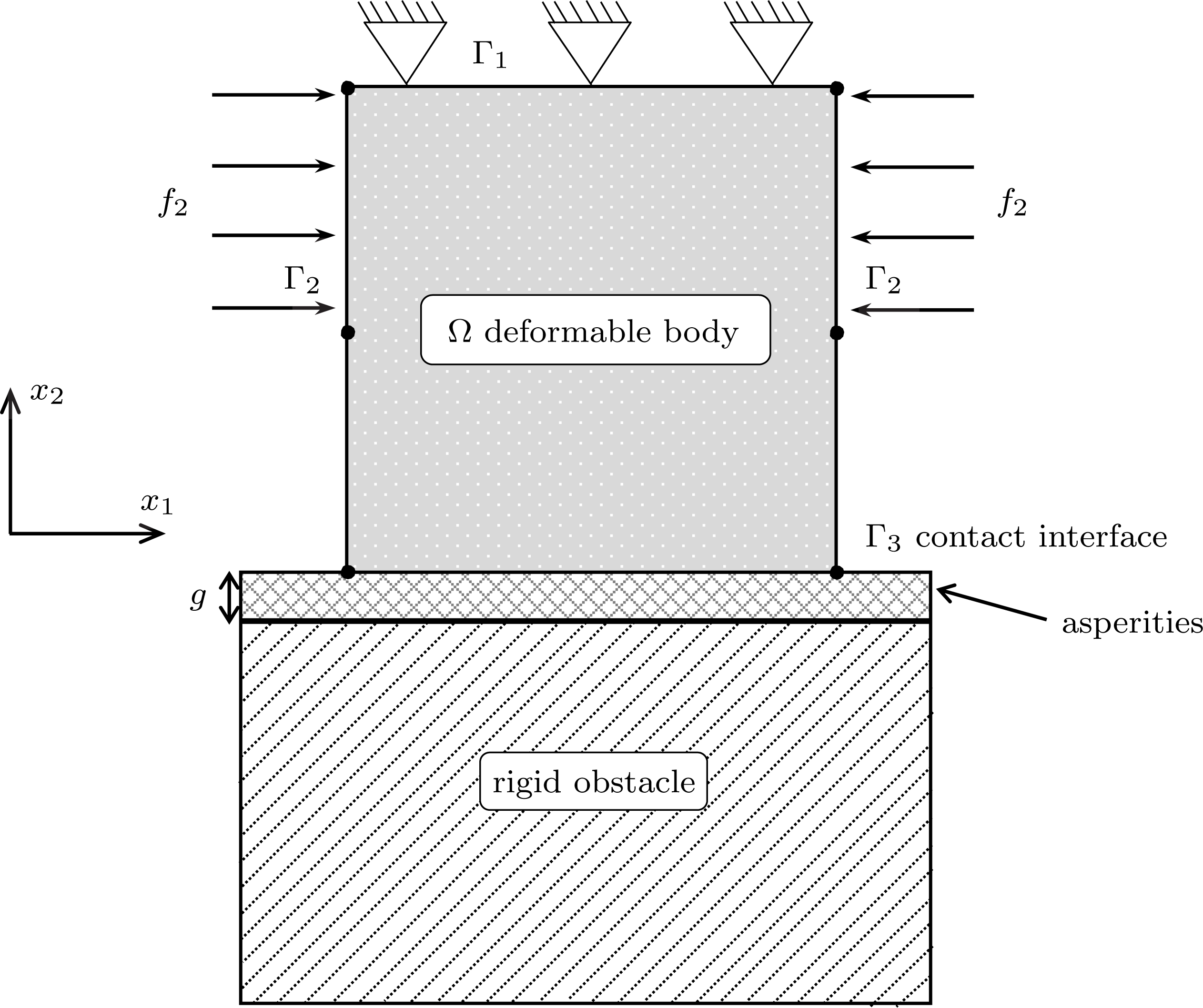
We now present numerical simulation results for the linear finite element solution of Problem 2.6 and its frictionless counterpart, i.e. the hemivariational inequality (7.30). The numerical results are adapted from Sofonea, Han and Barboteu (Reference Sofonea, Han, Barboteu and dell’Isola2017) and Han, Sofonea and Barboteu (Reference Han, Sofonea and Barboteu2017), respectively. For both numerical examples, we use the physical setting shown in Figure 7.1. The domain
 $\unicode[STIX]{x1D6FA}$
represents the cross-section of a three-dimensional linearly elastic body such that the plane stress hypothesis is valid. We take
 $\unicode[STIX]{x1D6FA}=(0,1)\times (0,1)\subset \mathbb{R}^{2}$
to be the unit square and partition the boundary as follows:
 $$\begin{eqnarray}\unicode[STIX]{x1D6E4}_{1}=[0,1]\times \{1\},\quad \unicode[STIX]{x1D6E4}_{2}=(\{0\}\times (0,1))\cup (\{1\}\times (0,1)),\quad \unicode[STIX]{x1D6E4}_{3}=[0,1]\times \{0\}.\end{eqnarray}$$
The body is clamped on
 $\unicode[STIX]{x1D6E4}_{1}$
, and is subject to the actions of a vertical body force of constant density and of horizontally compressive forces on the part
 $(\{0\}\times [0.5,1))\cup (\{1\}\times [0.5,1))$
of the boundary
 $\unicode[STIX]{x1D6E4}_{2}$
. The part
 $(\{0\}\times (0,0.5))\cup (\{1\}\times (0,0.5))$
is traction-free. The body is in contact with an obstacle on
 $\unicode[STIX]{x1D6E4}_{3}$
. For numerical simulations, linear finite elements on uniform triangulations of the domain
 $\unicode[STIX]{x1D6FA}$
are used. Each side of the boundary of the domain is divided into
 $1/h$
equal parts, and
 $h$
is used as the discretization parameter.
The mechanical response of the material is described by a linear elastic constitutive law. In terms of the components, the elasticity tensor
 ${\mathcal{F}}$
is defined by the relations
 $$\begin{eqnarray}({\mathcal{F}}\unicode[STIX]{x1D749})_{ij}=\displaystyle \frac{E\unicode[STIX]{x1D705}}{1-\unicode[STIX]{x1D705}^{2}}(\unicode[STIX]{x1D70F}_{11}+\unicode[STIX]{x1D70F}_{22})\unicode[STIX]{x1D6FF}_{ij}+\displaystyle \frac{E}{1+\unicode[STIX]{x1D705}}\unicode[STIX]{x1D70F}_{ij},\quad 1\leq i,j\leq 2,~\text{for all}~\unicode[STIX]{x1D749}\in \mathbb{S}^{2},\end{eqnarray}$$
where
 $E$
and
 $\unicode[STIX]{x1D705}$
are the Young’s modulus and Poisson ratio of the material,
 $\unicode[STIX]{x1D6FF}_{ij}$
is the Kronecker delta symbol. For both numerical examples, we use
 $$\begin{eqnarray}\displaystyle E & = & \displaystyle 2000~\text{N}~\text{m}^{-2},\quad \unicode[STIX]{x1D705}=0.4,\nonumber\\ \displaystyle \boldsymbol{f}_{0} & = & \displaystyle (0,-0.5\times 10^{-3})~\text{N}~\text{m}^{-2},\nonumber\\ \displaystyle \boldsymbol{f}_{2} & = & \displaystyle \left\{\begin{array}{@{}ll@{}}(8\times 10^{-3},0)~\text{N}~\text{m}^{-1}\quad & \text{on }\{0\}\times [0.5,1),\\ (-8\times 10^{-3},0)~\text{N}~\text{m}^{-1}\quad & \text{on }\{1\}\times [0.5,1).\end{array}\right.\nonumber\end{eqnarray}$$
Deformed meshes and interface forces on
 $\unicode[STIX]{x1D6E4}_{3}$
for the first example.
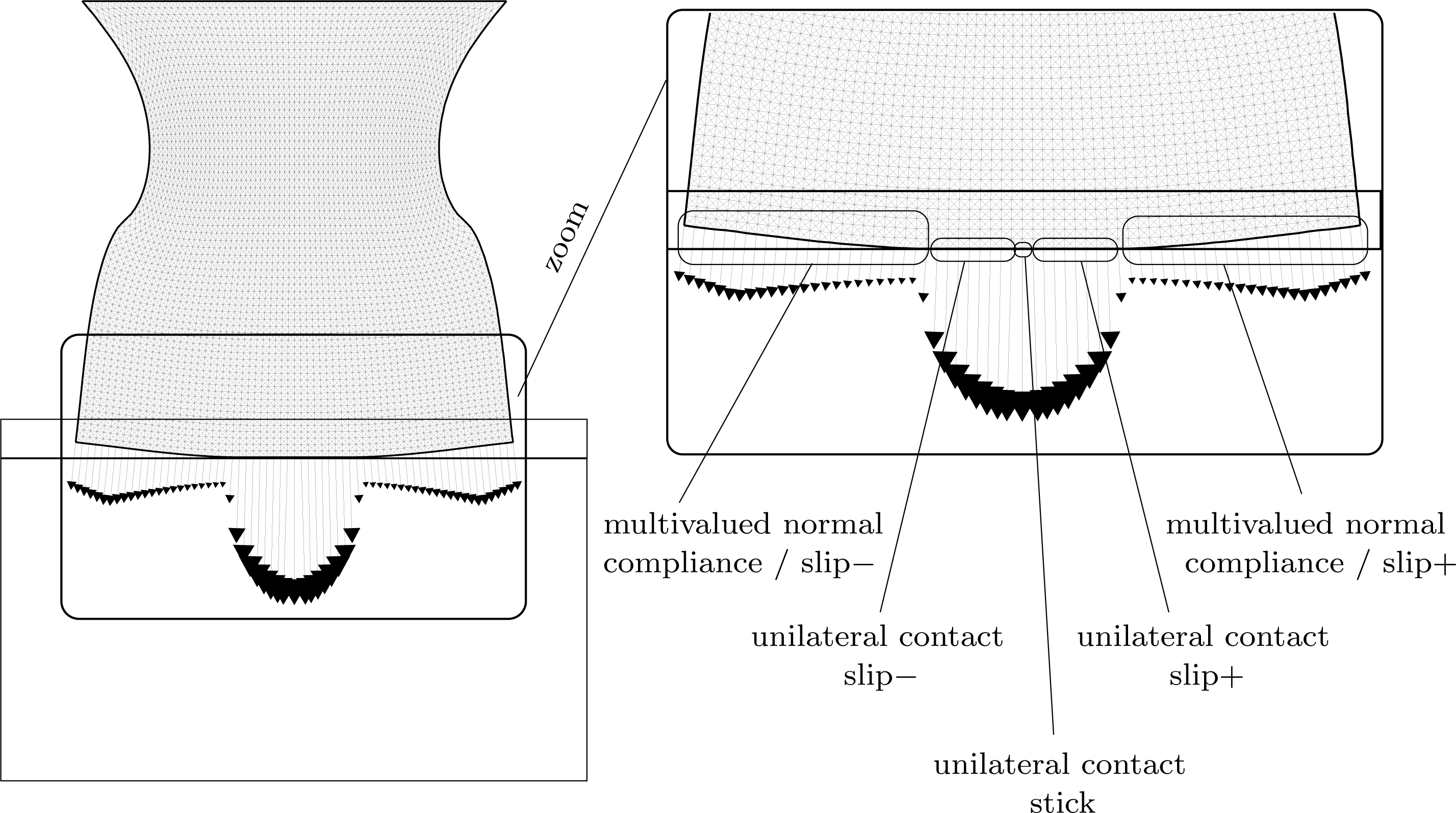
Relative errors in energy norm for the first example.
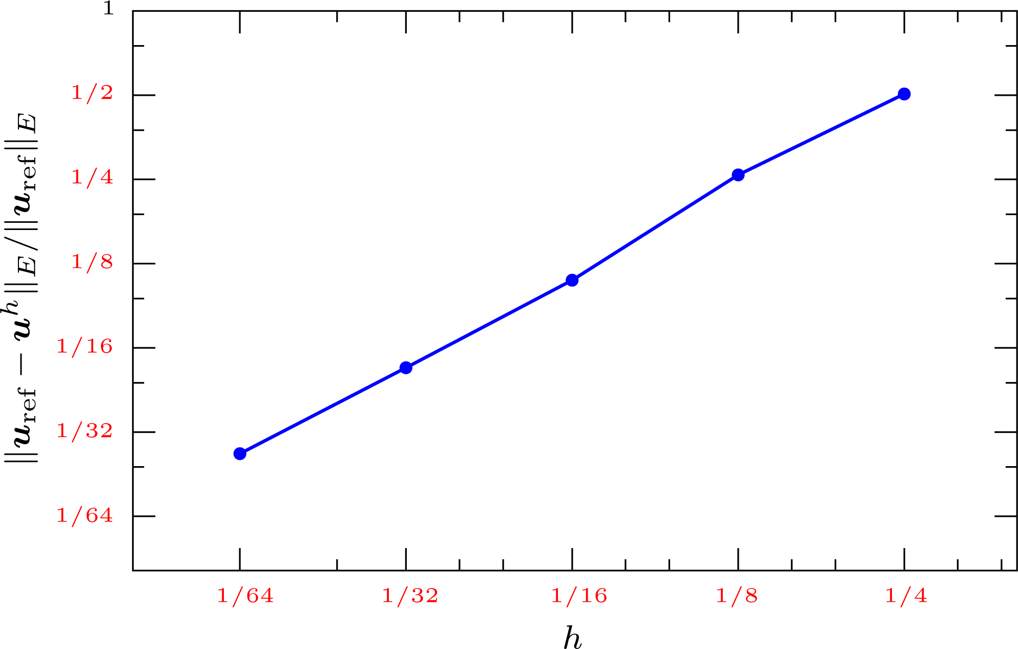
To describe the contact condition on the subset
 $\unicode[STIX]{x1D6E4}_{3}=[0,1]\times \{0\}$
of the boundary, we let
 $0<r_{\unicode[STIX]{x1D708}1}<r_{\unicode[STIX]{x1D708}2}$
be given, and define two functions
 $p_{\unicode[STIX]{x1D708}}:\mathbb{R}\rightarrow \mathbb{R}$
and
 $j_{\unicode[STIX]{x1D708}}:\mathbb{R}\rightarrow \mathbb{R}$
by
 $$\begin{eqnarray}p_{\unicode[STIX]{x1D708}}(r)=\left\{\begin{array}{@{}ll@{}}0\quad & \text{if}~r\leq 0,\\ c_{\unicode[STIX]{x1D708}1}r\quad & \text{if}~r\in (0,r_{\unicode[STIX]{x1D708}1}],\\ c_{\unicode[STIX]{x1D708}1}r_{\unicode[STIX]{x1D708}1}+c_{\unicode[STIX]{x1D708}2}(r-r_{\unicode[STIX]{x1D708}1})\quad & \text{if}~r\in (r_{\unicode[STIX]{x1D708}1},r_{\unicode[STIX]{x1D708}2}),\\ c_{\unicode[STIX]{x1D708}1}r_{\unicode[STIX]{x1D708}1}+c_{\unicode[STIX]{x1D708}2}(r_{\unicode[STIX]{x1D708}2}-r_{\unicode[STIX]{x1D708}1})+c_{\unicode[STIX]{x1D708}3}(r-r_{\unicode[STIX]{x1D708}2})\quad & \text{if}~r\geq r_{\unicode[STIX]{x1D708}2},\end{array}\right.\end{eqnarray}$$
and
 $$\begin{eqnarray}j_{\unicode[STIX]{x1D708}}(r)=\int _{0}^{r}p_{\unicode[STIX]{x1D708}}(s)\,\text{d}s,\quad r\in \mathbb{R},\end{eqnarray}$$
respectively. Here
 $c_{\unicode[STIX]{x1D708}1}>0$
,
 $c_{\unicode[STIX]{x1D708}2}<0$
and
 $c_{\unicode[STIX]{x1D708}3}>0$
are given constants. Then
 $$\begin{eqnarray}F_{b}(r)=\unicode[STIX]{x1D707}\,p_{\unicode[STIX]{x1D708}}(r),\quad r\in \mathbb{R},\end{eqnarray}$$
where
 $\unicode[STIX]{x1D707}\geq 0$
represents a given coefficient of friction. The function
 $p_{\unicode[STIX]{x1D708}}$
is continuous but not monotone, and therefore
 $j_{\unicode[STIX]{x1D708}}$
is a locally Lipschitz non-convex function. In both examples we take
 $c_{\unicode[STIX]{x1D708}1}=100~\text{N}~\text{m}^{-2}$
,
 $c_{\unicode[STIX]{x1D708}2}=-100~\text{N}~\text{m}^{-2}$
,
 $c_{\unicode[STIX]{x1D708}3}=400~\text{N}~\text{m}^{-2}$
,
 $r_{\unicode[STIX]{x1D708}1}=0.1$
m,
 $r_{\unicode[STIX]{x1D708}2}=0.15$
m and
 $g=0.15$
m. Note that
 $g$
represents the maximally allowed amount of penetration.
In the first numerical example, the frictional contact condition on
 $\unicode[STIX]{x1D6E4}_{3}$
takes the following form:
 $$\begin{eqnarray}\displaystyle & & \displaystyle u_{\unicode[STIX]{x1D708}}\leq g,\quad \unicode[STIX]{x1D70E}_{\unicode[STIX]{x1D708}}+\unicode[STIX]{x1D709}_{\unicode[STIX]{x1D708}}\leq 0,\quad (u_{\unicode[STIX]{x1D708}}-g)(\unicode[STIX]{x1D70E}_{\unicode[STIX]{x1D708}}+\unicode[STIX]{x1D709}_{\unicode[STIX]{x1D708}})=0,\end{eqnarray}$$
 $$\begin{eqnarray}\displaystyle & & \displaystyle \unicode[STIX]{x1D709}_{\unicode[STIX]{x1D708}}=p_{\unicode[STIX]{x1D708}}(u_{\unicode[STIX]{x1D708}}),\end{eqnarray}$$
 $$\begin{eqnarray}\displaystyle & & \displaystyle \Vert \unicode[STIX]{x1D748}_{\unicode[STIX]{x1D70F}}\Vert \leq \unicode[STIX]{x1D707}\,\unicode[STIX]{x1D709}_{\unicode[STIX]{x1D708}},\quad -\unicode[STIX]{x1D748}_{\unicode[STIX]{x1D70F}}=\unicode[STIX]{x1D707}\,\unicode[STIX]{x1D709}_{\unicode[STIX]{x1D708}}\,\displaystyle \frac{\boldsymbol{u}_{\unicode[STIX]{x1D70F}}}{\Vert \boldsymbol{u}_{\unicode[STIX]{x1D70F}}\Vert }\quad \text{if }~\boldsymbol{u}_{\unicode[STIX]{x1D70F}}\not =\mathbf{0}.\end{eqnarray}$$
The deformed mesh and the distribution of the interface forces on
 $\unicode[STIX]{x1D6E4}_{3}$
are reported in Figure 7.2 corresponding to a mesh-size
 $h=1/64$
. We observe that the contact boundary
 $\unicode[STIX]{x1D6E4}_{3}$
can be split into two parts depending on whether the penetration bound is reached. More precisely, for some number
 $\unicode[STIX]{x1D6FF}_{1}\in (0,1/2)$
,
 $\unicode[STIX]{x1D6E4}_{3}$
can be expressed as the union of three subsets
 $\unicode[STIX]{x1D6E4}_{3\,1}=[0,1/2-\unicode[STIX]{x1D6FF}_{1})\times \{0\}$
,
 $\unicode[STIX]{x1D6E4}_{3\,2}=[1/2-\unicode[STIX]{x1D6FF}_{1},1/2+\unicode[STIX]{x1D6FF}_{1}]\times \{0\}$
and
 $\unicode[STIX]{x1D6E4}_{3\,3}=(1/2+\unicode[STIX]{x1D6FF}_{1},1]\times \{0\}$
such that the contact nodes on
 $\unicode[STIX]{x1D6E4}_{3\,1}$
are in multivalued normal compliance status with backward slip (slip
 $-$
), those on
 $\unicode[STIX]{x1D6E4}_{3\,3}$
are in multivalued normal compliance status with forward slip (slip+), and the nodes on
 $\unicode[STIX]{x1D6E4}_{3\,2}$
are in unilateral contact. Note that on
 $\unicode[STIX]{x1D6E4}_{3\,1}\cup \unicode[STIX]{x1D6E4}_{3\,3}$
the normal displacement
 $u_{\unicode[STIX]{x1D708}}$
does not reach the penetration bound, i.e.
 $u_{\unicode[STIX]{x1D708}}<g$
, whereas on
 $\unicode[STIX]{x1D6E4}_{3\,2}$
the penetration bound is reached, i.e.
 $u_{\unicode[STIX]{x1D708}}=g$
. Most of the nodes on
 $\unicode[STIX]{x1D6E4}_{3\,2}$
are in slip status, except the node at the centre of
 $\unicode[STIX]{x1D6E4}_{3\,2}$
which is in stick status.
In Figure 7.3, we report relative errors of the numerical solutions in the energy norm,
 $\Vert \boldsymbol{u}_{\text{ref}}-\boldsymbol{u}^{h}\Vert _{E}/\Vert \boldsymbol{u}_{\text{ref}}\Vert _{E}$
, where the energy norm is defined by the formula
 $$\begin{eqnarray}\Vert \boldsymbol{v}\Vert _{E}:=\displaystyle \frac{1}{\sqrt{2}}({\mathcal{F}}(\unicode[STIX]{x1D73A}(\boldsymbol{v})),\unicode[STIX]{x1D73A}(\boldsymbol{v}))_{Q}^{1/2}.\end{eqnarray}$$
Note that the energy norm
 $\Vert \boldsymbol{v}\Vert _{E}$
is equivalent to the norm
 $\Vert \boldsymbol{v}\Vert _{V}$
, and the error bound (7.28) predicts an optimal first-order convergence of the numerical solutions measured in the energy norm, under the regularity assumptions (7.18) and (7.27), which take the form
 $$\begin{eqnarray}\boldsymbol{u}\in H^{2}(\unicode[STIX]{x1D6FA};\mathbb{R}^{2}),\quad \boldsymbol{u}|_{\unicode[STIX]{x1D6E4}_{3}}\in H^{2}(\unicode[STIX]{x1D6E4}_{3};\mathbb{R}^{2}).\end{eqnarray}$$
Since the true solution
 $\boldsymbol{u}$
is not available, we use the numerical solution corresponding to a fine discretization of
 $\unicode[STIX]{x1D6FA}$
as the ‘reference’ solution
 $\boldsymbol{u}_{\text{ref}}$
in computing the solution errors. Here, the numerical solution with
 $h=1/256$
is taken to be the ‘reference’ solution
 $\boldsymbol{u}_{\text{ref}}$
. We clearly observe the theoretically predicted optimal linear convergence of the numerical solutions.
In the second numerical example, the contact boundary conditions on
 $\unicode[STIX]{x1D6E4}_{3}$
are characterized by a frictionless multivalued normal compliance contact in which the penetration is restricted by the unilateral constraint. For simulations, on
 $\unicode[STIX]{x1D6E4}_{3}$
, we use (7.35), (7.36), and replace (7.37) with
 $$\begin{eqnarray}\unicode[STIX]{x1D748}_{\unicode[STIX]{x1D70F}}=\mathbf{0}.\end{eqnarray}$$
It follows from Han, Sofonea and Barboteu (Reference Han, Sofonea and Barboteu2017) that for the linear element solution of the corresponding hemivariational inequality we again have the optimal order error bound (7.28) under the regularity assumptions (7.38).
The numerical results on the deformed mesh and the distribution of the interface forces on
 $\unicode[STIX]{x1D6E4}_{3}$
are shown in Figure 7.4 for a mesh-size
 $h=1/64$
. As in the first example, the contact boundary
 $\unicode[STIX]{x1D6E4}_{3}$
can be split into three subsets
 $\unicode[STIX]{x1D6E4}_{3\,1}=[0,1/2-\unicode[STIX]{x1D6FF}_{2})\times \{0\}$
,
 $\unicode[STIX]{x1D6E4}_{3\,2}=[1/2-\unicode[STIX]{x1D6FF}_{2},1/2+\unicode[STIX]{x1D6FF}_{2}]\times \{0\}$
and
 $\unicode[STIX]{x1D6E4}_{3\,3}=(1/2+\unicode[STIX]{x1D6FF}_{2},1]\times \{0\}$
, for some number
 $\unicode[STIX]{x1D6FF}_{2}\in (0,1/2)$
, such that the nodes on
 $\unicode[STIX]{x1D6E4}_{3\,1}\cup \unicode[STIX]{x1D6E4}_{3\,3}$
are in multivalued normal compliance status, whereas the nodes on
 $\unicode[STIX]{x1D6E4}_{3\,2}$
are in unilateral contact status where the penetration reaches the upper bound
 $g$
.
Deformed meshes and interface forces on
 $\unicode[STIX]{x1D6E4}_{3}$
for the second example.
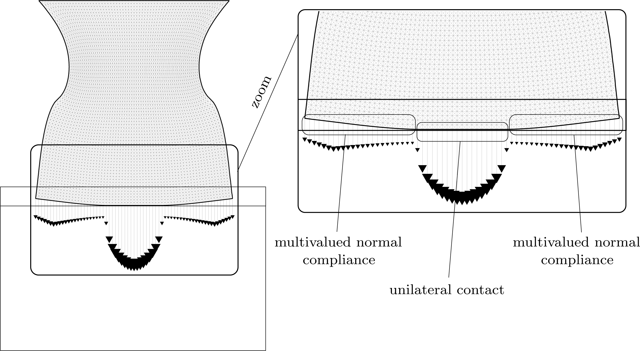
Relative errors in energy norm for the second example.
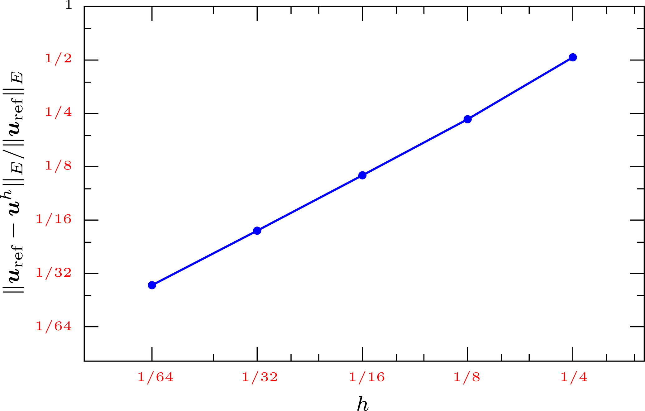
In Figure 7.5 we report relative errors of the numerical solutions in the energy norm,
 $\Vert \boldsymbol{u}_{\text{ref}}-\boldsymbol{u}^{h}\Vert _{E}/\Vert \boldsymbol{u}_{\text{ref}}\Vert _{E}$
. Again, we use the numerical solution corresponding to
 $h=1/256$
as the ‘reference’ solution
 $\boldsymbol{u}_{\text{ref}}$
in computing the solution errors. Once more, we clearly observe the theoretically predicted optimal linear convergence of the numerical solutions.
8 Studies of the history-dependent contact problem
In this section we study the history-dependent contact problem, Problem 2.8. We first explore the solution existence and uniqueness, then introduce a linear finite element method and derive an optimal order error estimate and, finally, present numerical simulation results.
8.1 Solution existence and uniqueness
Recall that
 $\unicode[STIX]{x1D706}_{1\unicode[STIX]{x1D708}}>0$
is the smallest eigenvalue of the eigenvalue problem (7.4). The unique solvability of Problem 2.8 is given by the following existence and uniqueness result.
Theorem 8.1. Assume (2.34), (2.35), (2.38), (2.51), (2.52) and
 $$\begin{eqnarray}\unicode[STIX]{x1D6FC}_{j_{\unicode[STIX]{x1D708}}}\unicode[STIX]{x1D706}_{1\unicode[STIX]{x1D708}}^{-1}<m_{{\mathcal{F}}}.\end{eqnarray}$$
Then Problem 2.8 has a unique solution
 $\boldsymbol{u}\in C(I;U)$
.
Proof. Let
 $X=V$
as defined in (2.3),
 $Y=Q$
as defined in (2.4),
 $K=U$
as defined in (2.39),
 $X_{j}=V_{j}$
as defined in (7.2), and let
 $\unicode[STIX]{x1D6FE}_{j}:V\rightarrow V_{j}$
be the normal trace operator. We introduce operators and functionals
 $A:V\rightarrow V^{\ast }$
,
 ${\mathcal{S}}:C(I;V)\rightarrow C(I;Q)$
,
 $\unicode[STIX]{x1D711}:Q\times V\times V\rightarrow \mathbb{R}$
,
 $j:V_{j}\rightarrow \mathbb{R}$
and
 $\boldsymbol{f}:I\rightarrow V^{\ast }$
as follows:
 $$\begin{eqnarray}\displaystyle \langle A\boldsymbol{u},\boldsymbol{v}\rangle & = & \displaystyle \int _{\unicode[STIX]{x1D6FA}}{\mathcal{F}}\unicode[STIX]{x1D73A}(\boldsymbol{u})\cdot \unicode[STIX]{x1D73A}(\boldsymbol{v})\,\text{d}x,\quad \boldsymbol{u},\boldsymbol{v}\in V,\end{eqnarray}$$
 $$\begin{eqnarray}\displaystyle {\mathcal{S}}\boldsymbol{u}(t) & = & \displaystyle \int _{0}^{t}{\mathcal{B}}(t-s)\unicode[STIX]{x1D73A}(\boldsymbol{u}(s))\,\text{d}s,\quad \boldsymbol{u}\in C(I;V),\end{eqnarray}$$
 $$\begin{eqnarray}\displaystyle \unicode[STIX]{x1D711}(\boldsymbol{y},\boldsymbol{u},\boldsymbol{v}) & = & \displaystyle \int _{\unicode[STIX]{x1D6FA}}\boldsymbol{y}\cdot \unicode[STIX]{x1D73A}(\boldsymbol{v})\,\text{d}x,\quad \boldsymbol{y}\in Q,\,\boldsymbol{u},\boldsymbol{v}\in V,\end{eqnarray}$$
 $$\begin{eqnarray}\displaystyle j(z) & = & \displaystyle \int _{\unicode[STIX]{x1D6E4}_{3}}j_{\unicode[STIX]{x1D708}}(z)\,\text{d}a,\quad z\in V_{j},\end{eqnarray}$$
 $$\begin{eqnarray}\displaystyle \langle \boldsymbol{f}(t),\boldsymbol{v}\rangle & = & \displaystyle \int _{\unicode[STIX]{x1D6FA}}\boldsymbol{f}_{0}(t)\cdot \boldsymbol{v}\,\text{d}x+\int _{\unicode[STIX]{x1D6E4}_{2}}\boldsymbol{f}_{2}(t)\cdot \boldsymbol{v}\,\text{d}a,\quad \boldsymbol{v}\in V.\end{eqnarray}$$
Consider the problem of finding a function
 $\boldsymbol{u}:I\rightarrow U$
such that for each
 $t\in I$
, the following inequality holds:
 $$\begin{eqnarray}\displaystyle & & \displaystyle \langle A\boldsymbol{u}(t),\boldsymbol{v}-\boldsymbol{u}(t)\rangle +\unicode[STIX]{x1D711}({\mathcal{S}}\boldsymbol{u}(t),\boldsymbol{u}(t),\boldsymbol{v})-\unicode[STIX]{x1D711}({\mathcal{S}}\boldsymbol{u}(t),\boldsymbol{u}(t),\boldsymbol{u}(t))\nonumber\\ \displaystyle & & \displaystyle \quad +j^{0}(\unicode[STIX]{x1D6FE}_{j}\boldsymbol{u}(t);\unicode[STIX]{x1D6FE}_{j}\boldsymbol{v}-\unicode[STIX]{x1D6FE}_{j}\boldsymbol{u}(t))\geq \langle \boldsymbol{f}(t),\boldsymbol{v}-\boldsymbol{u}(t)\rangle \quad \text{for all}~\boldsymbol{v}\in U.\end{eqnarray}$$
We can apply Theorem 5.4 to see that inequality (8.7) has a unique solution
 $\boldsymbol{u}\in C(I;U)$
. The argument is similar to that used in the proof of Theorem 7.1, so we only give a sketch of the proof. Note that the function
 $\unicode[STIX]{x1D711}$
defined by (8.4) satisfies condition (5.3) with
 $\unicode[STIX]{x1D6FC}_{\unicode[STIX]{x1D711}}=0$
and
 $\unicode[STIX]{x1D6FD}_{\unicode[STIX]{x1D711}}=1$
. From assumption (2.51) and inequality (2.9) we deduce that the operator
 ${\mathcal{S}}:C(I;V)\rightarrow C(I;Q)$
defined by (8.3) is a history-dependent operator. The smallness condition (5.11) follows from (8.1). Use inequality (7.11) to see that
 $\boldsymbol{u}$
is a solution to Problem 2.8. This proves the existence part of Theorem 8.1. The uniqueness part follows from a standard argument, similar to that in the last part of the proof of Theorem 7.1, combined with the Gronwall argument. ◻
8.2 Numerical analysis of the problem
Throughout this subsection, we keep the assumptions stated in Theorem 8.1 so that we are assured that Problem 2.8 has a unique solution
 $\boldsymbol{u}\in C(I;U)$
. We now proceed with the discretization of Problem 2.8. We use the finite element space
 $V^{h}$
and the finite element set
 $U^{h}$
as in Section 7.2. Here and below for any vector field
 $\boldsymbol{z}_{i}$
we use the notation
 $z_{i,\unicode[STIX]{x1D708}}$
and
 $\boldsymbol{z}_{i,\unicode[STIX]{x1D70F}}$
to represent its normal and tangential components, respectively.
Assume
 $g$
is a continuous concave function. Then,
 $U^{h}\subset U$
. Thus the approximation is internal and the numerical method for Problem 2.8 is defined as follows.
Problem 8.2. Find a discrete displacement
 $\boldsymbol{u}^{hk}:=\{\boldsymbol{u}_{n}^{hk_{}^{}\}}\subset U^{h}$
such that for
 $0\leq n\leq N$
and for all
 $\boldsymbol{v}^{h}\in U^{h}$
,
 $$\begin{eqnarray}\displaystyle & & \displaystyle \int _{\unicode[STIX]{x1D6FA}}{\mathcal{F}}\unicode[STIX]{x1D73A}(\boldsymbol{u}_{n}^{hk})\cdot (\unicode[STIX]{x1D73A}(\boldsymbol{v}^{h})-\unicode[STIX]{x1D73A}(\boldsymbol{u}_{n}^{hk}))\,\text{d}x+\int _{\unicode[STIX]{x1D6FA}}{\mathcal{S}}_{n}^{k}\boldsymbol{u}^{hk}\cdot (\unicode[STIX]{x1D73A}(\boldsymbol{v}^{h})-\unicode[STIX]{x1D73A}(\boldsymbol{u}_{n}^{hk}))\,\text{d}x\nonumber\\ \displaystyle & & \displaystyle \quad +\int _{\unicode[STIX]{x1D6E4}_{3}}j_{\unicode[STIX]{x1D708}}^{0}(u_{n,\unicode[STIX]{x1D708}}^{hk};v_{\unicode[STIX]{x1D708}}^{h}-u_{n,\unicode[STIX]{x1D708}}^{hk})\,\text{d}a\nonumber\\ \displaystyle & & \displaystyle \quad \quad \geq \int _{\unicode[STIX]{x1D6FA}}\boldsymbol{f}_{0}(t_{n})\cdot (\boldsymbol{v}^{h}-\boldsymbol{u}_{n}^{hk})\,\text{d}x+\int _{\unicode[STIX]{x1D6E4}_{2}}\boldsymbol{f}_{2}(t_{n})\cdot (\boldsymbol{v}^{h}-\boldsymbol{u}_{n}^{hk})\,\text{d}a,\end{eqnarray}$$
where
 $$\begin{eqnarray}{\mathcal{S}}_{n}^{k}\boldsymbol{u}^{hk}=k\mathop{\sum }_{i=0}^{n}\hspace{-1.0pt}\text{}^{\prime }{\mathcal{B}}(t_{n}-t_{i})\,\unicode[STIX]{x1D73A}(\boldsymbol{u}_{i}^{hk}).\end{eqnarray}$$
It is straightforward to check that the derivation of the error inequality (5.35) in Theorem 5.10 is valid when the term
 $j^{0}(\unicode[STIX]{x1D6FE}_{j}u_{n}^{hk};\unicode[STIX]{x1D6FE}_{j}v^{h}-\unicode[STIX]{x1D6FE}_{j}u_{n}^{hk})$
in (5.34) is replaced by
 $\int _{\unicode[STIX]{x1D6E4}_{3}}j_{\unicode[STIX]{x1D708}}^{0}(u_{n,\unicode[STIX]{x1D708}}^{hk};v_{\unicode[STIX]{x1D708}}^{h}-u_{n,\unicode[STIX]{x1D708}}^{hk})\,\text{d}a$
as in (8.8). Recall that, here and below,
 $u_{n,\unicode[STIX]{x1D708}}^{hk}$
denotes the normal component of the vector field
 $\boldsymbol{u}_{n}^{hk}$
.
To derive an error estimate for the numerical solution defined by Problem 8.2, we need to bound the residual term defined in (5.36):
 $$\begin{eqnarray}\displaystyle R_{n}(\boldsymbol{v}^{h},\boldsymbol{u}_{n}) & = & \displaystyle \langle A\boldsymbol{u}_{n},\boldsymbol{v}^{h}-\boldsymbol{u}_{n}\rangle +\unicode[STIX]{x1D711}({\mathcal{S}}_{n}\boldsymbol{u},\boldsymbol{u}_{n},\boldsymbol{v}^{h})-\unicode[STIX]{x1D711}({\mathcal{S}}_{n}\boldsymbol{u},\boldsymbol{u}_{n},\boldsymbol{u}_{n})\nonumber\\ \displaystyle & & \displaystyle +\,\int _{\unicode[STIX]{x1D6E4}_{3}}j_{\unicode[STIX]{x1D708}}^{0}(u_{n,\unicode[STIX]{x1D708}};v_{\unicode[STIX]{x1D708}}^{h}-u_{n,\unicode[STIX]{x1D708}})\,\text{d}a-\langle \mathbf{f}_{n},\mathbf{v}^{h}-\mathbf{u}_{n}\rangle .\end{eqnarray}$$
For this purpose, we assume the following solution regularity property:
 $$\begin{eqnarray}\boldsymbol{u}\in W^{2,\infty }(I;V).\end{eqnarray}$$
For all
 $t\in I$
define
 $$\begin{eqnarray}\unicode[STIX]{x1D748}(t)={\mathcal{F}}\unicode[STIX]{x1D73A}(\boldsymbol{u}(t))+\int _{0}^{t}{\mathcal{B}}(t-s)\,\unicode[STIX]{x1D73A}(\boldsymbol{u}(s))\,\text{d}s\quad \text{in}~\unicode[STIX]{x1D6FA}.\end{eqnarray}$$
Then
 $$\begin{eqnarray}\unicode[STIX]{x1D748}\in C(I;H^{1}(\unicode[STIX]{x1D6FA};\mathbb{S}^{d})),\quad \unicode[STIX]{x1D748}\unicode[STIX]{x1D742}\in C(I;L^{2}(\unicode[STIX]{x1D6E4};\mathbb{R}^{d})).\end{eqnarray}$$
We now derive some pointwise relations for the weak solution
 $\boldsymbol{u}$
, similar to what is done in Section 7.2. Define a subset of
 $U$
:
 $$\begin{eqnarray}\widetilde{U}=\{\boldsymbol{v}\in C^{\infty }(\overline{\unicode[STIX]{x1D6FA}})^{d}\mid \boldsymbol{v}=\mathbf{0}\text{ on }\unicode[STIX]{x1D6E4}_{1},\,v_{\unicode[STIX]{x1D708}}=0\text{ on }\unicode[STIX]{x1D6E4}_{3}\}.\end{eqnarray}$$
We take
 $\boldsymbol{v}=\boldsymbol{u}(t)\pm \widetilde{\boldsymbol{v}}$
in (2.53), where
 $\widetilde{\boldsymbol{v}}\in \widetilde{U}$
is arbitrary; this leads to
 $$\begin{eqnarray}(\unicode[STIX]{x1D748}(t),\unicode[STIX]{x1D73A}(\widetilde{\boldsymbol{v}}))_{L^{2}(\unicode[STIX]{x1D6FA};\mathbb{S}^{d})}=\langle \boldsymbol{f}(t),\widetilde{\boldsymbol{v}}\rangle _{V^{\ast }\times V}\quad \text{for all}~\widetilde{\boldsymbol{v}}\in \widetilde{U}.\end{eqnarray}$$
From this identity, we can deduce that
 $$\begin{eqnarray}\displaystyle & & \displaystyle \text{Div}\,\unicode[STIX]{x1D748}(t)+\boldsymbol{f}_{0}(t)=\mathbf{0}\quad \text{a.e. in }\unicode[STIX]{x1D6FA},\end{eqnarray}$$
 $$\begin{eqnarray}\displaystyle & & \displaystyle \unicode[STIX]{x1D748}(t)\unicode[STIX]{x1D742}=\boldsymbol{f}_{2}(t)\quad \text{a.e. on }\unicode[STIX]{x1D6E4}_{2},\quad \unicode[STIX]{x1D748}_{\unicode[STIX]{x1D70F}}(t)=\mathbf{0}\quad \text{a.e. on }\unicode[STIX]{x1D6E4}_{3}.\end{eqnarray}$$
Next, we multiply (8.12) by
 $\boldsymbol{v}-\boldsymbol{u}(t)$
with
 $\boldsymbol{v}\in U$
, integrate over
 $\unicode[STIX]{x1D6FA}$
, and perform an integration by parts:
 $$\begin{eqnarray}\displaystyle & & \displaystyle -\int _{\unicode[STIX]{x1D6FA}}\unicode[STIX]{x1D748}(t)\cdot (\unicode[STIX]{x1D73A}(\boldsymbol{v})-\unicode[STIX]{x1D73A}(\boldsymbol{u}(t)))\,\text{d}x\nonumber\\ \displaystyle & & \displaystyle \quad +\int _{\unicode[STIX]{x1D6E4}}\unicode[STIX]{x1D748}(t)\unicode[STIX]{x1D742}\cdot (\boldsymbol{v}-\boldsymbol{u}(t))\,\text{d}a+\int _{\unicode[STIX]{x1D6FA}}\mathbf{f_{0}}\cdot (\boldsymbol{v}-\boldsymbol{u}(t))\,\text{d}x=0.\nonumber\end{eqnarray}$$
Thus, at any
 $t\in I$
, for any
 $\boldsymbol{v}\in U$
, we have
 $$\begin{eqnarray}\int _{\unicode[STIX]{x1D6FA}}\unicode[STIX]{x1D748}(t)\cdot (\unicode[STIX]{x1D73A}(\boldsymbol{v})-\unicode[STIX]{x1D73A}(\boldsymbol{u}(t)))\,\text{d}x=\langle \boldsymbol{f}(t),\boldsymbol{v}-\boldsymbol{u}(t)\rangle _{V^{\ast }\times V}+\int _{\unicode[STIX]{x1D6E4}_{3}}\unicode[STIX]{x1D70E}_{\unicode[STIX]{x1D708}}(t)(v_{\unicode[STIX]{x1D708}}-u_{\unicode[STIX]{x1D708}}(t))\,\text{d}a.\end{eqnarray}$$
Take
 $\boldsymbol{v}=\boldsymbol{v}^{h}\in U^{h}$
in (8.14) at
 $t=t_{n}$
,
 $$\begin{eqnarray}\int _{\unicode[STIX]{x1D6FA}}\unicode[STIX]{x1D748}_{n}\cdot (\unicode[STIX]{x1D73A}(\boldsymbol{v}^{h})-\unicode[STIX]{x1D73A}(\boldsymbol{u}_{n}))\,\text{d}x=\langle \mathbf{f}_{n},\mathbf{v}^{h}-\mathbf{u}_{n}\rangle _{V^{\ast }\times V}+\int _{\unicode[STIX]{x1D6E4}_{3}}\unicode[STIX]{x1D70E}_{n,\unicode[STIX]{x1D708}}(v_{n,\unicode[STIX]{x1D708}}^{h}-u_{n,\unicode[STIX]{x1D708}})\,\text{d}a,\end{eqnarray}$$
which can be rewritten as
 $$\begin{eqnarray}\displaystyle & & \displaystyle \langle A\boldsymbol{u}_{n},\boldsymbol{v}^{h}-\boldsymbol{u}_{n}\rangle +\unicode[STIX]{x1D711}({\mathcal{S}}_{n}\boldsymbol{u},\boldsymbol{u}_{n},\boldsymbol{v}^{h})-\unicode[STIX]{x1D711}({\mathcal{S}}_{n}\boldsymbol{u},\boldsymbol{u}_{n},\boldsymbol{u}_{n})\nonumber\\ \displaystyle & & \displaystyle \quad =\langle \boldsymbol{f}_{n},\boldsymbol{v}^{h}-\boldsymbol{u}_{n}\rangle +\int _{\unicode[STIX]{x1D6E4}_{3}}\unicode[STIX]{x1D70E}_{n,\unicode[STIX]{x1D708}}(v_{\unicode[STIX]{x1D708}}^{h}-u_{n,\unicode[STIX]{x1D708}})\,\text{d}a.\end{eqnarray}$$
Thus, for the residual term of (8.9), we have
 $$\begin{eqnarray}R_{n}(\boldsymbol{v}^{h},\boldsymbol{u}_{n})=\int _{\unicode[STIX]{x1D6E4}_{3}}[\unicode[STIX]{x1D70E}_{n,\unicode[STIX]{x1D708}}(v_{\unicode[STIX]{x1D708}}^{h}-u_{n,\unicode[STIX]{x1D708}})+j_{\unicode[STIX]{x1D708}}^{0}(u_{n,\unicode[STIX]{x1D708}};v_{\unicode[STIX]{x1D708}}^{h}-u_{n,\unicode[STIX]{x1D708}})]\,\text{d}a.\end{eqnarray}$$
Using the solution regularity assumptions (8.10) and (8.11), we have
 $$\begin{eqnarray}|R_{n}(\boldsymbol{v}^{h},\boldsymbol{u}_{n})|\leq c\,\Vert u_{n,\unicode[STIX]{x1D708}}-v_{\unicode[STIX]{x1D708}}^{h}\Vert _{L^{2}(\unicode[STIX]{x1D6E4}_{3})}.\end{eqnarray}$$
Applying (5.35), we get
 $$\begin{eqnarray}\displaystyle & & \displaystyle \max _{0\leq n\leq N}\Vert \boldsymbol{u}_{n}-\boldsymbol{u}_{n}^{hk}\Vert _{V}\nonumber\\ \displaystyle & & \displaystyle \quad \leq c\max _{0\leq n\leq N}\inf _{\mathbf{v}^{h}\in V^{h}}[\Vert \boldsymbol{u}_{n}-\boldsymbol{v}^{h}\Vert _{V}+\Vert u_{n,\unicode[STIX]{x1D708}}-v_{\unicode[STIX]{x1D708}}^{h}\Vert _{L^{2}(\unicode[STIX]{x1D6E4}_{3})}^{1/2}]+c\,k^{2}.\end{eqnarray}$$
Recall that
 $$\begin{eqnarray}\overline{\unicode[STIX]{x1D6E4}_{3}}=\mathop{\bigcup }_{1\leq i\leq i_{3}}\unicode[STIX]{x1D6E4}_{3,i},\end{eqnarray}$$
where
 $\unicode[STIX]{x1D6E4}_{3,i}$
(
 $1\leq i\leq i_{3}$
) is a closed subset of an affine hyperplane. We further assume
 $$\begin{eqnarray}\boldsymbol{u}\in C(I;H^{2}(\unicode[STIX]{x1D6FA};\mathbb{R}^{d})),\quad u_{\unicode[STIX]{x1D708}}|_{\unicode[STIX]{x1D6E4}_{3,i}}\in C(I;H^{2}(\unicode[STIX]{x1D6E4}_{3,i})),~1\leq i\leq i_{3}.\end{eqnarray}$$
Then applying the finite element interpolation theory (e.g. Ciarlet Reference Ciarlet1978, Brenner and Scott Reference Brenner and Scott2008), we can derive the optimal order error bound
 $$\begin{eqnarray}\max _{0\leq n\leq N}\Vert \boldsymbol{u}_{n}-\boldsymbol{u}_{n}^{hk}\Vert _{V}\leq c(h+k^{2}).\end{eqnarray}$$
Hence, the method is first-order with respect to the spatial mesh-size and second-order with respect to the temporal step-size.
8.3 A numerical example
Here, we report a numerical example for Problem 2.8. The physical setting of the example is shown in Figure 8.1. The domain
 $\unicode[STIX]{x1D6FA}$
represents the cross-section of a three-dimensional linearly viscoelastic body such that the plane stress hypothesis is valid. For the numerical example, we take
 $\unicode[STIX]{x1D6FA}=(0,2)\times (0,1)$
with the metre as the length unit. The boundary
 $\unicode[STIX]{x1D6E4}=\unicode[STIX]{x2202}\unicode[STIX]{x1D6FA}$
is decomposed into three parts:
 $\unicode[STIX]{x1D6E4}_{1}$
where the body is fixed,
 $\unicode[STIX]{x1D6E4}_{2}$
where the body is subject to the action of surface traction, and
 $\unicode[STIX]{x1D6E4}_{3}$
where contact takes place. We take
 $\unicode[STIX]{x1D6E4}_{1}=\{0\}\times [0,1]$
,
 $\unicode[STIX]{x1D6E4}_{2}=\unicode[STIX]{x1D6E4}_{2\,1}\cup \unicode[STIX]{x1D6E4}_{2\,2}$
with
 $\unicode[STIX]{x1D6E4}_{2\,1}=\{2\}\times (0,1)$
and
 $\unicode[STIX]{x1D6E4}_{2\,2}=(0,2)\times \{1\}$
, and
 $\unicode[STIX]{x1D6E4}_{3}=[0,2]\times \{0\}$
.
Reference configuration of the two-dimensional body.
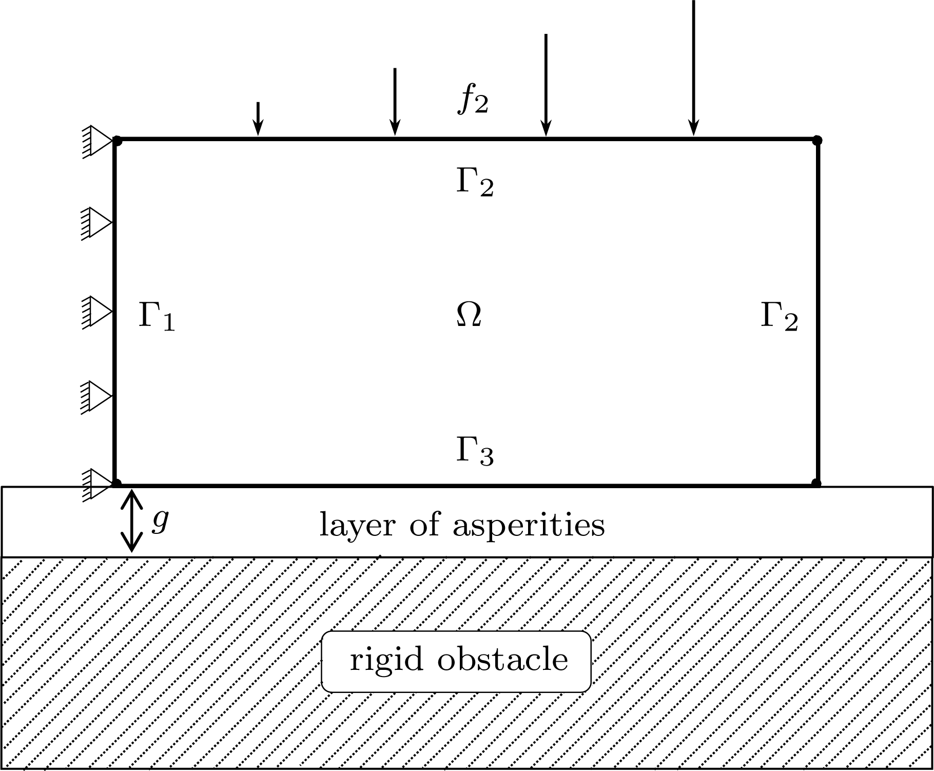
The elasticity tensor
 ${\mathcal{F}}$
is determined by the relations
 $$\begin{eqnarray}\displaystyle ({\mathcal{F}}\unicode[STIX]{x1D70F})_{ij}=\displaystyle \frac{E\unicode[STIX]{x1D705}}{1-\unicode[STIX]{x1D705}^{2}}(\unicode[STIX]{x1D70F}_{11}+\unicode[STIX]{x1D70F}_{22})\unicode[STIX]{x1D6FF}_{ij}+\displaystyle \frac{E}{1+\unicode[STIX]{x1D705}}\,\unicode[STIX]{x1D70F}_{ij},\quad 1\leq i,j\leq 2, & & \displaystyle\end{eqnarray}$$
where
 $E$
and
 $\unicode[STIX]{x1D705}$
are the Young’s modulus and Poisson ratio of the material, and
 $\unicode[STIX]{x1D6FF}_{ij}$
denotes the Kronecker delta symbol. In the numerical simulation, we choose
 $E=1~\text{N}~\text{m}^{-2}$
and
 $\unicode[STIX]{x1D705}=0.3$
.
The relaxation tensor is given by
 ${\mathcal{B}}(s)=(0.5+s)^{3}{\mathcal{I}}$
, where
 ${\mathcal{I}}$
denotes the identity tensor. For a given value
 $S\geq 0$
, the function
 $j_{\unicode[STIX]{x1D708}}(\cdot )$
is defined by
 $$\begin{eqnarray}j_{\unicode[STIX]{x1D708}}(u_{\unicode[STIX]{x1D708}})=S\int _{0}^{|u_{\unicode[STIX]{x1D708}}|}\unicode[STIX]{x1D707}(s)\,\text{d}s\end{eqnarray}$$
with
 $$\begin{eqnarray}\unicode[STIX]{x1D707}(s)=(a-b)\,\text{e}^{-\unicode[STIX]{x1D6FC}s}+b\end{eqnarray}$$
with
 $a\geq b>0$
and
 $\unicode[STIX]{x1D6FC}>0$
. We choose
 $S=0.1\,\text{N}$
,
 $\unicode[STIX]{x1D6FC}=100$
,
 $a=0.04$
,
 $b=0.02$
. The body force is ignored, and for the surface traction
 $$\begin{eqnarray}\displaystyle \boldsymbol{f}_{2}(\boldsymbol{x})=\left\{\begin{array}{@{}ll@{}}(0,0)~\text{N}~\text{m}^{-1}\quad & \text{on }\unicode[STIX]{x1D6E4}_{2\,1},\\ (0,-0.1(1-\text{e}^{-2t})x_{1})~\text{N}~\text{m}^{-1}\quad & \text{on }\unicode[STIX]{x1D6E4}_{2\,2}.\end{array}\right. & & \displaystyle \nonumber\end{eqnarray}$$
For the thickness function, we let
 $g=0.2$
m.
For the numerical solution of the problem, we introduce a family of rectangular finite element partitions as follows: given a positive integer
 $M$
, we divide the horizontal interval
 $[0,2]$
and the vertical interval
 $[0,1]$
into
 $M$
equal parts, and form the corresponding rectangular mesh with
 $M^{2}$
rectangular elements. We then construct the bilinear element space
 $V^{h}$
, with the finite element mesh parameter
 $h=1/M$
. Note that with the bilinear element replacing the linear element, the theoretical error estimate (8.20) stays the same.
Numerical evidence of first-order convergence of
 $\Vert \boldsymbol{u}_{\text{ref}}(\cdot ,1)-\boldsymbol{u}_{N}^{hk}\Vert _{1}$
(
 $N=1/k$
) with respect to
 $h$
.
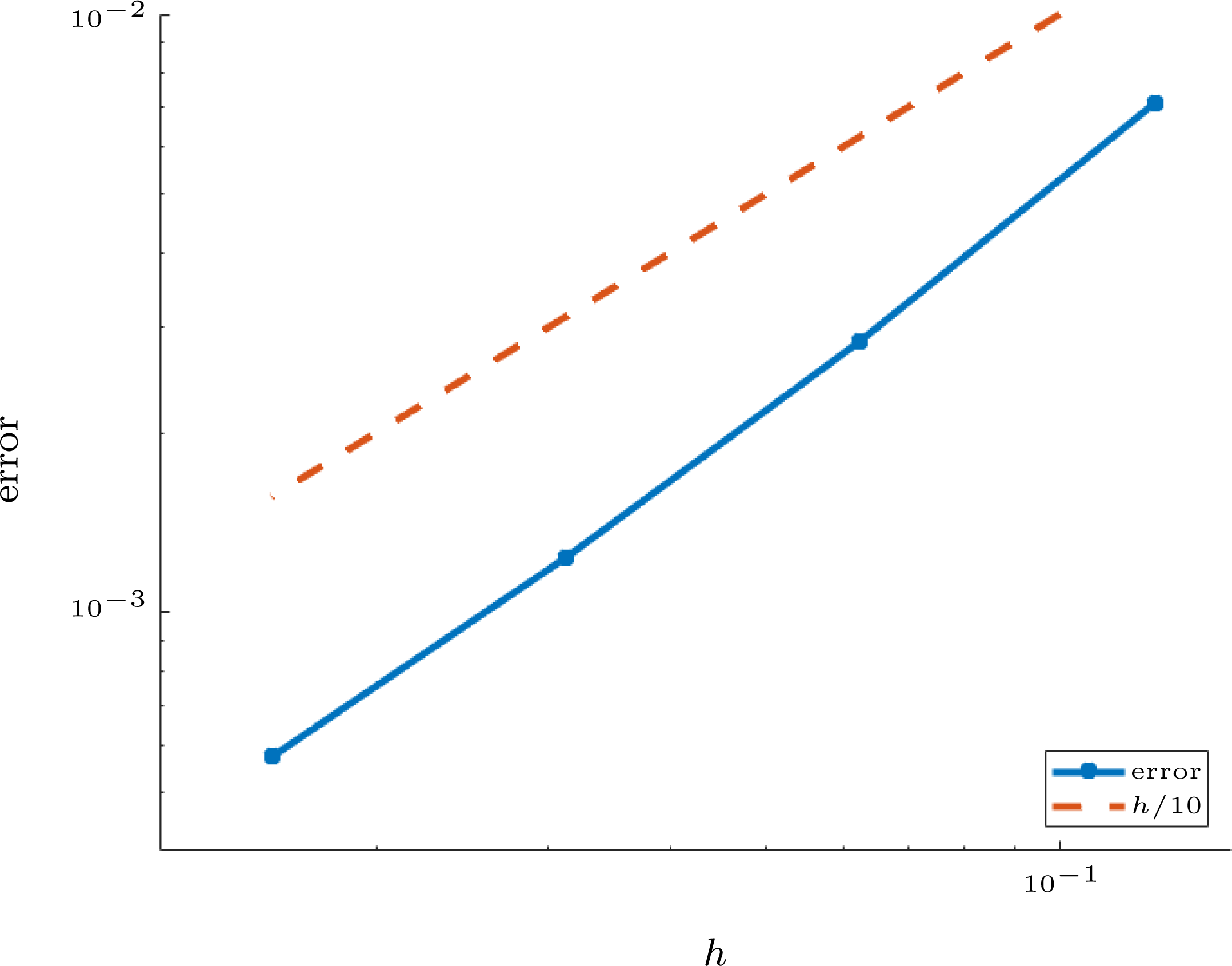
Numerical evidence of second-order convergence of
 $\Vert \boldsymbol{u}_{\text{ref}}(\cdot ,1)-\boldsymbol{u}_{N}^{hk}\Vert _{1}$
(
 $N=1/k$
) with respect to
 $k$
.
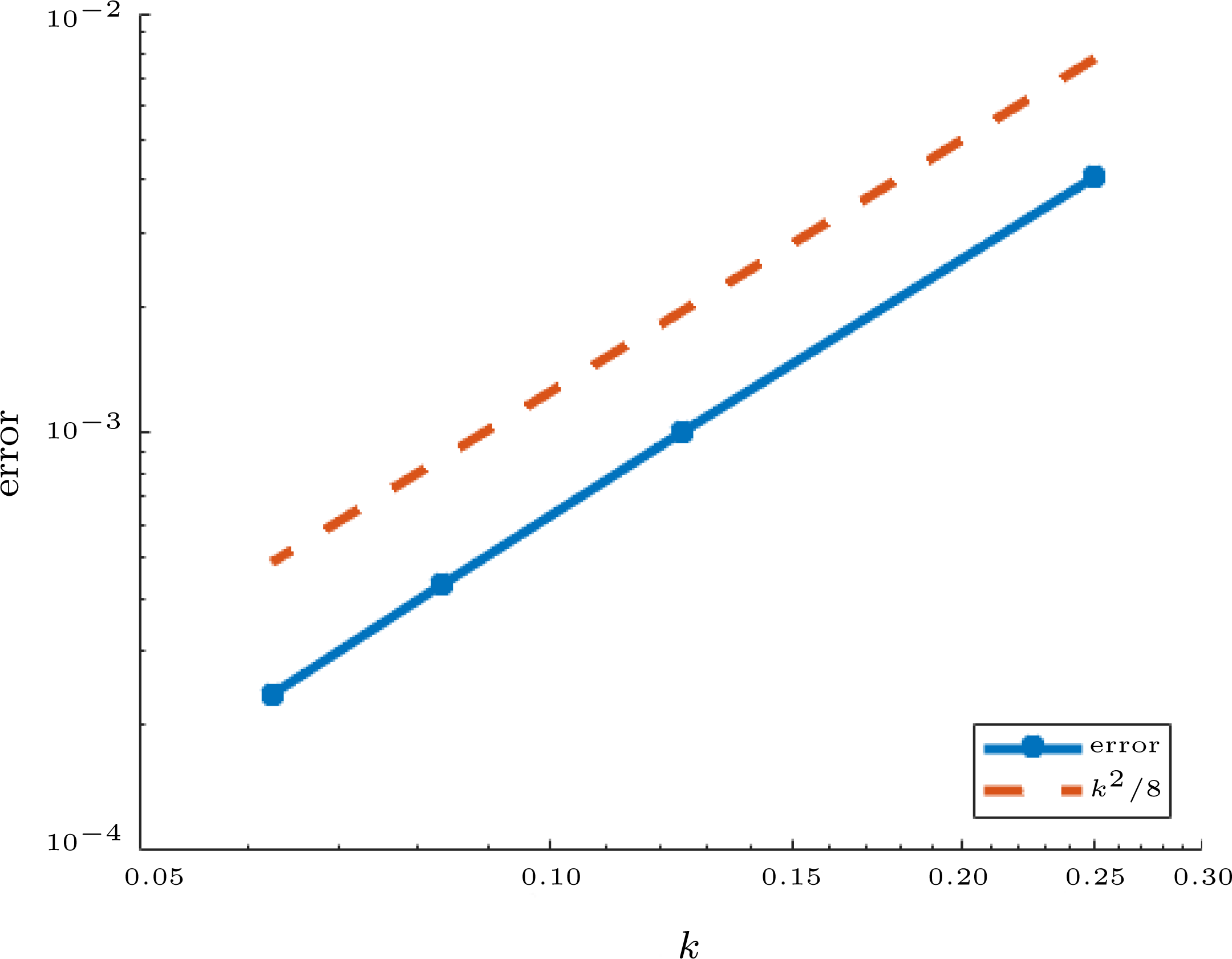
We focus on the numerical convergence orders of the numerical solutions with respect to the mesh-size
 $h$
and the time step-size
 $k$
. Since the true solution is unknown, we use the numerical solution with
 $h=k=1/256$
as the ‘reference’ solution to compute the numerical solution errors. In Figure 8.2, we report the numerical solution errors
 $\Vert \boldsymbol{u}_{\text{ref}}(\cdot ,1)-\boldsymbol{u}_{N}^{hk}\Vert _{1}$
in
 $H^{1}(\unicode[STIX]{x1D6FA};\mathbb{R}^{2})$
-norm (
 $N=1/k$
) for
 $h=1/8,1/16,1/32,1/64$
; a small fixed time step
 $k=1/256$
is used. We observe the linear convergence of the error with respect to the mesh-size
 $h$
. In Figure 8.3, we report the numerical solution errors
 $\Vert \boldsymbol{u}_{\text{ref}}(\cdot ,1)-\boldsymbol{u}_{N}^{hk}\Vert _{1}$
(
 $N=1/k$
) for
 $k=1/4,1/8,1/12,1/16$
; a small fixed mesh-size
 $h=1/256$
is used. We observe the quadratic convergence of the error with respect to the time step
 $k$
. These numerical results match the theoretical error bound (8.20) well.
9 Studies of the dynamic contact problem
In this section we study the dynamic contact problem, Problem 2.10. We first explore the solution existence and uniqueness, then introduce a linear finite element method and derive an optimal order error estimate and, finally, present numerical simulation results. We will use the spaces
 $V$
and
 $H$
defined by (2.3) and (2.5), respectively.
9.1 Solution existence and uniqueness
Recall that
 $\unicode[STIX]{x1D706}_{1\unicode[STIX]{x1D708}}>0$
is the smallest eigenvalue of the eigenvalue problem (7.4). Let
 $\unicode[STIX]{x1D706}_{1\unicode[STIX]{x1D70F}}>0$
be the smallest eigenvalue of the eigenvalue problem
 $$\begin{eqnarray}\boldsymbol{u}\in V,\quad \int _{\unicode[STIX]{x1D6FA}}\unicode[STIX]{x1D73A}(\boldsymbol{u})\cdot \unicode[STIX]{x1D73A}(\boldsymbol{v})\,\text{d}x=\unicode[STIX]{x1D706}\int _{\unicode[STIX]{x1D6E4}_{3}}\boldsymbol{u}_{\unicode[STIX]{x1D70F}}\cdot \boldsymbol{v}_{\unicode[STIX]{x1D70F}}\,\text{d}a\quad \text{for all}~\boldsymbol{v}\in V.\end{eqnarray}$$
The unique solvability of Problem 2.10 is given by the following result.
Theorem 9.1. Assume (2.64)–(2.70) and
 $$\begin{eqnarray}\unicode[STIX]{x1D6FC}_{j_{\unicode[STIX]{x1D708}}}\unicode[STIX]{x1D706}_{1\unicode[STIX]{x1D708}}^{-1}+\unicode[STIX]{x1D6FC}_{j_{\unicode[STIX]{x1D70F}}}\unicode[STIX]{x1D706}_{1\unicode[STIX]{x1D70F}}^{-1}<m_{{\mathcal{A}}}.\end{eqnarray}$$
Then Problem 2.10 has a unique solution with regularity
 $$\begin{eqnarray}\boldsymbol{u}\in H^{1}(0,T;V),\quad \dot{\boldsymbol{u}}\in {\mathcal{W}}\subset C([0,T];L^{2}(\unicode[STIX]{x1D6FA};\mathbb{R}^{d})),\quad \ddot{\boldsymbol{u}}\in {\mathcal{V}}^{\ast }.\end{eqnarray}$$
Proof. Let
 $V_{1}=L^{2}(\unicode[STIX]{x1D6E4}_{3})$
,
 $V_{2}=L^{2}(\unicode[STIX]{x1D6E4}_{3})^{d}$
and define operators
 $\unicode[STIX]{x1D6FE}_{1}\in {\mathcal{L}}(V,V_{1})$
and
 $\unicode[STIX]{x1D6FE}_{2}\in {\mathcal{L}}(V,V_{2})$
by
 $\unicode[STIX]{x1D6FE}_{1}\boldsymbol{v}=v_{\unicode[STIX]{x1D708}}$
and
 $\unicode[STIX]{x1D6FE}_{2}\boldsymbol{v}=\boldsymbol{v}_{\unicode[STIX]{x1D70F}}$
for
 $\boldsymbol{v}\in V$
. Introduce operators
 $A:V\rightarrow V^{\ast }$
and
 ${\mathcal{S}}:{\mathcal{V}}\rightarrow {\mathcal{V}}^{\ast }$
defined by
 $$\begin{eqnarray}\displaystyle \langle A\boldsymbol{u},\boldsymbol{v}\rangle & = & \displaystyle \int _{\unicode[STIX]{x1D6FA}}{\mathcal{A}}\unicode[STIX]{x1D73A}(\boldsymbol{u})\cdot \unicode[STIX]{x1D73A}(\boldsymbol{v})\,\text{d}x\quad \text{for all}~\boldsymbol{u},\boldsymbol{v}\in V,\end{eqnarray}$$
 $$\begin{eqnarray}\displaystyle \langle {\mathcal{S}}\boldsymbol{w}(t),\boldsymbol{v}\rangle & = & \displaystyle \int _{\unicode[STIX]{x1D6FA}}{\mathcal{B}}\biggl(\int _{0}^{t}\unicode[STIX]{x1D73A}(\boldsymbol{w}(s))\,\text{d}s+\boldsymbol{u}_{0}\biggr)\cdot \unicode[STIX]{x1D73A}(\boldsymbol{v})\,\text{d}x\nonumber\\ \displaystyle & & \displaystyle \quad \quad \text{for all}~\boldsymbol{w}\in {\mathcal{V}},~\boldsymbol{v}\in V,~\text{a.e.}~t\in (0,T).\end{eqnarray}$$
In addition, introduce functions
 $j_{1}:V_{1}\rightarrow \mathbb{R}$
,
 $j_{2}:V_{2}\rightarrow \mathbb{R}$
and
 $f:(0,T)\rightarrow V^{\ast }$
given by
 $$\begin{eqnarray}\displaystyle j_{1}(\unicode[STIX]{x1D709}) & = & \displaystyle \int _{\unicode[STIX]{x1D6E4}_{3}}j_{\unicode[STIX]{x1D708}}(\unicode[STIX]{x1D709})\,\text{d}a,\end{eqnarray}$$
 $$\begin{eqnarray}\displaystyle j_{2}(\unicode[STIX]{x1D743}) & = & \displaystyle \int _{\unicode[STIX]{x1D6E4}_{3}}j_{\unicode[STIX]{x1D70F}}(\unicode[STIX]{x1D743})\,\text{d}a,\end{eqnarray}$$
 $$\begin{eqnarray}\displaystyle \langle \boldsymbol{f}(t),\boldsymbol{v}\rangle & = & \displaystyle \int _{\unicode[STIX]{x1D6FA}}\boldsymbol{f}_{0}(t)\cdot \boldsymbol{v}\,\text{d}x+\int _{\unicode[STIX]{x1D6E4}_{2}}\boldsymbol{f}_{2}(t)\cdot \boldsymbol{v}\,\text{d}a\end{eqnarray}$$
for
 $\unicode[STIX]{x1D709}\in V_{1}$
,
 $\unicode[STIX]{x1D743}\in V_{2}$
,
 $\boldsymbol{v}\in V$
, a.e.
 $t\in (0,T)$
. With the above notation we consider the following problem, in terms of the velocity.
Problem 9.2. Find
 $\boldsymbol{w}\in {\mathcal{W}}$
such that
 $$\begin{eqnarray}\displaystyle & & \displaystyle \begin{array}{@{}ll@{}} & \langle \unicode[STIX]{x1D70C}\,\dot{\boldsymbol{w}}(t)+A\boldsymbol{w}(t)+{\mathcal{S}}\boldsymbol{w}(t)-\boldsymbol{f}(t),\boldsymbol{v}-\boldsymbol{w}(t)\rangle \\ & \quad +j_{1}^{0}(w_{\unicode[STIX]{x1D708}}(t);v_{\unicode[STIX]{x1D708}}-w_{\unicode[STIX]{x1D708}}(t))+j_{2}^{0}(\boldsymbol{w}_{\unicode[STIX]{x1D70F}}(t);\boldsymbol{v}_{\unicode[STIX]{x1D70F}}-\boldsymbol{w}_{\unicode[STIX]{x1D70F}}(t))\geq 0\\ & \quad \quad \text{for all}~\boldsymbol{v}\in V,~\text{a.e.}~t\in (0,T),\end{array}\nonumber\\ \displaystyle & & \displaystyle \boldsymbol{w}(0)=\boldsymbol{w}_{0}.\nonumber\end{eqnarray}$$
For an analysis of Problem 9.2, we apply Theorem 6.2 in the functional framework described above. To this end, we check that the hypotheses (6.3)–(6.7) are satisfied.
First, we show that under hypothesis (2.64), the operator
 $A$
defined by (9.4) satisfies hypothesis (6.3) with
 $m_{A}=m_{{\mathcal{A}}}$
. It follows from (2.64(a)), (2.64(c)), and the Hölder inequality that
 $$\begin{eqnarray}\displaystyle \langle A\boldsymbol{u}_{1}-A\boldsymbol{u}_{2},\boldsymbol{v}\rangle & = & \displaystyle \int _{\unicode[STIX]{x1D6FA}}({\mathcal{A}}\unicode[STIX]{x1D73A}(\boldsymbol{u}_{1})-{\mathcal{A}}\unicode[STIX]{x1D73A}(\boldsymbol{u}_{2}))\cdot \unicode[STIX]{x1D73A}(\boldsymbol{v})\,\text{d}x\nonumber\\ \displaystyle & \leq & \displaystyle \Vert {\mathcal{A}}\unicode[STIX]{x1D73A}(\boldsymbol{u}_{1})-{\mathcal{A}}\unicode[STIX]{x1D73A}(\boldsymbol{u}_{2})\Vert _{L^{2}(\unicode[STIX]{x1D6FA};\mathbb{S}^{d})}\Vert \unicode[STIX]{x1D73A}(\boldsymbol{v})\Vert _{L^{2}(\unicode[STIX]{x1D6FA};\mathbb{S}^{d})}\nonumber\\ \displaystyle & \leq & \displaystyle L_{{\mathcal{A}}}\Vert \unicode[STIX]{x1D73A}(\boldsymbol{u}_{1})-\unicode[STIX]{x1D73A}(\boldsymbol{u}_{2})\Vert _{L^{2}(\unicode[STIX]{x1D6FA};\mathbb{S}^{d})}\Vert \unicode[STIX]{x1D73A}(\boldsymbol{v})\Vert _{L^{2}(\unicode[STIX]{x1D6FA};\mathbb{S}^{d})}\nonumber\end{eqnarray}$$
for all
 $\boldsymbol{u}_{1},\boldsymbol{u}_{2},\boldsymbol{v}\in V$
. Hence, we infer that
 $$\begin{eqnarray}\Vert A(t,\boldsymbol{u}_{1})-A(t,\boldsymbol{u}_{2})\Vert _{V^{\ast }}\leq L_{{\mathcal{A}}}\Vert \boldsymbol{u}_{1}-\boldsymbol{u}_{2}\Vert _{V}\end{eqnarray}$$
for all
 $\boldsymbol{u}_{1},\boldsymbol{u}_{2}\in V$
. This inequality shows that
 $A$
is Lipschitz continuous and, in particular, demicontinuous, which proves (6.3(a)).
From (9.9) and (2.64(d)), we also have
 $\Vert A\boldsymbol{u}\Vert _{V^{\ast }}\leq L_{{\mathcal{A}}}\Vert \boldsymbol{u}\Vert _{V}$
for all
 $\boldsymbol{u}\in V$
, which gives (6.3(b)) with
 $a_{0}=0$
and
 $a_{1}=L_{{\mathcal{A}}}$
. Moreover, using (2.64(b)), we obtain
 $$\begin{eqnarray}\displaystyle \langle A\boldsymbol{u}_{1}-A\boldsymbol{u}_{2},\boldsymbol{u}_{1}-\boldsymbol{u}_{2}\rangle & = & \displaystyle \int _{\unicode[STIX]{x1D6FA}}({\mathcal{A}}\unicode[STIX]{x1D73A}(\boldsymbol{u}_{1})-{\mathcal{A}}\unicode[STIX]{x1D73A}(\boldsymbol{u}_{2}))\cdot (\unicode[STIX]{x1D73A}(\boldsymbol{u}_{1})-\unicode[STIX]{x1D73A}(\boldsymbol{u}_{2}))\,\text{d}x\nonumber\\ \displaystyle & \geq & \displaystyle m_{{\mathcal{A}}}\int _{\unicode[STIX]{x1D6FA}}\Vert \unicode[STIX]{x1D73A}(\boldsymbol{u}_{1})-\unicode[STIX]{x1D73A}(\boldsymbol{u}_{2})\Vert _{\mathbb{S}^{d}}^{2}\,\text{d}x\nonumber\\ \displaystyle & = & \displaystyle m_{{\mathcal{A}}}\Vert \boldsymbol{u}_{1}-\boldsymbol{u}_{2}\Vert _{V}^{2}\nonumber\end{eqnarray}$$
for all
 $\boldsymbol{u}_{1},\boldsymbol{u}_{2}\in V$
, which entails (6.3(c)) and completes the proof of (6.3).
Next, using assumption (2.66) and Theorem 3.47 in Migórski, Ochal and Sofonea (Reference Migórski, Ochal and Sofonea2013) it follows that the function
 $j_{1}$
defined by (9.6) satisfies condition (6.4) with
 $\unicode[STIX]{x1D6FC}_{1}=\unicode[STIX]{x1D6FC}_{j_{\unicode[STIX]{x1D708}}}$
,
 $c_{11}=0$
and, moreover,
 $$\begin{eqnarray}j_{1}^{0}(\unicode[STIX]{x1D709};\unicode[STIX]{x1D702})\leq \int _{\unicode[STIX]{x1D6E4}_{3}}j_{\unicode[STIX]{x1D708}}^{0}(\unicode[STIX]{x1D709};\unicode[STIX]{x1D702})\,\text{d}a\quad \text{for all}~\unicode[STIX]{x1D709},\unicode[STIX]{x1D702}\in V_{1}.\end{eqnarray}$$
Assumption (2.67) combined with the same argument shows that the function
 $j_{2}$
defined by (9.7) satisfies condition (6.4) with
 $\unicode[STIX]{x1D6FC}_{2}=\unicode[STIX]{x1D6FC}_{j_{\unicode[STIX]{x1D70F}}}$
,
 $c_{12}=0$
and, in addition,
 $$\begin{eqnarray}j_{2}^{0}(\unicode[STIX]{x1D743};\boldsymbol{\unicode[STIX]{x1D702}})\leq \int _{\unicode[STIX]{x1D6E4}_{3}}j_{\unicode[STIX]{x1D70F}}^{0}(\unicode[STIX]{x1D743};\boldsymbol{\unicode[STIX]{x1D702}})\,\text{d}a\quad \text{for all}~\unicode[STIX]{x1D743},\boldsymbol{\unicode[STIX]{x1D702}}\in V_{2}.\end{eqnarray}$$
It is easy to see that the smallness condition (6.5) follows from (9.2).
Moreover, the hypothesis (2.65) implies that the operator
 ${\mathcal{S}}$
defined by (9.5) satisfies conditions (6.6). Indeed, let
 $\boldsymbol{w}_{1},\boldsymbol{w}_{2}\in {\mathcal{V}}$
,
 $\boldsymbol{v}\in V$
and
 $t\in (0,T)$
. Using (2.65) and the Hölder inequality, we have
 $$\begin{eqnarray}\displaystyle & & \displaystyle \biggl|\biggl({\mathcal{B}}\biggl(\int _{0}^{t}\unicode[STIX]{x1D73A}(\boldsymbol{w}_{1}(s))\,\text{d}s+\boldsymbol{u}_{0}\biggr)-{\mathcal{B}}\biggl(\int _{0}^{t}\unicode[STIX]{x1D73A}(\boldsymbol{w}_{2}(s))\,\text{d}s+\boldsymbol{u}_{0}\biggr),\unicode[STIX]{x1D73A}(\boldsymbol{v})\biggr)_{L^{2}(\unicode[STIX]{x1D6FA};\mathbb{S}^{d})}\biggr|\nonumber\\ \displaystyle & & \displaystyle \quad ~~\leq \biggl\|{\mathcal{B}}\biggl(\int _{0}^{t}\unicode[STIX]{x1D73A}(\boldsymbol{w}_{1}(s))\,\text{d}s+\boldsymbol{u}_{0}\biggr)-{\mathcal{B}}\biggl(\int _{0}^{t}\unicode[STIX]{x1D73A}(\boldsymbol{w}_{2}(s))\,\text{d}s+\boldsymbol{u}_{0}\biggr)\biggr\|_{L^{2}(\unicode[STIX]{x1D6FA};\mathbb{S}^{d})}\Vert \boldsymbol{v}\Vert _{V}\nonumber\\ \displaystyle & & \displaystyle \quad ~~\leq L_{{\mathcal{B}}}\int _{0}^{t}\Vert \unicode[STIX]{x1D73A}(\boldsymbol{w}_{1}(s)-\boldsymbol{w}_{2}(s))\Vert _{L^{2}(\unicode[STIX]{x1D6FA};\mathbb{S}^{d})}\,\text{d}s\,\Vert \boldsymbol{v}\Vert _{V}\nonumber\\ \displaystyle & & \displaystyle \quad ~~=L_{{\mathcal{B}}}\,\biggl(\int _{0}^{t}\Vert \boldsymbol{w}_{1}(s)-\boldsymbol{w}_{2}(s)\Vert _{V}\,\text{d}s\biggr)\Vert \boldsymbol{v}\Vert _{V}.\nonumber\end{eqnarray}$$
Therefore
 $$\begin{eqnarray}|({\mathcal{S}}\boldsymbol{w}_{1}(t)-{\mathcal{S}}\boldsymbol{w}_{2}(t),\unicode[STIX]{x1D73A}(\boldsymbol{v}))_{L^{2}(\unicode[STIX]{x1D6FA};\mathbb{S}^{d})}|\leq L_{{\mathcal{B}}}\biggl(\int _{0}^{t}\Vert \boldsymbol{w}_{1}(s)-\boldsymbol{w}_{2}(s)\Vert _{V}\,\text{d}s\biggr)\Vert \boldsymbol{v}\Vert _{V},\end{eqnarray}$$
which implies that the operator
 ${\mathcal{S}}$
satisfies (6.6) with
 $c_{S}=L_{{\mathcal{B}}}$
.
Finally, condition (6.7) is a consequence of assumptions (2.69), (2.70) and definition (9.8).
Since all the hypotheses of Theorem 6.2 are satisfied, we conclude that Problem 9.2 has a unique solution
 $\boldsymbol{w}\in {\mathcal{W}}$
. Then, we define the function
 $\boldsymbol{u}:[0,T]\rightarrow V$
by
 $$\begin{eqnarray}\boldsymbol{u}(t)=\int _{0}^{t}\boldsymbol{w}(s)\,\text{d}s+\boldsymbol{u}_{0},\quad t\in [0,T].\end{eqnarray}$$
It follows from inequalities (9.10), (9.11) that
 $\boldsymbol{u}$
is a solution to Problem 2.10. This completes the proof of the existence part of the theorem. The regularity (9.3) is a consequence of the regularity
 $\boldsymbol{w}\in {\mathcal{W}}$
, assumption
 $\boldsymbol{u}_{0}\in V$
, and equality (9.12).
Finally, the uniqueness part of Theorem 9.1 is a consequence of the smallness assumption (9.2) combined with a standard Gronwall argument.◻
9.2 Numerical analysis of the problem
We now proceed with the discretization of Problem 2.10. We use the symbol
 $\boldsymbol{w}:=\dot{\boldsymbol{u}}$
to denote the velocity field and express the fully discrete scheme in terms of approximate velocities. As in Section 8.2, we use the linear finite element space
 $V^{h}$
and a uniform partition of the time interval
 $[0,T]$
with step-size
 $k=T/N$
and partition points
 $t_{n}=n\,k$
,
 $0\leq n\leq N$
. Corresponding to (6.17), we assume
 $$\begin{eqnarray}\boldsymbol{f}_{0}\in C([0,T];L^{2}(\unicode[STIX]{x1D6FA};\mathbb{R}^{d})),\quad \boldsymbol{f}_{2}\in C([0,T];L^{2}(\unicode[STIX]{x1D6E4}_{2};\mathbb{R}^{d})).\end{eqnarray}$$
Denote
 $\boldsymbol{f}_{0,n}=\boldsymbol{f}_{0}(t_{n})$
,
 $\boldsymbol{f}_{2,n}=\boldsymbol{f}_{2}(t_{n})$
. Let
 $\boldsymbol{u}_{0}^{h},\boldsymbol{w}_{0}^{h}\in V^{h}$
be appropriate approximations of the initial values
 $\boldsymbol{u}_{0},\boldsymbol{w}_{0}$
. Then the fully discrete numerical method is as follows.
Problem 9.3. Find
 $\boldsymbol{w}^{hk}=\{\boldsymbol{w}_{n}^{hk_{}^{}\}}\subset V^{h}$
such that for
 $1\leq n\leq N$
,
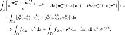 $$\begin{eqnarray}\displaystyle & & \displaystyle \int _{\unicode[STIX]{x1D6FA}}\biggl[\unicode[STIX]{x1D70C}\,\displaystyle \frac{\boldsymbol{w}_{n}^{hk}-\boldsymbol{w}_{n-1}^{hk}}{k}\cdot \boldsymbol{v}^{h}+{\mathcal{A}}\unicode[STIX]{x1D73A}(\boldsymbol{w}_{n}^{hk})\cdot \unicode[STIX]{x1D73A}(\boldsymbol{v}^{h})+{\mathcal{B}}\unicode[STIX]{x1D73A}(\boldsymbol{u}_{n}^{hk})\cdot \unicode[STIX]{x1D73A}(\boldsymbol{v}^{h})\biggr]\,\text{d}x\nonumber\\ \displaystyle & & \displaystyle \quad +\int _{\unicode[STIX]{x1D6E4}_{3}}[j_{\unicode[STIX]{x1D708}}^{0}(w_{n,\unicode[STIX]{x1D708}}^{hk};v_{\unicode[STIX]{x1D708}}^{h})+j_{\unicode[STIX]{x1D70F}}^{0}(\boldsymbol{w}_{n,\unicode[STIX]{x1D70F}}^{hk};\boldsymbol{v}_{\unicode[STIX]{x1D70F}}^{h})]\,\text{d}a\nonumber\\ \displaystyle & & \displaystyle \quad \quad \geq \int _{\unicode[STIX]{x1D6FA}}\boldsymbol{f}_{0,n}\cdot \boldsymbol{v}^{h}\,\text{d}x+\int _{\unicode[STIX]{x1D6E4}_{2}}\boldsymbol{f}_{2,n}\cdot \boldsymbol{v}^{h}\,\text{d}a\quad \text{for all}~\boldsymbol{v}^{h}\in V^{h},\end{eqnarray}$$
and
 $$\begin{eqnarray}\boldsymbol{w}_{0}^{hk}=\boldsymbol{w}_{0}^{h}.\end{eqnarray}$$
Here
 $$\begin{eqnarray}\boldsymbol{u}_{n}^{hk}=\boldsymbol{u}_{0}^{h}+k\mathop{\sum }_{i=0}^{n-1}\boldsymbol{w}_{i}^{hk}\end{eqnarray}$$
and
 $\boldsymbol{u}_{0}^{h}\in V^{h}$
is an approximation of
 $\boldsymbol{u}_{0}$
.
The main goal in this subsection is to derive an error estimate for the numerical solution defined by Problem 9.3. To this end, we will apply the error bound (6.53), which still holds when
 $$\begin{eqnarray}j_{1}^{0}(\unicode[STIX]{x1D6FE}_{1}w_{n}^{hk};\unicode[STIX]{x1D6FE}_{1}v^{h}),\quad j_{2}^{0}(\unicode[STIX]{x1D6FE}_{2}w_{n}^{hk};\unicode[STIX]{x1D6FE}_{2}v^{h})\end{eqnarray}$$
in (6.21) are replaced by
 $$\begin{eqnarray}\int _{\unicode[STIX]{x1D6E4}_{3}}j_{\unicode[STIX]{x1D708}}^{0}(w_{n,\unicode[STIX]{x1D708}}^{hk};v_{\unicode[STIX]{x1D708}}^{h})\,\text{d}a,\quad \int _{\unicode[STIX]{x1D6E4}_{3}}j_{\unicode[STIX]{x1D70F}}^{0}(\boldsymbol{w}_{n,\unicode[STIX]{x1D70F}}^{hk};\boldsymbol{v}_{\unicode[STIX]{x1D70F}}^{h})\,\text{d}a\end{eqnarray}$$
as in (9.14). We assume the solution regularity
 $$\begin{eqnarray}\boldsymbol{u}\in C^{1}([0,T];H^{2}(\unicode[STIX]{x1D6FA};\mathbb{R}^{d}))\cap H^{2}(0,T;V)\cap H^{3}(0,T;V^{\ast }).\end{eqnarray}$$
Note that (9.17) implies the following counterpart of (6.30):
 $$\begin{eqnarray}\boldsymbol{w}\in C([0,T];V)\cap H^{2}(0,T;V^{\ast }).\end{eqnarray}$$
We will additionally assume
 $$\begin{eqnarray}\displaystyle \unicode[STIX]{x1D748}\unicode[STIX]{x1D742} & \in & \displaystyle C([0,T];L^{2}(\unicode[STIX]{x1D6E4};\mathbb{R}^{d})),\end{eqnarray}$$
 $$\begin{eqnarray}\displaystyle \dot{\boldsymbol{u}}|_{\unicode[STIX]{x1D6E4}_{3,i}} & \in & \displaystyle C([0,T];H^{2}(\unicode[STIX]{x1D6E4}_{3,i};\mathbb{R}^{d}),\quad 1\leq i\leq i_{3}.\end{eqnarray}$$
Observe that if
 ${\mathcal{A}}$
and
 ${\mathcal{B}}$
are smooth, then (9.18) follows from the condition
 $\boldsymbol{u}\in C^{1}([0,T];H^{1}(\unicode[STIX]{x1D6FA};\mathbb{R}^{d}))$
implied by (9.17).
We first consider the residual-type term defined by (6.35), which takes the following form for Problem 9.3:
 $$\begin{eqnarray}\displaystyle R_{n}(\boldsymbol{v}) & = & \displaystyle \langle \unicode[STIX]{x1D70C}\,\dot{\boldsymbol{w}}_{n},\boldsymbol{v}\rangle +\int _{\unicode[STIX]{x1D6FA}}\unicode[STIX]{x1D748}_{n}\cdot \unicode[STIX]{x1D73A}(\boldsymbol{v})\,\text{d}x+\int _{\unicode[STIX]{x1D6E4}_{3}}[j_{\unicode[STIX]{x1D708}}^{0}(w_{n,\unicode[STIX]{x1D708}};v_{\unicode[STIX]{x1D708}})+j_{\unicode[STIX]{x1D70F}}^{0}(\boldsymbol{w}_{n,\unicode[STIX]{x1D70F}};\boldsymbol{v}_{\unicode[STIX]{x1D70F}})]\,\text{d}a\nonumber\\ \displaystyle & & \displaystyle -\,\int _{\unicode[STIX]{x1D6FA}}\boldsymbol{f}_{0,n}\cdot \boldsymbol{v}\,\text{d}x-\int _{\unicode[STIX]{x1D6E4}_{2}}\boldsymbol{f}_{2,n}\cdot \boldsymbol{v}\,\text{d}a,\end{eqnarray}$$
where
 $$\begin{eqnarray}\unicode[STIX]{x1D748}_{n}:=\unicode[STIX]{x1D748}(t_{n})={\mathcal{A}}\unicode[STIX]{x1D73A}(\boldsymbol{w}_{n})+{\mathcal{B}}\unicode[STIX]{x1D73A}(\boldsymbol{u}_{n}),\quad 1\leq n\leq N.\end{eqnarray}$$
Recall the space
 $\tilde{U}$
defined in (7.20). In the defining inequality (2.71), we take
 $\boldsymbol{v}\in \tilde{U}$
to obtain
 $$\begin{eqnarray}\displaystyle \langle \unicode[STIX]{x1D70C}\,\dot{\boldsymbol{w}}(t),\boldsymbol{v}\rangle +\int _{\unicode[STIX]{x1D6FA}}\unicode[STIX]{x1D748}(t)\cdot \unicode[STIX]{x1D73A}(\boldsymbol{v})\,\text{d}x & = & \displaystyle \int _{\unicode[STIX]{x1D6FA}}\boldsymbol{f}_{0}(t)\cdot \boldsymbol{v}\,\text{d}x+\int _{\unicode[STIX]{x1D6E4}_{2}}\boldsymbol{f}_{2}(t)\cdot \boldsymbol{v}\,\text{d}a\nonumber\\ \displaystyle & & \displaystyle \qquad \text{for all}~\boldsymbol{v}\in \tilde{U} .\end{eqnarray}$$
As in (7.22) and (7.23), we derive from (9.22) that for a.e.
 $t\in (0,T)$
,
 $$\begin{eqnarray}\unicode[STIX]{x1D70C}\,\dot{\boldsymbol{w}}(t)-\text{Div}\,\unicode[STIX]{x1D748}(t)=\boldsymbol{f}_{0}(t)\quad \text{a.e. in }\unicode[STIX]{x1D6FA}\end{eqnarray}$$
and
 $$\begin{eqnarray}\unicode[STIX]{x1D748}(t)\unicode[STIX]{x1D742}=\boldsymbol{f}_{2}(t)\quad \text{a.e. on }\unicode[STIX]{x1D6E4}_{2}.\end{eqnarray}$$
Now we multiply the equation (9.23) by an arbitrary function
 $\boldsymbol{v}\in V$
and integrate over
 $\unicode[STIX]{x1D6FA}$
:
 $$\begin{eqnarray}\langle \unicode[STIX]{x1D70C}\,\dot{\boldsymbol{w}}(t),\boldsymbol{v}\rangle -\int _{\unicode[STIX]{x1D6FA}}\text{Div}\,\unicode[STIX]{x1D748}(t)\cdot \boldsymbol{v}\,\text{d}x=\int _{\unicode[STIX]{x1D6FA}}\boldsymbol{f}_{0}(t)\cdot \boldsymbol{v}\,\text{d}x.\end{eqnarray}$$
Perform an integration by parts on the second integral and use (9.24) to get
 $$\begin{eqnarray}\displaystyle & & \displaystyle \langle \unicode[STIX]{x1D70C}\,\dot{\boldsymbol{w}}(t),\boldsymbol{v}\rangle +\int _{\unicode[STIX]{x1D6FA}}\unicode[STIX]{x1D748}(t)\cdot \unicode[STIX]{x1D73A}(\boldsymbol{v})\,\text{d}x-\int _{\unicode[STIX]{x1D6E4}_{3}}\unicode[STIX]{x1D748}(t)\unicode[STIX]{x1D742}\cdot \boldsymbol{v}\,\text{d}a\nonumber\\ \displaystyle & & \displaystyle \quad =\int _{\unicode[STIX]{x1D6FA}}\boldsymbol{f}_{0}(t)\cdot \boldsymbol{v}\,\text{d}x+\int _{\unicode[STIX]{x1D6E4}_{2}}\boldsymbol{f}_{2}(t)\cdot \boldsymbol{v}\,\text{d}a\quad \text{for all}~\boldsymbol{v}\in V,\text{ a.e. }t\in (0,T).\end{eqnarray}$$
Thus, the term
 $R_{n}(\cdot )$
given in (9.20) can be simplified to
 $$\begin{eqnarray}R_{n}(\boldsymbol{v})=\int _{\unicode[STIX]{x1D6E4}_{3}}[\unicode[STIX]{x1D748}_{n}\unicode[STIX]{x1D742}\cdot \boldsymbol{v}+j_{\unicode[STIX]{x1D708}}^{0}(w_{n,\unicode[STIX]{x1D708}};v_{\unicode[STIX]{x1D708}})+j_{\unicode[STIX]{x1D70F}}^{0}(\boldsymbol{w}_{n,\unicode[STIX]{x1D70F}};\boldsymbol{v}_{\unicode[STIX]{x1D70F}})]\,\text{d}a,\quad \boldsymbol{v}\in V.\end{eqnarray}$$
Therefore,
 $$\begin{eqnarray}|R_{n}(\boldsymbol{v})|\leq c\,\Vert \boldsymbol{v}\Vert _{L^{2}(\unicode[STIX]{x1D6E4}_{3};\mathbb{R}^{d})}\quad \text{for all}~\boldsymbol{v}\in V.\end{eqnarray}$$
Hence, from (6.53) and (6.52), we have
 $$\begin{eqnarray}\displaystyle & & \displaystyle \max _{1\leq n\leq N}\Vert \boldsymbol{w}_{n}-\boldsymbol{w}_{n}^{hk}\Vert _{H}^{2}+k\mathop{\sum }_{n=1}^{N}\Vert \boldsymbol{w}_{n}-\boldsymbol{w}_{n}^{hk}\Vert _{V}^{2}\nonumber\\ \displaystyle & & \displaystyle \quad \leq c\,k^{2}(\Vert \ddot{\boldsymbol{w}}\Vert _{L^{2}(0,T;V^{\ast })}^{2}+\Vert \boldsymbol{w}\Vert _{H^{1}(0,T;V)}^{2})\nonumber\\ \displaystyle & & \displaystyle \quad \quad +c(\Vert \boldsymbol{w}_{0}-\boldsymbol{w}_{0}^{h}\Vert _{H}^{2}+k\,\Vert \boldsymbol{w}_{0}-\boldsymbol{w}_{0}^{h}\Vert _{V}^{2})+c\,\max _{1\leq n\leq N}\tilde{E}_{n},\end{eqnarray}$$
where
 $$\begin{eqnarray}\displaystyle \tilde{E}_{n}=\inf _{\mathbf{v}_{i}^{h}\in V^{h},\,1\leq i\leq n} & & \displaystyle \Bigg\{k\mathop{\sum }_{i=1}^{n}\Vert \boldsymbol{w}_{i}-\boldsymbol{v}_{i}^{h}\Vert _{V}^{2}+\left[k\mathop{\sum }_{i=1}^{n}\Vert \boldsymbol{w}_{i}-\boldsymbol{v}_{i}^{h}\Vert _{L^{2}(\unicode[STIX]{x1D6E4}_{3};\mathbb{R}^{d})}^{2}\right]^{1/2}\nonumber\\ \displaystyle & & \displaystyle +k^{-1}\mathop{\sum }_{i=1}^{n-1}\Vert (\boldsymbol{w}_{i}-\boldsymbol{v}_{i}^{h})-(\boldsymbol{w}_{i+1}-\boldsymbol{v}_{i+1}^{h})\Vert _{V^{\ast }}^{2}\nonumber\\ \displaystyle & & \displaystyle +\Vert \boldsymbol{w}_{1}-\boldsymbol{v}_{1}^{h}\Vert _{H}^{2}+\Vert \boldsymbol{w}_{n}-\boldsymbol{v}_{n}^{h}\Vert _{H}^{2}\Bigg\}.\end{eqnarray}$$
Note that (9.17) implies
 $$\begin{eqnarray}\boldsymbol{w}\in C([0,T];H^{2}(\unicode[STIX]{x1D6FA};\mathbb{R}^{d}))\cap H^{1}(0,T;V)\cap H^{2}(0,T;V^{\ast }).\end{eqnarray}$$
This in particular implies
 $$\begin{eqnarray}\boldsymbol{w}_{0}\in H^{2}(\unicode[STIX]{x1D6FA};\mathbb{R}^{d}).\end{eqnarray}$$
Let
 $\boldsymbol{w}_{0}^{h}\in V^{h}$
be the finite element interpolant or projection of
 $\boldsymbol{w}_{0}$
. Then
 $$\begin{eqnarray}\Vert \boldsymbol{w}_{0}-\boldsymbol{w}_{0}^{h}\Vert _{H}\leq c\,h^{2}\Vert \boldsymbol{w}_{0}\Vert _{H^{2}(\unicode[STIX]{x1D6FA})^{d}}.\end{eqnarray}$$
Let
 $\boldsymbol{v}_{i}^{h}\in V^{h}$
be the finite element interpolant of
 $\boldsymbol{w}_{i}$
,
 $1\leq i\leq N$
. Note that
 $(\boldsymbol{v}_{i}^{h}-\boldsymbol{v}_{i+1}^{h})$
is the finite element interpolant of
 $(\boldsymbol{w}_{i}-\boldsymbol{w}_{i+1})$
,
 $0\leq i\leq N-1$
. Moreover,
 $\boldsymbol{v}_{i}^{h}$
interpolates
 $\boldsymbol{w}_{i}$
on the boundary
 $\unicode[STIX]{x1D6E4}_{3}$
. Then, from the finite element interpolation theory, under the stated solution regularities, we obtain from (9.28) and (9.29) the following optimal order error estimate:
 $$\begin{eqnarray}\max _{1\leq n\leq N}\Vert \boldsymbol{w}_{n}-\boldsymbol{w}_{n}^{hk}\Vert _{H}+\left[k\mathop{\sum }_{n=1}^{N}\Vert \boldsymbol{w}_{n}-\boldsymbol{w}_{n}^{hk}\Vert _{V}^{2}\right]^{1/2}\leq c(k+h),\end{eqnarray}$$
for a constant
 $c>0$
depending on
 $\boldsymbol{w}$
, but not on the discretization parameters
 $k$
and
 $h$
.
We now turn to an error estimate for the displacement. We note that (9.17) implies
 $$\begin{eqnarray}\ddot{\boldsymbol{u}}\in L^{2}(0,T;V),\quad \boldsymbol{u}_{0}\in H^{2}(\unicode[STIX]{x1D6FA};\mathbb{R}^{d}).\end{eqnarray}$$
From (9.12) and (9.16), we have
 $$\begin{eqnarray}\boldsymbol{u}_{n}-\boldsymbol{u}_{n}^{hk}=\boldsymbol{u}_{0}-\boldsymbol{u}_{0}^{hk}+k\mathop{\sum }_{i=0}^{n-1}(\boldsymbol{w}_{i}-\boldsymbol{w}_{i}^{hk})+\mathop{\sum }_{i=0}^{n-1}\int _{t_{i}}^{t_{i+1}}(\boldsymbol{w}(t)-\boldsymbol{w}_{i})\,\text{d}t.\end{eqnarray}$$
Then,
 $$\begin{eqnarray}\displaystyle \Vert \boldsymbol{u}_{n}-\boldsymbol{u}_{n}^{hk}\Vert _{V} & \leq & \displaystyle \Vert \boldsymbol{u}_{0}-\boldsymbol{u}_{0}^{hk}\Vert _{V}+k\mathop{\sum }_{i=0}^{n-1}\Vert \boldsymbol{w}_{i}-\boldsymbol{w}_{i}^{hk}\Vert _{V}\nonumber\\ \displaystyle & & \displaystyle +\,\mathop{\sum }_{i=0}^{n-1}\int _{t_{i}}^{t_{i+1}}\Vert \boldsymbol{w}(t)-\boldsymbol{w}_{i}\Vert _{V}\,\text{d}t.\end{eqnarray}$$
From
 $$\begin{eqnarray}\boldsymbol{w}(t)-\boldsymbol{w}_{i}=\int _{t_{i}}^{t}\dot{\boldsymbol{w}}(s)\,\text{d}s,\end{eqnarray}$$
we find
 $$\begin{eqnarray}\Vert \boldsymbol{w}(t)-\boldsymbol{w}_{i}\Vert _{V}\leq \int _{t_{i}}^{t_{i+1}}\Vert \dot{\boldsymbol{w}}(s)\Vert _{V}\,\text{d}s,\quad t\in [t_{i},t_{i+1}],\end{eqnarray}$$
and then
 $$\begin{eqnarray}\mathop{\sum }_{i=0}^{n-1}\int _{t_{i}}^{t_{i+1}}\Vert \boldsymbol{w}(t)-\boldsymbol{w}_{i}\Vert _{V}\,\,\text{d}t\leq k\,\Vert \dot{\boldsymbol{w}}\Vert _{L^{1}(0,T;V)}.\end{eqnarray}$$
If
 $\boldsymbol{u}_{0}^{h}\in V^{h}$
is the finite element interpolant or projection of
 $\boldsymbol{u}_{0}$
, then
 $$\begin{eqnarray}\Vert \boldsymbol{u}_{0}-\boldsymbol{u}_{0}^{hk}\Vert _{V}\leq c\,h\,\Vert \boldsymbol{u}_{0}\Vert _{H^{2}(\unicode[STIX]{x1D6FA};\mathbb{R}^{d})}.\end{eqnarray}$$
Thus, from (9.32), we have
 $$\begin{eqnarray}\displaystyle \Vert \boldsymbol{u}_{n}-\boldsymbol{u}_{n}^{hk}\Vert _{V}\leq k\mathop{\sum }_{i=0}^{n-1}\Vert \boldsymbol{w}_{i}-\boldsymbol{w}_{i}^{hk}\Vert _{V}+c(h\,\Vert \boldsymbol{u}_{0}\Vert _{H^{2}(\unicode[STIX]{x1D6FA};\mathbb{R}^{d})}+k\,\Vert \ddot{\boldsymbol{u}}\Vert _{L^{1}(0,T;V)}). & & \displaystyle\end{eqnarray}$$
Apply the Cauchy–Schwarz inequality and use (9.31) and (9.30):
 $$\begin{eqnarray}\displaystyle k\mathop{\sum }_{i=1}^{n}\Vert \boldsymbol{w}_{i}-\boldsymbol{w}_{i}^{hk}\Vert _{V} & \leq & \displaystyle (k\,n)^{1/2}\left[k\mathop{\sum }_{i=1}^{n}\Vert \boldsymbol{w}_{i}-\boldsymbol{w}_{i}^{hk}\Vert _{V}^{2}\right]^{1/2}\nonumber\\ \displaystyle & \leq & \displaystyle c(k+h).\nonumber\end{eqnarray}$$
Therefore, from (9.33) we derive the optimal order error estimate
 $$\begin{eqnarray}\max _{0\leq n\leq N}\Vert \boldsymbol{u}_{n}-\boldsymbol{u}_{n}^{hk}\Vert _{V}\leq c(k+h).\end{eqnarray}$$
9.3 A numerical example
In this subsection we report numerical results on a dynamic frictional contact problem following Barboteu, Bartosz, Han and Janiczko (Reference Barboteu, Bartosz, Han and Janiczko2015). The contact problem represents a variant of Problem 2.9 and can be formulated as follows.
Problem 9.4. Find a displacement field
 $\boldsymbol{u}:\unicode[STIX]{x1D6FA}\times [0,T]\rightarrow \mathbb{R}^{d}$
and a stress field
 $\unicode[STIX]{x1D748}:\unicode[STIX]{x1D6FA}\times [0,T]\rightarrow \mathbb{S}^{d}$
such that
 $$\begin{eqnarray}\displaystyle \unicode[STIX]{x1D748}(t)={\mathcal{A}}\unicode[STIX]{x1D73A}(\dot{\boldsymbol{u}}(t))+{\mathcal{B}}\unicode[STIX]{x1D73A}(\boldsymbol{u}(t))\quad & \text{in}~\unicode[STIX]{x1D6FA}, & \displaystyle\end{eqnarray}$$
 $$\begin{eqnarray}\displaystyle \unicode[STIX]{x1D70C}\,\ddot{\boldsymbol{u}}(t)=\text{Div}\,\unicode[STIX]{x1D748}(t)+\boldsymbol{f}_{0}(t)\quad & \text{in}~\unicode[STIX]{x1D6FA}, & \displaystyle\end{eqnarray}$$
 $$\begin{eqnarray}\displaystyle \boldsymbol{u}(t)=\mathbf{0}\quad & \text{on}~\unicode[STIX]{x1D6E4}_{1}, & \displaystyle\end{eqnarray}$$
 $$\begin{eqnarray}\displaystyle \unicode[STIX]{x1D748}(t)\unicode[STIX]{x1D742}=\boldsymbol{f}_{2}(t)\quad & \text{on}~\unicode[STIX]{x1D6E4}_{2}, & \displaystyle\end{eqnarray}$$
 $$\begin{eqnarray}\displaystyle u_{\unicode[STIX]{x1D708}}=0\quad & \text{on}~\unicode[STIX]{x1D6E4}_{3}, & \displaystyle\end{eqnarray}$$
 $$\begin{eqnarray}\displaystyle |\unicode[STIX]{x1D748}_{\unicode[STIX]{x1D70F}}|\leq \unicode[STIX]{x1D707}(\Vert \dot{\boldsymbol{u}}_{\unicode[STIX]{x1D70F}}\Vert ),~~-\unicode[STIX]{x1D748}_{\unicode[STIX]{x1D70F}}=\unicode[STIX]{x1D707}(\Vert \dot{\boldsymbol{u}}_{\unicode[STIX]{x1D70F}}\Vert )\displaystyle \frac{\dot{\boldsymbol{u}}_{\unicode[STIX]{x1D70F}}}{\Vert \dot{\boldsymbol{u}}_{\unicode[STIX]{x1D70F}}\Vert }~\text{if}~\dot{\boldsymbol{u}}_{\unicode[STIX]{x1D70F}}\neq \mathbf{0}\quad & \text{on}~\unicode[STIX]{x1D6E4}_{3}, & \displaystyle\end{eqnarray}$$
for all
 $t\in [0,T]$
, and
 $$\begin{eqnarray}\boldsymbol{u}(0)=\boldsymbol{u}_{0},\quad \dot{\boldsymbol{u}}(0)=\boldsymbol{w}_{0}\quad \text{in}~\unicode[STIX]{x1D6FA}.\end{eqnarray}$$
The difference between Problems 2.9 and 9.4 lies in the contact boundary condition. The condition (2.58) is replaced by the bilateral contact condition (9.39). In the subdifferential friction law (2.59), we choose
 $$\begin{eqnarray}j_{\unicode[STIX]{x1D70F}}(\unicode[STIX]{x1D743})=\int _{0}^{\Vert \boldsymbol{\unicode[STIX]{x1D709}}\Vert }\unicode[STIX]{x1D707}(s)\,\text{d}s,\quad \unicode[STIX]{x1D743}\in \mathbb{R}^{d}.\end{eqnarray}$$
Here,
 $\unicode[STIX]{x1D707}:[0,\infty )\rightarrow \mathbb{R}_{+}$
represents the friction bound and is assumed to satisfy the following conditions:
 $$\begin{eqnarray}\left.\begin{array}{@{}ll@{}}\text{(a) } & \unicode[STIX]{x1D707}\text{ is continuous;}\\[3.0pt] \text{(b) } & |\unicode[STIX]{x1D707}(s)|\leq c(1+s)\text{ for all }s\geq 0,~c>0;\\[3.0pt] \text{(c) } & \unicode[STIX]{x1D707}(s_{1})-\unicode[STIX]{x1D707}(s_{2})\geq -\unicode[STIX]{x1D706}(s_{1}-s_{2})\text{ for all }s_{1}>s_{2}\geq 0\text{ with }\unicode[STIX]{x1D706}>0.\end{array}\right\}\end{eqnarray}$$
In the study of Problem 2.9, we use the function space
 $$\begin{eqnarray}\widetilde{V}=\{\boldsymbol{v}\in V\mid v_{\unicode[STIX]{x1D708}}=0\text{ a.e. on }\unicode[STIX]{x1D6E4}_{3}\}.\end{eqnarray}$$
Moreover, besides (9.43) we assume that (2.64), (2.65), (2.69) and (2.70) hold. Then, the weak formulation of Problem 2.9, obtained by using arguments similar to those used in Section 2.1, is as follows.
Problem 9.5. Find a displacement field
 $\boldsymbol{u}:[0,T]\rightarrow \widetilde{V}$
such that
 $$\begin{eqnarray}\displaystyle & & \displaystyle \int _{\unicode[STIX]{x1D6FA}}\unicode[STIX]{x1D70C}\,\ddot{\boldsymbol{u}}(t)\cdot \boldsymbol{v}\,\text{d}x+\int _{\unicode[STIX]{x1D6FA}}{\mathcal{A}}\unicode[STIX]{x1D73A}(\dot{\boldsymbol{u}}(t))\cdot \unicode[STIX]{x1D73A}(\boldsymbol{v})\,\text{d}x+\int _{\unicode[STIX]{x1D6FA}}{\mathcal{B}}\unicode[STIX]{x1D73A}(\boldsymbol{u}(t))\cdot \unicode[STIX]{x1D73A}(\boldsymbol{v})\,\text{d}x\nonumber\\ \displaystyle & & \displaystyle \quad +\int _{\unicode[STIX]{x1D6E4}_{3}}j_{\unicode[STIX]{x1D70F}}^{0}(\dot{\boldsymbol{u}}_{\unicode[STIX]{x1D70F}}(t);\boldsymbol{v}_{\unicode[STIX]{x1D70F}})\,\text{d}a\geq \int _{\unicode[STIX]{x1D6FA}}\boldsymbol{f}_{0}(t)\cdot \boldsymbol{v}\,\text{d}x+\int _{\unicode[STIX]{x1D6E4}_{2}}\boldsymbol{f}_{2}(t)\cdot \boldsymbol{v}\,\text{d}a\end{eqnarray}$$
for all
 $\boldsymbol{v}\in \widetilde{V}$
,
 $t\in [0,T]$
, and
 $$\begin{eqnarray}\boldsymbol{u}(0)=\boldsymbol{u}_{0},\quad \dot{\boldsymbol{u}}(0)=\boldsymbol{w}_{0}.\end{eqnarray}$$
The unique solvablity of Problem 9.5 can be obtained by using arguments similar to those used in Section 9.1, based on Theorem 6.2. Also, error estimates similar to those in Section 9.2 can be obtained.
Physical setting of the contact problem.
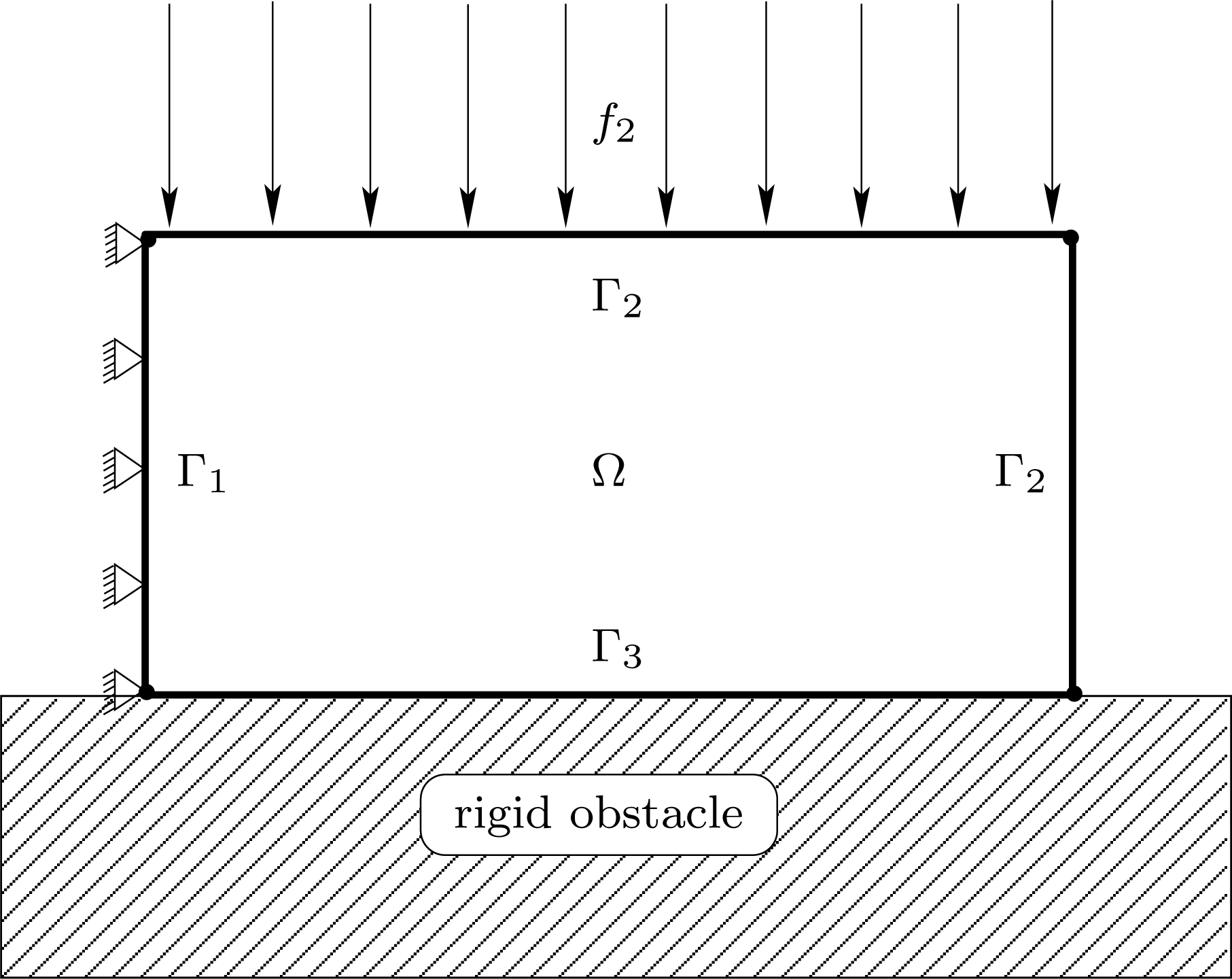
For the numerical simulation, let
 $\unicode[STIX]{x1D6FA}=(0,1)\times (0,0.5)$
with the metre as the length unit. The domain
 $\unicode[STIX]{x1D6FA}$
represents the cross-section of a three-dimensional linearly viscoelastic body subjected to the action of tractions in such a way that a plane stress hypothesis is valid. The physical setting of the contact problem is shown in Figure 9.1. On
 $\unicode[STIX]{x1D6E4}_{1}=\{0\}\times [0,0.5]$
the body is clamped, that is, the displacement field vanishes there. Let
 $\unicode[STIX]{x1D6E4}_{2}=((0,1)\times \{0.5\})\cup (\{1\}\times (0,0.5))$
; the part
 $(0,1)\times \{0.5\}$
is subject to vertical compressions and the part
 $\{1\}\times (0,0.5)$
is traction-free. No body forces are assumed to act on the elastic body during the process. On
 $\unicode[STIX]{x1D6E4}_{3}=(0,1)\times \{0\}$
, the body is in frictional bilateral contact with an obstacle. The friction follows the version (9.40) of Coulomb’s law, in which the friction bound depends on the tangential velocity
 $\Vert \dot{\boldsymbol{u}}_{\unicode[STIX]{x1D70F}}\Vert$
. For the coefficient of friction, we choose a function
 $\unicode[STIX]{x1D707}:[0,\infty )\rightarrow \mathbb{R}$
of the form
 $$\begin{eqnarray}\unicode[STIX]{x1D707}(r)=(a-b)\,\text{e}^{-\unicode[STIX]{x1D6FC}\,r}+b,\end{eqnarray}$$
with
 $a\geq b>0$
and
 $\unicode[STIX]{x1D6FC}>0$
. We take
 $a=1$
,
 $b=0.1$
and
 $\unicode[STIX]{x1D6FC}=200$
in the simulation. The friction law (9.40) with (9.47) describes the slip weakening phenomenon which appears in the study of geophysical problems; see Scholz (Reference Scholz1990) for details. The coefficient of friction decreases with the slip rate from the value
 $a$
to the limit value
 $b$
.
Numerical convergence orders.

The deformable material response is governed by a linearly viscoelastic constitutive law in which the viscosity tensor
 ${\mathcal{A}}$
and the elasticity tensor
 ${\mathcal{B}}$
are given by
 $$\begin{eqnarray}\displaystyle & & \displaystyle ({\mathcal{A}}\unicode[STIX]{x1D749})_{ij}=\unicode[STIX]{x1D707}_{1}(\unicode[STIX]{x1D70F}_{11}+\unicode[STIX]{x1D70F}_{22})\unicode[STIX]{x1D6FF}_{ij}+\unicode[STIX]{x1D707}_{2}\unicode[STIX]{x1D70F}_{ij},\quad 1\leq i,j\leq 2,\,\unicode[STIX]{x1D749}\in \mathbb{S}^{2},\nonumber\\ \displaystyle & & \displaystyle ({\mathcal{B}}\unicode[STIX]{x1D749})_{ij}=\displaystyle \frac{E\unicode[STIX]{x1D705}}{(1+\unicode[STIX]{x1D705})(1-2\unicode[STIX]{x1D705})}(\unicode[STIX]{x1D70F}_{11}+\unicode[STIX]{x1D70F}_{22})\unicode[STIX]{x1D6FF}_{ij}+\displaystyle \frac{E}{1+\unicode[STIX]{x1D705}}\unicode[STIX]{x1D70F}_{ij},\quad 1\leq i,j\leq 2,\,\unicode[STIX]{x1D749}\in \mathbb{S}^{2},\nonumber\end{eqnarray}$$
where
 $\unicode[STIX]{x1D707}_{1}$
and
 $\unicode[STIX]{x1D707}_{2}$
are viscosity constants,
 $E$
and
 $\unicode[STIX]{x1D705}$
are the Young’s modulus and Poisson ratio of the material and
 $\unicode[STIX]{x1D6FF}_{ij}$
denotes the Kronecker symbol. For the simulation, we use the values
 $\unicode[STIX]{x1D707}_{1}=50~\text{N}~\text{m}^{-2}$
,
 $\unicode[STIX]{x1D707}_{2}=100~\text{N}~\text{m}^{-2}$
,
 $E=2000~\text{N}~\text{m}^{-2}$
and
 $\unicode[STIX]{x1D705}=0.3$
. The mass density is chosen to be
 $\unicode[STIX]{x1D70C}=1000~\text{kg}~\text{m}^{-3}$
, and the force densities are
 $$\begin{eqnarray}\displaystyle \boldsymbol{f}_{0} & = & \displaystyle (0,-10^{-5})~\text{N}~\text{m}^{-2},\nonumber\\ \displaystyle \boldsymbol{f}_{2} & = & \displaystyle \left\{\begin{array}{@{}ll@{}}(0,0)~\text{N}~\text{m}^{-1}\quad & \text{on }\{1\}\times [0,0.5],\\ (0,-600\,t)~\text{N}~\text{m}^{-1}\quad & \text{on }[0,1]\times \{0.5\}.\end{array}\right.\nonumber\end{eqnarray}$$
For the initial values, we choose
 $$\begin{eqnarray}\boldsymbol{u}_{0}=\mathbf{0}~\text{m},\quad \boldsymbol{w}_{0}=\mathbf{0}~\text{m}~\text{s}^{-1}.\end{eqnarray}$$
Evolution of deformed meshes and frictional contact forces during the dynamic compression process.
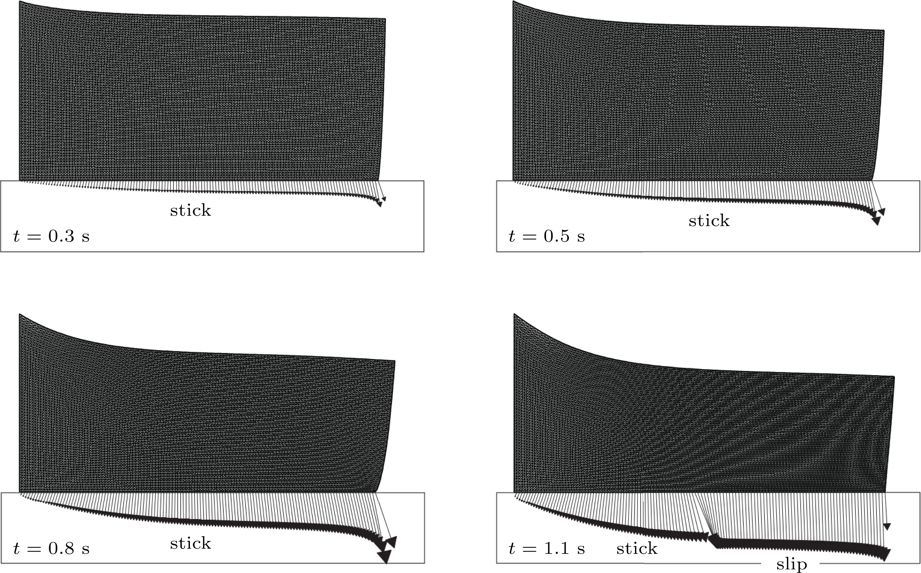
We compute a sequence of numerical solutions by using uniform triangulations of the domain
 $\unicode[STIX]{x1D6FA}$
and uniform partitions of the time interval
 $[0,1.1]$
(unit: second). We let
 $h$
denote the leg of a right triangle in a uniform triangulation and let
 $k$
be the time step-size. We start with
 $h=1/2$
and
 $k=1/2$
which are successively halved. The numerical solution corresponding to
 $h=1/256$
and
 $k=1/256$
is taken as the ‘exact’ solution and it is used to compute errors of the numerical solutions with larger
 $h$
and
 $k$
. The discrete problem corresponding to the fine triangulation with
 $h=1/256$
has
 $133\,896$
degrees of freedom at each time level. The numerical errors
 $\Vert \boldsymbol{u}-\boldsymbol{u}^{hk}\Vert _{V}$
are reported in Figure 9.2. A first-order convergence of
 $\Vert \boldsymbol{u}-\boldsymbol{u}^{hk}\Vert _{V}$
with respect to
 $h+k$
is clearly observed.
Finally, we provide some graphical results on the mechanical behaviour of the solution. Figure 9.3 shows the deformed configuration as well as the interface forces on
 $\unicode[STIX]{x1D6E4}_{3}$
during the dynamic compression process at times
 $t=0.3$
s,
 $t=0.5$
s,
 $t=0.8$
s and
 $t=1.1$
s. At the beginning of the process, the contact nodes are all in stick status. As the compression force becomes stronger, the friction bound is reached at more contact nodes where the status switches from stick to slip: see the graph at
 $t=1.1$
s.
10 Summary and outlook
Mathematical formulations of contact problems are naturally given in terms of inequalities. When the non-smooth and possibly multivalued constitutive relations and interface conditions are monotone, the contact problem has a convex structure and the mathematical formulation is in the form of a variational inequality. When the contact problem involves a non-monotone relation or condition, the mathematical formulation contains non-convex terms, and this leads to a hemivariational inequality which can be elliptic, history-dependent or evolutionary. The numerical solution of variational inequalities, in particular of those arising in contact mechanics, has been extensively studied in the literature. On the contrary, the numerical solution of hemivariational inequalities is still in an early stage, and many challenging issues remain to be addressed.
In this paper we have presented recent and new results on the numerical analysis of hemivariational inequalities arising in contact mechanics. We chose three representative contact problems to illustrate the main techniques used for the study of their numerical approximations and expected sample results. The three contact problems correspond to an elliptic, a history-dependent and an evolutionary hemivariational inequality, respectively. For the reader’s convenience, we tried to make the paper self-contained. We provide a concise review of basic knowledge from non-smooth analysis and include main steps of solution existence and uniqueness proofs of the hemivariational inequalities. The discrete analogues of the proofs can be used to show existence and uniqueness of numerical solutions. The temporal derivative was approximated by the backward divided difference and the integral in a history-dependent operator was approximated with the trapezoidal rule; other temporal approximations can be introduced and can be analysed similarly. For spatial discretizations, we used the finite element method. We derived optimal order error estimates for the linear element solutions with the previously mentioned temporal approximations under appropriate solution regularity assumptions. For the elliptic hemivariational inequality, we discussed convergence of the numerical solutions under basic solution regularity proved in the solution existence and uniqueness result. For the history-dependent and evolutionary hemivariational inequalities, it is also possible to prove convergence of the numerical solutions without assuming additional solution regularity. Owing to space limitations we have not provided such a convergence discussion in this paper, and instead refer the reader to Han and Reddy (Reference Han and Reddy1999, Reference Han and Reddy2000, Reference Han and Reddy2013), where convergence of numerical solutions is proved for evolutionary variational inequalities arising in elasto-plasticity under basic solution regularities available from solution existence and uniqueness results. Hemivariational inequalities arise in many other applications, and it is worth studying their numerical approximations as well; for example, Han, Huang, Wang and Xu (Reference Han, Huang, Wang and Xu2019) conduct numerical analysis on some hemivariational inequalities for applications related to semi-permeable media.
The results presented in this paper serve as a starting point in the development and analysis of more efficient numerical methods for solving hemivariational inequalities arising in contact mechanics. One promising research area is on a posteriori error analysis and adaptive mesh refinement for simulation of contact problems. Since the pioneering work of Babuška and Rheinboldt (Reference Babuška and Rheinboldt1978a , Reference Babuška and Rheinboldt1978b ), the field of a posteriori error analysis and adaptive algorithms for the numerical solution of differential equations has attracted many researchers, and a variety of different a posteriori error estimates have been proposed and analysed for mathematical models in various applications (see e.g. Ainsworth and Oden Reference Ainsworth and Oden2000, Babuška and Strouboulis Reference Babuška and Strouboulis2001, Verfürth Reference Verfürth2013). While a large percentage of the references in this area deal with boundary value problems of partial differential equations, one can also find papers on adaptive solution of variational inequalities arising in contact mechanics (e.g. Ben Belgacem, Bernardi, Blouza and Vohralík Reference Ben Belgacem, Bernardi, Blouza and Vohralík2012, Han Reference Han2005, Bostan and Han Reference Bostan, Han, Gao and Sherali2009, Hild and Lleras Reference Hild and Lleras2009). A natural step is to introduce a posteriori error estimators for hemivariational inequalities, analyse their reliability and efficiency, and use them to solve related contact problems.
Another research direction is to develop discontinuous Galerkin (DG) methods to solve hemivariational inequalities in contact mechanics. In DG methods, finite element functions of lower global smoothness are employed. The methods enjoy several advantages, such as handling easily general meshes with hanging nodes and elements of different shapes, accommodating easier parallel implementation Arnold, Brezzi, Cockburn and Marini (Reference Arnold, Brezzi, Cockburn and Marini2002), Cockburn, Karniadakis and Shu (Reference Cockburn, Karniadakis and Shu2000). DG methods have been successfully used to solve many different kind of mathematical problems. In particular, in the literature, one can find papers on DG methods for solving variational inequalities, including those arising in contact mechanics, for example Wang, Han and Cheng (Reference Wang, Han and Cheng2010, Reference Wang, Han and Cheng2011, Reference Wang, Han and Cheng2014) and Gudi and Porwal (Reference Gudi and Porwal2014, Reference Gudi and Porwal2016). However, DG methods have not been used to solve hemivariational inequalities and it will be interesting to explore the potential of the methods in larger-scale computer simulation of the contact problems.
Since the pioneering work of Beirão da Veiga et al. (Reference Beirão da Veiga, Brezzi, Cangiani, Manzini, Marini and Russo2013) and Alsaedi, Brezzi, Marini and Russo (Reference Alsaedi, Brezzi, Marini and Russo2013), virtual element methods (VEMs) have been used to solve a wide variety of PDE problems arising in solid mechanics, fluid mechanics and other areas of science and engineering. VEMs offer great flexibility in handling complex geometries. One key point is that the methods do not require explicit evaluation of the shape functions. Recently, VEMs have been used to solve variational inequalities. Wriggers, Rust and Reddy (Reference Wriggers, Rust and Reddy2016) simulated the problem of contact between two elastic bodies numerically using the VEM, though without theoretical analysis of the method. VEMs are used to solve an obstacle problem in Wang and Wei (Reference Wang and Wei2018a ), and to solve a simplified friction problem in Wang and Wei (Reference Wang and Wei2018b ); in both these papers, optimal order error estimates are derived. A general framework for VEMs is developed for solving elliptic variational inequalities of the second kind in Feng, Han and Huang (Reference Feng, Han and Huang2019); the methods discussed are directly implementable and optimal order error estimates are derived. It looks promising to develop VEMs to solve the contact problems, especially those more complicated ones in the form of hemivariational inequalities.
Acknowledgements
The present paper is a result of cooperation between the authors during the last five years. Part of the material included in this survey is related to our joint work with several collaborators, to whom we express our gratitude: M. Barboteu, K. Bartosz, Z. Huang, S. Migórski, A. Ochal, C. Wang, W. Xu, et al. We thank J. Sullian for helping us with some of the figures. We extend our thanks to the Editorial Board of Acta Numerica for inviting us to contribute to this issue. The work was supported by NSF under the grant DMS-1521684 and the European Union’s Horizon 2020 Research and Innovation Programme under the Marie Sklodowska-Curie Grant Agreement no. 823731 CONMECH.