1. Introduction
Numerical modelling of landslide-generated tsunamis in a complex fjord system is a challenging task. It can be achieved by coupling tsunami generation models, open-fjord propagation models and near-shore inundation models (Harbitz et al. Reference Harbitz, Glimsdal, Lovholt, Kveldsvik, Pedersen and Jensen2014). In the wave generation (source) region the interaction between the landslide and the water body is important and is extremely complex due to wave breaking, turbulence and air entrainment. The leading waves can be affected by frequency dispersion and the nonlinearity may also be considerable when the landslide speed is large. As waves propagate from the source region, wave amplitude decays as the consequence of directional spreading and increasing water depth. Hence, waves evolve into a regime where both frequency dispersion and nonlinearity are weak, but not negligible. The corresponding flow structures tend to become almost one-dimensional with wavefronts that are approximately perpendicular to the main axis of the fjord. Therefore, the main flow features maybe captured by a set of cross-sectionally averaged equations for weakly nonlinear and weakly dispersive waves. This flow regime is the focus of the present investigation.
Several one-dimensional theories of weakly nonlinear and weakly dispersive waves in a straight channel have been developed (Peregrine Reference Peregrine1968, Reference Peregrine1969; Shen Reference Shen1969; Fenton Reference Fenton1973; Shuto Reference Shuto1974; Miles Reference Miles1979; Chou Reference Chou1981; Kirby & Vengayil Reference Kirby and Vengayil1988; Teng Reference Teng1990, Reference Teng2000; Teng & Wu Reference Teng and Wu1992, Reference Teng and Wu1994, Reference Teng and Wu1997). It is also noted that in predicting flood flows in rivers, one-dimensional Saint-Venant models have been developed for channels with irregular geometries (e.g. Jacovkis & Tabak Reference Jacovkis and Tabak1996). However, none of these theories is able to account simultaneously for arbitrary cross-sections, appreciable changes of channel geometry within the wavelength scale in the direction of wave propagation and viscous boundary layer effects. The objective of this paper is then to present a long-wave model, which includes all the missing features mentioned above. The new model is intended to give insights to propagation of landslide-generated tsunamis in fjords, estuaries or channels. Specifically, it can be used as a tool to quickly forecast wave amplitudes and time of arrival of the leading waves at a coastal site.
Essentially the present model is an extension of the work developed by Teng & Wu (Reference Teng and Wu1992, Reference Teng and Wu1994, Reference Teng and Wu1997), referred as TW97 hereafter, to account for non-symmetric cross-sectional geometries where changes in the width and depth are important within the wavelength. The three-dimensional governing equations of motion for inviscid and incompressible fluid are first reduced to one-dimensional cross-sectional-averaged equations, describing the dominant wave motions along the longitudinal axis of the channel. The Boussinesq approximation is then used so that nonlinearity and frequency dispersion are relatively small, but of the same order of magnitude. Spanwise and vertical velocities are also assumed much smaller than the longitudinal velocity. Following Liu & Orfila’s (Reference Liu and Orfila2004) approach, the effects of the viscous boundary layer along the channel wall are included in the resulting governing equations. Its application is found to be adequate for laboratory-scale measurements. Channel curvature and branching are neglected in the present derivation. Although forcing caused by spatial gradients of the atmospheric pressure or a moving bottom can be easily included in the governing equations (see Teng & Wu Reference Teng and Wu1992), they are also not considered herein.
This paper is structured as follows. The following section introduces the basic governing equations and the scaling of the potential theory. In § 3, the cross-sectional-averaged equations for waves propagating in the longitudinal direction are obtained after invoking the Boussinesq approximation. Analytical expressions for the spanwise and vertical velocities, pressure and surface elevation on a cross-sectional plane are also proposed. In § 4, analytical and numerical examples for uniform channels, channels where the cross-sectional geometry changes slowly and channels where the depth and width variation is appreciable within the wavelength scale are presented. Numerical schemes developed to solve the Boussinesq-type equations for the longitudinal flow and boundary value problems at each cross-section are briefly discussed. Section 5 provides a discussion on the applicability and limitations of the present model.
2. Governing equations
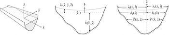
In this paper long-wave propagation in a straight channel with a non-uniform cross-section is considered. As depicted in figure 1, the channel cross-section is described by
 $\hat{z}=-{\hat{h}}(\hat{x},{\hat{y}})$
, where
 $\hat{z}$
is the vertical coordinate pointing upwards and
 $\hat{z}=0$
denotes the still water level (SWL). The
 $\hat{x}$
-axis is the longitudinal direction, while the
 ${\hat{y}}$
-axis represents the spanwise direction. The channel boundaries are rigid and impermeable. The channel cross-section geometry can alternatively be defined by
 ${\hat{y}}={\hat{y}}^{l}(\hat{x},\hat{z})$
and
 ${\hat{y}}=-{\hat{y}}^{r}(\hat{x},\hat{z})$
for the left and right channel bottom boundaries, measured from the channel axis (
 ${\hat{y}}=0$
). The intersections between the SWL and the channel boundary, describing the still water shorelines, are defined by
 $$\begin{eqnarray}{\hat{y}}={\hat{y}}^{l}(\hat{x},0)\equiv \hat{b}^{l}(\hat{x})\quad \text{and}\quad {\hat{y}}=-{\hat{y}}^{r}(\hat{x},0)\equiv -\hat{b}^{r}(\hat{x}),\end{eqnarray}$$
for the left and right sidewalls, respectively. The channel width below the SWL is therefore
 $$\begin{eqnarray}\hat{B}(\hat{x},\hat{z})={\hat{y}}^{l}(\hat{x},\hat{z})+{\hat{y}}^{r}(\hat{x},\hat{z}),\quad \text{on}~-{\hat{h}}\leqslant \hat{z}\leqslant 0,\end{eqnarray}$$
and
 $$\begin{eqnarray}\hat{B}_{0}(\hat{x})\equiv \hat{B}(\hat{x},0)=\hat{b}_{l}(\hat{x})+\hat{b}_{r}(\hat{x}),\quad \text{on}~\hat{z}=0,\end{eqnarray}$$
represents the surface width at the quiescent state. The instantaneous free-surface elevation is expressed as
 $\hat{z}=\hat{{\it\eta}}(\hat{x},{\hat{y}},\hat{t})$
, and the moving shorelines can be defined by
 $$\begin{eqnarray}{\hat{y}}={\hat{y}}^{l}(\hat{x},\hat{{\it\eta}}(t))\equiv {\hat{s}}^{l}(\hat{x},\hat{t})\quad \text{and}\quad {\hat{y}}=-{\hat{y}}^{r}(\hat{x},\hat{{\it\eta}}(t))\equiv -{\hat{s}}^{r}(\hat{x},\hat{t}),\end{eqnarray}$$
respectively.
Coordinate system and geometric parameters of the channel cross-section.

To describe the problem in terms of dimensionless variables, the characteristic wavelength
 $\hat{{\it\lambda}}$
is employed as the length scale in the longitudinal direction and the characteristic unperturbed water depth
 ${\hat{h}}_{0}$
as the length scale for the vertical direction. The length scale in the spanwise direction can be independent of the vertical length scale, i.e. water depth. However, it must be smaller than the water depth. Without loss of generality, the characteristic water depth
 ${\hat{h}}_{0}$
will also be used as the spanwise scale since cross-sectional averaging will be conducted in the following sections. This will avoid introducing another parameter in the analysis. The time scale is chosen as
 $\hat{{\it\lambda}}/{\hat{c}}_{0}$
, where
 ${\hat{c}}_{0}^{2}={\hat{g}}{\hat{h}}_{0}$
is the linear wave celerity in shallow water and
 ${\hat{g}}$
denotes the gravitational acceleration. Thus, the following dimensionless variables are introduced:
 $$\begin{eqnarray}x=\hat{x}/\hat{{\it\lambda}},\quad (y,z,h,b_{l},b_{r},s_{l},s_{r},B)=({\hat{y}},\hat{z},{\hat{h}},\hat{b}_{l},\hat{b}_{r},{\hat{s}}_{l},{\hat{s}}_{r},\hat{B})/{\hat{h}}_{0},\end{eqnarray}$$
 $$\begin{eqnarray}t=\hat{t}\left(\left.\sqrt{{\hat{g}}{\hat{h}}_{0}}\right/\hat{{\it\lambda}}\right).\end{eqnarray}$$
The velocity vector
 $\hat{\boldsymbol{u}}=(\hat{u} ,\hat{v},{\hat{w}})$
with components in the longitudinal, spanwise and vertical direction, respectively, is introduced. The dimensionless velocity components are expressed as
 $$\begin{eqnarray}u=\hat{u} \!\left/\!\left({\it\epsilon}\sqrt{{\hat{g}}{\hat{h}}_{0}}\right)\right.\quad \text{and}\quad (v,w)={\it\mu}(\hat{v},{\hat{w}})\!\left/\!\left({\it\epsilon}\sqrt{{\hat{g}}{\hat{h}}_{0}}\right)\right.,\end{eqnarray}$$
where two parameters,
 $$\begin{eqnarray}{\it\mu}={\hat{h}}_{0}/\hat{{\it\lambda}}\quad \text{and}\quad {\it\epsilon}=\hat{a}_{0}/{\hat{h}}_{0},\end{eqnarray}$$
representing the nonlinearity and frequency dispersion respectively, are introduced, in which
 $\hat{a}_{0}$
is the characteristic wave amplitude. The dimensionless surface elevation and pressure are
 $$\begin{eqnarray}{\it\eta}=\hat{{\it\eta}}/\hat{a}_{0}\quad \text{and}\quad p=\hat{p}/(\hat{{\it\rho}}{\hat{g}}\hat{a}_{0}),\end{eqnarray}$$
where
 $\hat{{\it\rho}}$
represents the density of water.
Assuming that water is incompressible and ignoring the viscous effects, the governing equations for wave motions can be written in dimensionless form as
 $$\begin{eqnarray}\frac{\partial u}{\partial x}+\frac{1}{{\it\mu}^{2}}\left(\frac{\partial v}{\partial y}+\frac{\partial w}{\partial z}\right)=0,\end{eqnarray}$$
for the mass conservation, and
 $$\begin{eqnarray}\displaystyle & \displaystyle \frac{\partial u}{\partial t}+{\it\epsilon}\left[\frac{\partial }{\partial x}(u^{2})+\frac{1}{{\it\mu}^{2}}\left\{\frac{\partial }{\partial y}(uv)+\frac{\partial }{\partial z}(uw)\right\}\right]=-\frac{\partial p}{\partial x}, & \displaystyle\end{eqnarray}$$
 $$\begin{eqnarray}\displaystyle & \displaystyle \frac{\partial v}{\partial t}+{\it\epsilon}\left[\frac{\partial }{\partial x}(uv)+\frac{1}{{\it\mu}^{2}}\left\{\frac{\partial }{\partial y}(v^{2})+\frac{\partial }{\partial z}(vw)\right\}\right]=-\frac{\partial p}{\partial y}, & \displaystyle\end{eqnarray}$$
 $$\begin{eqnarray}\displaystyle & \displaystyle \frac{\partial w}{\partial t}+{\it\epsilon}\left[\frac{\partial }{\partial x}(uw)+\frac{1}{{\it\mu}^{2}}\left\{\frac{\partial }{\partial y}(vw)+\frac{\partial }{\partial z}(w^{2})\right\}\right]=-\frac{\partial p}{\partial z}-\frac{1}{{\it\epsilon}}, & \displaystyle\end{eqnarray}$$
 $\boldsymbol{{\rm\nabla}}\times \boldsymbol{u}=0$
, thus a velocity potential,
 $\boldsymbol{{\rm\nabla}}{\it\phi}=\boldsymbol{u}$
, can be introduced, where
 $\boldsymbol{u}=(u,v,w)$
. The conservation of energy can be expressed by means of the Bernoulli equation
 $$\begin{eqnarray}\frac{\partial {\it\phi}}{\partial t}+\frac{1}{2}{\it\epsilon}\left[u^{2}+\frac{1}{{\it\mu}^{2}}(v^{2}+w^{2})\right]+p+\frac{z}{{\it\epsilon}}=0,\end{eqnarray}$$
where the Bernoulli constant has been absorbed into the velocity potential. The kinematic boundary condition on the free surface is expressed as
 $$\begin{eqnarray}w={\it\mu}^{2}\left(\frac{\partial {\it\eta}}{\partial t}+{\it\epsilon}u\frac{\partial {\it\eta}}{\partial x}\right)+{\it\epsilon}v\frac{\partial {\it\eta}}{\partial y},\quad \text{on}~z={\it\epsilon}{\it\eta}(x,y,t).\end{eqnarray}$$
The no-flux boundary condition along the bottom requires
 $$\begin{eqnarray}w=-{\it\mu}^{2}u\frac{\partial h}{\partial x}-v\frac{\partial h}{\partial y},\quad \text{on}~z=-h(x,y).\end{eqnarray}$$
Along the moving shorelines on the channel banks, the kinematic boundary conditions are
 $$\begin{eqnarray}{\it\epsilon}v={\it\mu}^{2}\left(\frac{\partial s_{l}}{\partial t}+{\it\epsilon}u\frac{\partial s_{l}}{\partial x}\right),\quad \text{on}~y=s_{l}(x,t)\end{eqnarray}$$
and
 $$\begin{eqnarray}{\it\epsilon}v=-{\it\mu}^{2}\left(\frac{\partial s_{r}}{\partial t}+{\it\epsilon}u\frac{\partial s_{r}}{\partial x}\right),\quad \text{on}~y=-s_{r}(x,t),\end{eqnarray}$$
for the left and right sidewalls, respectively. Finally the atmospheric pressure variation on the free surface is ignored. Thus,
 $$\begin{eqnarray}p=0,\quad \text{on}~z={\it\epsilon}{\it\eta}(x,y,t).\end{eqnarray}$$
Equations (2.9) to (2.18) constitute the governing equations and boundary conditions for a general three-dimensional nonlinear water wave problem without considering viscous effects. Additional initial conditions for free-surface elevation and velocity, and upstream and downstream boundary conditions are needed for a specific problem of interest. A wave propagation model expressed in terms of cross-sectional-averaged longitudinal velocity and spanwise-averaged free-surface elevation will be derived in the following section. Viscous effects will be considered in § 4.4 via boundary layer flow analyses.
3. Cross-sectional-averaged wave equations
The flow problem stated in the previous section can be reduced to a set of one-dimensional governing equations by averaging over a channel cross-section and applying the boundary conditions on the free surface and solid boundaries. The cross-sectional area at the quiescent state
 $A_{0}(x)$
and the instantaneous cross-sectional area
 $A(x,t)$
are defined by
 $$\begin{eqnarray}A_{0}(x)=\int _{-b_{r}}^{b_{l}}h(x,y)\text{d}y=\int _{-max(h)}^{0}B(x,z)\text{d}z\end{eqnarray}$$
and
 $$\begin{eqnarray}A(x,t)=A_{0}+\int _{-s_{r}}^{-b_{r}}({\it\epsilon}{\it\eta}-h)\text{d}y+{\it\epsilon}\int _{-b_{r}}^{b_{l}}{\it\eta}\text{d}y+\int _{b_{l}}^{s_{l}}({\it\epsilon}{\it\eta}-h)\text{d}y,\end{eqnarray}$$
respectively. The cross-sectional average of a function
 $f(x,y,z,t)$
is defined as
 $$\begin{eqnarray}\langle \,f\rangle =\frac{1}{A}\int _{-s_{r}}^{s_{l}}\int _{-h}^{{\it\epsilon}{\it\eta}}f(x,y,z,t)\text{d}z\text{d}y.\end{eqnarray}$$
Although the averaging process of the governing equations is straightforward, some of the details are presented in appendix A for completeness. The resulting cross-sectional-averaged equations of motions are
 $$\begin{eqnarray}\frac{1}{{\it\epsilon}}\frac{\partial A}{\partial t}+\frac{\partial (\langle u\rangle A)}{\partial x}=0\end{eqnarray}$$
and
 $$\begin{eqnarray}\frac{\partial }{\partial t}(A\langle u\rangle )+{\it\epsilon}\frac{\partial }{\partial x}(A\langle uu\rangle )=-A\left\langle \frac{\partial p}{\partial x}\right\rangle ,\end{eqnarray}$$
for the conservation of mass and momentum, respectively. Equations (3.4) and (3.5) are exact for a channel of arbitrary cross-section; no restriction has been imposed on the parameters,
 ${\it\epsilon}$
and
 ${\it\mu}$
. A similar set of equations was derived in dimensional form by Teng & Wu (Reference Teng and Wu1992, equations (12) and (13)). In their derivation, the geometry of the cross-section was required to be symmetric with respect to the centreline of the channel. It is shown in the appendix A that this requirement is unnecessary.
For later use, two additional cross-sectional-averaged quantities of a function
 $f(x,y,z,t)$
are introduced:
 $$\begin{eqnarray}\overline{f}=\frac{1}{A_{0}}\int _{-b_{r}}^{b_{l}}\int _{-h}^{0}f(x,y,z,t)\text{d}z\text{d}y\end{eqnarray}$$
and
 $$\begin{eqnarray}\widetilde{f|_{z=0}}=\frac{1}{B_{0}}\int _{-b_{r}}^{b_{l}}f(x,y,0,t)\text{d}y.\end{eqnarray}$$
Equation (3.6) can be interpreted as the averaged value over the channel cross-sectional area at the quiescent state, while (3.7) denotes the averaged value over the channel still water surface width.
3.1. Boussinesq approximation
In (3.4) and (3.5),
 $\langle uu\rangle$
and
 $\langle \partial p/\partial x\rangle$
need to be further related to the cross-sectional-averaged velocity
 $\langle u\rangle$
and surface-width-averaged free-surface elevation
 $\widetilde{{\it\eta}}$
. To accomplish this, additional approximations are needed. First of all, the Boussinesq approximation is invoked, i.e.
 $O({\it\epsilon})=O({\it\mu}^{2})\ll O(1)$
; therefore, the theory is applicable only for weakly nonlinear and weakly dispersive waves. A second step is to expand the dimensionless physical variables as power series of
 ${\it\mu}^{2}$
:
 $$\begin{eqnarray}\displaystyle & {\it\phi}={\it\phi}_{1}(x,t)+{\it\mu}^{2}{\it\phi}_{2}(x,y,z,t)+O({\it\mu}^{4}), & \displaystyle\end{eqnarray}$$
 $$\begin{eqnarray}\displaystyle & {\it\eta}={\it\eta}_{1}(x,t)+{\it\mu}^{2}{\it\eta}_{2}(x,y,t)+O({\it\mu}^{4}), & \displaystyle\end{eqnarray}$$
 $$\begin{eqnarray}\displaystyle & u=u_{1}(x,t)+{\it\mu}^{2}u_{2}(x,y,z,t)+O({\it\mu}^{4}), & \displaystyle\end{eqnarray}$$
 $$\begin{eqnarray}\displaystyle & v={\it\mu}^{2}v_{2}(x,y,z,t)+O({\it\mu}^{4}), & \displaystyle\end{eqnarray}$$
 $$\begin{eqnarray}\displaystyle & w={\it\mu}^{2}w_{2}(x,y,z,t)+O({\it\mu}^{4}). & \displaystyle\end{eqnarray}$$
 $O(v)=O(w)\ll O(u)$
. We remark here that if the channel width is scaled differently from the water depth, the spanwise velocity will be much weaker than the vertical velocity when the channel width is smaller than the water depth. With these power series expansions, it is shown in appendix B that
 $$\begin{eqnarray}\langle uu\rangle =\langle u\rangle \langle u\rangle +O({\it\mu}^{4})\end{eqnarray}$$
and
 $$\begin{eqnarray}\left\langle \frac{\partial p}{\partial x}\right\rangle =\frac{\partial \widetilde{{\it\eta}}}{\partial x}+{\it\mu}^{2}\left[\frac{\partial }{\partial x}\left(\widetilde{\left.\frac{\partial {\it\phi}_{2}}{\partial t}\right|_{z=0}}\right)-\overline{\frac{\partial ^{2}{\it\phi}_{2}}{\partial x\partial t}}\right]+O({\it\epsilon}{\it\mu}^{2},{\it\mu}^{4}).\end{eqnarray}$$
As shown in appendix C, the instantaneous cross-sectional area
 $A(x,t)$
is expressed as
 $$\begin{eqnarray}A=A_{0}+{\it\epsilon}B_{0}\widetilde{{\it\eta}}+{\it\epsilon}^{2}\frac{B_{0}^{\prime }}{2}\widetilde{{\it\eta}}^{2}+O({\it\epsilon}^{2}{\it\mu}^{2},{\it\epsilon}^{3}),\end{eqnarray}$$
in which
 $$\begin{eqnarray}B_{0}^{\prime }(x)\equiv \frac{\partial B}{\partial z}(x,0).\end{eqnarray}$$
For channels with the sidewall slope being
 $O(1)$
, the instantaneous cross-section average
 $\langle \,f\rangle$
and the cross-sectional average at the quiescent state
 $\overline{f}$
are related as follows:
 $$\begin{eqnarray}\langle \,f\rangle =\overline{f}+O({\it\epsilon}).\end{eqnarray}$$
Substituting (3.15) into the continuity equation (3.4) yields
 $$\begin{eqnarray}\frac{\partial \widetilde{{\it\eta}}}{\partial t}+{\it\epsilon}\frac{B_{0}^{\prime }}{2B_{0}}\frac{\partial \widetilde{{\it\eta}}^{2}}{\partial t}+\frac{1}{B_{0}}\frac{\partial }{\partial x}\left[\langle u\rangle (A_{0}+{\it\epsilon}B_{0}\widetilde{{\it\eta}})\right]=O({\it\epsilon}^{2},{\it\epsilon}{\it\mu}^{2},{\it\mu}^{4}).\end{eqnarray}$$
The second term in the equation above can be manipulated by replacing the time derivative of
 $\widetilde{{\it\eta}}$
with a spatial derivative obtained from the leading-order terms of the same equation. Thus,
 $$\begin{eqnarray}\frac{\partial \widetilde{{\it\eta}}}{\partial t}+\frac{1}{B_{0}}\frac{\partial }{\partial x}[\langle u\rangle A_{0}]-{\it\epsilon}\frac{B_{0}^{\prime }}{B_{0}^{2}}\widetilde{{\it\eta}}\frac{\partial }{\partial x}[\langle u\rangle A_{0}]+\frac{{\it\epsilon}}{B_{0}}\frac{\partial }{\partial x}[\langle u\rangle B_{0}\widetilde{{\it\eta}}]=O({\it\epsilon}^{2},{\it\epsilon}{\it\mu}^{2},{\it\mu}^{4}).\end{eqnarray}$$
Similarly, substituting (3.13), (3.14) and (3.15) into the momentum equation (3.5), after some manipulations, yields
 $$\begin{eqnarray}\frac{\partial \langle u\rangle }{\partial t}+\frac{\partial \widetilde{{\it\eta}}}{\partial x}+{\it\epsilon}\langle u\rangle \frac{\partial \langle u\rangle }{\partial x}+{\it\mu}^{2}\mathfrak{D}=O({\it\epsilon}^{2},{\it\epsilon}{\it\mu}^{2},{\it\mu}^{4}),\end{eqnarray}$$
where
 $$\begin{eqnarray}\mathfrak{D}(x,t)=\frac{\partial }{\partial x}\left(\widetilde{\left.\frac{\partial {\it\phi}_{2}}{\partial t}\right|_{z=0}}\right)-\overline{\frac{\partial ^{2}{\it\phi}_{2}}{\partial x\partial t}}.\end{eqnarray}$$
Equations (3.19) and (3.20) are the governing equations for
 $\langle u\rangle$
and
 $\widetilde{{\it\eta}}$
. However,
 $\mathfrak{D}$
or
 ${\it\phi}_{2}$
needs to be described.
3.2. Velocity, surface elevation and pressure on a cross-sectional plane
On a channel cross-section, the governing equation for
 ${\it\phi}_{2}$
can be derived by substituting the perturbation expansions, (3.8)–(3.12), into the conservation of mass, (2.9) and taking the cross-sectional average of the resulting equation. This yields
 $$\begin{eqnarray}\frac{\partial ^{2}{\it\phi}_{2}}{\partial y^{2}}+\frac{\partial ^{2}{\it\phi}_{2}}{\partial z^{2}}=-\frac{\partial \langle u\rangle }{\partial x},\quad \text{on}~-h(x,y)<z<0.\end{eqnarray}$$
Using the leading-order term of (3.19) in the linearized free-surface boundary condition (2.14) yields
 $$\begin{eqnarray}\frac{\partial {\it\phi}_{2}}{\partial z}=-\frac{A_{0}}{B_{0}}\frac{\partial \langle u\rangle }{\partial x}-\frac{1}{B_{0}}\frac{\text{d}A_{0}}{\text{d}x}\langle u\rangle ,\quad \text{on}\;z=0.\end{eqnarray}$$
The no-flux boundary condition along the channel bottom (2.15) requires
 $$\begin{eqnarray}\frac{\partial {\it\phi}_{2}}{\partial n}=-\frac{\displaystyle \langle u\rangle \frac{\partial h}{\partial x}}{\sqrt{\displaystyle \left(\frac{\partial h}{\partial y}\right)^{2}+1}},\quad \text{on}~z=-h(x,y),\end{eqnarray}$$
in which
 $n$
denotes the unit normal (in the
 $y$
–
 $z$
plane) along the channel bottom at a fixed
 $x$
. The leading-order error of the boundary value problem for
 ${\it\phi}_{2}$
, (3.22)–(3.24), is of
 $O({\it\epsilon},{\it\mu}^{2})$
and is consistent with that of the momentum equation (3.20), where
 $\mathfrak{D}$
is multiplied by
 ${\it\mu}^{2}$
. If the channel is bounded by vertical walls, two additional boundary conditions are required:
 $$\begin{eqnarray}\frac{\partial {\it\phi}_{2}}{\partial y}=\langle u\rangle \left(-\frac{\text{d}b_{l}}{\text{d}x},\frac{\text{d}b_{r}}{\text{d}x}\right)+O({\it\mu}^{2}),\quad \text{on}~y=b_{l}(x),-b_{r}(x).\end{eqnarray}$$
Since the boundary value problem for
 ${\it\phi}_{2}$
is linear and is only forced by
 $\langle u\rangle$
and
 $\partial \langle u\rangle /\partial x$
, the following solution form is sought:
 $$\begin{eqnarray}{\it\phi}_{2}(x,y,z,t)={\it\chi}_{1}(x,y,z)\langle u\rangle +{\it\chi}_{2}(x,y,z)\frac{\partial \langle u\rangle }{\partial x}+F(x,t),\end{eqnarray}$$
in which
 $F(x,t)$
is an arbitrary function and does not contribute to the velocity field (see (3.20) and (3.21)). Substituting (3.26) into (3.22)–(3.24), the boundary value problems for
 ${\it\chi}_{1}$
and
 ${\it\chi}_{2}$
can be expressed as
 $$\begin{eqnarray}\displaystyle & \displaystyle \frac{\partial ^{2}{\it\chi}_{1}}{\partial y^{2}}+\frac{\partial ^{2}{\it\chi}_{1}}{\partial z^{2}}=0,\quad \text{on}\;-h(x,y)<z<0, & \displaystyle\end{eqnarray}$$
 $$\begin{eqnarray}\displaystyle & \displaystyle \frac{\partial {\it\chi}_{1}}{\partial z}=-\frac{1}{B_{0}}\frac{\text{d}A_{0}}{\text{d}x},\quad \text{on}\;z=0, & \displaystyle\end{eqnarray}$$
 $$\begin{eqnarray}\displaystyle & \displaystyle \frac{\partial {\it\chi}_{1}}{\partial n}=-\frac{\displaystyle \frac{\partial h}{\partial x}}{\sqrt{\displaystyle \left(\frac{\partial h}{\partial y}\right)^{2}+1}},\quad \text{on}\;z=-h(x,y) & \displaystyle\end{eqnarray}$$
 $$\begin{eqnarray}\displaystyle & \displaystyle \frac{\partial ^{2}{\it\chi}_{2}}{\partial y^{2}}+\frac{\partial ^{2}{\it\chi}_{2}}{\partial z^{2}}=-1,\quad \text{on}\;-h(x,y)<z<0, & \displaystyle\end{eqnarray}$$
 $$\begin{eqnarray}\displaystyle & \displaystyle \frac{\partial {\it\chi}_{2}}{\partial z}=-\frac{A_{0}}{B_{0}},\quad \text{on}\;z=0, & \displaystyle\end{eqnarray}$$
 $$\begin{eqnarray}\displaystyle & \displaystyle \frac{\partial {\it\chi}_{2}}{\partial n}=0,\quad \text{on}\;z=-h(x,y). & \displaystyle\end{eqnarray}$$
 ${\it\chi}_{1}$
and
 ${\it\chi}_{2}$
need to be invoked:
 $$\begin{eqnarray}\frac{\partial {\it\chi}_{1}}{\partial y}=\left(-\frac{\text{d}b_{l}}{\text{d}x},\frac{\text{d}b_{r}}{\text{d}x}\right)\quad \text{and}\quad \frac{\partial {\it\chi}_{2}}{\partial y}=0,\quad \text{on}\;y=b_{l}(x),-b_{r}(x).\end{eqnarray}$$
The function
 ${\it\chi}_{1}$
is a new contribution of the present theory, representing the effects of changes of cross-sectional geometry in the direction of wave propagation which are appreciable within a wavelength. These effects were not considered in Peregrine (Reference Peregrine1968) and TW97. Functions
 ${\it\chi}_{1}$
and
 ${\it\chi}_{2}$
depend only on the geometry of the channel and can be calculated either numerically or analytically, once the channel configuration is prescribed. Several numerical methods, i.e. finite differences, finite elements and boundary elements, can be used to solve the boundary value problems for
 ${\it\chi}_{1}$
and
 ${\it\chi}_{2}$
. Analytical solutions can also be obtained for simple geometries such as rectangular and triangular cross-sections.
Three-dimensional features of the velocity field as well as the pressure field can be recovered from the perturbation solutions once the cross-sectional-averaged quantities
 $\langle u\rangle (x,t)$
,
 $\widetilde{{\it\eta}}(x,t)$
, together with the functions
 ${\it\chi}_{1}(x,y,z)$
and
 ${\it\chi}_{2}(x,y,z)$
, are computed. The expressions for the velocity components, with a leading-order error of
 $O({\it\epsilon}^{2},{\it\epsilon}{\it\mu}^{2},{\it\mu}^{4})$
, are
 $$\begin{eqnarray}\displaystyle & \displaystyle u(x,y,z,t)=\langle u\rangle +{\it\mu}^{2}({\it\chi}_{1}-\overline{{\it\chi}_{1}})\frac{\partial \langle u\rangle }{\partial x}+{\it\mu}^{2}({\it\chi}_{2}-\overline{{\it\chi}_{2}})\frac{\partial ^{2}\langle u\rangle }{\partial x^{2}}, & \displaystyle\end{eqnarray}$$
 $$\begin{eqnarray}\displaystyle & \displaystyle v(x,y,z,t)={\it\mu}^{2}\left(\frac{\partial {\it\chi}_{1}}{\partial y}\langle u\rangle +\frac{\partial {\it\chi}_{2}}{\partial y}\frac{\partial \langle u\rangle }{\partial x}\right), & \displaystyle\end{eqnarray}$$
 $$\begin{eqnarray}\displaystyle & \displaystyle w(x,y,z,t)={\it\mu}^{2}\left(\frac{\partial {\it\chi}_{1}}{\partial z}\langle u\rangle +\frac{\partial {\it\chi}_{2}}{\partial z}\frac{\partial \langle u\rangle }{\partial x}\right). & \displaystyle\end{eqnarray}$$
 $$\begin{eqnarray}{\it\eta}(x,y,t)=\widetilde{{\it\eta}}+{\it\mu}^{2}\left(\widetilde{\left.{\it\chi}_{1}\right|_{z=0}}-\left.{\it\chi}_{1}\right|_{z=0}\right)\frac{\partial \langle u\rangle }{\partial t}+{\it\mu}^{2}\left(\widetilde{\left.{\it\chi}_{2}\right|_{z=0}}-\left.{\it\chi}_{2}\right|_{z=0}\right)\frac{\partial ^{2}\langle u\rangle }{\partial t\partial x},\end{eqnarray}$$
and the pressure becomes
 $$\begin{eqnarray}p(x,y,z,t)=\widetilde{{\it\eta}}+{\it\mu}^{2}\left(\widetilde{\left.{\it\chi}_{1}\right|_{z=0}}-{\it\chi}_{1}\right)\frac{\partial \langle u\rangle }{\partial t}+{\it\mu}^{2}\left(\widetilde{\left.{\it\chi}_{2}\right|_{z=0}}-{\it\chi}_{2}\right)\frac{\partial ^{2}\langle u\rangle }{\partial t\partial x}-\frac{z}{{\it\epsilon}}.\end{eqnarray}$$
Examples of the velocity field and surface elevation are given in § 4.1 for simple geometries.
3.3. One-dimensional cross-sectional-averaged Boussinesq equations
Once
 ${\it\chi}_{1}$
and
 ${\it\chi}_{2}$
are calculated for a given channel geometry, (3.26) can be substituted into (3.21) to get
 $$\begin{eqnarray}\mathfrak{D}(x,t)={\it\alpha}\frac{\partial \langle u\rangle }{\partial t}+{\it\beta}\frac{\partial ^{2}\langle u\rangle }{\partial t\partial x}+{\it\gamma}\frac{\partial ^{3}\langle u\rangle }{\partial t\partial x^{2}},\end{eqnarray}$$
where
 $$\begin{eqnarray}\displaystyle & \displaystyle {\it\alpha}(x)=\frac{\partial }{\partial x}\left[\widetilde{\left.{\it\chi}_{1}\right|_{z=0}}\right]-\overline{\frac{\partial {\it\chi}_{1}}{\partial x}}, & \displaystyle\end{eqnarray}$$
 $$\begin{eqnarray}\displaystyle & \displaystyle {\it\beta}(x)=\widetilde{\left.{\it\chi}_{1}\right|_{z=0}}-\overline{{\it\chi}_{1}}+\frac{\partial }{\partial x}\left[\widetilde{\left.{\it\chi}_{2}\right|_{z=0}}\right]-\overline{\frac{\partial {\it\chi}_{2}}{\partial x}}, & \displaystyle\end{eqnarray}$$
 $$\begin{eqnarray}\displaystyle & \displaystyle {\it\gamma}(x)=\widetilde{\left.{\it\chi}_{2}\right|_{z=0}}-\overline{{\it\chi}_{2}} & \displaystyle\end{eqnarray}$$
 ${\it\alpha},{\it\beta}=0$
. Finally the momentum equation (3.20) can be rewritten in the following form:
 $$\begin{eqnarray}(1+{\it\mu}^{2}{\it\alpha})\frac{\partial \langle u\rangle }{\partial t}+\frac{\partial \widetilde{{\it\eta}}}{\partial x}+{\it\epsilon}\langle u\rangle \frac{\partial \langle u\rangle }{\partial x}+{\it\mu}^{2}{\it\beta}\frac{\partial ^{2}\langle u\rangle }{\partial t\partial x}+{\it\mu}^{2}{\it\gamma}\frac{\partial ^{3}\langle u\rangle }{\partial t\partial x^{2}}=O({\it\epsilon}^{2},{\it\epsilon}{\it\mu}^{2},{\it\mu}^{4}).\end{eqnarray}$$
Equations (3.19) and (3.43) are the governing equations for the cross-sectional-averaged longitudinal velocity,
 $\langle u\rangle$
, and the spanwise-averaged free-surface elevation,
 $\widetilde{{\it\eta}}$
. Properly described initial conditions and upstream/downstream boundary conditions in the channel are needed to solve the initial boundary value problem. Since the Boussinesq approximation has been employed, the governing equations are suitable for modelling weakly nonlinear and weakly dispersive waves. The coefficients
 ${\it\alpha},{\it\beta}$
and
 ${\it\gamma}$
in these equations depend only on the cross-sectional geometry, which is allowed to vary significantly within a wavelength. Specifically, the term associated with
 ${\it\alpha}$
represents the correction to the local acceleration, whereas the term associated with
 ${\it\beta}$
denotes the wave decay or amplification caused by the variation of the cross-sectional geometry along the channel. Both terms are negligible when the channel variations in the longitudinal direction become very small. The term associated with
 ${\it\gamma}$
represents the frequency dispersion effects, which remain important even when the channel variations in the longitudinal direction are small. Finally, for a straight rectangular channel, (3.19) and (3.43) reduce to the one-dimensional version of the original Boussinesq equation exactly (Peregrine Reference Peregrine1967).
3.4. Analytical expressions for
 ${\it\chi}_{1}(x,y,z)$
and
${\it\chi}_{2}(x,y,z)$


In this section, analytical solutions of
 ${\it\chi}_{1}$
and
 ${\it\chi}_{2}$
for rectangular and triangular cross-sections are presented. The corresponding coefficients
 ${\it\alpha},{\it\beta}$
and
 ${\it\gamma}$
can also be expressed analytically. For an arbitrary cross-section geometry,
 ${\it\chi}_{1}$
and
 ${\it\chi}_{2}$
need to be obtained numerically, as will be presented in § 4.1.
3.4.1. Rectangular channel
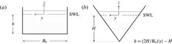
Figure 2(a) depicts a rectangular channel of width
 $B_{0}$
, depth
 $h$
and boundaries located at
 $y=B_{0}/2$
, and
 $-B_{0}/2$
. For this configuration, functions
 ${\it\chi}_{1}$
and
 ${\it\chi}_{2}$
are
 $$\begin{eqnarray}\displaystyle & \displaystyle {\it\chi}_{1}(x,y,z)=\frac{1}{2B_{0}}\frac{\text{d}B_{0}}{\text{d}x}\left[-2hz-z^{2}+y^{2}\right]-\frac{\text{d}h}{\text{d}x}z, & \displaystyle\end{eqnarray}$$
 $$\begin{eqnarray}\displaystyle & \displaystyle {\it\chi}_{2}(x,y,z)=-hz-\frac{z^{2}}{2}. & \displaystyle\end{eqnarray}$$
 $$\begin{eqnarray}\displaystyle & \displaystyle {\it\alpha}=-\frac{h^{2}}{3B_{0}}\frac{\text{d}^{2}B_{0}}{\text{d}x^{2}}+\left(\frac{1}{12}+\frac{h^{2}}{3B_{0}^{2}}\right)\left(\frac{\text{d}B_{0}}{\text{d}x}\right)^{2}-\frac{h}{2B_{0}}\frac{\text{d}h}{\text{d}x}\frac{\text{d}B_{0}}{\text{d}x}-\frac{h}{2}\frac{\partial ^{2}h}{\partial x^{2}}, & \displaystyle\end{eqnarray}$$
 $$\begin{eqnarray}\displaystyle & \displaystyle {\it\beta}=-h\left(\frac{h}{3B_{0}}\frac{\text{d}B_{0}}{\text{d}x}+\frac{\text{d}h}{\text{d}x}\right), & \displaystyle\end{eqnarray}$$
 $$\begin{eqnarray}\displaystyle & \displaystyle {\it\gamma}=-\frac{h^{2}}{3}. & \displaystyle\end{eqnarray}$$
 ${\it\alpha}$
and
 ${\it\beta}$
depend on the rate of change in channel width and depth along the direction of wave propagation, whereas
 ${\it\gamma}$
depends only on the local depth. For the case where the channel has a constant width, i.e.
 $B_{0}=$
constant, the above coefficients reduce to
 $$\begin{eqnarray}{\it\alpha}=-\frac{h}{2}\frac{\text{d}^{2}h}{\text{d}x^{2}},\quad {\it\beta}=-h\frac{\text{d}h}{\text{d}x},\quad {\it\gamma}=-\frac{h^{2}}{3},\end{eqnarray}$$
so the contribution of the terms associated with
 ${\it\alpha}$
and
 ${\it\beta}$
depend on changes in the water depth along the channel. Using the above coefficients in (3.43), the original one-dimensional version of the Boussinesq equation by Peregrine (Reference Peregrine1967) is recovered, in which the percentage change of water depth within a wavelength is allowed to be of order-one. Section 4.4.1 includes the analysis of solitary waves propagating over a channel of constant width and uniform slope (Liu et al.
Reference Liu, Simarro, Vandever and Orfila2006), where expressions (3.49) apply. For the case where the water depth remains a constant while the channel width varies, the coefficients become
 $$\begin{eqnarray}{\it\alpha}=\left(\frac{1}{12}+\frac{h^{2}}{3B_{0}^{2}}\right)\left(\frac{\text{d}B_{0}}{\text{d}x}\right)^{2},\quad {\it\beta}=-\frac{h^{2}}{3B_{0}}\frac{\text{d}B_{0}}{\text{d}x},\quad {\it\gamma}=-\frac{h^{2}}{3}.\end{eqnarray}$$
Various examples for waves propagating in convergent and divergent channels of constant depth, where (3.50) apply, are analysed in § 4. For uniform channels, the coefficients in the governing equations become
 $$\begin{eqnarray}{\it\alpha}={\it\beta}=0,\quad {\it\gamma}=-\frac{h^{2}}{3}.\end{eqnarray}$$
Note that for a rectangular channel,
 ${\it\gamma}$
is always negative. Waves propagating along uniform channels are analysed in § 4.1.
Definitions for (a) rectangular and (b) triangular cross-sections.

3.4.2. Triangular channel
For a channel with a symmetric triangular cross-section (figure 2 b), the channel boundary can be expressed as
 $$\begin{eqnarray}z=-h(x,y)=\frac{2H}{B_{0}}|y|-H,\end{eqnarray}$$
where
 $B_{0}$
is the surface width and
 $H$
denotes the maximum depth along the centreline (figure 2
b). The analytical solutions for
 ${\it\chi}_{1}$
and
 ${\it\chi}_{2}$
can be obtained as
 $$\begin{eqnarray}{\it\chi}_{1}=-\frac{1}{2}\left(\frac{H}{B_{0}}\frac{\text{d}B_{0}}{\text{d}x}+\frac{\text{d}H}{\text{d}x}\right)z+\left(\frac{1}{4H}\frac{\text{d}H}{\text{d}x}-\frac{1}{4B_{0}}\frac{\text{d}B_{0}}{\text{d}x}\right)(z^{2}-y^{2}),\end{eqnarray}$$
and
 $$\begin{eqnarray}{\it\chi}_{2}=-{\textstyle \frac{1}{4}}(2Hz+z^{2}+y^{2}).\end{eqnarray}$$
Hence, the expressions for the coefficients in the Boussinesq-type equations become
 $$\begin{eqnarray}\displaystyle {\it\alpha} & = & \displaystyle -\!\left(\frac{H^{2}}{3B_{0}}+\frac{B_{0}}{48}\right)\frac{\text{d}^{2}B_{0}}{\text{d}x^{2}}+\left(\frac{1}{16}+\frac{H^{2}}{3B_{0}^{2}}\right)\frac{\text{d}B_{0}}{\text{d}x}^{2}\nonumber\\ \displaystyle & & \displaystyle -\left(\frac{B_{0}}{24H}+\frac{2H}{3B_{0}}\right)\frac{\text{d}B_{0}}{\text{d}x}\frac{\text{d}H}{\text{d}x}+\left(\frac{1}{3}-\frac{B_{0}^{2}}{48H^{2}}\right)\frac{\text{d}H}{\text{d}x}^{2}+\left(\frac{B_{0}^{2}}{48H}-H\right)\frac{\text{d}^{2}H}{\text{d}x^{2}},\qquad\end{eqnarray}$$
 $$\begin{eqnarray}\displaystyle {\it\beta} & = & \displaystyle \left(\frac{B_{0}^{2}}{48H}-\frac{5H}{3}\right)\frac{\text{d}H}{\text{d}x}+\left(\frac{B_{0}}{16}-\frac{H^{2}}{3B_{0}}\right)\frac{\text{d}B_{0}}{\text{d}x},\end{eqnarray}$$
 $$\begin{eqnarray}\displaystyle {\it\gamma} & = & \displaystyle \frac{B_{0}^{2}}{48}-\frac{H^{2}}{3}.\end{eqnarray}$$
 $H$
and
 $B_{0}$
determine their values. For example,
 ${\it\gamma}$
could be either positive (
 $B_{0}>4H$
), zero (
 $B_{0}=4H$
) or negative (
 $B_{0}<4H$
), resulting in significant differences in the frequency dispersion properties of the governing equations. Channels of symmetric triangular cross-section are briefly studied in § 4.3.
3.5. Numerical solutions for
${\it\chi}_{2}(x,y,z)$

For an arbitrary cross-section, the boundary value problems for
 ${\it\chi}_{1}$
and
 ${\it\chi}_{2}$
, given by (3.27)–(3.32), can be solved numerically. A finite difference scheme with second-order accuracy in space is employed in this paper to solve these boundary value problems. The accuracy of the numerical scheme is confirmed by comparing numerical solutions to the analytic solution of
 ${\it\chi}_{2}$
for the rectangular channel (3.45) and to the numerical solutions for a trapezoidal cross-section given by Teng & Wu (Reference Teng and Wu1994, § 2.2 in their paper); the agreements are excellent. As examples, numerical solutions of
 ${\it\chi}_{2}$
for the rectangular, trapezoidal and triangular cross-sections shown in figure 3 will be analysed in § 4.1. The numerical scheme used in solving
 ${\it\chi}_{2}$
can be easily extended to solve the boundary value problem for
 ${\it\chi}_{1}$
, given by (3.27)–(3.29), once the channel configuration in the longitudinal direction is known.
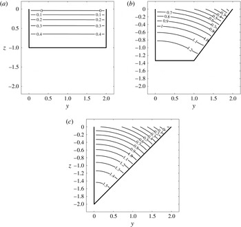
Numerical solutions for
 ${\it\chi}_{2}(y,z)$
in (a) rectangular, (b) trapezoidal and (c) triangular cross-sections with aspect ratio of
 $B_{0}/\overline{h}=2$
, where the mean depth is
 $\overline{h}=A_{0}/B_{0}$
.

4. Applications
To illustrate the capability of the present model, analytical and numerical examples for uniform channels, channels where the geometry changes slowly and channels where changes in cross-section are appreciable within a wavelength are presented in this section. These cases are characterized by
 $\text{d}A_{0}/\text{d}x=0,\;O({\it\epsilon})$
and
 $O(1)$
, respectively. Section 4.1 focuses on the effect of the cross-section geometry on the evolution of a solitary wave in uniform channel. In § 4.2 the numerical results of the present model are compared with laboratory experiments on the evolution of a solitary wave in a rectangular channel with slowly varying width (Chang, Melville & Miles Reference Chang, Melville and Miles1979). In § 4.3, solitary wave propagation in a channel with a rapid contraction is studied.
Following the approach suggested by Liu & Orfila (Reference Liu and Orfila2004), the effects of viscous boundary layer flows on wave decay are introduced in the Boussinesq-type equations. Section 4.4.1 compares the theoretical solutions including the consideration of viscous boundary layer flows to the laboratory experiments for solitary wave shoaling on a sloping beach (Liu et al. Reference Liu, Simarro, Vandever and Orfila2006). Chang et al.’s (Reference Chang, Melville and Miles1979) experimental results are revisited in § 4.4.2 using the model with viscous effects.
4.1. Solitary waves in a uniform channel
Analytical solutions for a solitary wave in a uniform channel with inclined sidewalls can be found in TW97. Here, the solitary wave solutions are briefly discussed for completeness, since they will be used in the following sections as the initial conditions for studying wave propagation in non-uniform channels. For uniform channels of arbitrary cross-sectional geometry, the governing equations for the spanwise-averaged free-surface elevation and the cross-sectional-averaged longitudinal velocity are deduced from (3.19) and (3.43):
 $$\begin{eqnarray}\displaystyle & \displaystyle \frac{\partial \widetilde{{\it\eta}}}{\partial t}+\frac{A_{0}}{B_{0}}\frac{\partial \langle u\rangle }{\partial x}+{\it\epsilon}\frac{A_{0}B_{0}^{\prime }}{B_{0}^{2}}\widetilde{{\it\eta}}\frac{\partial \langle u\rangle }{\partial x}+{\it\epsilon}\frac{\partial }{\partial x}[\langle u\rangle \widetilde{{\it\eta}}]=O({\it\epsilon}^{2},{\it\epsilon}{\it\mu}^{2},{\it\mu}^{4}), & \displaystyle\end{eqnarray}$$
 $$\begin{eqnarray}\displaystyle & \displaystyle \frac{\partial \langle u\rangle }{\partial \hat{t}}+\frac{\partial \widetilde{{\it\eta}}}{\partial \hat{x}}+{\it\epsilon}\langle u\rangle \frac{\partial \langle u\rangle }{\partial \hat{x}}+{\it\mu}^{2}{\it\gamma}\frac{\partial ^{3}\langle u\rangle }{\partial t\partial x^{2}}=O({\it\epsilon}^{2},{\it\epsilon}{\it\mu}^{2},{\it\mu}^{4}). & \displaystyle\end{eqnarray}$$
 $$\begin{eqnarray}\displaystyle & \widetilde{{\it\eta}}=\text{sech}^{2}[K(x-ct)]+O({\it\epsilon},{\it\mu}^{2}), & \displaystyle\end{eqnarray}$$
 $$\begin{eqnarray}\displaystyle & \displaystyle \langle u\rangle =\frac{1}{\sqrt{\overline{h}}}\text{sech}^{2}[K(x-ct)]+O({\it\epsilon},{\it\mu}^{2}), & \displaystyle\end{eqnarray}$$
 $$\begin{eqnarray}K=\frac{1}{2{\it\mu}}\sqrt{\frac{{\it\epsilon}}{\overline{h}{\it\gamma}}\left(\frac{\overline{h}B_{0}^{\prime }}{3B_{0}}-1\right)},\quad c^{2}=\overline{h}-{\it\epsilon}\left(1-\frac{\overline{h}B_{0}^{\prime }}{3B_{0}}\right)\text{Sgn}({\it\gamma}),\quad \overline{h}=\frac{A_{0}}{B_{0}},\end{eqnarray}$$
where
 $\text{Sgn}({\it\gamma})$
denotes the sign of
 ${\it\gamma}$
,
 $K$
is the effective wavenumber,
 $c$
represents the phase speed and
 $\overline{h}$
is the mean depth (see TW97). The solitary wave solution given above is valid only if
 $(\overline{h}B_{0}^{\prime }/3B_{0}-1)/{\it\gamma}>0$
. Since the sign of
 ${\it\gamma}$
depends on cross-sectional geometry and cannot be generalized, the following discussions are restricted to three simple geometries, namely rectangular, triangular and trapezoidal, for which
 ${\it\gamma}<0$
(figure 3). In these cases the parameters of the cross-sectional geometry (embedded in
 ${\it\gamma}$
,
 $B_{0}$
,
 $\overline{h}$
and
 $B_{0}^{\prime }$
) affect the equivalent wavelength and phase speed. However, the phase speed is independent of the magnitude of
 ${\it\gamma}$
. Thus, solitary waves travelling in a channel with outwardly fanning sidewalls at
 $z=0$
, i.e.
 $0<B_{0}^{\prime }<3B_{0}/\overline{h}$
, propagate with longer wavelengths and slower speeds, compared to those in a rectangular channel with
 $B_{0}^{\prime }=0$
. Conversely, in a channel with downwardly fanning sidewalls with
 $B_{0}^{\prime }<0$
, solitary waves have shorter wavelengths and faster wave speeds.
Numerical solutions for
 ${\it\chi}_{2}$
, which are used to compute
 ${\it\gamma}$
and other derived quantities for rectangular, trapezoidal and triangular cross-sections, are shown in figure 3. The cross-sections are characterized by a ratio of
 $B_{0}/\overline{h}=2$
. The trapezoidal and triangular cross-sections are non-symmetric with respect to the
 $x$
-axis. Contour lines of
 ${\it\chi}_{2}$
are perpendicular to the sidewalls whereas on the SWL (
 $z=0$
),
 ${\it\chi}_{2}$
decreases from a maximum value on the vertical walls to a minimum on the sloping walls. The magnitude of the gradient of
 ${\it\chi}_{2}$
increases in
 $z$
, implying higher velocities on the free surface. The coefficients obtained from (3.42) are
 ${\it\gamma}=-0.336$
for the rectangular,
 ${\it\gamma}=-0.496$
for the trapezoidal and
 ${\it\gamma}=-0.632$
for triangular cross-sections.
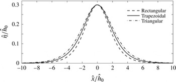
Figure 4 illustrates solitary wave free-surface profiles with
 ${\it\epsilon}=0.3$
in these cross-sections. As predicted, the wavelength is the longest in the triangular channel and shortest for the rectangular cross-section. Since the nonlinearity is the same for all cases, solitary waves travel at different phase speeds solely due to the effect of the sidewall slope,
 $B_{0}^{\prime }$
. The reader is referred to Teng (Reference Teng2000) for a detailed discussion on the effects of cross-sectional geometry on solitary waves of permanent form.
Solitary wave profiles in rectangular, trapezoidal and triangular cross-sections with aspect ratio of
 $B_{0}/\overline{h}=2$
, where the mean depth is
 $\overline{h}=A_{0}/B_{0}$
.

The expression for the velocity components on a cross-sectional plane in a uniform channel can be deduced from (3.35) and (3.36),
 $$\begin{eqnarray}v={\it\mu}^{2}\frac{\partial {\it\chi}_{2}}{\partial y}\frac{\partial \langle u\rangle }{\partial x}\quad \text{and}\quad w={\it\mu}^{2}\frac{\partial {\it\chi}_{2}}{\partial z}\frac{\partial \langle u\rangle }{\partial \hat{x}}.\end{eqnarray}$$
The surface elevation is obtained from (3.37):
 $$\begin{eqnarray}{\it\eta}=\widetilde{{\it\eta}}+{\it\mu}^{2}{\it\eta}_{2},\quad \text{where}\;{\it\eta}_{2}\equiv \left(\widetilde{\left.{\it\chi}_{2}\right|_{z=0}}-\left.{\it\chi}_{2}\right|_{z=0}\right)\frac{\partial ^{2}\langle u\rangle }{\partial t\partial x}.\end{eqnarray}$$
For a rectangular channel, the free-surface elevation
 ${\it\eta}$
is the same as the spanwise-averaged free-surface elevation
 $\widetilde{{\it\eta}}$
since
 ${\it\chi}_{2}$
is independent of
 $y$
(figure 3
a). The spanwise velocity is zero and the vertical velocity varies from a maximum value on the free surface to zero at the bottom. More interesting flow features are found for non-symmetric trapezoidal and triangular cross-sections, where
 ${\it\chi}_{2}$
changes in the spanwise direction (figure 3
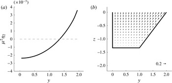
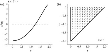
b,c) and so do the surface elevation, velocity and pressure. In fact, at the phase of maximum acceleration, the second-order surface elevation
 ${\it\mu}^{2}{\it\eta}_{2}$
is concave and varies from a minimum value at the vertical sidewall to a maximum value on the inclined sidewalls (figures 5
a and 6
a). At the maximum deceleration phase, the second-order surface elevation becomes convex. The velocity on the cross-section,
 $\boldsymbol{u}_{n}=(v,w)$
, has a maximum value on the inclined sidewalls and diminishes towards the vertical walls on the opposite side of the channel cross-section (figures 5
b and 6
b). It is noted that the velocity on the cross-sectional plane is one order of magnitude smaller than the cross-sectional-averaged longitudinal velocity
 $\langle u\rangle$
in both cases.
(a) The second-order solution for the surface elevation and (b) transverse velocities, for a solitary wave in a trapezoidal channel with aspect ratio of
 $B_{0}/\overline{h}=2$
during maximum acceleration. The magnitude of the velocity is depicted as a small arrow in the bottom right corner. Dashed horizontal line denotes the still level.

(a) The second-order solution for the surface elevation and (b) transverse velocities for a solitary wave in a triangular channel with aspect ratio of
 $B_{0}/\overline{h}=2$
during maximum acceleration. The magnitude of the velocity is depicted as a small arrow in the bottom right corner. Dashed horizontal line denotes the still level.

4.2. Solitary-type wave propagating in a channel of slowly varying width
Chang et al. (Reference Chang, Melville and Miles1979), referred to as C79 hereafter, presented laboratory data and numerical simulations for the evolution of solitary waves in a rectangular channel of constant depth with gradually varying width. Thirty-six experiments were conducted in converging and diverging channels with different initial wave amplitudes. In this section, experimental cases with depths of
 ${\hat{h}}=0.3$
and 0.2 m, for both convergent and divergent channels, are used to check the present theory. Results obtained from TW97’s theory, in which
 ${\it\alpha},{\it\beta}=0$
, are also included for comparison. Recall that TW97’s theory is valid for slow-varying cross-sections, i.e.
 $\text{d}A_{0}/\text{d}x=O({\it\epsilon})$
, whereas in the present theory changes in the area are allowed to be
 $\text{d}A_{0}/\text{d}x=O(1)$
. Note that the effect of energy dissipation due to the wall boundary layer flows has been ignored up to this section; it will be investigated specifically for C79’s experiments in § 4.4.2. For convenience, dimensional quantities are used in this section.
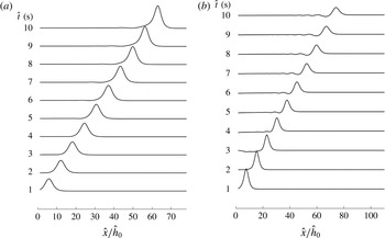
Instantaneous surface elevation for (a) an initial solitary wave of
 ${\it\epsilon}=0.174$
in a converging channel of
 ${\hat{h}}_{0}=0.3~\text{m}$
and (b) an initial solitary wave of
 ${\it\epsilon}=0.259$
in a diverging channel of
 ${\hat{h}}_{0}=0.2~\text{m}$
. Profiles are depicted every 1 s, from
 $\hat{t}=1$
to 10 s.

For the convergent channel the width is defined as
 $$\begin{eqnarray}\hat{B}_{0}(\hat{x})=\left\{\begin{array}{@{}ll@{}}0.45,\quad & -10\leqslant \hat{x}<2.63,\\ 0.45-0.01875(\hat{x}-2.63),\quad & 2.63\leqslant \hat{x}<23.96,\\ 0.05,\quad & 23.96\leqslant \hat{x}<48,\end{array}\right.\end{eqnarray}$$
where
 $\hat{B}_{0}$
and
 $\hat{x}$
are expressed in metres. It is noted that in the laboratory measurements dissipative materials were installed near the end of the converging channel to damp out waves (C79, figure 1). In the present numerical simulations, an additional channel section with uniform width is inserted in the region
 $\hat{x}\geqslant 23.96~\text{m}$
to allow waves propagate out of the computational domain. In the divergent channel, the width is defined as
 $$\begin{eqnarray}\hat{B}_{0}(\hat{x})=\left\{\begin{array}{@{}ll@{}}0.05,\quad & -10\leqslant \hat{x}<2.63,\\ 0.05+0.01875(\hat{x}-2.63),\quad & 2.63\leqslant \hat{x}<26.63,\\ 0.5,\quad & 26.63\leqslant \hat{x}<48.\end{array}\right.\end{eqnarray}$$
The governing equations, (3.19) and (3.43), are solved numerically by using the fourth-order Adams–Bashforth–Moulton method (e.g. Wei and Kirby Reference Wei and Kirby1995). The numerical scheme was tested for a solitary wave propagating in a rectangular channel with uniform cross-section. The present model replicated the results obtained by Wei and Kirby (Reference Wei and Kirby1995) and was found to conserve mass throughout the simulations. Conservation of mass was evaluated with the expression
 $$\begin{eqnarray}R_{(t)}=1-\frac{m_{(t)}}{m_{(0)}},\quad \text{where }m_{(t)}=\int _{-\infty }^{\infty }B_{0}\widetilde{{\it\eta}}\text{d}x\end{eqnarray}$$
is the excess of mass due to the wave at time
 $t$
and
 $m_{(0)}$
is the initial excess of mass. As an example, in the uniform rectangular channel used by Wei and Kirby (Reference Wei and Kirby1995), a value of
 $R_{(160)}=3.2\times 10^{-4}$
was found for a nonlinear parameter of
 ${\it\epsilon}=0.1$
at
 $t=160$
.
In C79, solitary waves were generated by a vertical bulkhead moving with the same velocity as that of fluid particles in the water column under a solitary wave. In the present numerical simulations the solitary wave solutions, given in (4.3) and (4.4), are used as the initial conditions for different cases. For the converging channel, initial solitary waves with nonlinearities of
 ${\it\epsilon}=0.052$
, 0.092, 0.142 and 0.174 are used. The wave crest is always located at
 $\hat{x}=0$
as initial condition. On the other hand, in the diverging channel,
 ${\it\epsilon}=0.088$
, 0.185, and 0.259 centred at
 $\hat{x}=0$
are examined. The no-flux boundary conditions are applied at upstream and downstream boundaries, which are set at
 $\hat{x}=-10~\text{m}$
and
 $\hat{x}=48~\text{m}$
, respectively. The boundaries are sufficiently far from the varying-width section so that their appearance does not affect the solutions inside the varying channel.
4.2.1. Converging channel
Figure 7(a) depicts the evolution of the solitary wave with initial amplitude,
 ${\it\epsilon}=0.174$
. The wave profile gradually evolves from a solitary wave to an asymmetric profile of larger amplitude with a longer tail that increases with travelling distance, which was also observed in the laboratory experiments (C79, figure 7). The long tail actually represents a portion of the reflected waves. Since the channel width changes slowly on the wavelength scale, an incident wave is continuously and slowly reflected from the sidewalls. Therefore, the reflected wave does not have a sharp and identifiable wave crest. However, the total amount of mass contained in the reflected wave could be significant if the incident wave has travelled a long distance (i.e. many wavelengths) as pointed out by Kirby & Vengayil (Reference Kirby and Vengayil1988). The conservation of mass is checked throughout the entire simulation. As an example, for the nonlinear parameter of
 ${\it\epsilon}=0.052$
, a value of
 $R_{(12)}=2.0\times 10^{-7}$
was obtained at
 $\hat{t}=12~\text{s}$
.
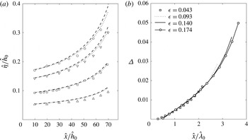
Figure 8(a) shows the local amplitudes of the evolving waves, normalized by the local water depth, along the channel. Experimental results and numerical results obtained with the present and TW97’s theories are included. An increase in wave amplitudes along the channel is clearly observed as the consequence of the reduction in the width, which in the present model is represented by the leading-order term in the conservation of mass equation, i.e.
 $(h/B_{0})(\overline{u}B_{0})_{x}$
, and the second-order terms associated with
 ${\it\alpha}$
and
 ${\it\beta}$
in the momentum equation. The coefficients
 ${\it\alpha}$
and
 ${\it\beta}$
grow significantly as the cross-section becomes narrower since they are proportional to
 $B_{0}^{-2}$
and
 $B_{0}^{-1}$
, respectively, (3.50). Both models consistently overestimate the maximum surface elevation along the channel, though the present model is slightly closer to the experimental data due to the inclusion of the terms associated with
 ${\it\alpha}$
and
 ${\it\beta}$
. It is shown in § 4.4 that the introduction of viscous effects provides a much better agreement between the experiments and the present models.
Numerical results are compared with the experimental data of C79 for the linear converging channel with a mean water depth of
 ${\hat{h}}_{0}=0.3~\text{m}$
. (a) Numerical solutions for the maximum surface elevations for initial solitary waves of
 ${\it\epsilon}=0.043$
, 0.093, 0.140 and 0.174 (from bottom to top), obtained from the present model are depicted by dotted lines. Numerical results obtained from TW97’s model are shown in dashed lines. Experimental data are denoted by triangles for
 ${\it\epsilon}=0.043$
, squares for
 ${\it\epsilon}=0.093$
, inverted triangles for
 ${\it\epsilon}=0.140$
, and circles for
 ${\it\epsilon}=0.174$
. (b) The relative difference between the two models is depicted along the channel; the distance is normalized by the effective wavelength of the incident solitary wave.

The relative difference between the present and TW97 models is presented in figure 8(b). Note that the horizontal axis of this plot is normalized by the effective wavelength of the initial solitary wave. The relative difference is defined as
 $$\begin{eqnarray}{\it\Delta}=\frac{({\it\eta})_{TW}-{\it\eta}}{{\it\eta}},\end{eqnarray}$$
where
 $({\it\eta})_{TW}$
denotes the dimensionless free-surface elevation obtained with TW97’s theory. Note first that the differences are all positive throughout the entire process, implying that the higher-order effects of a narrowing channel cross-section reduce the wave amplitude. The relative differences tend to accumulate as the waves propagate along the channel, following similar curves that are weakly dependent on
 ${\it\epsilon}$
. Since the wavelength of a solitary wave decreases as the wave height increases, for a larger solitary wave the channel appears to be longer, resulting in a larger
 ${\it\Delta}$
value. For example, for the solitary wave of
 ${\it\epsilon}=0.043$
,
 ${\it\Delta}=0.016$
at the end of the channel, where
 $\hat{x}/\hat{{\it\lambda}}_{0}=2.15$
and
 $\hat{{\it\lambda}}_{0}=2{\rm\pi}/\hat{K}$
. On the other hand, for the largest solitary wave of
 ${\it\epsilon}=0.174$
,
 ${\it\Delta}=0.050$
at
 $\hat{x}/\hat{{\it\lambda}}_{0}=3.66$
.
4.2.2. Diverging channel
Typical numerical results for an incident solitary wave of
 ${\it\epsilon}=0.259$
in a diverging channel are shown in figure 7(b). It is clear that the amplitude of the main wave decreases as the channel cross-section widens; thus the dispersive effects become more important and accordingly a dispersive tail arises. These features were also reported by C79, figure 6. Again, the mass conservation has been checked. As an example, for
 ${\it\epsilon}=0.088$
, a value of
 $R_{(12)}=4.0\times 10^{-15}$
was obtained at
 $\hat{t}=12~\text{s}$
.
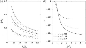
The experimental measurements for the wave amplitudes along the diverging channel are plotted on figure 9(a), together with the numerical results obtained from the present and TW97 theories. Though both theories overestimate the surface elevation along the channel, TW97’s theory appears to match experimental data better. The comparison of theories shows that the contributions from the terms associated with
 ${\it\alpha}$
and
 ${\it\beta}$
cause increases in the amplitudes, and they tend to be stronger with higher nonlinearity. The difference between theories and experimental data is larger than for the converging case. Viscous effects play a significant role in this case, as is later shown in § 4.4.
Numerical results are compared with the experimental data of C79 for the linear diverging channel with a mean water depth of
 ${\hat{h}}_{0}=0.2~\text{m}$
. (a) Maximum surface elevations for initial solitary waves of
 ${\it\epsilon}=0.088$
, 0.185, and 0.259 (from bottom to top) obtained from the present model are denoted by dotted lines. Numerical results obtained from TW97’s model are shown as dashed lines. Experimental data are shown as triangles for
 ${\it\epsilon}=0.088$
, circles for
 ${\it\epsilon}=0.185$
and squares for
 ${\it\epsilon}=0.259$
. (b) The relative difference between the two models along the channel is shown; the distance is normalized by the effective wavelength of the incident solitary wave.

Figure 9(b) shows that the relative difference between the theories increases with longer travelling distance and stronger nonlinearity. Negative values of
 ${\it\Delta}$
imply the present theory provide larger values than TW97 due to the contribution of the new terms. For example, for the smallest solitary wave of
 ${\it\epsilon}=0.088$
,
 ${\it\Delta}=0.022$
at the end of the channel where the wave has travelled roughly 3.94 wavelengths in distance. In the case of the largest wave of
 ${\it\epsilon}=0.259$
, a larger difference between theories is observed, i.e.
 ${\it\Delta}=0.041$
at
 $\hat{x}/\hat{{\it\lambda}}_{0}=6.19$
, since the wave has travelled a longer distance with respect to the incident wave wavelength.
In C79’s experiments, only slowly varying cross-sections are considered. Consequently, the contributions of the new terms containing
 ${\it\alpha}$
and
 ${\it\beta}$
are small, and thus both the present and TW97’s theories provide similar results. The following section shows results for a channel where the cross-section varies significantly within a wavelength.
4.3. Solitary-type wave in a channel with a rapid contraction
Numerical experiments are performed in a channel with a rapid contraction, where the new terms containing
 ${\it\alpha}$
and
 ${\it\beta}$
in the present theory become significant. Since no laboratory experiments for such conditions can be found in the literature, the analysis is focused on the comparison between the present and TW97’s models. In the numerical simulations, rectangular and triangular cross-sections are compared to evaluate the effects of the new coefficients and the sidewall slope on wave properties. To compare results, the mean depth
 $\overline{h}=A_{0}/B_{0}$
and the surface width
 $B_{0}$
are the same for both geometries at any
 $x$
throughout the domain. For a linear contraction, the surface width is defined by
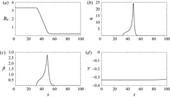
 $$\begin{eqnarray}B_{0}=\left\{\begin{array}{@{}ll@{}}3.\overline{3},\quad & -33.\overline{3}\leqslant x<33.\overline{3},\\ 9.6-0.188x,\quad & 33.\overline{3}\leqslant x<50,\\ 0.2,\quad & 50\leqslant x<100,\end{array}\right.\end{eqnarray}$$
where
 $B_{0}$
and
 $x$
are normalized by the depth (figure 10
a). The maximum and minimum depth-to-width ratios are chosen as
 $B_{0}=3.\overline{3}$
at the entrance and
 $B_{0}=0.2$
at the end of the contraction, satisfying the assumption of comparable depth and widths. With these values, the change of channel width is appreciable within a wavelength, i.e.
 $\text{d}A_{0}/\text{d}x=O(1)$
. The coefficients in the momentum equation for a rectangular channel given by (3.50) are depicted in figure 10(b–d). Coefficients
 ${\it\alpha}$
and
 ${\it\beta}$
are zero in the uniform portion of the channel and increase in the contraction as the section becomes narrower. Compared to the slowly varying case, the magnitudes of these coefficients are one to two orders of magnitude larger, thus their contributions are expected to be more relevant. The coefficient
 ${\it\gamma}$
is a constant throughout the channel.
(a) Channel width and (b–d) coefficients in the momentum equation along a rectangular channel with a rapid contraction.

For the rectangular cross-sections, solitary waves with amplitudes of
 ${\it\epsilon}=0.05$
and 0.1, centred at
 $x=0$
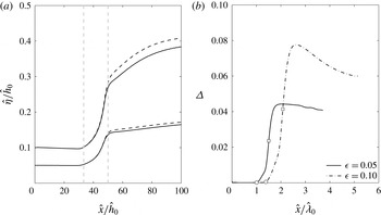
, are used as initial conditions for the numerical experiments. Figure 11(a) shows the comparison of the maximum surface elevation along the channel, obtained by the present and TW97’s models. As expected, the reduction of the cross-section induces a significant increase in the surface elevation during and after the transition, asymptotically approaching a constant value far downstream from the contraction (
 $x>100$
). The contributions of the new terms associated with
 ${\it\alpha}$
and
 ${\it\beta}$
counteract the leading-order amplification caused by the contraction of the channel, therefore amplitudes predicted by the new theory are lower than those of TW97.
Numerical results in a rectangular channel with a rapid contraction. (a) Maximum surface elevations for initial solitary waves of
 ${\it\epsilon}=0.05$
and 0.10. Numerical results from the present model are depicted by solid lines and those from TW97’s theory by dashed lines. Vertical dashed lines denote the beginning and the end of the contraction. (b) The relative difference between the two models is shown. Circles indicate the beginning and squares the end of the contraction.

The relative difference between theories shown in figure 11(b) increases as the wave propagates along the channel. It also increases with larger waves. For instance, for
 ${\it\epsilon}=0.05$
,
 ${\it\Delta}=0.04$
and for
 ${\it\epsilon}=0.01$
,
 ${\it\Delta}=0.07$
at the end of the channel. Note that in these cases the channel transition length is roughly one-half of a wavelength. Although the values of
 ${\it\Delta}$
are comparable to those in the slowly varying channels, the length of the channel contraction section in terms of the wavelength is much shorter.
For the triangular channel, the effect of sidewall slope also plays a role in determining wave evolution. The term associated with
 $B_{0}^{\prime }$
appears in the continuity equation, whereas the coefficients given by (3.55)–(3.57) are reduced to
 $$\begin{eqnarray}{\it\alpha}=\left(\frac{1}{16}-\frac{H^{2}}{3B_{0}^{2}}\right)\left(\frac{\text{d}B_{0}}{\text{d}x}\right)^{2},\quad {\it\beta}=\left(\frac{B_{0}}{16}-\frac{H^{2}}{3B_{0}}\right)\frac{\text{d}B_{0}}{\text{d}x},\quad {\it\gamma}=\frac{B_{0}^{2}}{48}-\frac{H^{2}}{3}.\end{eqnarray}$$
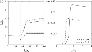
As seen in figure 12(a), the wave shoaling in the triangular channel is milder than that in the rectangular one. The relative difference depicted in figure 12(b) ranges between
 ${\it\Delta}=0.07$
and
 ${\it\Delta}=0.11$
at the end of the channel for
 ${\it\epsilon}=0.05$
and 0.01, respectively. These values are larger than the corresponding cases in the rectangular channel.
Numerical results in a triangular channel with a rapid contraction. (a) Maximum surface elevations for initial solitary waves of
 ${\it\epsilon}=0.05$
and 0.10. Numerical results from the present model are depicted by solid lines and those from TW97’s theory by dashed lines. Vertical dashed lines denote the beginning and the end of the contraction. (b) The relative difference between the two models is shown. Circles indicate the beginning and squares the end of the contraction.

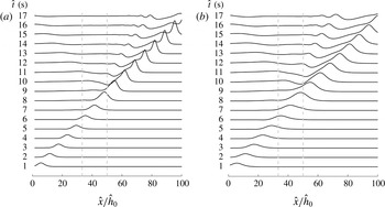
Figure 13 depicts the wave evolution in channels of rectangular and triangular cross-sections during the entire simulation. The initial profiles are slightly different as the effective wavenumber
 $K$
is a function of the cross-sectional geometry. As waves move through the channel contraction, they experience an increase in the surface elevation, evolving from a solitary to an asymmetric profile, followed by a dispersive tail. At the same time small waves are reflected back from the channel contraction, reaching
 $\hat{x}/{\hat{h}}_{0}=0$
at
 $\hat{t}=15{-}17~\text{s}$
. The reflected waves are more detectable since the channel width changes appreciably within the wavelength scale. The main wave grows stronger in the rectangular cross-section channel, whereas the trailing wave train has larger amplitudes in the triangular channel.
Instantaneous surface elevation for an initial solitary wave of
 ${\it\epsilon}=0.05$
in (a) a rectangular and (b) a triangular cross-section of equivalent depth
 ${\hat{h}}_{0}=0.3~\text{m}$
. Profiles are depicted every 1 s, from
 $\hat{t}=1$
to 17 s. Vertical dashed lines denote the beginning and end of the contraction.

4.4. Viscous effects
It is known from the literature that viscous effects could become important in small-scale laboratory experiments (e.g. Liu et al. Reference Liu, Simarro, Vandever and Orfila2006). Indeed, figures 8 and 9 show the large discrepancies between the theoretical predictions and experimental measurements appearing for C79’s experiments. Both C79 and Kirby & Vengayil (Reference Kirby and Vengayil1988) suggested that the discrepancies are caused by viscous dissipation. In this section the effects of laminar boundary layer flows adjacent to the channel boundary are added in the cross-sectional-averaged continuity equation. This approach was developed by Liu & Orfila (Reference Liu and Orfila2004) for the bottom boundary layer and was extended in Liu et al. (Reference Liu, Simarro, Vandever and Orfila2006) to consider the viscous damping of a solitary wave propagating in a rectangular channel, in which both bottom and sidewall boundary layers are considered.
Liu & Orfila (Reference Liu and Orfila2004) showed that the viscous effects generate a flow deficit in the wave propagation direction in bottom boundary layer flows, which in turn induces mass fluxes normal to the boundary into the core region where Boussinesq-type equations are solved. Consequently, in deriving the cross-sectional-averaged equation for conservation of mass, additional mass fluxes along the outer edge of the boundary layer must be added:
 $$\begin{eqnarray}\frac{1}{{\it\varepsilon}}\frac{\partial A}{\partial t}+\frac{\partial }{\partial x}[\langle u\rangle A]=\frac{{\it\delta}}{{\it\mu}}U_{{\it\xi}},\end{eqnarray}$$
where
 $$\begin{eqnarray}{\it\delta}^{2}=\frac{\hat{{\it\nu}}}{\hat{{\it\lambda}}\sqrt{{\hat{g}}{\hat{h}}_{0}}}\end{eqnarray}$$
represents a dimensionless measure of viscous effects, with
 $\hat{{\it\nu}}=10^{-6}~\text{m}^{2}~\text{s}^{-1}$
being the kinematic viscosity of water. Following Liu et al. (Reference Liu, Simarro, Vandever and Orfila2006) for a rectangular channel (figure 2
a), the total flux being transferred from the boundary layer to the core region becomes
 $$\begin{eqnarray}U_{{\it\xi}}(x,t)=\frac{B_{0}+2h}{\sqrt{{\rm\pi}}}\int _{0}^{t}\frac{\partial \langle u(x,{\it\tau})\rangle /\partial x}{\sqrt{t-{\it\tau}}}\text{d}{\it\tau}.\end{eqnarray}$$
Hence, for a rectangular channel with a varying cross-section, the continuity equation (3.19) becomes, to
 $O({\it\epsilon}^{2},{\it\epsilon}{\it\mu}^{2},{\it\mu}^{4})$
,
 $$\begin{eqnarray}\displaystyle & & \displaystyle \frac{\partial \widetilde{{\it\eta}}}{\partial t}+\frac{1}{B_{0}}\frac{\partial }{\partial x}[\langle u\rangle A_{0}]-{\it\epsilon}\frac{B_{0}^{\prime }}{B_{0}^{2}}\widetilde{{\it\eta}}\frac{\partial }{\partial x}[\langle u\rangle A_{0}]+\frac{{\it\epsilon}}{B_{0}}\frac{\partial }{\partial x}[\langle u\rangle B_{0}\widetilde{{\it\eta}}]\nonumber\\ \displaystyle & & \displaystyle \quad -\,\frac{{\it\delta}}{{\it\mu}}\left(\frac{1+2h/B_{0}}{\sqrt{{\rm\pi}}}\right)\int _{0}^{t}\frac{\partial \langle u(x,{\it\tau})\rangle /\partial x}{\sqrt{t-{\it\tau}}}\text{d}{\it\tau}=0.\end{eqnarray}$$
It is necessary to recognize that
 ${\it\delta}=O({\it\epsilon}^{2},{\it\mu}^{4})$
is added to the Boussinesq approximation, so that the viscous effects are slightly weaker than the frequency dispersion and nonlinear effects, but not too small to be neglected. The cross-sectional-averaged momentum equation (3.43) remains unchanged.
The same fourth-order Adams–Bashforth–Moulton method is used to solve the governing equations with the viscous effects, (4.17) and (3.43). The convolution integral representing the viscous term is computed by using the Gauss-Quadrature method. The viscous model is checked with the shoaling of solitary waves over a uniform beach in a rectangular wave channel (Liu et al. Reference Liu, Simarro, Vandever and Orfila2006) in the next section.
4.4.1. Viscous damping of solitary waves in the shoaling zone
The present theory is compared to experimental data obtained by Liu et al. (Reference Liu, Simarro, Vandever and Orfila2006) in a rectangular channel with a sloping beach. Experiments were performed in the 32 m long, 0.6 m wide and 0.9 m deep wave tank in the DeFrees Hydraulics Laboratory at Cornell University. The channel consists of an initial uniform rectangular cross-section of water depth
 ${\hat{h}}=0.15~\text{m}$
and a 1:20 sloping glass beach. Surface elevations were recorded at six locations with a constant spacing of 2.5 m in the constant depth region and of approximately 0.5 m in the shoaling zone. Several solitary waves with different wave amplitudes were generated. At
 $\hat{x}=6.5~\text{m}$
from the wavemaker, solitary waves with
 ${\it\epsilon}=0.091$
, 0.174, 0.270, 0.352 and 0.409 were measured. In the numerical simulations, the water depth is defined by
 $$\begin{eqnarray}{\hat{h}}=\left\{\begin{array}{@{}ll@{}}0.15,\quad & -10\leqslant \hat{x}<19.88,\\ 1.144-0.05\hat{x},\quad & 19.88\leqslant \hat{x}<22,\\ 0.044,\quad & 22\leqslant \hat{x}\leqslant 32,\end{array}\right.\end{eqnarray}$$
where
 ${\hat{h}}$
and
 $\hat{x}$
are expressed in metres. Since the channel cross-section remains a constant, the cross-sectional-averaged equation of mass conservation, (4.17), can be simplified to
 $$\begin{eqnarray}\frac{\partial \widetilde{{\it\eta}}}{\partial t}+\frac{\partial }{\partial x}(\overline{u}[h+{\it\epsilon}\widetilde{{\it\eta}}])-\frac{{\it\delta}}{{\it\mu}}\frac{1+2h/B_{0}}{\sqrt{{\rm\pi}}}\int _{0}^{t}\frac{\langle u\rangle _{x}(x,{\it\tau})}{\sqrt{t-{\it\tau}}}\text{d}{\it\tau}=0.\end{eqnarray}$$
The coefficients in the momentum equation, (3.43), are defined by (3.49). Note that
 ${\it\alpha}=0$
throughout the domain, whereas
 ${\it\beta}=0$
in the constant depth region and decreases over the slope (
 ${\it\beta}\sim h$
). Thus, without considering the viscous effects, TW97’s and the present theory are the same in the uniform section and are different by the term associated with
 ${\it\beta}$
in the shoaling zone. The dispersive coefficient scales as
 ${\it\gamma}\sim h^{2}$
, so the corresponding term becomes smaller in shallower water.
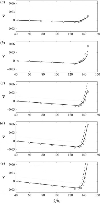
The comparisons between the experimental data and numerical results are presented in figure 14. Both the present model and TW97’s model with viscous effects are computed. Results are shown as the difference between the local wave height and the corresponding value at the first measuring station located at
 $\hat{x}=6.5~\text{m}$
. For convenience, this difference is defined as
 $$\begin{eqnarray}\boldsymbol{{\rm\nabla}}={\it\eta}-({\it\eta})_{6.5}.\end{eqnarray}$$
Maximum surface elevations for solitary waves of
 ${\it\epsilon}=0.091$
(a), 0.174 (b), 0.270 (c), 0.352 (d) and 0.409 (e) at
 $\hat{x}=6.5~\text{m}$
are shown along the wave flume. The results obtained from the present model are depicted by solid lines. Results from TW97’s modified theory are depicted by dashed lines. Both theories include viscous effects. Experimental data by Liu et al. (Reference Liu, Simarro, Vandever and Orfila2006) are shown as circles.

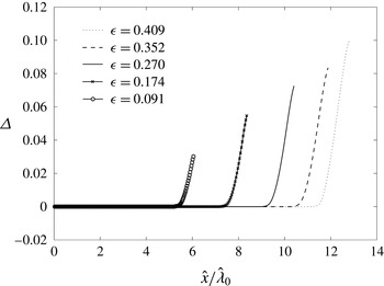
Numerical results from both models are identical and compare reasonably well with the experimental data in the constant depth section, with experimental amplitudes being slightly above the predicted curves. The amplitude decays almost linearly along the uniform section of the flume. In the shoaling zone, the results of the present model are in much better agreement with experimental data because the present model has considered the effects of beach slope accurately. As the nonlinearity increases, the wavelength of the solitary wave becomes shorter. Consequently, the beach slope effects also become more important. The relative difference between the present and TW97’s models (considering viscous effects) also becomes more significant for larger waves, as shown in figure 15. A relative difference between theories of
 ${\it\Delta}=0.03{-}0.1$
appears over the sloping beach for different wave amplitudes.
The relative difference between the solutions obtained from the present and TW97 models in the wave flume is shown for various
 ${\it\epsilon}$
. Note that the distance is normalized by the effective wavelength of the incident solitary wave.

4.4.2. Viscous damping of solitary waves in a converging/diverging channel
In §§ 4.2.1 and 4.2.2, based on the inviscid flow theories, numerical solutions for solitary waves propagating in a converging/diverging channel with a rectangular cross-section are compared with the experimental data in figures 8 and 9, respectively. Results with the consideration of viscous boundary layer effects are shown in this section.
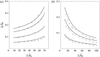
In figure 16 numerical results including viscous boundary layer effects for the linear converging and diverging channels are compared with the experimental data reported in C79. For the converging channel cases (figure 16
a), the new results show excellent agreement for the cases with
 ${\it\epsilon}=0.093,0.140$
and 0.174. The agreement is less impressive for the case of
 ${\it\epsilon}=0.043$
, where the initial wave height is very small. The comparisons for the diverging channel cases are shown on figure 16(b). Although the agreement between the viscous boundary layer theory and the experimental data is improved over that without considering the viscous effects (see figure 9), the improvement is not as significant as in the converging channel case. The causes for this discrepancy are still unknown.
Numerical results that include consideration of viscous boundary layer effects are compared with the experimental data of C79 for linear converging and diverging channels. (a) Maximum surface elevations in the converging channel for initial solitary waves of
 ${\it\epsilon}=0.043$
, 0.093, 0.140 and 0.174 (from bottom to top) obtained from the present model are shown by solid lines. Experimental data are denoted by triangles for
 ${\it\epsilon}=0.043$
, squares for
 ${\it\epsilon}=0.093$
, inverted triangles for
 ${\it\epsilon}=0.140$
and circles for
 ${\it\epsilon}=0.174$
. (b) As in (a) but in the diverging channel for initial solitary waves of
 ${\it\epsilon}=0.088$
, 0.185 and 0.259 (from bottom to top). Experimental data are denoted by inverted triangles for
 ${\it\epsilon}=0.088$
, circles for
 ${\it\epsilon}=0.185$
and squares for
 ${\it\epsilon}=0.259$
.

5. Concluding remarks
A mathematical model for long waves propagating in a straight channel with an arbitrary cross-section is developed. The resulting Boussinesq-type equations are expressed in terms of the cross-sectional-averaged velocity in the longitudinal direction and the spanwise-averaged free-surface elevation. The inclusion of new terms, which depend on the configuration of the channel cross-section, allows rapid changes of the channel geometry in the direction of wave propagation. Thus, the characteristics of wave amplitude amplification/decay and frequency dispersion are affected by the cross-section geometry. Velocity components, pressure and free-surface variation on a cross-section can be calculated once the Boussinesq-type equations are solved. The model is restricted to channels with sidewall slope of order-one, and where depth and width are of the same order.
Two new features of the present model, namely arbitrary channel cross-section and appreciable variation of channel cross-section within the wavelength scale in the direction of wave propagation, have been highlighted by investigating solitary wave propagation in straight channels with rectangular, triangular and trapezoidal cross-sections. Numerical computations in uniform channels show spanwise changes in the surface elevation for trapezoidal and triangular cross-sections, which have been observed earlier in experiments (Sandover & Taylor Reference Sandover and Taylor1962; Peregrine Reference Peregrine1969; Treske Reference Treske1994; Teng & Wu Reference Teng and Wu1997). However, other flow features such as possible wave breaking at the sidewall slopes or cross-wave formation for relatively high Froude numbers (Sandover & Taylor Reference Sandover and Taylor1962; Fenton Reference Fenton1973; Treske Reference Treske1994), cannot be captured by the present theory.
Following Liu & Orfila’s (Reference Liu and Orfila2004) approach, viscous effects from the laminar boundary layer flows are heuristically included in the model. The boundary layer flows are driven by the cross-sectionally averaged pressure gradient in the direction of wave propagation and induce a normal mass flux into the core region, where the velocity field is essentially irrotational. Thus, the cross-sectional-averaged continuity equation is modified by adding the mass flux across the channel boundary. It is shown that the theoretical results that include consideration of viscous boundary layer effects give better agreement with the experimental data by C79 and by Liu et al. (Reference Liu, Simarro, Vandever and Orfila2006). However, in the diverging channel cases, the agreement is less satisfactory. The causes for this discrepancy are still unknown.
The present model could be modified to include some other important features existing in natural systems, such as curvature and channel branching (e.g. Nachbin & Simoes Reference Nachbin and Simoes2012).
Acknowledgements
This work is supported by National Science Foundation grants to Cornell University. P.W. thanks Fulbright, CONICYT and Universidad de Valparaíso for financial assistance in the form of a studentship. The authors also wish to acknowledge referees’ comments that have improved the presentation of the paper.
Appendix A. Derivation of cross-sectional-averaged equations
Although the procedure of deriving the cross-sectional-averaged conservation of mass and momentum equations is straightforward, in the existing literature (Peregrine Reference Peregrine1968; Teng Reference Teng1990) approximations have been adopted that appear to be unnecessary. For completeness, the procedure of derivation and some of the key steps with results are highlighted here.
A.1. Conservation of mass in exact form
The cross-sectional-averaged velocity is defined as
 $$\begin{eqnarray}\langle u\rangle =\frac{1}{A(x,t)}\int _{-s_{r}}^{s_{l}}\int _{-h}^{{\it\epsilon}{\it\eta}}u(x,y,z,t)\text{d}z\text{d}y,\end{eqnarray}$$
in which
 $A(x,t)$
denotes the instantaneous cross-sectional area. Therefore,
 $Q(x,t)=\langle u\rangle A$
represents the volume flux across the cross-section. The conservation of mass requires
 $$\begin{eqnarray}\frac{1}{{\it\epsilon}}\frac{\partial A}{\partial t}+\frac{\partial Q}{\partial x}=\frac{1}{{\it\epsilon}}\frac{\partial A}{\partial t}+\frac{\partial (\langle u\rangle A)}{\partial x}=0,\end{eqnarray}$$
in the dimensionless form.
An alternative derivation is as follows. The exact equation of mass conservation can also be derived by integrating (2.9) in the vertical direction from the bottom
 $z=-h(x,y,t)$
to the surface
 $z={\it\epsilon}{\it\eta}(x,y,t)$
:
 $$\begin{eqnarray}\int _{-h}^{{\it\epsilon}{\it\eta}}\frac{\partial u}{\partial x}\text{d}z+\frac{1}{{\it\mu}^{2}}\left(\int _{-h}^{{\it\epsilon}{\it\eta}}\frac{\partial v}{\partial y}\text{d}z+\int _{-h}^{{\it\epsilon}{\it\eta}}\frac{\partial w}{\partial z}\text{d}z\right)=0.\end{eqnarray}$$
Using the Leibniz rule and the boundary conditions (2.14) and (2.15) yields
 $$\begin{eqnarray}\frac{\partial }{\partial x}\int _{-h}^{{\it\epsilon}{\it\eta}}u\text{d}z+\frac{1}{{\it\mu}^{2}}\frac{\partial }{\partial y}\int _{-h}^{{\it\epsilon}{\it\eta}}v\text{d}z+\frac{\partial {\it\eta}}{\partial t}=0.\end{eqnarray}$$
Defining the depth-averaged velocities as
 $$\begin{eqnarray}\breve{u}=\frac{1}{{\it\epsilon}{\it\eta}+h}\int _{-h}^{{\it\epsilon}{\it\eta}}u\text{d}z,\quad \breve{v}=\frac{1}{{\it\epsilon}{\it\eta}+h}\int _{-h}^{{\it\epsilon}{\it\eta}}v\text{d}z,\end{eqnarray}$$
and the total water depth as
 $H={\it\epsilon}{\it\eta}+h$
, (A 4) becomes
 $$\begin{eqnarray}\frac{1}{{\it\epsilon}}\frac{\partial H}{\partial t}+\frac{\partial }{\partial x}(H\breve{u})+\frac{1}{{\it\mu}^{2}}\frac{\partial }{\partial y}(H\breve{v})=0.\end{eqnarray}$$
Integrating (A 6) from the right-hand boundary
 $y=-s_{r}(x,t)$
to the left-hand boundary
 $y=s_{l}(x,t)$
and using the Leibniz rule yields
 $$\begin{eqnarray}\displaystyle & & \displaystyle \frac{1}{{\it\epsilon}}\frac{\partial }{\partial t}\int _{-s_{r}}^{s_{l}}H\text{d}y+\frac{\partial }{\partial x}\int _{-s_{r}}^{s_{l}}H\breve{u}\text{d}y+H_{(s_{l})}\left[-\frac{1}{{\it\epsilon}}\frac{\partial s_{l}}{\partial t}-\breve{u}_{(s_{l})}\frac{\partial s_{l}}{\partial x}+\frac{1}{{\it\mu}^{2}}\breve{v}_{(s_{l})}\right]\nonumber\\ \displaystyle & & \displaystyle \quad +\,H_{(-s_{r})}\left[-\frac{1}{{\it\epsilon}}\frac{\partial s_{r}}{\partial t}-\breve{u}_{(-s_{r})}\frac{\partial s_{r}}{\partial x}-\frac{1}{{\it\mu}^{2}}\breve{v}_{(-s_{r})}\right]=0,\end{eqnarray}$$
in which the subscripts,
 $(-s_{r})$
and
 $(s_{l})$
, denote the physical quantities being evaluated at
 $y=-s_{r}$
and
 $y=s_{l}$
, respectively. By definition the total water depth at the shoreline vanishes, i.e.
 $H_{(-s_{r})}\;\text{and}\;H_{(s_{l})}=0$
for cross-sections where sidewalls are not vertical. Thus, the last two terms in the equation above vanish. On the other hand, when the channel banks are vertical, the kinematic boundary conditions, (2.16) and (2.17), can be integrated from
 $-h$
to
 ${\it\epsilon}{\it\eta}$
to show that the last two terms in (A 7) also vanish. Thus,
 $$\begin{eqnarray}\frac{1}{{\it\epsilon}}\frac{\partial }{\partial t}\int _{-s_{r}}^{s_{l}}H\text{d}y+\frac{\partial }{\partial x}\int _{-s_{r}}^{s_{l}}H\breve{u}\text{d}y=0.\end{eqnarray}$$
The first integral in the equation is simply the cross-section area whereas the second integral represents the total flux per cross-sectional area. Thus, (A 8) is exactly the same as (A 2). It is noted here that if the effects of viscous boundary layer flows are considered, additional mass fluxes along the outer edge of the boundary layer must be added (see § 4.4).
A.2. Conservation of momentum in exact form
Following a similar averaging procedure, the cross-sectional-averaged momentum equation can be obtained. Namely, the
 $x$
-component of the Euler equations, (2.10), is first integrated in the vertical direction. Upon using the Leibniz rule and the boundary conditions (2.14) and (2.15) the vertical integration yields
 $$\begin{eqnarray}\frac{\partial }{\partial t}\int _{-h}^{{\it\epsilon}{\it\eta}}u\text{d}z+{\it\epsilon}\frac{\partial }{\partial x}\int _{-h}^{{\it\epsilon}{\it\eta}}u^{2}\text{d}z+\frac{{\it\epsilon}}{{\it\mu}^{2}}\frac{\partial }{\partial y}\int _{-b}^{{\it\epsilon}{\it\eta}}uv\text{d}z=-\int _{-h}^{{\it\epsilon}{\it\eta}}\frac{\partial p}{\partial x}\text{d}z.\end{eqnarray}$$
The equation above is then integrated from
 $y=-s_{rl}(x,t)$
to
 $y=-s_{l}(x,t)$
. Using the Leibniz rule and the boundary conditions, (2.16) and (2.17), in the resulting equation yields
 $$\begin{eqnarray}\frac{\partial }{\partial t}\int _{-s_{r}}^{s_{l}}\int _{-h}^{{\it\epsilon}{\it\eta}}u\text{d}z\text{d}y+{\it\epsilon}\frac{\partial }{\partial x}\int _{-s_{r}}^{s_{l}}\int _{-h}^{{\it\delta}{\it\eta}}uu\text{d}z\text{d}y=-\int _{-s_{r}}^{s_{l}}\int _{-h}^{{\it\epsilon}{\it\eta}}\frac{\partial p}{\partial x}\text{d}z\text{d}y,\end{eqnarray}$$
which can be rewritten in terms of the cross-sectional-averaged quantities as
 $$\begin{eqnarray}\frac{\partial }{\partial t}(A\langle u\rangle )+{\it\epsilon}\frac{\partial }{\partial x}(A\langle uu\rangle )=-A\!\left\langle \frac{\partial p}{\partial x}\right\rangle .\end{eqnarray}$$
Equations (A 8) and (A 11) are exact in their present forms. Furthermore, these equations were derived without any additional constraints on the cross-section configuration.
Appendix B. Perturbation expansion
The closure of the system given by (3.4) and (3.5) is accomplished by relating
 $\langle uu\rangle$
and
 $\langle \partial p/\partial x\rangle$
to the spanwise-averaged surface elevation
 $\tilde{{\it\eta}}$
, and the cross-sectional-averaged velocity,
 $\langle u\rangle$
. To accomplish this objective, the dimensionless physical variables are expanded as power series of
 ${\it\mu}^{2}$
, assuming the velocity components on the cross-section are comparable to, but smaller than the longitudinal velocity. These expansions are given in (3.8)–(3.12) and will not be repeated here. From (3.10) the following results can be readily deduced:
 $$\begin{eqnarray}\langle u\rangle =u_{1}+{\it\mu}^{2}\langle u_{2}\rangle +O({\it\mu}^{4}),\quad \langle u\rangle \langle u\rangle =u_{1}^{2}+2{\it\mu}^{2}u_{1}\langle u_{2}\rangle +O({\it\mu}^{4})\end{eqnarray}$$
and
 $$\begin{eqnarray}uu=u_{1}^{2}+2{\it\mu}^{2}u_{1}u_{2}+O({\it\mu}^{4}),\quad \langle uu\rangle =u_{1}^{2}+2{\it\mu}^{2}u_{1}\langle u_{2}\rangle +O({\it\mu}^{4}).\end{eqnarray}$$
Thus,
 $$\begin{eqnarray}\langle uu\rangle =\langle u\rangle \langle u\rangle +O({\it\mu}^{4}).\end{eqnarray}$$
To find an expression for
 $\langle \partial p/\partial x\rangle$
, the perturbation expansions are substituted into the Bernoulli equation (2.13) to obtain
 $$\begin{eqnarray}\frac{\partial {\it\phi}_{1}}{\partial t}+{\it\mu}^{2}\frac{\partial {\it\phi}_{2}}{\partial t}+\frac{1}{2}{\it\epsilon}u_{1}^{2}+p+\frac{z}{{\it\epsilon}}=O({\it\epsilon}^{2},{\it\epsilon}{\it\mu}^{2},{\it\mu}^{4}).\end{eqnarray}$$
Taking the derivative of the equation above with respect to
 $x$
first and averaging the resulting equation over the cross-section of the channel yields
 $$\begin{eqnarray}\frac{\partial ^{2}{\it\phi}_{1}}{\partial x\partial t}+{\it\mu}^{2}\left\langle \frac{\partial ^{2}{\it\phi}_{2}}{\partial x\partial t}\right\rangle +\frac{1}{2}{\it\epsilon}\frac{\partial }{\partial x}(u_{1}^{2})+\left\langle \frac{\partial p}{\partial x}\right\rangle =O({\it\epsilon}^{2},{\it\epsilon}{\it\mu}^{2},{\it\mu}^{4}).\end{eqnarray}$$
Evaluating the Bernoulli equation (B 4) at the surface
 $z={\it\epsilon}{\it\eta}$
yields
 $$\begin{eqnarray}\frac{\partial {\it\phi}_{1}}{\partial t}+{\it\mu}^{2}\left.\frac{\partial {\it\phi}_{2}}{\partial t}\right|_{z={\it\epsilon}{\it\eta}}+\frac{1}{2}{\it\epsilon}u_{1}^{2}+{\it\eta}=O({\it\epsilon}^{2},{\it\epsilon}{\it\mu}^{2},{\it\mu}^{4}).\end{eqnarray}$$
Note that
 ${\it\phi}_{1}$
and
 $u_{1}$
are constants at the cross-section and the atmospheric pressure on the free surface has been assumed to be zero. The second term in the equation above is evaluated on the free surface
 $z={\it\epsilon}{\it\eta}$
and can be approximated by the corresponding term evaluated on the SWL
 $z=0$
, i.e.
 $$\begin{eqnarray}\left.\frac{\partial {\it\phi}_{2}}{\partial t}\right|_{z={\it\epsilon}{\it\eta}}=\left.\frac{\partial {\it\phi}_{2}}{\partial t}\right|_{z=0}+O({\it\epsilon}).\end{eqnarray}$$
Therefore, (B 6) becomes
 $$\begin{eqnarray}\frac{\partial {\it\phi}_{1}}{\partial t}+{\it\mu}^{2}\left.\frac{\partial {\it\phi}_{2}}{\partial t}\right|_{z=0}+\frac{1}{2}{\it\epsilon}u_{1}^{2}+{\it\eta}=O({\it\epsilon}^{2},{\it\epsilon}{\it\mu}^{2},{\it\mu}^{4}).\end{eqnarray}$$
Taking the spanwise average across the still water surface, (3.7), of the above equation, and then taking the derivative of the resulting equation with respect to
 $x$
yields
 $$\begin{eqnarray}\frac{\partial ^{2}{\it\phi}_{1}}{\partial x\partial t}+{\it\mu}^{2}\frac{\partial }{\partial x}\left(\widetilde{\left.\frac{\partial {\it\phi}_{2}}{\partial t}\right|_{z=0}}\right)+\frac{1}{2}{\it\epsilon}\frac{\partial }{\partial x}(u_{1}^{2})+\frac{\partial \widetilde{{\it\eta}}}{\partial x}=O({\it\epsilon}^{2},{\it\epsilon}{\it\mu}^{2},{\it\mu}^{4}).\end{eqnarray}$$
Subtracting (B 9) from (B 5) yields
 $$\begin{eqnarray}\left\langle \frac{\partial p}{\partial x}\right\rangle =\frac{\partial \widetilde{{\it\eta}}}{\partial x}+{\it\mu}^{2}\left[\frac{\partial }{\partial x}\left(\widetilde{\left.\frac{\partial {\it\phi}_{2}}{\partial t}\right|_{z=0}}\right)-\left\langle \frac{\partial ^{2}{\it\phi}_{2}}{\partial x\partial t}\right\rangle \right]+O({\it\epsilon}^{2},{\it\epsilon}{\it\mu}^{2},{\it\mu}^{4}).\end{eqnarray}$$
The last term in the equation above can be approximated using
 $\langle \,f\rangle =\overline{f}+O({\it\epsilon})$
. Thus, the cross-sectional-averaged momentum equation can be deduced by substituting (B 10) and (A 8) into (A 11),
 $$\begin{eqnarray}\frac{\partial \langle u\rangle }{\partial t}+{\it\epsilon}\frac{\partial \langle u\rangle \langle u\rangle }{\partial x}+\frac{\partial \widetilde{{\it\eta}}}{\partial x}+{\it\mu}^{2}\left[\frac{\partial }{\partial x}\left(\widetilde{\left.\frac{\partial {\it\phi}_{2}}{\partial t}\right|_{z=0}}\right)-\overline{\frac{\partial ^{2}{\it\phi}_{2}}{\partial x\partial t}}\right]=O({\it\epsilon}^{2},{\it\epsilon}{\it\mu}^{2},{\it\mu}^{4}),\end{eqnarray}$$
Appendix C. Expressions for the cross-section area
The instantaneous cross-sectional area
 $A(x,t)$
is expressed as the sum of the cross-sectional area at the quiescent state
 $A_{0}(x)$
and the contribution due to wave motions (see (3.1) and (3.2)):
 $$\begin{eqnarray}A=A_{0}+{\it\epsilon}\int _{-b_{r}}^{b_{l}}{\it\eta}\text{d}y+\int _{-s_{r}}^{-b_{r}}({\it\epsilon}{\it\eta}-h)\text{d}y+\int _{b_{l}}^{s_{l}}({\it\epsilon}{\it\eta}-h)\text{d}y,\end{eqnarray}$$
where the limits of integration are defined in figure 1, and the first integral on the right-hand side is, by definition,
 $$\begin{eqnarray}\int _{-b_{r}}^{b_{l}}{\it\eta}\text{d}y=B_{0}\widetilde{{\it\eta}}.\end{eqnarray}$$
In the regions
 $-s_{r}<y<-b_{r}$
and
 $b_{l}<y<s_{l}$
, the free surface is approximated by
 ${\it\eta}=\widetilde{{\it\eta}}$
and the bank slope is assumed to be linear above the SWL (figure 17). Thus, the second and third integrals in (C 1) are approximated as
 $$\begin{eqnarray}\left[\int _{-s_{r}}^{-b_{r}}({\it\epsilon}{\it\eta}-h)\text{d}y+\int _{b_{l}}^{s_{l}}({\it\epsilon}{\it\eta}-h)\text{d}y\right]\sim \frac{{\it\epsilon}^{2}}{2}\left.\left\{-\frac{\text{d}y^{r}}{\text{d}z}\right|_{z=0}+\left.\frac{\text{d}y^{l}}{\text{d}z}\right|_{z=0}\right\}\widetilde{{\it\eta}}^{2},\end{eqnarray}$$
where the terms in curly brackets represent the sidewall slopes at the SWL at both sides of the channel and are assumed to be
 $O(1)$
or smaller. For convenience these terms are lumped together and referred to as
 $B_{0}^{\prime }$
. The cross-sectional area is, therefore, approximated as
 $$\begin{eqnarray}A=A_{0}+{\it\epsilon}B_{0}\widetilde{{\it\eta}}+{\it\epsilon}^{2}\frac{B_{0}^{\prime }}{2}\widetilde{{\it\eta}}^{2}+O({\it\epsilon}^{2}{\it\mu}^{2},{\it\epsilon}^{3}).\end{eqnarray}$$
Definition of components of the cross-section area.