

I. INTRODUCTION
One of the authors has recently demonstrated that a maximum-likelihood structure analysis and appropriate error estimation can be achieved simply by the Rietveld method (Rietveld, Reference Rietveld1969), when the powder diffraction intensity data are collected with a measurement system composed of a two-dimensional (2D) X-ray detector and convergent X-ray beam supplied by a synchrotron light source (Ida, Reference Ida2016). Since the Rietveld method is a least-squares fitting of a parametric model to powder diffraction data, the errors of the optimized parameters can be evaluated, if the statistical errors are known in the observed powder diffraction intensity data.
In that study, the authors have analyzed the diffraction intensity data from a standard powder of lanthanum hexaboride, LaB6 (NIST SRM660b) filled in a 0.1 mm capillary tube, the observed peak profile of which is considered to be close to the overall instrumental function of the measurement system. Slight asymmetry of the peak profile was detected, and the profile was well reproduced by the density function of gamma or beta probability distribution.
In the practical implementation of the Rietveld method, truncation of the model peak profile function is usually applied for the purpose of saving the computing time, but it causes discontinuity of the calculated diffraction intensities, when the profile function has non-zero values for infinite data range. If the beta-distribution peak profile model can be applied, the discontinuity caused by truncation can be avoided, because the function has non-zero values only in a finite range of the variable.
II. THEORETICAL
A. Gamma-distribution peak profile model
Firstly, the authors define a peak profile model given by the probability density function of the gamma distribution as a special case of a beta distribution model. The normalized formula of the gamma-distribution peak profile model with the variable x, average position x Γ, standard deviation σ Γ, and skewness χ Γ is given by
 $$\eqalign{& f_{\rm \Gamma} (x;x_{\rm \Gamma}, \sigma _{\rm \Gamma}, \chi _{\rm \Gamma} ) = \cr & \quad \left\{ {\matrix{ {\,f_{{\rm \Gamma D}}( - x + x_{\rm \Gamma} + {\rm \Delta} x_{\rm \Gamma}, b_{\rm \Gamma}, \alpha _{\rm \Gamma} )} & {[\chi _{\rm \Gamma} \lt 0]} \cr {\displaystyle{1 \over {\sqrt {2\pi} \sigma _{\rm \Gamma}}} {\rm exp}\left[ { - \displaystyle{{{(x - x_{\rm \Gamma} \; )}^2} \over {2\sigma _{\rm \Gamma} ^2}}} \right]} & {[\chi _{\rm \Gamma} = 0]} \cr {\,f_{{\rm \Gamma D}}(x - x_{\rm \Gamma} - {\rm \Delta} x_{\rm \Gamma}, b_{\rm \Gamma}, \alpha _{\rm \Gamma} )} & {[\chi _{\rm \Gamma} \gt 0],} \cr}} \right.} $$
where f ΓD(x, b, α) is the well-known probability density function of the gamma distribution given by
 $$f_{{\rm \Gamma D}}(x,b,\alpha ) = \left\{ {\matrix{ {\displaystyle{{x^{\alpha - 1}{\rm e}^{ - x/b}} \over {{\rm \Gamma} (\alpha )b^\alpha}}} & {[x \gt 0]} \cr 0 & {[x \le 0],} \cr}} \right.$$
where Γ(α) is the gamma function defined by
 $${\rm \Gamma} (\alpha ) \equiv \int_0^\infty {t^{\alpha - 1}} {\rm e}^{ - t}{\rm d}t,$$
and the parameters Δx Γ, b Γ, and α Γ in Eq. (1) are defined from σ Γ and χ Γ by
 $${\rm \Delta} x_{\rm \Gamma} \equiv \alpha _{\rm \Gamma} b_{\rm \Gamma}, $$
 $$b_{\rm \Gamma} \equiv \displaystyle{{\left \vert {\chi _{\rm \Gamma}} \right \vert \sigma _{\rm \Gamma}} \over 2},$$
 $$\alpha _{\rm \Gamma} \equiv \displaystyle{4 \over {\chi _{\rm \Gamma} ^2}}. $$
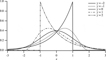
The gamma-distribution peak profile model has non-zero value only in the semi-infinite range of (−∞, x Γ + Δx Γ) for χ Γ < 0 or (x Γ − Δx Γ, + ∞) for χ Γ > 0, and the profile approaches to the Gaussian function for χ Γ → ±0 and α Γ → ∞. The kurtosis (excess) of the gamma-distribution profile model is given by
 $$\varepsilon _{\rm \Gamma} = \displaystyle{6 \over {\alpha _{\rm \Gamma}}} = \displaystyle{{3\chi _{\rm \Gamma} ^2} \over 2}.$$
The profile of the gamma-distribution peak profile function calculated for x Γ = 0, σ Γ = 1, and χ Γ = −2, −1, 0, 1, 2 are shown in Figure 1. The gamma-distribution profile for χ Γ = ±2 is identical to the truncated exponential function, and singularity appears at the edge point for |χ Γ| ≥ 2. Since the gamma-distribution function in the form of Eq. (2) is numerically unstable for χ Γ ≅ 0, a modified formula given by
 $$\eqalign{& f_{{\rm \Gamma D}}(x,b,\alpha ) \equiv \cr & \quad \left\{ {\matrix{ {\displaystyle{1 \over b}{\rm exp}\left[ {(\alpha - 1)\;{\rm ln}\displaystyle{x \over b} - \displaystyle{x \over b} + {\rm ln\Gamma (}\alpha {\rm )}} \right]} & {[x \gt 0],} \cr 0 & {[x \le 0]} \cr}} \right.} $$
would be favorable, when a library function that returns the logarithm of the gamma function, ln Γ(x), is available.
Gamma-distribution peak profile calculated for the average location of zero, standard deviation of unity, and skewness of −2, −1, 0, 1, 2.

B. Beta-distribution peak profile model
The normalized formula of the beta-distribution peak profile model with the variable x, average position
 $x_{\rm B}$
, standard deviation
 $\sigma _{\rm B}$
, an asymmetry parameter γ, and a collapse parameter δ, is given by
 $$\eqalign{& f_{\rm B}(x;x_{\rm B},\sigma _{\rm B},\gamma ,\delta ) = \cr & \quad \left\{ {\matrix{ {\displaystyle{{\rm1 } \over {b_{\rm \Gamma }}}\; f_{{\rm BD}}\left( {\displaystyle{{x - x_{\rm B} + {\rm \Delta }x_{\rm B}} \over {b_{\rm \Gamma }}},\alpha _{{\rm B},}\;\beta _{\rm B}} \right)} & {[0 < \delta ]} \cr {\,f_{\rm \Gamma }(x;x_{\rm B},\sigma _{\rm B},\gamma )} & {[\delta = 0]} \cr } } \right.} $$
where
 $f_{{\rm BD}}(x,\alpha, \beta )$
is the density function of the beta distribution formally defined by
 $$f_{{\rm BD}}(x,\alpha, \beta ) \equiv \left\{ {\matrix{ {\displaystyle{{x^{\alpha - 1}{(1 - x)}^{\beta - 1}} \over {{\rm B}(\alpha, \beta )}}} & {[0 \lt x \lt 1],} \cr 0 & {[x \le 0,\; 1 \le x]} \cr}} \right.$$
where
 ${\rm B}(\alpha, \beta )$
is the beta function defined by
 $${\rm B}(\alpha, \beta ) \equiv \int_0^1 {t^{\alpha - 1}} (1 - t)^{\beta - 1}{\rm d}t = \displaystyle{{{\rm \Gamma (}\alpha {\rm )\Gamma} (\beta )} \over {{\rm \Gamma (}\alpha {\rm +}{\rm \beta )}}}.$$
As the numerical calculation of the probability density function
 $f_{{\rm BD}}(x,\alpha, \beta )$
expressed by Eqs (10) and (11) becomes unstable for large values of α and β, the use of an alternative formula,
 $$f_{{\rm BD}}(x,\alpha, \beta ) \equiv \left\{ {\matrix{ {\exp [\ln \;f_{{\rm BD}}(x,\alpha, \beta )]} & {[0 \lt x \lt 1],} \cr 0 & {[x \le 0,\; 1 \le x]} \cr}} \right.$$
 $$\ln \;f_{{\rm BD}}(x,\alpha, \beta ) = (\alpha - 1)\ln x + (\beta - 1)\ln (1 - x)$$
 $$+ \ln {\rm \Gamma} (\alpha {\rm \;+\;}\beta ) - \ln \;{\rm \Gamma} (\alpha ) - \ln \;{\rm \Gamma} (\beta ),$$
would be preferable for practical implementation.
The parameters
 ${\rm \Delta} x_{\rm B}$
,
 $b_{\rm B},\alpha _{\rm B}$
, and
 ${\rm \;} \beta _{\rm B}$
in Eq. (9) are defined from
 $\sigma _{\rm B}$
, γ, and δ by
 $${\rm \Delta} x_{\rm B} \equiv \displaystyle{{\alpha _{\rm B}b_{\rm B}} \over {\alpha _{\rm B} + {\rm \;} \beta _{\rm B}}},$$
 $$b_{\rm B} \equiv (\alpha _{\rm B} + {\rm \;} \beta _{\rm B})\sqrt {\displaystyle{{\alpha _{\rm B} + {\rm \;} \beta _{\rm B} + 1} \over {\alpha _{\rm B}\beta _{\rm B}}}} \sigma _{\rm B},$$
 $$\alpha _{\rm B} \equiv \left[ {\displaystyle{4 \over {(\gamma + \left \vert \gamma \right \vert + \delta ^2)}}} \right]^2,$$
 $$\beta _{\rm B} \equiv \left[ {\displaystyle{4 \over {(\gamma - \left \vert \gamma \right \vert - \delta ^2)}}} \right]^2\;. $$
The skewness of the beta-distribution peak profile model is given by
 $$\chi _{\rm B} = \displaystyle{{2(\beta _{\rm B} - \alpha _{\rm B})} \over {\alpha _{\rm B} + \beta _{\rm B} + 2}}\sqrt {\displaystyle{{\alpha _{\rm B} + \beta _{\rm B} + 1} \over {\alpha _{\rm B}\beta _{\rm B}}}}, $$
and the kurtosis of the peak model is given by
 $$\varepsilon _{\rm B} = \displaystyle{{6\left[ {{(\beta _{\rm B} - \alpha _{\rm B})}^2(\alpha _{\rm B} + \beta _{\rm B} + 1) - \alpha _{\rm B}\beta _{\rm B}(\alpha _{\rm B} + \beta _{\rm B} + 2)} \right]} \over {\alpha _{\rm B}\beta _{\rm B}(\alpha _{\rm B} + \beta _{\rm B} + 2)(\alpha _{\rm B} + \beta _{\rm B} + 3)}}.$$
Note that the beta-distribution peak profile model for 0 < δ has non-zero values only in the finite range of
 $(x_{\rm B} - {\rm \Delta} x_{\rm B},x_{\rm B} + {\rm \Delta} {x}^{\prime}_{\rm B})$
, where the parameter to determine the upper bound
 ${\rm \Delta} {x}^{\prime}_{\rm B}$
is given by
 $${\rm \Delta} {x}^{\prime}_{\rm B} \equiv \displaystyle{{\beta _{\rm B}b_{\rm B}} \over {\alpha _{\rm B} + {\rm \;} \beta _{\rm B}}}.$$
The beta-distribution peak profile model approaches to the gamma-distribution peak profile model for δ → 0.
The parameter γ that determines the asymmetry of the beta-distribution model is generally different from the skewness of the function
 $\chi _{\rm B}$
, but it coincides with the skewness at the gamma-distribution limit, that is,
 $$\mathop {\lim} \limits_{\delta \to 0} \chi _{\rm B} = \gamma, $$
and it is assured that the beta-distribution peak profile becomes symmetric for γ = 0.
The profile of the beta-distribution peak profile calculated for x Γ = 0, σ Γ = 1, γ = 0, and δ = 0, 1.0, 1.5, 2.0, 2.5 are shown in Figure 2. The kurtosis of the beta-distribution profile can be changed by varying the collapse parameter δ. The sharpest profile among the symmetric beta-distribution profile system is Gaussian at δ = 0, and the profile becomes more collapsed by increasing the value of δ. The symmetric beta-distribution profile becomes rectangular at δ = 2, and then over-collapsed bimodal profile for δ > 2.
Beta-distribution peak profile calculated for the average location of zero, standard deviation of unity, no asymmetry, and collapse parameter of 0, 1.0, 1.5, 2.0, and 2.5.

III. EXPERIMENAL
A. Apparatus
A powder diffraction measurement system constructed on a beam-line BL5S2 at Aichi Synchrotron Radiation Center in Seto, Japan, has been modified for extensive use of 2D X-ray detectors. Four flat 2D detectors (Dectris, PILATUS-100K) are mounted on the movable stages on supporting rods radially attached to the 2Θ-wheel of the goniometer (Huber, 401–440) with the interval of 25°. Any camera length from 340 to 1000 mm can be applied, when the detectors are located on the meridian positions (see Figure 3).
(Colour online) Schematic illustration of the powder diffraction measurement system on the beam line BL5S2 at AichiSR, when the detectors are located at the meridian positions.

The measurement system has also been designed to enable one-shot collection of whole powder diffraction data with the four PILATUS-100K detectors by a simple operation, just rotating the eccentric rod to support the detectors by 180° (see Figure 4). The rotation mechanism is also intended to incline the detector slightly, in order to avoid a leaping behavior of data sampling with squarely arranged detector pixels at the diffraction angles near 90°. It has also been found that the intentional inclination of the square 2D detector also effectively reduces the effect of extraordinary output from the edge pixels of the readout chips of the PILATUS detector, which may occur when the correction (Kraft et al., Reference Kraft, Bergamaschi, Brönnimann, Dinapoli, Eikenberry, Graafsma, Henrich, Johnson, Kobas, Mozzanica, Schlepüz and Schmitt2009) does not work well.
(Colour online) Schematic illustration of the powder diffraction measurement system on the beam line BL5S2 at AichiSR, when the detectors are located at the camera length of 170 mm, which enables to obtain whole powder diffraction data ranging 0 ≤ 2θ ≤ 110° at once.

2D powder diffraction intensity data are reduced to 1D format of powder diffraction data by a pixel mapping method originally proposed for analyzing powder XRD spectra by Sulyanov et al. (Reference Sulyanov, Popov and Kheiker1994), which also enables evaluation of standard uncertainties about the reduced intensity data (Ida, Reference Ida2016).
B. Measurement
The monochromator of the beamline was adjusted to provide the X-ray beam of 12.4 keV in photon energy, 1.0 Å in wavelength. The storage ring was operated at the acceleration voltage of 1.2 GeV and the ring current was kept 300 mA.
Standard powder of lanthanum hexaboride (NIST SRM660b) was used as received. The powder was filled into a glass capillary tube (Hilgenberg, Mark-tube, #14) of 0.1 mm in diameter. The capillary specimen was rotated at the speed of 1 revolution min−1 during the diffraction measurement.
Four flat 2D detectors were simultaneously used for data collection. The camera length R defined as the distance of the foot of a perpendicular on the detector face from the specimen was estimated at 340.77, 340.28, 339.75, and 340.55 mm for each of the four detectors.
The diffraction data were collected at the goniometer angles of 2Θ = 0°, 12.5°, and 25° with the exposure time of 1 min for each. The 2D diffraction data were mapped onto the diffraction angles of 0.01° step, and combined by the method previously reported (Ida, Reference Ida2016), where the differences in intensities from the different detectors were linearly adjusted.
IV. RESULTS
Figure 5(a) shows the combined diffraction intensities from LaB6 powder recorded with four PILATUS detectors positioned at the goniometer angles of 2Θ = 0°, 12.5°, and 25° for No.1, 2Θ = 25°, 37.5°, and 50° for No. 2, 2Θ = 50°, 62.5°, 75° for No. 3, and 2Θ = 75°, 87.5°, and 100° for No. 4 detectors. In total 38 reflection peaks of LaB6 have been detected.
(Colour online) (a) Observed average pixel intensities of LaB6 and (b) calculated curve composed of 38 beta-distribution profile (δ = 0.5) with a background function. (c) The standard deviation estimated for the pixel intensities and (d) the difference plot.

Each of the reflection peaks has been extracted and analyzed by applying the beta-distribution profile model. When the collapse parameter δ is treated as an adjustable parameter, it tends to approach to zero for most of the peaks. The authors then fixed the collapse parameter to be δ = 0.5 in this analysis, but no significant difference has been detected. Typical results of the profile fitting are shown in Figure 6. Double-peak profile of the standard deviation, naturally assigned to the propagation of the horizontal error (Ida, Reference Ida2016), is commonly seen in all the observed peaks.
(Colour online) Results of profile fitting of a beta-distribution profile model to (a) 100, (b) 420, and (c) 622-reflection peaks of LaB6.

The certified lattice parameter of NIST SRM660b for a temperature 22.5 °C, a = 4.15 689 (8) Å is assumed, and the wavelength of the X-ray is calculated from each of the peak locations. The values of wavelength formally calculated are plotted in Figure 7(a). No systematic behavior has been detected, but the length of the error-bars appears to be under-estimated. It is likely that additional errors have been introduced on the mapping and connection of data from different detectors. Assuming the unknown statistical errors are dominant, the wavelength of the source X-ray will formally be estimated at λ = 0.999 429 (2) Å, if the standard error attached to the certified value of NIST SRM660b is neglected. It should be noted that the precision of the estimated wavelength is formally ten times more than that of the certified lattice parameter of the standard sample.
(Colour online) (a) Wavelength calculated from the peak location, (b) peak width as the standard deviation σ, and (c) skewness χ of the profile, optimized by profile fitting with the beta-distribution model.

Figure 7(b) shows the peak width estimated as the standard deviation σ for each peak. The peak width slightly increases at the higher diffraction angles. When this trend is connected with the effect of crystallite size broadening or spectroscopic distribution of the source X-ray, the peak width should be modeled by
 $$\sigma = \sqrt {\sigma _0^2 + \sigma _1^2 \;{\tan} ^2\;\theta}, $$
where σ 0 and σ 1 are adjustable parameters (Caglioti et al., Reference Caglioti, Paoletti and Ricci1958). As the errors about the peak width σ estimated by the profile fitting also appear to be too small as compared with the observed deviation, the initial error values are adjusted to match the standard deviation of the residuals by multiplying a constant factor. After the adjustment of the error values, the parameters are estimated at σ 0 = 0.01 335 (7)° and σ 1 = 0.0082(3)°. The estimated value of the constant term of the standard deviation 0.01 335 (7)° is comparable with the nominal resolution of 0.029°, determined by the pixel size of 0.172 mm and the camera length of 340 mm. When the value of the first-order term σ 1 = 0.0082(3)° is thoroughly assigned to the spectroscopic broadening, the relative spectral width of the source X-ray is estimated to be Δλ/λ = 7.2(3) × 10−5, which is still narrower than the corresponding value Δλ/λ = 1.208(11) × 10−4 of Cu Kα 1 emission (Deutsch et al., Reference Deutsch, Förster, Hölzer, Härtwig, Hämäläinen, Kao, Huotar and Diamant2004).
The values of skewness χ of the peak profile calculated by Eqs (16)–(18) are plotted in Figure 7(c). It is not very clear, but the absolute value of the skewness looks slightly increased at higher angles, which may be caused by asymmetry of the spectroscopic profile of the source X-ray. When the skewness is fitted by
 $$\chi = \chi _1\tan \theta, $$
where χ 1 is the adjustable parameter, it has been optimized to be χ 1 = −0.269(19).
After all the peak intensities are excluded from the source data, 60th-order Fourier cosine expansion was applied to the background intensities. Figure 5(b) shows the intensity data, calculated just by adding the background function and 38 beta-distribution peak profile, individually optimized to each diffraction peak. The fitting residuals shown in Figure 5(d) look larger than the errors estimated by the pixel mapping method, shown in Figure 5(c), which also suggests that there are still unknown errors or statistical variation of the source or processed data.
The R-factors for overall intensity simulation are estimated at R wP = 4.6% and R P = 3.7%.
V. CONCLUSION
Mathematical formulas of gamma and beta-distribution peak profile models are proposed. The peak position, width and asymmetry of both the models are unambiguously defined by the average, standard deviation and skewness. As the beta-distribution model has non-zero values in finite range of the variable, the discontinuity caused by truncation of a profile function can be avoided, given that the observed peak profile is modeled by the beta-distribution function.
The diffraction data of thin capillary sample of LaB6 powder have been collected with four flat 2D detectors on the beamline BL5S2 at Aichi Synchroton Radiation Center (Seto, Aichi Prefecture, Japan) and combined to a series of powder diffraction intensity data. Total diffraction data have been simulated by a fitting method applying the beta-distribution profile model. Overall R-factors have been estimated at R wP = 4.6% and R P = 3.7%.