1. Introduction
Gravity-driven granular flows over an inclined plane have significant implications for geophysical and industrial applications, such as rock avalanches, debris flows and the transport of bulk materials (Goldhirsch Reference Goldhirsch2003; Forterre & Pouliquen Reference Forterre and Pouliquen2008; Kamrin et al. Reference Kamrin, Hill, Goldman and Andrade2024). Although recent decades have seen many advances in the rheology (Jop, Forterre & Pouliquen Reference Jop, Forterre and Pouliquen2006; Gaume, Chambon & Naaim Reference Gaume, Chambon and Naaim2020; Kim & Kamrin Reference Kim and Kamrin2020) and flow rule of granular materials (Pouliquen Reference Pouliquen1999; Börzsönyi & Ecke Reference Börzsönyi and Ecke2007; Wu et al. Reference Wu, Pähtz, Guo, Jing, Duan and He2025), a less tackled issue is the behaviour of granular flows near the boundary (Delannay et al. Reference Delannay, Valance, Mangeney, Roche and Richard2017). Among common boundary types of granular flows, i.e. flat, bumpy and erodible (Delannay et al. Reference Delannay, Louge, Richard, Taberlet and Valance2007; Richard et al. Reference Richard, Artoni, Valance and Delannay2020), as well as dissipative (Louge et al. Reference Louge, Valance, Lancelot, Delannay and Artières2015; Malloggi, Andreotti & Clément Reference Malloggi, Andreotti and Clément2015), even the seemingly simplest non-erodible (smooth to rough) boundaries can lead to a variety of granular flow phenomena that escape a full understanding and, hence, accurate modelling (Artoni et al. Reference Artoni, Santomaso, Go and Canu2012; Breard et al. Reference Breard, Dufek, Fullard and Carrara2020).
On sufficiently rough inclines (i.e. no slip occurs at the base), steady-state granular flows typically exhibit Bagnold’s velocity profile in the bulk due to force balance and a rheology in which the shear stress scales with the square of the shear rate (Silbert et al. Reference Silbert, Ertaş, Grest, Halsey, Levine and Plimpton2001). A thin basal layer below the bulk has also been noted, where the flow is highly affected by the boundary (Louge Reference Louge2003; Kumaran Reference Kumaran2008). This basal layer can dominate in very thin flows (less than ten particles in thickness), leading to non-Bagnold flow velocity profiles (Silbert, Landry & Grest Reference Silbert, Landry and Grest2003; Kamrin & Henann Reference Kamrin and Henann2015). In contrast to this basic picture on rough inclines, flows on smooth bases (a flat, frictional plane or an insufficiently rough plane) can display various distinct features, including basal slip (Silbert et al. Reference Silbert, Grest, Plimpton and Levine2002; Artoni et al. Reference Artoni, Santomaso, Go and Canu2012; Jing et al. Reference Jing, Kwok, Leung and Sobral2016), plug flow (Kumaran & Bharathraj Reference Kumaran and Bharathraj2013), kinetic energy oscillation (Silbert et al. Reference Silbert, Grest, Plimpton and Levine2002), ordering (Weinhart et al. Reference Weinhart, Thornton, Luding and Bokhove2012; Kumaran & Maheshwari Reference Kumaran and Maheshwari2012) and density inversion or the so-called conductive boundary layer (Taberlet et al. Reference Taberlet, Richard, Jenkins and Delannay2007; Berzi Reference Berzi2024). In particular, the rich dynamics within the dilute, highly agitated basal boundary layer can play a significant role in setting the effective slip velocity of granular flows (Hui et al. Reference Hui, Haff, Ungar and Jackson1984; Richman Reference Richman1988; Jenkins & Louge Reference Jenkins and Louge1997; Jenkins Reference Jenkins2007; Kumaran Reference Kumaran2008; Tsang, Dalziel & Vriend Reference Tsang, Dalziel and Vriend2019), but we still lack a general slip law for granular flows on smooth and rough inclines (Artoni et al. Reference Artoni, Santomaso, Go and Canu2012; Gollin, Berzi & Bowman Reference Gollin, Berzi and Bowman2017; Breard et al. Reference Breard, Dufek, Fullard and Carrara2020; Pol, Artoni & Richard Reference Pol, Artoni and Richard2023). This drawback has largely hindered our modelling capability of natural hazards related to the high flow speed of landslides and granular avalanches.
To close this gap, we use discrete element method (DEM) simulations to study detailed dynamics of the basal boundary layer in granular flows on a series of smooth and rough inclined planes. The base roughness is varied systematically by changing the size and spatial distribution of fixed particles at the base. A threshold roughness is found, below which a basal layer appears regardless of flow and particle parameters. The kinematics and rheological data in the basal layer are analysed in several model frameworks, and a general basal slip law is developed for varying roughness, slope and flow thickness. Our results provide new insights into the dynamics of granular flows down an arbitrarily rough plane and may be used as benchmark cases for future development of granular flow theories.
Simulation set-up, various roughness-controlled bottom surfaces and the definition of base roughness,
 $R_a$
, at a local triangular void.

2. Methods
2.1. Simulation set-up
We use DEM to simulate steady, fully developed granular flows down smooth and rough inclines. Figure 1 illustrates the simulation set-up, which consists of a granular assembly with a constant length (
 $L/d=20$
) and width (
 $W/d=10$
), but varying thicknesses (
 $H/d=20$
,
 $40$
and
 $60$
), angles of inclination (
 $\theta =23^\circ{-}27^\circ$
, increased at an increment of
 $1^\circ$
) and base roughness (
 $R_a=0{-}0.85$
, defined in § 2.2). The initial thickness
 $H$
is controlled by inserting an estimated number of particles and deleting particles above the designated
 $H$
. The inclination is achieved by tilting the gravitational vector
 $(g\sin \theta , 0, -g\cos \theta )$
in the
 $xz$
plane, where
 $g=9.81\,\textrm m\,\rm s^-{^2}$
. Periodic boundaries are imposed in both the length (
 $x$
) and width (
 $y$
) directions. The top surface is free of constraint, while the bottom plane is roughened by a layer of fixed particles (detailed below). Particle interactions are modelled by the Hertzian contact model with a time step
 $\Delta {t}=10^{-5}$
s and normal coefficient of restitution
 $e_n=0.8$
(Antypov & Elliott Reference Antypov and Elliott2011). Coulomb’s friction criterion (Tsuji, Tanaka & Ishida Reference Tsuji, Tanaka and Ishida1992) is applied with a coefficient of friction
 $\mu _p=0.5$
. Other material properties include Young’s modulus
 $E=50$
MPa, Poisson’s ratio
 $\nu =0.4$
, mean particle diameter
 $d=5$
mm and density
 $\rho _p=2650$
kg m−3. Note that the particle diameter has a small distribution (
 $\pm 0.1d$
) to avoid internal crystalline structures. In addition, simulations with a controlled
 $H$
but a different particle size (
 $d = 10$
mm) are conducted to study particle size effects. We also vary
 $e_n$
from
 $0.1$
to
 $0.9$
for the flow particles (keeping
 $e_n=0.8$
for the base particles) to investigate how energy dissipation affects the basal layer thickness. Trial simulations are conducted twice with different random seeds to confirm repeatability.
2.2. Generation of smooth and rough bases
To control the base roughness for all granular flow simulations, we consistently generate the bottom plane with a layer of fixed, identical spherical particles of diameter
 $d_b$
(figure 1). The fixed particles are centred at
 $z=-d_b/2$
(such that
 $z=0$
is the apparent bottom surface) and arranged on a uniform triangular lattice or in a random pattern, encompassing common strategies for rough-base generation in granular flow simulations and experiments (Goujon, Thomas & Dalloz-Dubrujeaud Reference Goujon, Thomas and Dalloz-Dubrujeaud2003; Weinhart et al. Reference Weinhart, Thornton, Luding and Bokhove2012; Jing et al. Reference Jing, Kwok, Leung and Sobral2016).
A roughness parameter must be unambiguously defined prior to further discussions, as both the flow-to-base particle size ratio (
 $r = d/d_b$
) and the mean spacing (
 $\epsilon$
) between base particles can affect the effective roughness condition. We characterise the base roughness using
 $R_a$
(meaning roughness by area), first proposed by Jing et al. (Reference Jing, Kwok, Leung and Sobral2016) to capture the effects of both
 $r$
and
 $\epsilon$
, and
 $R_a$
is a dimensionless parameter varying from 0 (flat frictional plane) to 1 (extremely rough). As illustrated in figure 1, the fixed particles on the bottom plane are first discretised into triangular regions using Delaunay triangulation. Then, the area of each triangular region (
 $A_i = (\sqrt {3}/4)(1+\epsilon )^2 d_b^2$
, assuming equilateral triangles) is compared to a threshold area (
 $A_m$
), which represents an idealised maximum-roughness scenario where a sphere of diameter
 $d$
can be trapped exactly by the triangular space (figure 1). It is easy to show that
 $A_m = (3\sqrt {3}/16)(1+r)^2 d_b^2$
. As such, the local roughness at the
 $i$
th triangular region is defined as
 $R_a^i = A_i/A_m$
and the overall base roughness
 $R_a$
is simply the mean of
 $R_a^i$
over all triangular regions of the entire base. For base particles generated on a uniform triangular lattice, all triangular regions are exactly equilateral (with side length of
 $(1 + \epsilon )d_b$
) and we have
 \begin{equation} R_a = \frac {4}{3}\left (\frac {1+\epsilon }{1+r}\right )^2. \end{equation}
The definition of
 $R_a$
also applies for randomly arranged base particles, where local variations in
 $R_a$
exist because the discretised triangular regions are not strictly equilateral (i.e. variations in
 $\epsilon$
for each
 $A_i$
) and they have different areas (i.e. variations in
 $A_i$
). In this case, we use the standard deviation of
 $A_i$
to estimate the variations of
 $R_a$
; examples can be found in table 1 and Appendix A. Moreover, alternative measures of the roughness, such as the roughness angle or penetration angle,
 $\sin \psi =(1+\epsilon )/(1+r)$
, have been used in the literature (Dippel, Batrouni & Wolf Reference Dippel, Batrouni and Wolf1996; Gollin et al. Reference Gollin, Berzi and Bowman2017; Berzi & Vescovi Reference Berzi and Vescovi2017; Breard et al. Reference Breard, Dufek, Fullard and Carrara2020). Note that our roughness parameter
 $R_a$
reduces precisely to
 $\sin \psi$
in two-dimensional (2-D) configurations (Jing et al. Reference Jing, Kwok, Leung and Sobral2016). In the subsequent analysis, we make use of the relation
 $R_a=(4/3)\sin ^2\psi$
to reinterpret the results of Gollin et al. (Reference Gollin, Berzi and Bowman2017) and Breard et al. (Reference Breard, Dufek, Fullard and Carrara2020).
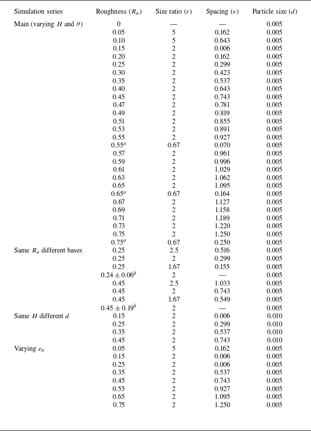
Base roughness specifications for various simulations series.

Notes:
 $^a$
Simulations with relatively large base particles (
 $r\lt 1$
), which show slightly different basal layer shear rate profiles in figure 4(b).
 $^b$
Simulations with randomly arranged base particles, where
 $R_a$
varies in a range quantified by the standard deviation of the void area.
For a given
 $r$
, it is required that
 $\epsilon \leqslant (\sqrt {3}/2)(1+r) - 1$
, such that
 $R_a \leqslant 1$
. Physically, this condition indicates that, if the triangular voids formed by the base particles are too large, flowing particles can percolate through or fill the voids, leading to a so-called void-filling mechanism and thereby reducing the apparent base roughness (Goujon et al. Reference Goujon, Thomas and Dalloz-Dubrujeaud2003; Jing et al. Reference Jing, Kwok, Leung and Sobral2016). Here, to avoid such complications for
 $R_a \rightarrow 1$
, we carefully choose
 $r$
and
 $\epsilon$
to restrict the range of
 $R_a$
from
 $0$
to
 $0.85$
, where
 $R_a = 0$
means a flat base without base particles. We also conduct simulations with the same
 $R_a$
but different combinations of
 $r$
and
 $\epsilon$
(including regular and random arrangements of base particles) to demonstrate the relevance of using
 $R_a$
as a single indicator of the geometric roughness (see Appendix A). Detailed base configurations for various simulation series are listed in table 1.
2.3. Steady flow conditions and mean flow fields
To allow a granular flow to reach steady state, it is helpful to first determine the
 $h_{\textit{stop}} (\theta )$
curve in the (
 $H$
,
 $\theta$
) parameter space, which is a curve delimiting no-flow (below the curve) and steady flow conditions (Pouliquen Reference Pouliquen1999). The
 $h_{\textit{stop}} (\theta )$
curve is usually measured using a sufficiently rough base, as lower base roughness can significantly affect
 $h_{\textit{stop}} (\theta )$
(Weinhart et al. Reference Weinhart, Thornton, Luding and Bokhove2012). In this study, the simulation protocol to determine
 $h_{\textit{stop}} (\theta )$
is as follows. For a given
 $R_a$
and
 $H$
, we initiate the granular flow at a certain slope angle and then decrease stepwise the slope angle at an increment of
 $0.1^\circ$
, holding for a sufficient period to check the flow state (accelerating, steady or decelerating to stop). Such a slope-reducing procedure continues until the system kinetic energy visually vanishes, at which the current slope angle is marked as
 $\theta _{\textit{stop}}$
and the corresponding flow thickness (measured as twice the
 $z$
-centre of mass for all particles) is marked as
 $h_{\textit{stop}}$
.
Following this protocol, we conduct simulations to measure
 $h_{\textit{stop}}(\theta )$
for
 $R_a$
varying from
 $0.01$
to
 $0.85$
, as shown in figure 2(a). Interestingly, the
 $h_{\textit{stop}}(\theta )$
curve is nearly vertical for small
 $R_a$
, corresponding to a Coulomb friction-like condition (Artoni et al. Reference Artoni, Santomaso, Go and Canu2012), and is shifted significantly to the right as
 $R_a$
is increased. For sufficiently rough bases (
 $R_a\gt 0.6$
), the
 $h_{\textit{stop}}(\theta )$
curves converge to a master curve that is similar to those reported in previous studies (Pouliquen Reference Pouliquen1999; Weinhart et al. Reference Weinhart, Thornton, Luding and Bokhove2012). The master curve of
 $h_{\textit{stop}}(\theta )$
is fitted to the following expression:
 \begin{equation} \frac {h_{\textit{stop}}}{d} = A\frac {\tan {\theta _2} - \tan {\theta }}{\tan {\theta } - \tan {\theta _1}}. \end{equation}
Here
 $A=1.45$
,
 $\theta _1=19.56^\circ$
and
 $\theta _2=37.24^\circ$
are fitting coefficients, which depend primarily on material properties as long as the base is sufficiently rough (Pouliquen Reference Pouliquen1999; Liu et al. Reference Liu, Jing, Pähtz, Cui, Zhou and Fu2024). These fitting parameters are quantitatively similar to previous DEM simulations of spheres (Liu et al. Reference Liu, Jing, Pähtz, Cui, Zhou and Fu2024). Finally, we show in figure 2(b) that our main simulations (marked by cross symbols) are chosen in the steady flow region well above the master curve of
 $h_{\textit{stop}} (\theta )$
.
(a) Results of the
 $h_{\textit{stop}}$
curves for
 $R_a$
varying from
 $0.01$
to
 $0.85$
. (b) The master
 $h_{\textit{stop}}$
curve for sufficiently rough bases (
 $R_a\gt 0.6$
) and the main simulation conditions (
 $\theta ,H/d$
) for steady-state flows.

Once a simulation reaches steady state (when the system kinetic energy does not vary in time), we compute various time-averaged mean flow fields based on the DEM data (following the formulations of Silbert et al. Reference Silbert, Ertaş, Grest, Halsey, Levine and Plimpton2001) in a series of
 $1d$
-thick layers, including the volume fraction
 $\phi$
, streamwise velocity
 $u$
, shear rate
 $\dot {\gamma } = \partial u / \partial z$
, granular temperature
 $T = (u_p - u)^2$
, where
 $u_p$
is the instantaneous particle velocity, pressure (or normal stress)
 $P = \sigma _{zz}$
, shear stress
 $\tau = \sigma _{xz}$
, effective friction
 $\mu = \tau /P$
and inertial number
 $I = \dot {\gamma }d / \sqrt {P/\rho _p}$
. All quantities are functions of the
 $z$
position, with
 $z=0.5d$
denoting the position of the lowermost data point. Note that a correction for the granular temperature with velocity gradients has been proposed by Artoni & Richard (Reference Artoni and Richard2015
a) to account for the dependence of the computed velocity fluctuation on the averaging domain size. This does not significantly affect our results and conclusions, but might warrant more quantitative investigations in future work.
3. Flow kinematics
3.1. Kinematics features of basal layer for varying base roughness
Figure 3 presents steady-state snapshots of the granular flow simulations for varying
 $R_a$
with a fixed set of flow conditions (
 $H/d=40$
and
 $\theta =25^\circ$
), where the particles are coloured by layerwise values of the inertial number
 $I$
. For an example case of
 $R_a=0.15$
(figures 3
a and 3
b), which is relatively smooth, three layers of the flow can be identified: a dilated basal layer, a dense bulk layer (also known as the core), and a saltating surface layer. Although the three-layer structure is typical of steady-state flows down a bumpy base (Louge Reference Louge2003), it is clear from figure 3(c) that
 $R_a$
controls the formation of the basal layer. A geometrically smoother plane leads to a basal layer that is much more dilated and energetic, with values of
 $I$
well above the typical value of
 $I\lt 1$
for dense granular flows. Such basal layer behaviours have previously been noted as density inversion or the supported regime (Taberlet et al. Reference Taberlet, Richard, Jenkins and Delannay2007; Brodu et al. Reference Brodu, Delannay, Valance and Richard2015), which can be understood as heating (i.e. increase of granular temperature) due to effective velocity slip of the basal layer particles along the bottom plane (Hui et al. Reference Hui, Haff, Ungar and Jackson1984; Richman Reference Richman1988; Kumaran Reference Kumaran2008).
Typical three-layer structure of inclined granular flows. Panels (a) and (b) are an example case of
 $R_a=0.15$
. (c) Basal layer for smooth (
 $R_a=0.05$
) to rough (
 $R_a=0.75$
) planes. All 2-D snapshots are captured from three-dimensional (3-D) simulations at steady state, with particles coloured by the local inertial number
 $I$
.

Results for varying
 $R_a=0.05{-}0.75$
with fixed
 $H/d=40$
and
 $\theta =25^\circ$
in terms of (a) velocity, (b) shear rate, (c) granular temperature, (d) volume fraction, and (e) the correlation between granular temperature and shear rate in both bulk and basal layers. The open circles denote the DEM results with their colour indicating
 $R_a$
, while the dashed and solid curves in (a–c) are fittings based on models (3.1) and (3.3), respectively.

To quantify the effects of
 $R_a$
on the kinematics features of the flow, we show flow-depth profiles of dimensionless velocity
 $u/\sqrt {\textit{gd}}$
, shear rate
 $\dot {\gamma }/\sqrt {g/d}$
and granular temperature
 $T/\sqrt {\textit{gd}}$
, as well as the volume fraction
 $\phi$
, in figure 4, with
 $R_a$
varying from
 $0.05$
to
 $0.75$
at an increment of
 $0.1$
(
 $H/d=40$
and
 $\theta =25^\circ$
). Figure 4(a) shows that a typical Bagnold velocity profile passing through the origin (no slip) is observed for
 $R_a\geqslant 0.55$
, but the profile is sequentially shifted to the right as
 $R_a$
becomes smaller (from blue to red symbols), indicating an increase in the basal slip velocity. The velocity profiles for all
 $R_a$
are parallel to Bagnold’s profile in the bulk, but a longer tail near the base is observed for lower-
 $R_a$
cases. Based on these observations, we use the following modified Bagnold velocity profile (dashed curves) to fit the simulation data (symbols):
 \begin{equation} \frac {u_{\textit {Bag}1}}{\sqrt {\textit{gd}}} = \frac {u_{b1}}{\sqrt {\textit{gd}}} + \frac {2}{3}\bar {I}\sqrt {\bar \phi \cos {\theta }} \left [ \left (\frac {h}{d}\right )^{3/2} - \left (\frac {h-z}{d}\right )^{3/2} \right ]\!. \end{equation}
Here
 $u_{b1}$
is a fitting parameter representing an effective slip velocity (see Appendix B for a detailed derivation of the expression). Note that the flow thickness
 $h$
is defined by the
 $z$
coordinate of the uppermost data point and we use the bulk-averaged inertial number
 $\bar {I}$
and volume fraction
 $\bar \phi$
of each case for fitting. The basal layer thickness can be roughly considered as where the velocity data deviates from the dashed curve (manually marked by red filled circles), which seems to be insensitive to
 $R_a$
(see § 3.5 for more discussions). Moreover, in Appendix A we present results of the same
 $R_a$
but different base particle arrangements, verifying that the use of
 $R_a$
as a single roughness indicator is reasonable.
The parallelness of the bulk velocity profiles in figure 4(a) is more evident in figure 4(b), where the shear rate profiles for all
 $R_a$
(symbols) overlap in the bulk region, following Bagnold’s shear rate profile (dashed curve), but deviate systematically in the basal layer. Specifically, a smaller
 $R_a$
corresponds to higher shear rates in the basal layer (from blue to red), reflecting the longer tails of the velocity profiles in figure 4(a). Similar trends are found in figure 4(c) for the granular temperature profiles, where the basal layer for low values of
 $R_a$
is significantly heated (and hence dilated as shown in figure 3). The dilated basal layer is also evident in the volume fraction profiles, figure 4(d), where the bulk values of
 $\phi$
are constant. Finally, we note that the similarity of the temperature and shear rate profiles is expected, because the following relation has been widely reported in steady granular flows (da Cruz et al. Reference da Cruz, Emam, Prochnow, Roux and Chevoir2005; Kim & Kamrin Reference Kim and Kamrin2020; Rognon & Macaulay Reference Rognon and Macaulay2021):
 \begin{equation} \sqrt {T} = \alpha \dot {\gamma } d. \end{equation}
Here
 $\alpha = 0.72$
is a proportionality constant according to our simulation data, from both bulk and basal layers, as shown in figure 4(e). This correlation is used to derive the temperature profiles in figure 4(c) (dashed curves); see also Appendix B.
Now that the relations between velocity, shear rate and temperature are clear, it is possible to provide a more accurate functional form for the velocity profiles in figure 4(a) and therefrom derive the shear rate (figure 4 b) and temperature profiles (figure 4 c). We propose a general expression for the velocity profile considering the detailed shape of the basal layer (solid curves in figure 4 a):
 \begin{equation} \frac {u_{\textit {Bag}2}}{\sqrt {\textit{gd}}} = \frac {u_{b2}}{\sqrt {\textit{gd}}} +\frac {\Delta u}{\sqrt {\textit{gd}}}\left [1-\exp \left (-\frac {z}{z_c}\right ) \right ] + \frac {2}{3}\bar {I}\sqrt {\bar \phi \cos {\theta }} \left [ \left (\frac {h}{d}\right )^{3/2} - \left (\frac {h-z}{d}\right )^{3/2} \right ]\!. \end{equation}
Here
 $u_{b2}$
,
 $\Delta u$
and
 $z_c$
are fitting parameters with clear physical meanings. Specifically,
 $u_{b2} = u(z = 0)$
is the (fitted) true basal slip velocity,
 $\Delta u$
represents the difference between the true and effective slip velocities (i.e.
 $\Delta u=u_{b1}-u_{b2}$
), and
 $z_c$
is a characteristic distance for the basal slip velocity to change towards the bulk. Note that the assumed exponential decay function makes it convenient to define the basal layer thickness
 $h_b = 3z_c$
, corresponding to where the difference between the flow velocity and Bagnold’s profile drops to about 5 % (figure 4
a). This definition of
 $h_b$
is found to be robust for most simulation conditions in this work, which is used and discussed in § 3.5. Note also that (3.3) can be easily converted into equations for shear rate (derivative in
 $z$
) and temperature profiles (using (3.2)), where the exponential function captures the decay of slip-generated shear rates and temperatures in the basal layer, as shown in figure 4(b) and 4(c) (solid curves).
3.2. Effects of slope angle and flow thickness
To this point, we have investigated the basal effects with fixed slope angle
 $\theta$
and initial flow thickness
 $H$
. Figure 5(a) shows the effects of varying
 $\theta$
from
 $23^\circ$
to
 $27^\circ$
with
 $H/d=40$
for a relatively smooth base (
 $R_a=0.25$
). Both mean velocity and slip velocity increase significantly as
 $\theta$
is increased (blue to red data points). The velocity profiles can again be well described by (3.1) and (3.3), see black dashed and red solid curves, respectively, indicating that the bulk velocity follows Bagnold’s scaling. The exponential tail in the basal layer seems to vary its shape as
 $\theta$
is varied, which is a rather non-trivial dependence; we address the detailed scaling of basal slip velocity in § 3.3. Nevertheless, figure 5(b) shows that if one shifts the velocity profile to the origin, i.e.
 $u(z)-u_{b1}$
, where
 $u_{b1}$
is obtained using (3.1), all velocity profiles for varying
 $R_a$
fall on branches defined only by
 $\theta$
. In other words, the boundary effect decays rapidly within a few particles distance and has negligible influence beyond. Bulk particles can be viewed as a flow running atop the fast-moving basal layer, and the internal deformation rate within the bulk is determined by Bagnold’s scaling or the local rheology (i.e. the shear stress scales with the square of the shear rate).
(a) Velocity profiles for varying
 $\theta =23^\circ{-}28^\circ$
with fixed
 $H/d=40$
and
 $R_a=0.25$
. (b) Shifted velocity profiles for varying
 $\theta$
and
 $R_a$
with fixed
 $H/d=40$
. (c) Velocity profiles for varying
 $H/d=20{-}60$
with fixed
 $\theta =25^\circ$
and
 $R_a=0.25$
. (d) Volume fraction profiles for varying
 $H/d=20{-}60$
or
 $\theta =23^\circ{-}27^\circ$
, with fixed
 $R_a=0.25$
. (e) Correlation between
 $T/gd$
and
 $\dot \gamma d$
in the basal layer for varying
 $R_a$
,
 $H/d$
and
 $\theta$
, which follows (3.2). The open circles in (a–c) denote DEM results, while the dashed and solid curves are fits to (3.1) and (3.3), respectively.

In figure 5(c) we show velocity profiles for varying
 $H/d$
with a fixed slope (
 $\theta =25^\circ$
) and smooth base (
 $R_a=0.25$
). Similarly, the bulk flow follows Bagnold’s scaling and the basal layer velocity profile depends somewhat on
 $H/d$
(see § 3.3). Intriguingly, the thickness of the basal layer, marked by red filled circles, does not grow with the overall flow thickness. This indicates that the basal layer is a local phenomenon determined by particle-scale interactions and that the excess energy (granular temperature) generated at the slippery bottom plane is dissipated via collisions in just a few particle layers. We address the scaling of the basal layer thickness in § 3.5.
Figure 5(d) shows typical profiles of volume fraction for varying
 $H/d$
or
 $\theta$
, which show consistent slip-induced dilatation in the basal layers. The constant
 $\phi$
values in the bulk are determined mainly by the slope angle but not the flow thickness. More systematic exploration of the scaling of
 $\phi$
is presented in § 4.
Profiles of shear rate and granular temperature for varying
 $\theta$
and
 $H/d$
are omitted as they are similar to those in figure 4. Rather, figure 5(e) shows the correlation
 $\sqrt {T} \propto \dot {\gamma }d$
, consistent with (3.2), for all basal layer datasets with varying
 $R_a=0{-}0.55$
,
 $\theta =23^\circ{-}27^\circ$
and
 $H/d=20{-}60$
. This correlation further verifies that the velocity, shear rate and temperature profiles can be empirically described using (3.3), its
 $z$
derivative and (3.2) for all conditions studied here. Of course, it is also interesting to derive alternative theoretical descriptions of the kinematics profiles using kinetic theory of granular flow (Kumaran Reference Kumaran2008; Berzi Reference Berzi2024), as further discussed in § 4, but this is beyond the scope of this work.
3.3. Scaling of basal slip velocity: Navier slip formulation
Predicting the basal slip velocity is key to describing granular flows down an insufficiently rough incline. The empirical models (3.1) and (3.3) can only be used if the fitted value of
 $u_{b1}$
or
 $u_{b2}$
is known. To investigate how the slip velocity depends on various simulation conditions (
 $R_a$
,
 $\theta$
and
 $H/d$
), we first plot
 $u_b/u_s$
vs
 $R_a$
for
 $\theta =23^\circ{-}27^\circ$
and
 $H/d=20{-}60$
in figure 6(a), where
 $u_b$
and
 $u_s$
are DEM averaged velocities at the lowermost (basal) and uppermost (surface) flow layers in a velocity profile, respectively, following Jing et al. (Reference Jing, Kwok, Leung and Sobral2016). Despite the spread of the data, it is clear that
 $u_b/u_s$
decreases from
 $0.6\pm 0.1$
towards zero, as
 $R_a$
is increased from
 $0$
to
 $0.6$
, and remains zero (no-slip) beyond the threshold value of
 $R_a^{cr}=0.6$
. Such slip-to-no-slip transition is consistent with previous DEM simulations in Jing et al. (Reference Jing, Kwok, Leung and Sobral2016), as marked by vertical dashed lines in figure 6(a).
Scaling of slip velocity. Main simulation results of (a)
 $u_b/u_s$
and (b)
 $l_s=u_b/\dot \gamma d$
vs
 $R_a$
for various flow conditions (
 $\theta$
and
 $H/d$
). (c) The flat-base slip length
 $l_s^0$
vs
 $\tan \theta /\mu _{pw}$
from our simulations (filled symbols and solid curve) and previous work (Artoni et al. Reference Artoni, Santomaso, Go and Canu2012) (open symbols and the corresponding curves). The curves are fits to (3.5). (d) All results of
 $l_s$
vs
 $l_s^0(1-R_a/R_a^{cr})$
for varying
 $R_a$
,
 $\theta$
and
 $H/d$
. Coloured symbols represent the same cases as (a) and (b). The added symbols are additional simulations with different base configurations and particle sizes (
 $H/d=40$
and
 $\theta =23^\circ$
).

Although basal slip appears to be controlled by
 $R_a$
, the data scatter in figure 6(a) suggests that
 $\theta$
and
 $H/d$
can also affect the results. However, there is no straightforward way to express
 $u_b/u_s$
as a function of
 $\theta$
and
 $H/d$
. In figure 6(b) we rescale
 $u_b$
as
 $l_s=u_b/\dot \gamma _b d$
following a Navier slip velocity formulation proposed by Artoni et al. (Reference Artoni, Santomaso, Go and Canu2012), where
 $l_s$
is called the slip length and
 $\dot \gamma _b$
is the basal shear rate measured in the lowermost flow layer. In this way, we effectively remove the
 $H/d$
dependence and find a clear monotonic dependence of
 $u_b/\dot \gamma _b d$
vs
 $R_a$
on
 $\theta$
(from blue to red data,
 $\theta$
increases). For simplicity, we fit the data series for each
 $\theta$
in figure 6(b) by a straight line passing through
 $(R_a^{cr},0)$
, and the intersection of this line with the vertical axis is denoted as
 $l_s^0$
, meaning the slip length for a flat-base case (
 $R_a=0$
). Moreover, to consider the effects of
 $\theta$
, we exploit the fact that in steady-state inclined flows,
 $\mu =\tau /P=\tan \theta$
due to force balance (Silbert et al. Reference Silbert, Ertaş, Grest, Halsey, Levine and Plimpton2001), where
 $\mu$
is the effective friction of the flow. As such, we propose the following semi-empirical scaling law for the slip velocity:
 \begin{equation} \begin{cases} l_s:=\frac {u_b}{\dot \gamma _b d} = l_s^0 \left ( 1-\frac {R_a}{R_a^{cr}}\right )\!, & R_a\lesssim R_a^{cr},\\ u_b=0, & \rm {otherwise.} \end{cases} \end{equation}
Here
 $R_a^{cr}=0.6$
is an empirical threshold roughness below which slip occurs and
 $l_s^0$
is the flat-base slip length established by Artoni et al. (Reference Artoni, Santomaso, Go and Canu2012),
 \begin{equation} l_s^0:=\frac {u_b}{\dot \gamma _b d}\Big |_{R_a=0}=a\!\left ( \frac {\mu /\mu _{pw}}{c-\mu /\mu _{pw}}\right )^b\!, \end{equation}
where
 $a$
,
 $b$
and
 $c$
are fitting parameters, and
 $\mu _{pw}$
is the coefficient of friction between particles and the bottom wall, which mainly affects the results when geometric roughness (
 $R_a$
) is absent (Thornton et al. Reference Thornton, Weinhart, Luding and Bokhove2012; Jing et al. Reference Jing, Kwok, Leung and Sobral2016); here, we fix
 $\mu _{pw}=0.5$
. Fitting parameters
 $a$
,
 $b$
and
 $c$
are material dependent and, as shown in figure 6(c), we find that
 $a=2.09$
,
 $b=0.42$
and
 $c=1.05$
in our three-dimensional (3-D) simulations of spherical particles. Interestingly, these values are comparable to the 2-D simulation results reported by Artoni et al. (Reference Artoni, Santomaso, Go and Canu2012), i.e.
 $a=2.2$
,
 $b=0.42$
and
 $c=1$
for elongated polygons and
 $a=3.66$
(the reported value in Artoni et al. (Reference Artoni, Santomaso, Go and Canu2012) was
 $a=4.23$
, which does not match the data well),
 $b=0.33$
and
 $c=1$
for regular polygons, as also included in figure 6(c). Moreover, we find that flat-base simulations cannot reach steady state at slope angles close to the particle-wall contact friction angle (
 $\theta \rightarrow \tan ^{-1}\mu _{pw}$
), hence, the missing data points for
 $(\theta =27^\circ , R_a=0)$
in figure 6(b) and the diverging curves at
 $\tan \theta /\mu _{pw}\rightarrow 1$
in figure 6(c).
In figure 6(d) we plot
 $l_s$
vs
 $l_s^0(1-R_a/R_a^{cr})$
according to the scaling law (3.4) and (3.5), which collapses results for all simulation conditions (
 $R_a=0{-}0.75$
,
 $\theta =23^\circ{-}27^\circ$
and
 $H/d=20{-}60$
) onto a single curve. Moreover, figure 6(d) include two sets of additional simulations (black symbols): one with the same
 $R_a$
but different (
 $r$
,
 $\epsilon$
) to demonstrate the robustness of using
 $R_a$
as a unified roughness parameter (see also Appendix A), and another with the same
 $H$
but varying
 $d$
to confirm that the particle size is the correct length scale in
 $l_s$
. Detailed simulation parameters for the added cases are listed in table 1. Good agreement is found for all cases between the model predictions and simulation results, which validates our slip law as a generalisation of the flat-base slip law proposed by Artoni et al. (Reference Artoni, Santomaso, Go and Canu2012) accounting for the effects of geometric roughness.
3.4. Scaling of basal slip velocity: temperature-based formulation
An alternative slip law is to scale
 $u_b$
by the square root of the basal temperature,
 $\sqrt {T_b}$
, as found in previous DEM simulations (Artoni & Richard Reference Artoni and Richard2015b
; Breard et al. Reference Breard, Dufek, Fullard and Carrara2020; Richard et al. Reference Richard, Artoni, Valance and Delannay2020) and derived using kinetic theory of granular flows (Hui et al. Reference Hui, Haff, Ungar and Jackson1984; Richman Reference Richman1988; Jenkins Reference Jenkins2007; Berzi & Vescovi Reference Berzi and Vescovi2017; Gollin et al. Reference Gollin, Berzi and Bowman2017). Figure 7(a) presents rescaled results of
 $u_b/\sqrt {T_b}$
vs
 $R_a$
for all main simulations, which appears to collapse better than figure 6(b) in terms of the
 $\theta$
dependence. Similar 3-D DEM simulations of spheres on flat and rough inclined surfaces by Breard et al. (Reference Breard, Dufek, Fullard and Carrara2020) show similar results (although their results are systematically lower at medium values of
 $R_a$
), as reproduced in figure 7(a). Note that Breard et al. (Reference Breard, Dufek, Fullard and Carrara2020) used the roughness angle,
 $\sin \psi$
, which we convert to
 $R_a$
using the relation
 $R_a=(4/3)\sin ^2\psi$
(see § 2). Note also that Breard et al. (Reference Breard, Dufek, Fullard and Carrara2020) calculated the slip velocity by considering the mean velocity of all particles contacting the base, whereas we extract
 $u_b$
from the lowermost binning layer, which might be responsible for the differences in the results. Nevertheless, the agreement for
 $R_a=0$
is excellent, as shown in figure 7(b) and discussed shortly.
Granular temperature-based scaling of slip velocity. (a) Rescaled slip velocity
 $u_b/\sqrt {T_b}$
as a function of
 $R_a$
for varying
 $H/d$
and
 $\theta$
(same simulations as in figure 6. The curves are predictions of model (3.6); see text. The black triangles are polydisperse inclined flow simulation results of Breard et al. (Reference Breard, Dufek, Fullard and Carrara2020). (b) Rescaled effective friction
 $\mu _w/\mu _{pw}$
as a function of
 $u_b/\sqrt {T_b}$
for flat-wall simulations (
 $R_a=0$
), following three scaling laws from the literature (Jenkins Reference Jenkins1992; Artoni & Richard Reference Artoni and Richard2015b
; Breard et al. Reference Breard, Dufek, Fullard and Carrara2020). DEM simulation data of Breard et al. (Reference Breard, Dufek, Fullard and Carrara2020) are also included.

The relation between
 $u_b/\sqrt {T_b}$
and base roughness has been derived as a boundary condition in the granular kinetic theory (Richman Reference Richman1988; Gollin et al. Reference Gollin, Berzi and Bowman2017),
 \begin{equation} \frac {u_b}{\sqrt {T_b}}=\left (\frac {\pi }{2}\right )^{1/2}\mu _b \left [\frac {1}{3\sqrt {2}J_b}\frac {2^{3/2}J_b-5F_b(1+B_b)\sin ^2\psi }{2(1-\cos \psi )/\sin ^2\psi -\cos \psi }+\frac {5F_b}{2^{1/2}J_b}\right ], \end{equation}
where
 $B=\pi [1+5/(8\phi g_0)]/(12\sqrt {2})$
,
 $F=(1+e_n)/2+1/(4\phi g_0)$
,
 $J$
and
 $g_0$
are given in Appendix C, and the subscript
 $b$
denotes variables computed at the base (lowermost layer of our binning results). For simplicity, we take
 $\mu _b=\tan \theta$
and
 $\phi _b$
to be a constant for each
 $R_a$
and
 $\theta$
, although both can vary in the basal layer (see § 4); we verify that considering the variations in
 $\phi _b$
does not change the model prediction significantly. The predictions of (3.6) for various
 $\theta$
are plotted in figure 7(a), where we convert
 $\sin \psi$
and
 $\cos \psi$
to
 $R_a$
using
 $R_a=(4/3)\sin ^2\psi$
and
 $\sin ^2\psi +\cos ^2\psi =1$
. While the predictions do not precisely capture our DEM results for each
 $\theta$
(indicated by colours) and they diverge at
 $R_a\rightarrow 0$
, the overall agreement is decent. This motivates further improvement of the boundary condition for kinetic theory.
For flat walls (
 $R_a=0)$
, DEM-based scaling relations between
 $u_b/\sqrt {T_b}$
and
 $\mu _w/\mu _{pw}$
have been established in inclined and wall-confined flows (Artoni & Richard Reference Artoni and Richard2015b
; Breard et al. Reference Breard, Dufek, Fullard and Carrara2020; Richard et al. Reference Richard, Artoni, Valance and Delannay2020), where
 $\mu _w$
is the effective friction measured at the lateral or bottom wall. Figure 7(b) shows the comparison of our data and previous models. While the empirical model of Artoni & Richard (Reference Artoni and Richard2015b
) (dashed curve) predicts smaller
 $u_b/\sqrt {T_b}$
in general for wall-confined flows (where creeping occurs easily), the inclined flow results of Breard et al. (Reference Breard, Dufek, Fullard and Carrara2020) agree with our results very well (red and blue for mono- and polydisperse flows, respectively). We follow the empirical model of Breard et al. (Reference Breard, Dufek, Fullard and Carrara2020) to fit the data,
 \begin{equation} \mu _w=a+\frac {\mu _{pw}-a}{1+b(u_b/\sqrt {T_b})^c}, \end{equation}
where
 $a$
,
 $b$
and
 $c$
are empirical fitting coefficients. Specifically, for monodisperse flows,
 $a=0.283$
,
 $b=27\,178$
and
 $c=5.22$
, whereas for polydisperse flows,
 $a=0.296$
,
 $b=55\,783$
and
 $c=5.71$
. Note that our data are concentrated at the higher end of the curves, because the slope angles we explore are well above the angle of repose of the material (see § 2).
Dependence of basal layer thickness
 $h_b/d$
on (a) the base roughness
 $R_a$
(
 $H/d=20, 40, 60$
;
 $\theta =23^\circ{-}27^\circ$
) and (b) the coefficient of restitution
 $e_n$
(
 $H/d=40$
,
 $\theta =25^\circ$
). Error bars in (a) indicate uncertainties of obtaining
 $h_b=3z_c$
via fitting the velocity profiles to model (3.3), where
 $z_c$
is a fitting parameter. The crosses in (a) represent the rough-base cases (
 $R_a=0.55$
,
 $0.65$
and
 $0.75$
) where the base particles are larger than the flow particles (
 $r=0.67$
). The solid curve in (b) is a fit to
 $h_b/d=\beta /\sqrt {1-e_n}$
according to Kumaran (Reference Kumaran2008); see text.

Finally, various slip boundary conditions for flat walls can also be found in the granular kinetic theory. Here, we test the piecewise linear approximation proposed by Jenkins (Reference Jenkins1992), which predicts that
 ${\mu _w/\mu _{pw}}\propto {u_b/\sqrt {T_b}}$
, with a proportionality constant of
 $\sqrt {3}/(2{\overline {\mu }_0})$
, for small slip velocities, i.e.
 $u_b/\sqrt {T_b}\leqslant {(2\sqrt {3}/3)}\overline {\mu }_0$
; and
 ${\mu _w/\mu _{pw}}=1$
, for otherwise larger slip velocities. Here,
 $\overline {\mu }_0=\mu _{pw}(7/2)(1+e_n)/(1+e_t)$
is a constant, and we have
 $\overline {\mu }_0=7/4$
as we use
 $\mu _{pw}=0.5$
and the tangential coefficient restitution
 $e_t=e_n=0.8$
in this study. The piecewise linear relation is plotted in figure 7(b) as a black solid curve, which generally captures the trend but does not match our DEM data; similar observations are made by Berzi, Jenkins & Richard (Reference Berzi, Jenkins and Richard2020). Note that the slip velocity defined by Jenkins (Reference Jenkins1992) includes the rotational contribution, which is not considered in the present work and other cited work (Artoni & Richard Reference Artoni and Richard2015b
; Breard et al. Reference Breard, Dufek, Fullard and Carrara2020). Note also that adopting a more precise solution of Jenkins (Reference Jenkins1992) does not match the DEM results either, which is therefore omitted for brevity. In short, while empirical models are provided for the granular temperature-based slip law, more research is needed in the future to develop more predictive and accurate kinetic theory-based boundary conditions.
3.5. Scaling of basal layer thickness
An intriguing observation in figures 4 and 5 is that the basal layer thickness
 $h_b$
is generally insensitive to all simulation conditions (
 $R_a$
,
 $\theta$
,
 $H/d$
). To investigate this, we plot
 $h_b/d$
vs
 $R_a$
for varying
 $\theta =23^\circ{-}27^\circ$
and
 $H/d=20{-}60$
in figure 8(a). Despite the scatter, partly due to difficulties in consistently defining
 $h_b$
(we use
 $h_b=3z_c$
, where
 $z_c$
is a fitting parameter; see § 3.1), it is evident that the basal layer thickness is only a few particle diameters even for significantly increased
 $H/d$
. More specifically, for
 $R_a \lesssim 0.45$
(slip regime),
 $h_b\approx 3d$
is nearly a constant except for the
 $\theta =27^\circ$
cases (red symbols). For the transitional (
 $0.45 \lesssim R_a \lesssim 0.6$
) and no-slip regimes (
 $R_a \gtrsim 0.6$
), the scatter of the data increases, likely because
 $h_b=3z_c$
depends somewhat on the goodness of fitting (error bars) when expression (3.3) is used to fit the velocity profiles (figures 4 and 5). For rough bases (
 $R_a \gtrsim 0.6$
), the assumption of an exponential tail in expression (3.3) may not hold, especially for
 $r\lt 1$
cases where the shear rate in the basal layer points to zero due to the geometric constrains of the roughness (see figure 4
b), hence, greater uncertainties in the results (crosses in figure 8
a). Nevertheless, it is interesting that a basal layer, where the velocity deviates from Bagnold’s, occurs even for the no-slip regime and the basal layer thickness is not wildly different from the slip regime. The systematic
 $\theta$
dependence of
 $h_b$
in the no-slip regime (
 $R_a \gtrsim 0.6$
) is somewhat consistent with a previous study (Thornton et al. Reference Thornton, Weinhart, Ogarko and Luding2013).
The observation that
 $h_b$
does not grow with
 $H$
indicates that the basal layer dynamics is mainly controlled by particle-scale mechanisms. In kinetic theory of granular flows, this can be understood as the balance of fluctuation kinetic energy among three terms: energy generation due to shear work, conduction along the temperature gradient and dissipation due to inelastic collisions. Following this idea, Kumaran (Reference Kumaran2008) derived an expression for a conduction length,
 $\delta =d/\sqrt {1-e_n}$
, near the base of an inclined granular flow, which is the length over which the rate of energy conduction is comparable to the rate of collisional dissipation. Interestingly,
 $\delta /d$
does not depend on flow conditions, as observed here, but is dependent on the material property
 $e_n$
. To confirm the relevance of this scaling, we run additional simulations with varying
 $e_n=0.1{-}0.9$
and
 $R_a=0.05{-}0.75$
for fixed
 $\theta =25^\circ$
and
 $H/d=40$
. As shown in figure 8(b), the scaling
 $h_b/d=\beta /\sqrt {1-e_n}$
agrees reasonably with our data for the slip regime,
 $R_a\leqslant 0.45$
, where
 $\beta =1.42$
is a fitting parameter. The slight disagreement may be attributed to the simplification of the conduction length derivation where particle friction was not considered, as noted by Kumaran (Reference Kumaran2008).
4. Rheology
In the preceding section we showed that granular flows down an insufficiently rough plane (
 $R_a\lesssim 0.6$
) can exhibit a dilute, highly agitated basal layer beneath the dense bulk, where the kinematics profiles (velocity, shear rate and granular temperature) deviate from Bagnold’s profiles or from what the local
 $\mu (I)$
rheology can predict. Next, we explore friction (or stress) and volume fraction data in the basal and bulk layers to further understand the basal layer dynamics from a rheological point of view (figure 9).
Rheological and stress results. Solid (bulk) and open (basal) symbols are results of DEM simulations, whereas curves are predictions of empirical models or the granular kinetic theory. In (c–f) the solid curves are predictions of the rigid-sphere kinetic theory models, while the dashed curves are based on models where an estimated lower-bound particle stiffness is considered; see text and Appendix C for details.

Figures 9(a) and 9(b) show
 $\mu (I)$
and
 $\phi (I)$
graphs to test the local rheology established in dense granular flow studies (Jop et al. Reference Jop, Forterre and Pouliquen2006; Forterre & Pouliquen Reference Forterre and Pouliquen2008). Here, filled and open symbols are data from the bulk and basal layers, respectively, while symbol shapes and colours indicate the simulation conditions (
 $H/d$
,
 $\theta$
). Clearly, the bulk friction data (filled symbols in figure 9
a) follow the standard local rheology (solid curve),
 \begin{equation} \mu = \mu _s + \frac {\mu _{\infty } - \mu _s}{\left (I_0/I + 1\right )}, \end{equation}
where
 $\mu _s=0.36$
,
 $\mu _{\infty }=0.98$
and
 $I_0=0.90$
are fitting coefficients based on the bulk data. However, the data obtained from the basal layers (open symbols in figure 9
a) deviate significantly from the standard
 $\mu (I)$
curve. For a given
 $\theta$
(a given colour), while the values of
 $\mu$
are more or less constant due to force balance, i.e.
 $\mu =\tan \theta$
, the
 $I$
values can increase well beyond
 $1$
, reflecting the high shear rates near the bottom plane due to basal slip (§ 3). In other words, the one-to-one relation between
 $\mu$
and
 $I$
(i.e. local rheology) breaks down in the basal layer.
Likewise, the volume fraction results from the bulk (filled symbols in figure 9 b and inset) follow the standard local rheology (solid curve),
 \begin{equation} \phi = \phi _c - \kappa I, \end{equation}
where
 $\phi _c=0.58$
is the critical (maximum) volume fraction in the quasi-static limit (
 $I \rightarrow 0$
) and
 $\kappa =0.14$
is a fitting parameter. Data from the basal layers (open symbols in figure 9
b) deviate from this linear approximation, but they fall on a nonlinear master curve. That is, the low values of
 $\phi$
in the dilated basal layers can be roughly captured by the high values of
 $I$
(which encodes the effects of shear rate and pressure). It is possible to model this
 $\phi$
-
 $I$
relation using a cubic function, empirically,
 \begin{equation} \phi = \frac {\phi _c}{(\kappa 'I+1)^3}, \end{equation}
where
 $\kappa '=0.13$
is a fitting parameter. Model (4.3) can be viewed as a generalisation of the linear
 $\phi (I)$
model (4.2) towards the dilute, high-inertial-number limit.
Since the local rheology (4.1) does not hold in the basal layer, we seek alternative models for the granular stresses. Recently, Berzi (Reference Berzi2024) showed that Bagnold’s rheology and the granular kinetic theory can both capture the stresses (pressure and shear stress) in terms of shear rate, temperature and packing fraction for a wide range of dilute to dense flow configurations, encompassing inertial numbers from
 $10^{-3}$
to
 ${\sim}2$
. In figure 9(c) and 9(d) we follow Bagnold’s stress scaling to plot
 $P/(\rho _p d^2 \dot \gamma ^2)$
and
 $\tau /(\rho _p d^2 \dot \gamma ^2)$
as functions of
 $\phi$
, respectively. All data points from both the bulk and basal layers collapse on a master curve in each plot. Moreover, these data are captured by the Bagnold-like stress formulation suggested by Berzi (Reference Berzi2024) (solid curves; see Appendix C for derivation),
 \begin{align}&\,\, p=\frac {2J\phi [1+2(1+e_n)\phi g_0]}{15(1-e_{\textit{eff}}^2)}\left [1+\frac {26(1-e_{\textit{eff}})}{15}\frac {\mathcal{H}(\phi -0.49)(\phi -0.49)}{0.64-\phi }\right ]\rho _pd^2\dot {\gamma }^2, \end{align}
 \begin{align}& \tau =\frac {8J\phi ^2g_0}{5\pi ^{1/2}}\left [\frac {2J}{15(1-e_{\textit{eff}}^2)}\right ]^{1/2}\left [1+\frac {26(1-e_{\textit{eff}})}{15}\frac {\mathcal{H}(\phi -0.49)(\phi -0.49)}{0.64-\phi }\right ]\rho _pd^2\dot {\gamma }^2, \end{align}
where the expressions for the radial distribution function
 $g_0$
and dimensionless term
 $J$
are provided in Appendix C, the effective coefficient of restitution
 $e_{\textit{eff}}=e_n-(\pi /2)\mu _p+(9/2)\mu _p^2$
is derived for nearly elastic spheres and
 $\mathcal{H}(\boldsymbol{\cdot })$
is the Heaviside function. Note that the only parameters in (4.4) and (4.5) are
 $e_n=0.8$
and
 $e_{\textit{eff}}=0.63$
according to our model input (§ 2).
Lastly, we plot
 $P/(\rho _pT)$
and
 $\tau /(\rho _p dT^{1/2}\dot {\gamma })$
as functions of
 $\phi$
, respectively, in figures 9(e) and 9(f), following the kinetic theory stress models suggested by Berzi (Reference Berzi2024); see Appendix C. Again, all data points fall onto a single master curve in each plot, indicating the potential applicability of kinetic theory in describing the basal layer dynamics. The detailed dependence of these dimensionless stresses on the packing fraction (solid curves), derived for granular gases of frictional particles (Berzi Reference Berzi2024), is given by
 \begin{align} p & =\phi [1+2(1+e_n)\phi g_0]\rho _pT, \end{align}
 \begin{align}\tau & =\frac {8J\phi ^2g_0}{5\pi ^{1/2}}\rho _p d T^{1/2}\dot {\gamma }. \end{align}
Models (4.6) and (4.7) capture the main feature of the data in figure 9(e) and 9(f), but discrepancies are observed between the predictions (solid curves) and DEM results. This mismatch may be attributed to kinetic theory assumptions such as the single-particle velocity distribution function (Berzi Reference Berzi2024). Another plausible explanation for the mismatch is the lacking consideration of particle deformation in the stress formulation above (which considers rigid particles), especially when
 $\phi$
exceeds a critical value. To test this, we plot in figure 9(e) the model prediction (dashed curve) of scaled pressure for deformable, inelastic spheres, following Berzi & Jenkins (Reference Berzi and Jenkins2015), for an estimated finite particle stiffness; for details, see the final part of Appendix C. Similar tests are also conducted for other plots (dashed curves), but note that the model predictions are only for reference as they are based on simple shear assumptions; see Berzi et al. (Reference Berzi, Jenkins and Richard2020) for more discussion of inclined flow as a boundary-value problem. Nevertheless, the overall success of these kinetic theory models reinforces that the basal layer dynamics is controlled by the fluctuation kinetic energy, which is generated by shear work due to slip at the base and dissipated primarily due to inelastic collisions. Future work is expected to extend kinetic theory models (Richman Reference Richman1988; Kumaran Reference Kumaran2008; Gollin et al. Reference Gollin, Berzi and Bowman2017; Berzi et al. Reference Berzi, Jenkins and Richard2020) to predict the entire kinematics and rheological profiles in the basal layer as a boundary-value problem for all flow conditions explored here.
5. Conclusions
It has been long noticed that granular flows down an inclined plane can develop a dilute, highly agitated basal layer beneath the bulk, where the flow kinematics deviate from standard Bagnold’s profiles and where local rheology breaks down. However, a full picture of the basal layer dynamics remains unclear. Here, we use extensive DEM simulations of granular flows down smooth to rough inclines, with various flow conditions, to provide insights into the formation, kinematics, rheology and the associated scaling laws of the basal layer.
We find that the formation of a dilated basal layer is primarily controlled by the base roughness. As the roughness
 $R_a$
is varied from zero (flat base) to
 $0.75$
(sufficiently rough), three regimes are identified: a slip regime for smooth bases (
 $R_a\lesssim 0.45$
) where a dilated basal layer of several particle diameters appears, an intermediate regime (
 $0.45 \lesssim R_a \lesssim 0.6$
) where slip-to-no-slip transition occurs, and a no-slip regime for rough bases (
 $R_a \gtrsim 0.6$
) where the basal layer is not easily visible but deviations from Bagnold’s profile still exist. These flow regimes are roughly consistent with the slip-to-no-slip transition found in Jing et al. (Reference Jing, Kwok, Leung and Sobral2016) and the threshold values of
 $R_a$
are insensitive to flow conditions (slope angle and flow thickness).
The kinematics profiles (velocity, shear rate and temperature) are examined. When slip occurs, the bulk velocity profile (which follows Bagnold’s scaling) is shifted by an effective slip velocity, and the basal layer velocity profile appears to be exponential. This feature corresponds to an exponential increase in the basal layer shear rate and granular temperature profiles. Based on these observations, we propose a generalised Bagnold-like velocity profile considering the slip velocity and the characteristic thickness of the basal layer. Furthermore, a Navier-like slip law is developed for all roughness and flow conditions, which can be viewed as an extension of a previous slip law for flat-base inclined flows (Artoni et al. Reference Artoni, Santomaso, Go and Canu2012). We also examine various granular temperature-based slip laws (Artoni & Richard Reference Artoni and Richard2015b ; Gollin et al. Reference Gollin, Berzi and Bowman2017; Breard et al. Reference Breard, Dufek, Fullard and Carrara2020), showing that a slip boundary condition in the granular kinetic theory (Gollin et al. Reference Gollin, Berzi and Bowman2017) can capture the overall trend of the results.
Rheological data (stress, friction and volume fraction) extracted from the basal layer are analysed in various frameworks, including the local
 $\mu (I)$
rheology, Bagnold’s stress scaling and kinetic theory-based stress models. It is found that local rheology breaks down in the dilute, collision-dominated basal layer, while kinetic theory models can well describe the pressure and shear stress as functions of shear rate, temperature and volume fraction. These results indicate that the balance of fluctuation kinetic energy controls the basal layer dynamics and invite future development of kinetic theory models to fully resolve the kinematics and rheological profiles of the basal layer of granular flows.
Finally, while we focus on dry granular flows consisting of spherical particles down a rigid substrate, more realistic or complicated situations involving the effects of particle shape, segregation, interstitial fluids and erodible substrates can be considered in the future. Dynamics of thin-layer granular flows on smooth and rough planes, where the boundary layer effects dominate over the bulk flow, along with its implications for seismic signal generation in geophysical flows (Arran et al. Reference Arran, Mangeney, De Rosny and Toussaint2024), is also an interesting future direction.
Acknowledgements
We would like to thank Yifei Duan, Gengchao Yang, Thomas Pähtz and Diego Berzi for helpful discussions. T. Wang acknowledges the financial support received as a visiting student at Tsinghua Shenzhen International Graduate School, Tsinghua University. The numerical simulations were conducted using the high-performance computer clusters (HPC) at The University of Hong Kong.
Funding
Supported by the National Natural Science Foundation of China (12472412), the Research Grants Council of Hong Kong (17205821, 17205222, 17200724) and the Open Research Fund Program of State Key Laboratory of Hydraulics and Mountain River Engineering (SKHL2218).
Declaration of interests
The authors report no conflict of interest.
Data availability statement
The data that support the findings of this study, as well as the open-source codes for reproducing the simulations, are available from the corresponding author upon reasonable request.
Appendix A. Results of same
 $R_a$
but different base particle arrangements

The base roughness for granular flow is difficult to define, as it depends on the flow-to-base-particle size ratio
 $r$
, base particle spacing
 $\epsilon$
and the specific spatial arrangement (regular or random) of the base particles. To demonstrate that
 $R_a$
is a good indicator of the base roughness, figure 10 presents results for the same
 $R_a$
but different combinations of
 $r$
and
 $\epsilon$
with a regular or random arrangement (
 $H/d=40, \theta =23^\circ$
). It shows that, although the geometric features of the base vary significantly (see right panels), the velocity profiles are nearly identical for
 $R_a=0.45$
(slip-to-no-slip transition regime) and are reasonably close for
 $R_a=0.25$
(slip regime). Only the randomly generated bases (where the void areas have a distribution, see § 2.2) seem to always induce smaller basal slip, perhaps because larger voids have a stronger influence on the slip velocity. Nevertheless, the difference in terms of the slip velocity is within the range of uncertainties (see figure 6
d of the main text). Therefore, although an alternative roughness indicator that better collapses the data for
 $R_a=0.25$
warrants further studies, the use of
 $R_a$
effectively unifies the influence of
 $r$
and
 $\epsilon$
, which are major parameters determining the base roughness (Jing et al. Reference Jing, Kwok, Leung and Sobral2016).
Velocity profiles for the same
 $R_a$
but different base particle arrangements (
 $H/d=40, \theta =23^\circ$
). Detailed base configuration parameters are listed in table 1.

Appendix B. Modified Bagnold’s profiles considering basal slip velocity
Here we present the derivation of Bagnold’s velocity profile with slip velocity, as well as the shear rate and temperature profiles, assuming that the entire flow obeys the
 $\mu (I)$
rheology. An alternative form of Bagnold’s velocity profile using the rheology
 $\tau \propto \rho _pd^2\dot \gamma ^2$
leads to the same basic scaling as below but different fitting constants (Silbert et al. Reference Silbert, Ertaş, Grest, Halsey, Levine and Plimpton2001).
For steady, fully developed flows down an incline of slope
 $\theta$
in the
 $xz$
plane, integrating the momentum balance equations along the
 $z$
direction leads to
 $\tau =\phi \rho _pg\sin \theta (h-z)$
and
 $P=\phi \rho _pg\cos \theta (h-z)$
, such that
 $\mu =\tau /P=\tan \theta$
is constant. According to the
 $\mu (I)$
local rheology (Forterre & Pouliquen Reference Forterre and Pouliquen2008), where
 $\mu$
and
 $\phi$
are functions of
 $I$
, the volume fraction
 $\phi$
and inertial number
 $I$
are also constant along
 $z$
.
By identifying that
 $I=\dot \gamma d/\sqrt {P/\rho _p}$
, the shear rate
 $\dot \gamma$
can be expressed as
 \begin{equation} \dot \gamma := \frac {\partial u}{\partial z} = \frac {I\sqrt {P/\rho _p}}{d} = \frac {I\sqrt {\phi g\cos \theta }}{d} \left (h-z\right )^{1/2}. \end{equation}
Assuming a basal slip velocity,
 $u(z=0)=u_b$
, and integrating (B1) along
 $z$
, we have
 \begin{equation} u = u_b+\frac {2I\sqrt {\phi g\cos \theta }}{3d}[h^{3/2} - (h-z)^{3/2}]. \end{equation}
Substituting the empirical correlation
 $\sqrt {T}=\alpha \dot \gamma d$
for steady granular flows into (B1), the granular temperature profile can be expressed as
 \begin{equation} T = \alpha ^2I^2\phi \rho _p g\cos \theta (h-z). \end{equation}
In the main text (§ 3),
 $\phi$
and
 $I$
are obtained as constants from the bulk,
 $u_b$
is obtained as a fitting parameter of the velocity profile and
 $\alpha$
is obtained by fitting the
 $\sqrt {T}$
vs
 $\dot \gamma d$
results.
Appendix C. Derivation of Bagnold’s stress from kinetic theory
Bagnold (Reference Bagnold1954) studied steady, homogeneous sheared granular flows and proposed the stress scaling
 $\tau \propto P\propto \rho _pd^2\dot \gamma ^2$
, where the proportionality coefficients are unknown functions of
 $\phi$
. Recently, Berzi (Reference Berzi2024) recovered this scaling from an extended kinetic theory for granular gases of frictional particles, where the constitutive relations for the stresses are
 \begin{align} p & =\rho _p\phi [1+2(1+e_n)\phi g_0]T, \end{align}
 \begin{align} \tau & =\rho _p\frac {8J\phi ^2g_0}{5\pi ^{1/2}}dT^{1/2}\dot {\gamma }, \end{align}
where
 \begin{align} J&=\left \{\frac {1+e_n}{2}+\frac {\pi }{32}\frac {[5+2(1+e_n)(3e_n-1)\phi g_0][5+4(1+e_n)\phi g_0]}{[24-6(1-e_n)^2-5(1-e_n^2)\phi ^2g_0^2]}\right \}\nonumber\\&\quad\times \left [1+\frac {\pi }{12}\frac {5-3(2-e_n)}{3-e_n}\right ] \end{align}
is a function containing the radial distribution function
 $g_0$
,
 \begin{equation} g_0=\left [ 1-\mathcal{H}(\phi -0.4)\left (\frac {\phi -0.4}{\phi _c-0.4}\right )^2\right ]\frac {2-\phi }{2(1-\phi )^3}+\mathcal{H}(\phi -0.4)\left (\frac {\phi -0.4}{\phi _c-0.4}\right )^2\frac {2}{\phi _c-\phi }, \end{equation}
where
 $\mathcal{H}(\boldsymbol{\cdot })$
is the Heaviside function and
 $\phi _c$
is a critical volume fraction, which is generally a function of particle friction
 $\mu _p$
. We choose
 $\phi _c=0.58$
according to our input (
 $\mu _p=0.5$
) and the empirical relations provided by Berzi (Reference Berzi2024).
Now consider the balance equation for the fluctuation kinetic energy in a unidirectional flow in the
 $xz$
plane,
 \begin{equation} \frac {3}{2}\rho _p\phi \frac {\mathrm{d}T}{\mathrm{d}t} = \tau \dot {\gamma } -\frac {\partial {Q}}{\partial {z}} - \varGamma , \end{equation}
where
 $-\partial {Q}/\partial {z}$
refers to the diffusion of energy through particle agitation,
 $\tau \dot {\gamma }$
represents the production of energy through the work of shear stress and
 $\varGamma$
is the rate of energy dissipation. In steady (
 $\textrm {d}T/\textrm {d}t=0$
) and homogeneous (
 $\partial {Q}/\partial {z}=0$
) flows, this equation reduces to
 \begin{equation} \tau \dot {\gamma } - \varGamma =0, \end{equation}
which states that the fluctuation energy generated due to shear is dissipated through particle interactions. Although the granular temperature is clearly inhomogeneous in the basal layers (§ 3), we carry on with the assumption of
 $\partial {Q}/\partial {z}=0$
for simplicity and, as shown in the main text, the model predictions are fairly good. More sophisticated analyses without this assumption can be found in Kumaran (Reference Kumaran2008) and Gollin et al. (Reference Gollin, Berzi and Bowman2017).
The rate of dissipation,
 $\varGamma$
, for inelastic, frictional spheres is expressed as
 \begin{equation} \varGamma =\rho _p\frac {12\big(1-e_{\textit{eff}}^2\big)\phi ^2g_0}{\pi ^{1/2}}\frac {T^{3/2}}{L}, \end{equation}
where
 $e_{\textit{eff}}=e_n-(\pi /2)\mu _p+(9/2)\mu _p^2$
is the effective coefficient of restitution for nearly elastic spheres and
 $L$
is the correlation length that accounts for correlated particle velocity fluctuations at
 $\phi \gt 0.49$
,
 \begin{equation} \frac {L}{d}=\left [\frac {2J}{15\big(1-e_{\textit{eff}}^2\big)}\right ]^{1/2}\left [1+\frac {26(1-e_{\textit{eff}})}{15}\frac {\mathcal{H}(\phi -0.49)(\phi -0.49)}{0.64-\phi }\right ]^{3/2}\frac {d\dot {\gamma }}{T^{1/2}}, \end{equation}
where
 $0.64$
is the value of
 $\phi$
at the random close packing.
Substituting (C2), (C7) and (C8) into (C6) yields an expression for
 $T$
,
 \begin{equation} T=\frac {2J}{15\big(1-e_{\textit{eff}}^2\big)}\left [1+\frac {26(1-e_{\textit{eff}})}{15}\frac {\mathcal{H}(\phi -0.49)(\phi -0.49)}{0.64-\phi }\right ]d^2\dot {\gamma }^2, \end{equation}
which somewhat explains the observed
 $\sqrt {T}\propto \dot \gamma d$
correlation in § 3. Substituting (C9) into (C1) and (C2) recovers Bagnold’s stress models,
 \begin{equation} p=\frac {2J\phi [1+2(1+e_n)\phi g_0]}{15\big(1-e_{\textit{eff}}^2\big)}\left [1+\frac {26(1-e_{\textit{eff}})}{15}\frac {\mathcal{H}(\phi -0.49)(\phi -0.49)}{0.64-\phi }\right ]\rho _pd^2\dot {\gamma }^2 ,\end{equation}
 \begin{equation} \tau =\frac {8J\phi ^2g_0}{5\pi ^{1/2}}\left [\frac {2J}{15\big(1-e_{\textit{eff}}^2\big)}\right ]^{1/2}\left [1+\frac {26(1-e_{\textit{eff}})}{15}\frac {\mathcal{H}(\phi -0.49)(\phi -0.49)}{0.64-\phi }\right ]\rho _pd^2\dot {\gamma }^2 .\end{equation}
The expressions (C1), (C2), (C10) and (C11) are repeated in § 4 and used in figure 9 to predict stresses in both the bulk and basal layers. Moreover, it is possible to derive a
 $\phi$
-
 $I$
relationship using (C10) noting that the inverse square of
 $I$
is precisely
 $p/(\rho _p d^2\dot {\gamma }^2)$
; this relationship is also included in figure 9(b) for comparison.
Finally, the formulation above is for hard spheres where the particle deformation is not considered. To account for the elastic deformation of soft spheres (commonly considered via the stiffness
 $k$
of a linear or Hertz spring in DEM simulations), various stress models based on the kinetic theory are proposed (Berzi & Jenkins Reference Berzi and Jenkins2015; Berzi et al. Reference Berzi, Jenkins and Richard2020). Here, to test the influence of this stiffness consideration in the stress scaling, we adopt the formulation of Berzi & Jenkins (Reference Berzi and Jenkins2015), which uses the critical volume fraction,
 $\phi _c=0.58$
(given above), to distinguish two regimes: when
 $\phi \lt \phi _c$
, the stresses are
 \begin{align} \left (\frac {p}{\rho _p\dot \gamma ^2d^2}\right )^{-1} & =\left [\phi [1+2(1+e_n)\phi g_0]\frac {T}{\dot \gamma ^2d^2} \right ]^{-1} + \left [ \frac {5}{6} \phi (1+e_n) \left ( \frac {T}{\dot \gamma ^2d^2} \tilde {k} \right )^{\!1/2} \right ]^{-1}\!, \end{align}
 \begin{align}\left (\frac {\tau }{\rho _p\dot \gamma ^2d^2}\right )^{-1} & =\left [\frac {8J\phi ^2g_0}{5\pi ^{\!1/2}}\left (\frac {T}{\dot \gamma ^2d^2}\right )^{1/2}\right ]^{-1} + \left [\frac {\phi J}{3}\left (\frac {4}{\pi }\tilde {k}\right )^{\!1/2}\right ]^{-1}\!, \end{align}
where the first terms on the right-hand side are consistent with (C1) and (C2), respectively, while the last terms are associated with the particle deformation;
 $\tilde {k}=k/\rho _p\dot \gamma ^2d^3$
is the dimensionless stiffness. When
 $\phi \geqslant \phi _c$
, the stresses are
 \begin{align} \frac {p}{\rho _p\dot \gamma ^2d^2} & = \frac {5}{6} \phi (1+e_n) \left ( \frac {T}{\dot \gamma ^2d^2} \tilde {k} \right )^{\!1/2} + 0.0006(\phi -\phi _c)\tilde {k}, \end{align}
 \begin{align} \frac {\tau }{\rho _p\dot \gamma ^2d^2} & = \frac {4 J}{5\pi ^{\! 1/2}(1+e_n)}\left (\frac {T}{\dot \gamma ^2d^2}\right )^{\!-1/2} \frac {p}{\rho _p\dot \gamma ^2d^2}, \end{align}
where the prefactor
 $0.0006$
is an empirical correction (Berzi et al. Reference Berzi, Jenkins and Richard2020).
For simple shear, as considered in this derivation, one could substitute relation (C9) into these equations to express the dimensionless stresses in terms of
 $\phi$
and
 $\tilde {k}$
. For
 $\tilde {k}$
, which is generally not a constant in our DEM simulations of inclined flow, we estimate its range to be from
 $100$
to
 $10^6$
(similar to the values explored by Ji & Shen Reference Ji and Shen2006 and Berzi & Jenkins Reference Berzi and Jenkins2015), because the typical shear rate involved in our simulations is
 $1{-} 100\,\textrm {s}^{-1}$
and the Hertz contact stiffness we use depends on the normal overlap between contacting particles (Silbert et al. Reference Silbert, Ertaş, Grest, Halsey, Levine and Plimpton2001), which we find to be smaller than
 $0.1\,\%d$
. As such, in the main text we plot the stress scaling in terms of
 $\phi$
for
 $\tilde {k}=100$
(dashed curves), mainly as a reference lower bound, in figure 9(c) and 9(d). Moreover, the relation (C9) is again used to convert the dimensionless stresses into those reported in figure 9(e) and 9(f), dashed curves. Although this discussion helps explain the mismatch between the model predictions and DEM results, particularly in figure 9(e), we point out that our DEM results in figure 9 do not depend significantly on the particle Young’s modulus (similar to the conclusion of Silbert et al. Reference Silbert, Ertaş, Grest, Halsey, Levine and Plimpton2001). This poses the question how the kinetic theory can be extended in the future to better capture the stress scaling for soft particles in an inclined granular flow.