


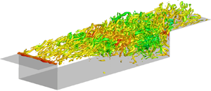



1. Introduction
Flows over open cavities are full of rich physics owing to the natural feedback mechanism imposed on top of broadband turbulence. Disturbances arise from the cavity leading edge and form large vortical structures in the shear-layer region due to the amplification of Kelvin–Helmholtz instabilities. These large-scale structures impinge on the cavity trailing edge, generating strong acoustic waves and intense pressure fluctuations. The acoustic waves propagate upstream over the cavity in subsonic regions, instigate the Kelvin–Helmholtz instabilities in the shear layer, and produce a self-sustained feedback oscillation. In the case of supersonic cavity flow, the fluctuations are accentuated by the appearance of shock waves, which can cause structural damage (Mcgregor & White Reference Mcgregor and White1970). Because cavity flows appear in a wide range of engineering applications, including landing gear wells, aircraft bays, vehicle sun roofs and high-speed trains, there is a strong interest in attenuating the pressure fluctuations over the cavity with flow control techniques (Rowley & Williams Reference Rowley and Williams2006; Cattafesta et al. Reference Cattafesta, Song, Williams, Rowley and Alvi2008).
A large number of studies have focused on analysing the shear layer over the cavity in an attempt to explain the cavity flow unsteadiness. Krishnamurty (Reference Krishnamurty1955) described the resonant oscillations associated with acoustic tones in cavity flows. Shortly thereafter, Rossiter (Reference Rossiter1964) derived the well known semiempirical formula to predict the frequencies of the anharmonic resonant tones in cavity flows, which was slightly modified by Heller, Holmes & Covert (Reference Heller, Holmes and Covert1971). Extensive research has since been carried out to understand the amplitude and other characteristics of cavity flows for different cavity geometries, incoming flow conditions and Reynolds numbers (Rockwell & Naudascher Reference Rockwell and Naudascher1979; Colonius Reference Colonius2001; Rowley & Williams Reference Rowley and Williams2006; Lawson & Barakos Reference Lawson and Barakos2011).
As visible flow structures emerge in cavity flows, modal analysis techniques have been applied to extract the dominant flow features and to understand the underlying flow mechanisms (Taira et al. Reference Taira, Brunton, Dawson, Rowley, Colonius, McKeon, Schmidt, Gordeyev, Theofilis and Ukeiley2017, Reference Taira, Hemati, Brunton, Sun, Duraisamy, Bagheri, Dawson and Yeh2020a; Taira, Hemati & Ukeiley Reference Taira, Hemati and Ukeiley2020b). Subsonic cavity flow fields obtained from experiments have been examined by Murray, Sällström & Ukeiley (Reference Murray, Sällström and Ukeiley2009) with a purely spatial application of the proper orthogonal decomposition (POD). Their analysis revealed that the most energetic modes are the shear-layer modes, whose spatial structures remain similar throughout the subsonic regime. In addition to the primarily two-dimensional shear-layer mode associated with the Kelvin–Helmholtz instability, a three-dimensional centrifugal instability stemming from the large recirculation inside the cavity has been analysed with experimental (Plumblee, Gibson & Lassiter Reference Plumblee, Gibson and Lassiter1962; Maull & East Reference Maull and East1963; Faure et al. Reference Faure, Adrianos, Lusseyran and Pastur2007, Reference Faure, Pastur, Lusseyran, Fraigneau and Bisch2009; Larchevêque, Sagaut & Labbé Reference Larchevêque, Sagaut and Labbé2007) and numerical approaches (Brès & Colonius Reference Brès and Colonius2008; De Vicente et al. Reference De Vicente, Basley, Meseguer-Garrido, Soria and Theofilis2014; Sun et al. Reference Sun, Taira, Cattafesta and Ukeiley2017a). Faure et al. (Reference Faure, Adrianos, Lusseyran and Pastur2007) revealed the evidence of three-dimensional structures inside of the cavity. They showed that the dynamics of the structures were not due to the secondary shear layer instabilities. Brès & Colonius (Reference Brès and Colonius2008) used biglobal instability analysis (Theofilis Reference Theofilis2011) to examine three-dimensional (spanwise) instability of the two-dimensional mean cavity flow. The identified spanwise (centrifugal) instability within the cavity possesses a frequency that is an order of magnitude lower than those associated with the two-dimensional shear-layer instabilities. Recent studies have examined the influence of Mach number and sidewalls on the low-frequency oscillation inside the cavity (Beresh, Wagner & Casper Reference Beresh, Wagner and Casper2016; Liu, Gómez & Theofilis Reference Liu, Gómez and Theofilis2016; Sun et al. Reference Sun, Taira, Cattafesta and Ukeiley2017a,Reference Sun, Taira, Cattafesta and Ukeileyb; Picella et al. Reference Picella, Loiseau, Lusseyran, Robinet, Cherubini and Pastur2018).
Numerous passive and active control strategies have been developed with varying degrees of success to suppress the dominant oscillations (Cattafesta et al. Reference Cattafesta, Song, Williams, Rowley and Alvi2008). A few examples are highlighted below to demonstrate the persistent need for physics-based studies to guide flow control actuation design. Ukeiley et al. (Reference Ukeiley, Ponton, Seiner and Jansen2004) performed an experiment with a small cylinder suspended above the leading edge of the cavity following the work of McGrath & Shaw (Reference McGrath and Shaw1996). The results showed that lifting the shear layer away from the cavity led to significant suppression of the pressure fluctuations, but the performance was highly dependent on the placement of the cylinder. Sarno & Franke (Reference Sarno and Franke1994) used a static fence along the leading edge of the cavity to manipulate the shear layer and suppress the cavity flow oscillations. However, the magnitude of suppression was again highly dependent on the modal frequency and the flow conditions. This phenomenon of suppression degradation associated with a deviation from the design condition is a common characteristic of passive flow control strategies.
Active flow control can provide adaptive capability over a wide range of flow conditions (Colonius Reference Colonius2001; Rowley & Williams Reference Rowley and Williams2006; Cattafesta & Sheplak Reference Cattafesta and Sheplak2011). Vakili & Gauthier (Reference Vakili and Gauthier1994) experimentally studied the effectiveness of steady injection from the leading edge to control the unsteadiness in supersonic cavity flow. Moreover, recent studies have investigated the effect of spanwise spatial variations of steady blowing, which showed that the three-dimensional steady injection outperforms its two-dimensional counterpart in terms of suppression and efficiency (Lusk, Cattafesta & Ukeiley Reference Lusk, Cattafesta and Ukeiley2012; George et al. Reference George, Ukeiley, Cattafesta and Taira2015; Sun et al. Reference Sun, Liu, Cattafesta, Ukeiley and Taira2019; Zhang et al. Reference Zhang, Sun, Arora, Cattafesta, Taira and Ukeiley2019). Rizzetta & Visbal (Reference Rizzetta and Visbal2003), for example, performed a number of large-eddy simulations (LES) on the suppression of cavity flow oscillations using pulsed injection at very high frequency. This type of control suppresses resonant acoustic oscillations with even lower energy input compared with steady injection, but high-frequency forcing at sufficient amplitude in high-speed flows remains a challenge for current actuators (Cattafesta & Sheplak Reference Cattafesta and Sheplak2011). While there have been a number of similar studies on unsteady control of cavity flows, there has not been a systematic investigation on the input–output characterization of high-speed cavity flows with a focus on both forcing frequency and three-dimensionality.
To shed light on these open questions, the present study considers the use of resolvent analysis (Trefethen et al. Reference Trefethen, Trefethen, Reddy and Driscoll1993; Jovanović & Bamieh Reference Jovanović and Bamieh2005) with respect to the time-averaged base flow (McKeon & Sharma Reference McKeon and Sharma2010). Nakashima, Fukagata & Luhar (Reference Nakashima, Fukagata and Luhar2017) capitalized on resolvent analysis to elucidate the control mechanism of the suboptimal control on coherent structures in the wall-bounded turbulent flows. Yeh & Taira (Reference Yeh and Taira2019) used the insights from resolvent analysis to design active thermal actuation to suppress flow separation over an airfoil. They used the response mode and the gain from resolvent analysis to form a metric to quantify momentum mixing and to select control parameters. The chosen control parameters were shown to identify effective control set-ups with companion LES.
Resolvent analysis has also been used by Leclercq et al. (Reference Leclercq, Demourant, Poussot-Vassal and Sipp2019) to design a closed-loop strategy to suppress oscillations in a two-dimensional laminar cavity flow. However, additional progress is required to develop resolvent-analysis-based flow control approaches for high-speed turbulent cavity flow, which possesses complex physics beyond the two-dimensional, laminar, incompressible flow. In the present study, we demonstrate the use of resolvent analysis as a physics-driven approach to systematically design an effective open-loop control technique for supersonic turbulent cavity flows with rich three-dimensional turbulence and shock dynamics. A design metric is introduced to evaluate the effectiveness of perturbation amplification over the length of the cavity, which sheds light on the appropriate parameter space for flow control. Thereafter, we perform LES of controlled flows according to the identified control parameters based on the resolvent-based design metric. The achieved control effects in terms of pressure fluctuation reduction over the cavity are evaluated. The design metric in this work is treated as a necessary condition for effective control but not a sufficient condition to identify the optimal set-up, which calls for validation with companion LES, albeit being a reduced number of cases to consider. This is expected as the high-speed cavity flow at the considered Reynolds number is turbulent (nonlinear) with a broad range of spatiotemporal scales. We also analyse the underlying control mechanisms by studying the coherent structures using the dynamic mode decomposition (DMD) (Rowley & Williams Reference Rowley and Williams2006; Schmid Reference Schmid2010).
The current paper is organized as follows. We present in § 2 the details of the open cavity flow problem, the open-loop control set-up and the resolvent analysis framework. Turbulent supersonic cavity flow characteristics, the properties of the response and forcing modes from resolvent analysis, and three-dimensional dynamic coherent structures are presented and examined in § 3 to identify effective control parameters for unsteady cavity open-loop flow control. Based on the insights gained from resolvent analysis, we then perform a series of controlled cavity flow simulations, illustrate the underlying control mechanism, and correlate the control effect to the resolvent mode in § 4. Finally, concluding remarks are offered in § 5.
2. Approaches
2.1. Problem set-up
We consider spanwise-periodic supersonic turbulent flows over a rectangular cavity with a length-to-depth ratio of  $L/D = 6$ at a free stream Mach number of
 $M_\infty \equiv u_\infty /a_\infty =1.4$, where
 $u_\infty$ and
 $a_\infty$ are the free stream velocity and sound speed, respectively. The Reynolds number based on the cavity depth is
 $Re \equiv \rho _\infty u_\infty D/\mu _\infty =10\,000$ with
 $\rho _\infty$ and
 $\mu _\infty$ being the free stream density and dynamic viscosity, respectively. In the present study, all variables are non-dimensionalized; namely, lengths by the cavity depth
 $D$, temperature by
 $T_\infty$, pressure by
 $(\rho _\infty u_\infty ^{2})/2$, density by
 $\rho _\infty$ and time by
 $D/u_\infty$. The initial boundary layer thickness at the leading edge is set to be
 $\delta _0/D=0.167$. The domain has spanwise periodic boundary conditions imposed with a spanwise periodicity of
 $W/D = 2$. The results using the present computational set-up exhibited good agreement with experimental results (Zhang et al. Reference Zhang, Sun, Arora, Cattafesta, Taira and Ukeiley2019) in which the width of cavity is equal to the spanwise extent of test section in the wind tunnel. The sidewall effects have been investigated rigorously in our past study (Sun et al. Reference Sun, Liu, Cattafesta, Ukeiley and Taira2019). The sidewalls influence the amplitudes of the Rossiter resonant tones but not the frequencies. Moreover, the qualitative control effectiveness is not significantly influenced by the spanwise boundary condition (spanwise periodicity or no-slip sidewall). Hence, the use of spanwise periodic boundary conditions in the present work is appropriate to capture the important flow features.
We study the turbulent cavity flow with LES using a compressible flow solver, CharLES (Khalighi et al. Reference Khalighi, Ham, Moin, Lele and Schlinker2011; Brès et al. Reference Brès, Ham, Nichols and Lele2017). The solver is based on a second-order finite-volume discretization and a third-order Runge–Kutta time integration scheme. For the present LES, Vremen's subgrid scale model (Vreman Reference Vreman2004) is utilized and the Harten–Lax–van Leer contact scheme (Toro, Spruce & Speares Reference Toro, Spruce and Speares1994) is used to capture shocks in the supersonic flows. Random Fourier modes are superimposed to the one-seventh power law velocity profile to simulate unsteady fluctuations from the inlet (Bechara et al. Reference Bechara, Bailly, Lafon and Candel1994). No-slip and adiabatic wall boundary condition is specified along the cavity walls. A sponge boundary condition is applied at the far field and outlet boundaries to damp out exiting waves and prevent numerical reflections.
The computational set-up for the present study is shown in figure 1. A Cartesian coordinate system is used with its origin placed at the spanwise centre of the cavity leading edge, with  $x$,
 $y$ and
 $z$ denoting the streamwise, wall-normal and spanwise directions, respectively. The computational domain extends upstream and downstream by three and seven times of the cavity depth, respectively. The far field extent is set to be nine times of the cavity depth. The computational domain is discretized with a structured mesh with
 $14\,000\,000$ cells for the baseline and
 $16\,000\,000$ cells for the controlled simulations, for which mesh refinement is applied in the vicinity of the actuators. This computational set-up has been verified to accurately characterize flow properties observed in experimental studies (Sun et al. Reference Sun, Liu, Cattafesta, Ukeiley and Taira2019; Zhang et al. Reference Zhang, Sun, Arora, Cattafesta, Taira and Ukeiley2019). A small three-dimensional domain, labelled as domain B in figure 1, is used for the modal analyses. It has a upstream length equal to the cavity depth. The downstream and far field boundaries are placed five times of cavity depth away. The grid size for domain B is approximately
 $70\,000$ cells.
Set-up for computational domain and boundary conditions. Domain A is used for the baseline and controlled LES cases. Domain B is used for resolvent and DMD analyses. The right-hand insert depicts the unsteady actuation control profile for  $\beta _c={\rm \pi}$. The figure is not to scale.

2.2. Unsteady actuation set-up
We perform active control of the cavity flow by introducing unsteady blowing and suction along the leading edge of the cavity through a mass flux boundary condition, as illustrated by the blue dashed line in figure 1. The actuator is located at  $x_c =-0.0698/D$ with a streamwise slot extent of
 $\varLambda _c =0.0175/D$ following our previous experimental studies (Lusk et al. Reference Lusk, Cattafesta and Ukeiley2012; George et al. Reference George, Ukeiley, Cattafesta and Taira2015; Zhang et al. Reference Zhang, Sun, Arora, Cattafesta, Taira and Ukeiley2019). The unsteady actuation is prescribed with a wall-normal velocity profile of
 \begin{equation} u_{jet}(x,z,t) = A\sin(\omega_c t) \varPhi(x,x_c,\varLambda_c)\cos(\beta_c z), \end{equation}
where  $A$ is the actuation amplitude,
 $\omega _c$ and
 $\beta _c$ are the actuation frequency and spanwise wavenumber, respectively. In what follows, we report the actuation frequency
 $\omega _c$ through its dimensionless cavity length-based Strouhal number
 $St_c=\omega _c L/(2{\rm \pi} u_\infty )$. The spatial velocity profile for the actuator is given by
 \begin{align} \varPhi(x,x_c,\varLambda_c) = \tfrac{1}{4}\left\{1+\tanh\left[\kappa_1(x-x_c+\varLambda_c/\kappa_2)\right]\right\} \left\{1-\tanh\left[\kappa_1(x-x_c-\varLambda_c/\kappa_2)\right]\right\} \end{align}
along the streamwise direction to avoid the velocity discontinuity at the edge of the actuator. Here, we choose  $\kappa _1 = 2000$ and
 $\kappa _2 = 2.6$. The actuation frequency and spanwise wavenumber will be selected based on the resolvent analysis as discussed later in § 2.3.
The actuation efforts in this study are reported in terms of the unsteady momentum coefficient defined by
 \begin{equation} C_\mu' \equiv \frac{J}{\frac{1}{2} \rho_\infty u^{2}_\infty W\delta_0}, \end{equation}
where  $J = (\rho _\infty \omega _c/2{\rm \pi} ) \int _{T_c} \int _S u_{jet}(x,z,t)^{2}\,\textrm {d}s\,\textrm {d}t$ is the integral of momentum over the actuation area
 $S$ and the period of the unsteady control actuation
 $T_c=2{\rm \pi} /\omega _c$. The denominator is the equivalent incoming free stream momentum through the boundary layer height at the leading edge of the cavity. In the present study, we set the unsteady momentum coefficient to be
 $C_\mu '=0.02$, following canonical values from past unsteady control studies (Shaw Reference Shaw1998; Williams, Cornelius & Rowley Reference Williams, Cornelius and Rowley2007; Elimelech, Vasile & Amitay Reference Elimelech, Vasile and Amitay2011).
The control effects are assessed using the surface integrated root mean square (r.m.s.) pressure on the aft and bottom walls ( $\tilde {\varOmega }$) defined as
 \begin{equation} \Delta \tilde{p}_{rms}=\frac{(\tilde{p}_{rms,c}-\tilde{p}_{rms})}{\tilde{p}_{rms}}, \quad \text{where} \ \tilde{p}_{rms} = \int_{\tilde{\varOmega}} \frac{p_{rms}}{\frac{1}{2}\rho_\infty u^{2}_\infty}\,\text{d}S \end{equation}
and  $\tilde {p}_{rms,c}$ is the surface integrated pressure fluctuation for the controlled cavity flows. The variable
 $\Delta \tilde {p}_{rms}$ quantifies the relative change of normalized r.m.s. pressure fluctuations over the cavity walls. Later in this paper, we show via resolvent analysis that the above actuator location is indeed appropriate for amplifying the injected perturbation over the cavity.
2.3. Resolvent analysis
Resolvent analysis is used to reveal the flow response to harmonic forcing input with respect to a given base state. In the analysis, we assume the flow  $\boldsymbol{q}(\boldsymbol{x},t)$ can be expressed through Reynolds decomposition
 \begin{equation} \boldsymbol{q}(\boldsymbol{x},t)=\boldsymbol{\bar{q}}(\boldsymbol{x})+ \boldsymbol{q}'(\boldsymbol{x},t), \end{equation}
where  $\boldsymbol{\bar{q}}(\boldsymbol {x})$ is the time-invariant base state and
 $\boldsymbol{q}'(\boldsymbol {x},t)$ is the fluctuation. Traditionally, the base state
 $\boldsymbol{\bar{q}}$ is taken to be an equilibrium state (Trefethen et al. Reference Trefethen, Trefethen, Reddy and Driscoll1993; Jovanović & Bamieh Reference Jovanović and Bamieh2005; Trefethen & Embree Reference Trefethen and Embree2005). In the present study, we consider the time-averaged turbulent cavity flow as the base state with fluctuations being statistically stationary (McKeon & Sharma Reference McKeon and Sharma2010).
By substituting the Reynolds decomposed state variable (2.5) into the Navier–Stokes equations, the governing equation for the fluctuation  $q'$ becomes
 \begin{equation} \frac{\partial \boldsymbol{q}'}{\partial t}=\boldsymbol{\mathsf{L}}(\boldsymbol{\bar{q}})\boldsymbol{q}'+\boldsymbol{f}', \end{equation}
where  $\boldsymbol{\mathsf{L}}(\boldsymbol {\bar{q}})$ denotes the compressible linearized Navier–Stokes operator about
 $\boldsymbol{\bar{q}}$. Here,
 $\boldsymbol{f}'$ is viewed as the forcing input comprised of the sum of remaining terms including the nonlinear terms, which can be interpreted as internal forcing in turbulent flow about the base state due to nonlinear interactions (McKeon & Sharma Reference McKeon and Sharma2010).
In the present study, we consider the three-dimensional turbulent cavity flow with spanwise periodic boundary conditions. Hence, the time- and spanwise-averaged flow is used as the base state  $\boldsymbol{\bar{q}}$. The fluctuation
 $\boldsymbol{q}'$ and forcing
 $\boldsymbol{f}'$ are expressed as Fourier modes with real spanwise wavenumber
 $\beta$ and frequency
 $\omega$ such that
 \begin{equation} \boldsymbol{q}'(\boldsymbol{x},t) =\boldsymbol{\hat{q}}(x, y) \exp\left({\text{i}(\beta z + \omega t)}\right), \quad \boldsymbol{f}'(\boldsymbol{x},t) = \boldsymbol{\hat{f}}(x,y)\exp\left({\text{i}(\beta z+\omega t)}\right). \end{equation}
Note that the dimensional spanwise wavenumber  $\beta _c$ is related to the spanwise wavelength of the control disturbance by
 $\beta _c=2{\rm \pi} /\lambda _c$ and is normalized as
 $\beta =\beta _c D$ such that
 $\lambda _c/D=2{\rm \pi} /\beta$.
Substituting the modal expressions (2.7a,b) into (2.6), we can find the relationship between the forcing  $\boldsymbol{\hat{f}}(x,y)$ and the fluctuation
 $\boldsymbol{\hat{q}}(x,y)$ for each combination of
 $(\omega , \beta )$:
 \begin{equation} \boldsymbol{\hat{q}}_{\omega,\beta} = [\text{i}\omega \boldsymbol{\mathsf{I}} - \boldsymbol{\mathsf{L}}(\boldsymbol{\bar{q}}, \beta)]^{{-}1}\,\boldsymbol{\hat{f}}_{\!\!\omega,\beta} = \boldsymbol{\mathsf{H}}(\boldsymbol{\bar{q}}; \omega, \beta)\,\boldsymbol{\hat{f}}_{\!\!\omega,\beta}. \end{equation}
Here, the operator  $\boldsymbol{\mathsf{H}}(\boldsymbol{\bar{q}}; \omega , \beta ) \equiv [\text {i}\omega \boldsymbol{\mathsf{I}} - \boldsymbol{\mathsf{L}}(\boldsymbol{\bar{q}}, \beta )]^{-1}$ is referred to as the resolvent operator, which serves as the transfer function between the forcing (input)
 $\,\boldsymbol{\hat{f}}_{\!\!\omega ,\beta }$ and the response (output)
 $\boldsymbol{\hat{q}}_{\omega ,\beta }$ about the base state
 $\boldsymbol{\bar{q}}$ for the given frequency
 $\omega$ and spanwise wavenumber
 $\beta$ (Jovanović & Bamieh Reference Jovanović and Bamieh2005; McKeon & Sharma Reference McKeon and Sharma2010; Schmid & Henningson Reference Schmid and Henningson2012).
Since the resolvent operator serves as the transfer function between the response (output) and the forcing (input), the stability property of the transfer function, more specifically the linear operator  $\boldsymbol{\mathsf{L}}(\boldsymbol{\bar{q}},\beta )$, must be evaluated first. We perform stability analysis on the linear operator
 $\boldsymbol{\mathsf{L}}(\boldsymbol{\bar{q}},\beta )$ to examine if the flow system is stable or unstable. The analysis forms an eigenvalue problem as
 \begin{equation} \boldsymbol{\mathsf{L}}(\boldsymbol{\bar{q}};\beta)\boldsymbol{\hat{q}}_\beta=\lambda \boldsymbol{\hat{q}}_\beta , \end{equation}
where  $\lambda =\lambda _r+\text {i} \lambda _i$ with
 $\lambda _i$ representing the temporal frequency of the perturbation and
 $\lambda _r$ being the growth (
 $\lambda _r>0$) or decay (
 $\lambda _r<0$) rate of the perturbation.
For a stable base state ( $\lambda _r<0$ for all
 $\lambda$), we can directly perform resolvent analysis to examine asymptotic energy amplification in the flow system to the harmonic forcing. However, for an unstable base state, perturbations grow exponentially for this linear framework and overshadow the system response to the harmonic forcing (although the fluctuations will saturate in the full nonlinear flow). Thus, care is needed to obtain meaningful physical insight from resolvent analysis. Hence, we focus on highlighting amplifications that occur on a shorter time scale than any existing instabilities with respect to the base flow. Here, we consider the use of exponential discounting (Jovanović Reference Jovanović2004; Yeh et al. Reference Yeh, Benton, Taira and Garmann2020) to analyse the unstable base flow. This discounting approach applies a temporal damping
 $\textrm {e}^{-\kappa t}$ to the variables in (2.6) as
 $[\boldsymbol{q}'_\kappa ,\boldsymbol{f}'_{\!\!\kappa} ] = \textrm {e}^{-\kappa t}[\boldsymbol{q}',\boldsymbol{f}']$. Upon substitution, we arrive at an input–output relation between the Fourier-transformed discounted variables
 $\boldsymbol{\hat{q}}_{\kappa ,\omega ,\beta }$ and
 $\,\hat f_{\kappa ,\omega ,\beta }$ as
 \begin{equation} \boldsymbol{\hat{q}}_{\kappa,\omega,\beta} = \mathcal{H}(\boldsymbol{\bar{q}};\kappa, \omega, \beta) \,\boldsymbol{\hat{f}}_{\!\!\kappa,\omega,\beta}, \end{equation}
with the discounted resolvent operator
 \begin{equation} \mathcal{H}(\boldsymbol{\bar{q}};\kappa, \omega, \beta) =[(\kappa + \text{i}\omega) \boldsymbol{\mathsf{I}}- \boldsymbol{\mathsf{L}}(\boldsymbol{\bar{q}}; \beta)]^{{-}1}. \end{equation}
The discounted resolvent analysis is performed by choosing the discounting parameter  $\kappa > \max (\lambda _r)$ to characterize the forcing-response process over a shorter time scale than the dominant base-flow instabilities.
The discounting approach can be viewed as performing the analysis on a modified linear operator where all of its eigenvalues are shifted towards the stable plane by the discounting parameter  $\kappa$ (Yeh & Taira Reference Yeh and Taira2019). Alternatively, an eddy-viscosity model for the nonlinear internal forcing can also be considered (Reynolds & Hussain Reference Reynolds and Hussain1972; Morra et al. Reference Morra, Semeraro, Henningson and Cossu2019; Pickering et al. Reference Pickering, Rigas, Sipp, Schmidt and Colonius2019). Compared with the discounting approach where the damping is a constant over the frequency–wavenumber space, eddy-viscosity models introduce stronger damping for higher wavenumbers and frequencies. In the present context of flow control, we choose the discounting approach to focus on energy amplifications that occur faster than any existing base-flow instabilities, instead of the frequency and wavenumber-dependent damping technique.
To assess the optimal energy amplification of the system, the resolvent analysis is cast in the framework of singular value decomposition (SVD) of the resolvent operator  $\mathcal{H}$ under the compressible energy norm (Chu Reference Chu1965)
 \begin{equation} E=\int_S \left[\frac{\bar{a}^{2} \rho^{2}}{\gamma \bar{\rho}}+\bar{\rho}({u}^{2}+{v}^{2}+{w}^{2}) + \frac{\bar{\rho}C_v T^{2}}{\bar{T}} \right]\,{\text d}s, \end{equation}
which yields
 \begin{equation}
\boldsymbol{\mathsf{W}}_e^{\frac{1}{2}}\mathcal{H}(\boldsymbol{\bar{q}}; \omega, \beta)\boldsymbol{\mathsf{W}}_e^{-\frac{1}{2}} =
\boldsymbol{\mathsf{Q}} \boldsymbol{\Sigma} \boldsymbol{\mathsf{F}}^{\ast},
\end{equation}
where  $\boldsymbol{\mathsf{W}}_e$ is the weight matrix based on the compressible energy weight above and
 $S$ is the area of analysis as illustrated in figure 1. The matrix
 $\boldsymbol{\mathsf{Q}}=[\boldsymbol{\hat{q}}_1, \boldsymbol{\hat{q}}_2,\ldots , \boldsymbol{\hat{q}}_n]$ holds the set of response modes and the right matrix
 $\boldsymbol{\mathsf{F}}=[\,\boldsymbol{\hat{f}}_{\!\!1}, \boldsymbol{\hat{f}}_{\!\!2},\ldots , \boldsymbol{\hat{f}}_{\!\!n}]$ contains the set of forcing modes. The superscript
 $\ast$ denotes the Hermitian transpose. The singular values
 $\boldsymbol{\Sigma} =\text {diag}(\sigma _1,\sigma _2,\ldots ,\sigma _n)$ represent the amplification between the response and forcing modes in descending order. The SVD is performed within the ARPACK package with a Krylov space of 32 vectors and a residual tolerance of
 $10^{-7}$. The results converge to at least seven significant figures and verified to be independent with respect to the domain size and mesh resolution (Sun et al. Reference Sun, Liu, Cattafesta, Ukeiley and Taira2020).
3. Uncontrolled cavity flow
3.1. Baseline flow characteristics
The baseline supersonic turbulent flow over the rectangular cavity at  $M_\infty =1.4$ and
 $Re=10\,000$ is considered. The instantaneous flow is visualized in figure 2 using an isosurface of the
 $Q$-criterion coloured by the pressure coefficient. The background shows the numerical schlieren with
 $\| \boldsymbol {\nabla } \rho \|$ to capture the waves. The incoming flow forms a shear layer that emanates from the leading edge of the cavity. The shear layer rolls up into large spanwise vortices at approximately one third of the cavity length, generating large fluctuations over the cavity. Once the large spanwise vortices reach the middle of the cavity, there is a loss of spanwise coherence corresponding to the emergence of small-scale vortical structures. In supersonic cavity flows, the large-scale structures obstruct the free stream and create compression waves. Moreover, the impingement of these vortical structures onto the aft cavity wall generates strong waves that travel upstream within the subsonic region. The vortical and pressure fluctuations produce a high level of unsteadiness in and above the cavity. Towards the aft of the cavity, there is a complex interplay between the shear layer, the impingement of the vortical structures on the aft wall, and the recirculation within the cavity.
Instantaneous cavity flow visualized with the  $Q$-criterion
 $Q(D/u_\infty )^{2}=10$ coloured by
 $C_p=(p-p_\infty )/((\rho _\infty u^{2}_\infty )/2)$ at
 $M_\infty =1.4$. Numerical schlieren is shown in the background in greyscale.

High levels of unsteadiness emerge along the aft wall due to the impingement of vortical structures and within the shear layer from the formation of the large-scale vortical structures. The normalized r.m.s. pressure fluctuations are presented in figure 3(a). Here, the large r.m.s. levels along the cavity trailing edge are seen in the shear layer near the middle ( $2\lesssim x/D \lesssim 4$) of the cavity and above the cavity from the unsteady compression waves.
(a) The r.m.s. pressure,  $p_{rms}/((\rho _\infty u^{2}_\infty )/2)$, along the cavity surfaces and
 $x$–
 $y$ plane along
 $z/D=-1$. (b) Power spectral analysis of pressure
 $p/((\rho _\infty u^{2}_\infty )/2)$ at three probe locations along the shear layer. The shading indicates uncertainty bounds representing
 $95\,\%$ confidence intervals. The predicted Rossiter mode frequencies from (3.1) are indicated by the black dashed lines.

Power spectral densities of the fluctuations at three representative locations of  $(x, y, z)/D =(0.75, 0, 0)$,
 $(3, 0, 0)$ and
 $(5.25, 0, 0)$ along the shear layer are shown in figure 3(b). Welch's method is used with a frequency resolution of 16 Hz, a Hanning window and 75 % overlap. The dominant oscillation frequency shifts as the flow advects over the cavity. We can compare the spectra with the resonance frequencies predicted by the modified Rossiter's semiempirical formula (Heller et al. Reference Heller, Holmes and Covert1971)
 \begin{equation} St_L=\frac{fL}{u_\infty} =\frac{n-\alpha}{1/k + M_\infty /\sqrt{1+(\gamma-1)M_\infty^{2}/2}}, \end{equation}
where the specific heat ratio is  $\gamma =1.4$, the average convection speed of disturbances in shear layer is
 $k=0.65$ and the phase delay
 $\alpha =0.38$ (Zhang et al. Reference Zhang, Sun, Arora, Cattafesta, Taira and Ukeiley2019) for the
 $n$th Rossiter mode. At
 $x/D=0.75$, the primary oscillation appears at
 $St_L=0.6$ with a low amplitude. Once the flow reaches
 $x/D=3$, the dominant frequency corresponds to Rossiter mode IV, whose Strouhal number is
 $St_L=1.33$. At the trailing edge, the dominant frequency shifts to the lower Rossiter mode II frequency
 $St_L=0.6$, with a substantial reduction in the oscillation amplitude. The shift in the dominant oscillation frequency as the vortical structures convect over the cavity suggests strong nonlinear interactions in the flow.
To identify the flow structures corresponding to the peak frequencies, we perform DMD (Rowley et al. Reference Rowley, Mezić, Bagheri, Schlatter and Henningson2009; Schmid Reference Schmid2010) on the snapshots of the flow field. The DMD analysis is performed on the whole three-dimensional flow field, without decomposing the flow into spanwise Fourier components. The whole flow field is examined with DMD to study the possibility of spanwise mixing for each frequency, which becomes important when we later assess flow control effects. Convergence of the DMD modes was ensured by varying the number of snapshots used in the analysis. Both the frequencies and modal structures computed by using the full set of snapshots and half of such data did not exhibit any significant differences, substantiating the discussions to follow.
Isosurfaces of the streamwise velocity component of the DMD modes at the frequencies of  $St_L=0.6$ and
 $1.33$ are shown in figure 4. The DMD modes capture the shear-layer modes associated with the respective single frequency. By comparing the spatial structures for these two frequencies, it is observed that the DMD mode for
 $St_L=0.6$ possesses larger structures in both the streamwise and vertical directions. In contrast, the structures in the DMD mode for
 $St_L = 1.33$ are reduced in size by approximately one half. Noteworthy here is that these two DMD (shear layer) modes exhibit spatial variations with the same dimensionless spanwise wavenumber of
 $\beta ={\rm \pi}$ as seen in the top views of figure 4. In what follows, we perform resolvent analysis on the time-averaged flow and examine the energy amplification of the system to external forcing. We then use the information from DMD and resolvent analysis to guide the design of an effective flow control approach.
Spatial structures of DMD modes visualized with real streamwise velocity isosurface  $(\pm 0.3)$ with (a,c)
 $St_L = 0.6$ and (b,d)
 $St_L = 1.33$.

3.2. Resolvent spectra and modes
As we initiate the resolvent analysis of the turbulent cavity flow, stability analysis is first performed on  $\boldsymbol{\mathsf{L}}(\boldsymbol{\bar{q}}; \beta) $ to evaluate its stability properties. The eigenspectra and pseudospectra are shown in figure 5(a,b) for two representative cases with
 $\beta ={\rm \pi}$ and
 $3{\rm \pi}$. The imaginary part of the eigenvalue
 $\lambda$ is normalized as
 $\lambda _i L/(2{\rm \pi} u_\infty )$ and the real part is normalized as
 $\lambda _r D/u_\infty$. The results indicate the linear operator
 $\boldsymbol{\mathsf{L}}(\boldsymbol{\bar{q}}; \beta)$ is unstable with positive growth rates (
 $\lambda _r D/u_\infty > 0$) of the eigenmodes, including both centrifugal and shear-layer modes. The spatial structures of two representative unstable modes, a centrifugal and a shear-layer mode, are shown in figure 5(c). The centrifugal mode is present inside of the cavity, which corresponds to the recirculation (Brès & Colonius Reference Brès and Colonius2008). However, the shear-layer mode appears over the cavity and is formed due to the Kelvin–Helmholtz instability.
(a,b) Eigenspectra and pseudospectra of  $L(\bar {q};\beta )$ for spanwise wavenumbers
 $\beta ={\rm \pi}$ (a) and
 $3{\rm \pi}$ (b). The magenta dots indicate the growth rates and frequencies of
 $L(\bar {q};\beta )$. The dashed line indicates the neutral stability line. The contour plots visualize the pseudospectra. (c) The (1) centrifugal and (2) shear-layer modes visualized by the real component of the streamwise velocity. The locations of their eigenvalues are indicated on panel (a).

We show the pseudospectra contours (Trefethen & Embree Reference Trefethen and Embree2005) of the linear operator  $\boldsymbol{\mathsf{L}}(\boldsymbol{\bar{q}}; \beta)$ as the background in figure 5(a,b). Higher values of contours appear on the left-hand side planes for both cases of
 $\beta ={\rm \pi}$ and
 $3{\rm \pi}$, where the stable eigenvalues are located. For the case of
 $\beta ={\rm \pi}$, pseudospectral levels protrude far into the unstable plane at
 $1<\lambda _i L/(2{\rm \pi} u_\infty ) < 4$ representing non-normal behaviour of the operator. For the case of
 $\beta =3{\rm \pi}$, the non-normal behaviour of the operator occurs in the frequency range of
 $2<\lambda _i L/(2{\rm \pi} u_\infty ) < 5$. The non-normal behaviour of the operator can cause the flow to exhibit significant energy amplification.
Because the linear operator  $\boldsymbol{\mathsf{L}}(\boldsymbol{\bar{q}}; \beta)$ is unstable, we perform a discounted resolvent analysis. The discounting parameter is associated with temporal windowing of the system response to examine the dynamics before the instability diverges, as discussed in § 2.3. The leading and secondary gains for the case of
 $\beta =2{\rm \pi}$ using different discounting parameters of
 $\kappa D/u_\infty =0.1$,
 $0.2$ and
 $0.3$ are shown in figure 6. We observe that, as
 $\kappa D/u_\infty$ increases, the magnitude of resolvent gain decreases. However, the profile of the gain distribution is not altered by the choice of discounting parameter. In fact, the maximum gain is achieved at the same Strouhal number of
 $St_L\approx 3$.
Resolvent gain calculated using discounting parameter of  $\kappa D/u_\infty = 0.1$,
 $0.2$ and
 $0.3$ for
 $\beta =2{\rm \pi}$.

The large separation between the primary and secondary gains ( $\sigma _1$ and
 $\sigma _2$) for
 $St_L > 0.5$ enables the application of the rank-1 assumption in the present study. By using the rank-1 assumption, we focus on the leading gain and its corresponding forcing and response modes (McKeon & Sharma Reference McKeon and Sharma2010; Gómez et al. Reference Gómez, Blackburn, Rudman, McKeon, Luhar, Moarref and Sharma2014; Schmidt et al. Reference Schmidt, Towne, Colonius, Cavalieri, Jordan and Brès2017a). Here we choose the discounting parameter of
 $\kappa D/u_\infty =0.2$ in the resolvent analysis to analyse the unstable system.
The leading singular value versus various combinations of spanwise wavenumber and frequency is presented in figure 7, revealing the optimal energy amplification of harmonic forcing. Larger amplification that emerges around  $2< St_L<4$ and
 ${\rm \pi} /2<\beta <5{\rm \pi} /2$ is apparent in this figure. As Rossiter modes primarily stem from two-dimensional shear-layer instabilities, the gain distribution with
 $\beta =0$ exhibits discrete peaks at the Rossiter mode frequencies, which are consistent with the power spectral density of pressure shown in figure 3 from the nonlinear flow simulation. On the other hand, for spanwise wavenumbers
 $\beta > {\rm \pi}$, the gain exhibits a smoother distribution versus Strouhal number.
The leading energy amplification  $\sigma _1$ over
 $\beta$ and
 $St_L$ for a discount parameter of
 $\kappa D/u_\infty =0.2$.

The representative forcing and response modes are presented in figure 8 for  $\beta ={\rm \pi}$,
 $2{\rm \pi}$ and
 $3{\rm \pi}$ at
 $St_L=0.6$, 2.49 and 5.14 which show the lower, middle and high-frequency cases. The forcing and response modes are shown with the real streamwise component in figure 8(a,b), respectively. The influence of frequency and spanwise wavenumber on mode structures are similar for both forcing and response modes. As the frequency increases, the streamwise structures exhibit a finer pattern. The structures become more compact in the transverse direction as the spanwise wavenumber increases. For the forcing modes, the dominant structures emerge at the leading edge of the cavity. This indicates that the optimal spatial location for the unsteady forcing input is indeed at the leading edge of the cavity, substantiating the actuator location discussed in § 2.2. For the response modes, the structures appear over shear layer region and inside the cavity for the low-frequency case. As the frequency increases, the response mode structures are confined to the shear-layer region.
Real streamwise velocity component of the (a) forcing and (b) response modes at  $St_L=0.6$,
 $2.49$ and
 $5.14$ with
 $\beta ={\rm \pi}$,
 $2{\rm \pi}$ and
 $3{\rm \pi}$.

Wave structures emerge at the leading and trailing edges of the cavity for the case of  $(\beta , St_L)=({\rm \pi} , 0.6)$. Such wave structures become weaker and disappear for larger values of
 $\beta$. This change is due to the two-dimensional property of compression waves. As the spanwise wavenumber increases, the three-dimensionality suppresses the generation of two-dimensional compression waves. For the case of
 $St_L=2.49$, the compression waves structures disappear. For higher frequencies, the compression waves appear at the leading edge, as shown for the cases of
 $({\rm \pi} , 5.14)$ and
 $(2{\rm \pi} , 5.14)$. The higher frequency forcing magnifies the obstruction effect at the leading edge, which results in the formation of compression waves in the response structures.
4. Controlled cavity flows
In this section, the findings from the above resolvent and DMD analyses are used to design open-loop active flow control strategies for the attenuation of intense pressure fluctuations. The performance of the flow control techniques is then assessed through nonlinear LES. For all controlled cases considered below, the oscillatory momentum coefficient defined in (2.1) is fixed at  $0.02$. While the primary effort here is to reduce pressure fluctuations at
 $Re=10\,000$, we desire a control approach that can generalize to higher Reynolds numbers, thereby favouring case with the largest reduction. Therefore, we seek effective control set-ups, especially those that perform exceptionally well and that can be promising for more challenging flow set-ups in future studies.
4.1. Resolvent-analysis-based active flow control design
As discussed above, the DMD analysis reveals the coherent structures that are responsible for large-scale unsteadiness over the cavity. In a complementary manner, the resolvent analysis identifies structures that can be amplified through sustained forcing. Here, we look for the means to identify candidate input perturbations that will amplify over the cavity and inhibit the generation of the natural large-scale spanwise vortical structures identified by DMD. It should be noted that resolvent analysis is a linear analysis technique which essentially acts as a model for the nonlinear turbulent cavity flow with active flow control input. We therefore anticipate some differences but do not consider them to lead to substantial contradictions that prevent achievement of the objective of determining an effective control set-up. We emphasize that resolvent-analysis-based guidelines discussed herein should be treated as a necessary condition, but not as a sufficient condition to achieve effective flow modification. This means that the control parameter search space can be significantly reduced but requires careful assessment with companion LES (or experiments).
The DMD analysis of the uncontrolled flow shows that the primary oscillation at a frequency of  $St_L=1.33$ is associated with the dominant spanwise wavenumber of
 $\beta ={\rm \pi}$, as shown in figure 4. The control goal is therefore to force the cavity flow in a sustained manner to disrupt the formation of this undesirable structure. The optimal input disturbance should ideally persist over the entire cavity length without spilling its energy to the naturally energetic structures. It is noteworthy that our previous experiments (Lusk et al. Reference Lusk, Cattafesta and Ukeiley2012) indicated that effective three-dimensional steady blowing persisted over the entire cavity length, while less effective disturbances decayed. A subsequent experimental companion study (Zhang et al. Reference Zhang, Sun, Arora, Cattafesta, Taira and Ukeiley2019) showed that steady blowing actuation introduced counter-rotating vortex pairs in-between blowing slots that distorted the shear layer and inhibited the growth of the large-scale vortical structures, mitigating the impingement effect. However, the control modification decayed towards the rear part of the cavity, which likely limited the control effectiveness. The goal in the present study is hence to select unsteady three-dimensional forcing inputs that persist over the cavity length and do not energize the natural
 $\beta ={\rm \pi}$ disturbances.
Motivated by these previous studies and the results presented thus far, we introduce a guiding metric to assess the integrated kinetic energy along the streamwise direction using the leading response mode,
 \begin{equation} {\hat E}_1(x)=\int_{{-}D}^{\infty} \tfrac{1}{2}\sigma_1^{2} \bar{\rho} \left[ \hat{u}_1\hat{u}_1^{{\ast}}+\hat{v}_1\hat{v}_1^{{\ast}} \right]\,{\text d}y, \end{equation}
where  $\sigma _1$ is the leading gain,
 $\bar {\rho }$ is the time-averaged density, and
 $\hat {u}_1$ and
 $\hat {v}_1$ are the streamwise and vertical components of the response mode, respectively. Their complex conjugate counterparts are denoted as
 $\hat {u}_1^{\ast }$ and
 $\hat {v}_1^{\ast }$. The metric
 $\hat {E}_1$ quantifies the response kinetic energy and assesses the effectiveness of perturbation amplification over the cavity. For an effective amplification mechanism, we should observe a sustained profile of
 $\hat {E}_1$ over the entirety of the cavity shear layer to ensure that the forcing input remains influential over the whole extend of the cavity. We emphasize here that both the high value of
 $\hat {E}_1$ and the sustained profile over the cavity are sought to mitigate the large-scale fluctuations in cavity flow, as we discuss in detail below. This metric should be considered in conjunction with the physical insights gained from baseline LES and DMD analysis, and be viewed as a necessary condition to expect effective modification of the mean flow. This is due to the fact that the resolvent analysis is based on a linearization about the mean flow and can show some differences from the nonlinear cavity flow during the flow control process, for which we should place some care. Saturation of control performance in terms of reduction in pressure fluctuations could exist despite the favourable feature of the metric
 $\hat {E}_1$ due to nonlinear effects in the cavity flow.
The primary kinetic energy amplification profiles  $\hat {E}_1(x)$ over the cavity for representative cases at frequencies of
 $St_L=0.6$,
 $1.2$,
 $2.49$ and
 $5.14$ and spanwise wavenumbers of
 $\beta ={\rm \pi}$,
 $2{\rm \pi}$,
 $3{\rm \pi}$ and
 $4{\rm \pi}$ are shown in figure 9. For the cases at
 $St_L=0.6$, the energy amplification over the cavity maintains a low magnitude, reaching only up to
 $\hat {E}_1 =1000$ compared with cases with other frequencies. As the front part of the cavity (
 $0\le x/D \le 3$) is a critical region for shear-layer roll-ups to develop, the relatively low value of
 $\hat {E}_1$ suggests that control with
 $St_L=0.6$ may not hold sufficient control authority to change the baseline flow feature. Moreover, the distribution gradually increases from the leading edge to the trailing edge and is almost identical for the different spanwise wavenumbers, which indicates that the spanwise wavenumber has limited impact on the magnitude of the primary energy amplification for
 $St_L=0.6$. For the case of
 $St_L=1.2$, the overall magnitudes of
 $\hat {E}_1$ over the cavity are higher than those at
 $St_L=0.6$. The primary energy amplification decreases as the spanwise wavenumber increases and reach its maximum value around
 $x/D \approx 4$.
Kinetic energy amplification profiles based on the primary response mode over the cavity at frequencies of (a)  $St_L=0.6$, (b)
 $1.2$ (c)
 $2.49$ and (d)
 $5.14$ for spanwise wavenumbers of
 $\beta ={\rm \pi} , 2{\rm \pi} , 3{\rm \pi}$ and
 $4{\rm \pi}$.

Next, we turn our attention to the primary energy amplification at a higher frequency of  $St_L = 2.49$. Compared with the previous cases at
 $St_L=0.6$ and 1.2, the energy amplification exhibits a sustained profile and much higher magnitude over the cavity. The perturbations with spanwise wavenumbers of
 $\beta = {\rm \pi}$ and
 $2{\rm \pi}$ are especially prominent. For these cases, the primary kinetic energy amplification remains high over the entire cavity length, with its maximum value attained around the middle of the cavity. Although the magnitudes of
 $\hat {E}_1$ decrease as the spanwise wavenumbers increase, they remain high (
 $\sim O(10^{5}$)) compared with the other frequencies, except for the case of
 $\beta =4{\rm \pi}$ with
 $\hat E_1\approx 2500$. However, given the prominence of the
 $\beta ={\rm \pi}$ structure in the DMD analysis of the baseline, we suspect that introducing a
 $\beta _c=2{\rm \pi}$ disturbance forcing may be the more effective of the two.
For the high-frequency cases of  $St_L=5.14$, the response energy significantly amplifies in the front of the cavity, but decreases past
 $x/D\approx 1$, becoming significantly lower in magnitude towards the rear part of the cavity. This distribution of the response kinetic energy, losing its authority in the rear part of the cavity, is suspected to be indicative of a suboptimal control case. Other coherent structures may emerge when the response kinetic energy is weak to sustainable forcing. For this reason, it appears that such high-frequency forcing will be less effective for the suppression of fluctuations in open cavity flows.
4.2. Assessments of resolvent-analysis-based cavity flow control
Unsteady actuation is introduced in LES for the forcing frequency  $St_c$ and spanwise wavenumber
 $\beta _c$ identified by the resolvent analysis to be potentially effective for flow modification. Because practical forcing cannot be introduced globally, local forcing is imposed along the cavity leading edge, which is where the forcing modes are concentrated, as shown in figure 8(a). In the above discussion, it was revealed that a forcing frequency of
 $St_L=2.49$ with spanwise wavenumbers between
 ${\rm \pi}$ to
 $3{\rm \pi}$ exhibits a sustained and high-valued response kinetic energy
 $\hat {E}_1$ over the cavity based on the resolvent analysis. Large-eddy simulations are performed for this choice of parameters and some other representative cases to assess the effectiveness of the actuation set-up. The resolvent analysis here aids the study by reducing the control parameter search space. We, in particular, consider a forcing frequency and spanwise wavenumber in the range of
 $0.6\le St_c \le 5.14$ and
 ${\rm \pi} \le \beta _c \le 4{\rm \pi}$ for the following validation LES cases. Let us note that the uses of unsteady actuation are likely be effective for many of these cases as long as they disrupt the formation of the large-scale spanwise vortices in the uncontrolled flow. The key question here is to find the near-optimal control case, in which the forcing effect remains influential over the long cavity.
The pressure fluctuations obtained from LES of controlled flows are examined over the cavity surfaces and the shear layer. Intense pressure oscillations appear over these regions in the uncontrolled cavity flow. A number of representative controlled cases are investigated, including the controlled cases with the parameters that are identified to provide sustained forcing over the cavity by resolvent analysis. The pressure fluctuations for the controlled cases are shown in figure 10. Compared with the pressure distribution for the uncontrolled flow, we observe that some of the controlled cases show significant attenuation of the fluctuations over the shear layer and on the cavity walls.
The r.m.s. pressure  $p_{rms}/((\rho _\infty u^{2}_\infty )/2)$ over the cavity surfaces and the
 $x$–
 $y$ plane at
 $z/D=-1$ for the uncontrolled (a) and controlled (b–j) cases.

For the control cases with  $St_c=0.6$, the pressure fluctuations are reduced over the shear-layer region and along the cavity walls compared with the uncontrolled cavity flow. Along the cavity floor, the area experiencing large pressure fluctuations are limited to the aft third of the cavity, which is reduced in size from the uncontrolled case. Above the shear layer, actuation is able to modify the flow field to reduce the spatial extent over which large fluctuations appear, but the unsteady shock-induced fluctuations remain strong over the rear half of the cavity in the case of forcing spanwise wavenumbers of
 $\beta _c = {\rm \pi}$ and
 $2{\rm \pi}$. As the values of metric
 $\hat E_1$ calculated from resolvent analysis for frequency
 $St_c=0.6$ are relatively low (figure 9), the discrepancy in pressure reductions among those cases from
 $\beta ={\rm \pi}$ to
 $3{\rm \pi}$ results from nonlinearity of the flow. Although the case with
 $(\beta _c,St_c)=(3{\rm \pi} ,0.6)$ has a desirable control performance, this scenario may require additional guidance beyond resolvent analysis.
Next, the controlled flows with a forcing frequency of  $St_c=2.49$ are considered. All of the forcing spanwise wavenumbers of
 $\beta _c = {\rm \pi}$,
 $2{\rm \pi}$ and
 $3{\rm \pi}$ shown in figure 10 significantly reduce the pressure fluctuations over the cavity walls as well as the shear layer. Most noteworthy here are the cases where the spanwise wavenumbers of the forcing input are
 $2{\rm \pi}$ and
 $3{\rm \pi}$. For these cases, the unsteady forcing is able to shorten the spatial (vertical) extent of large fluctuations. Due to the stabilizing effect in the shear layer and weakened impingement of flow structures, we observe remarkable reductions in the pressure fluctuations above
 $50\,\%$ along the aft and bottom walls of the cavity (see summary in table 1). Compared with the baseline and the other controlled cases, high levels of pressure fluctuations are experienced only along the trailing edge of the cavity.
Summary of flow control cases with unsteady actuation.

Although at  $St_c=2.49$ the metric
 $\hat E_1$ for
 $\beta =2{\rm \pi}$ is much higher than
 $\beta =3{\rm \pi}$, as shown in figure 9, similar control effectiveness in terms of the level of
 $P_{rms}$ reductions suggest that the control effects are experiencing saturation due to nonlinearities at the frequency of
 $St_c=2.49$. For the case of
 $\beta = 4{\rm \pi}$, the reduction level may appear lower in value, but the
 $E_1$ value is higher than the those for the case of
 $St = 0.6$. The substantial reduction of pressure fluctuations over the cavity is achieved with the choice of control parameters identified from the resolvent (response mode)-based kinetic energy based metric (4.1). This implies that the input–output relationship captured by resolvent analysis for the turbulent cavity flow can indeed point to an effective set of control parameters with significantly less computational resources than what is required by an uninformed parametric LES study.
Forcing at a frequency of  $St_c=5.14$ is also examined, which is higher than the frequency identified by the resolvent analysis. For these controlled cases, the pressure fluctuations over the shear layer are higher in magnitude compared with the cases of
 $St_c=2.49$, as shown in figure 10. These results are expected as the forcing to enhance mixing across the shear layer is not as sustained as in the case of
 $St_c=2.49$, which is indicated by figure 9. In fact, the unsteady control induces the appearance of oblique shocks for all spanwise wavenumber cases shown in figure 10, which renders the control counterproductive. We also observe strong impingement of vortical structures for the spanwise wavenumber of
 $3{\rm \pi}$, which increases the pressure fluctuations on the entire aft wall above that of the uncontrolled case. Note that it is not only the maximum value of
 $E_1$ but also sustained distribution (flatness) of the
 $E_1$ profile are important.
Looking closer at the flow fields for some of the cases presented in figure 10, we visualize in figure 11 the instantaneous vortical structures for effective controlled cases with  $(\beta _c, St_c)=(2{\rm \pi} ,2.49)$ and
 $(3{\rm \pi} ,2.49)$ as well as an ineffective controlled case with
 $(3{\rm \pi} , 5.14)$. Shown in this figure are the isosurfaces of the
 $Q$-criterion coloured by the pressure coefficient. For the case of
 $(\beta _c, St_c)=(2{\rm \pi} ,2.49)$ shown in figure 11(a), small streamwise vortices are generated from the leading edge and propagate downstream, which gradually spread over the shear layer. Large-scale spanwise shear layer roll-ups disappear in the flow field compared with the uncontrolled cavity flow (recall figure 2). The modification of the flow field produced by the unsteady actuation greatly attenuates the large-scale flow structure impingement on the aft-wall by breaking up large structures and reduces the fluctuations over the cavity. The aft wall only experiences small-scale vortical structures hitting the wall in an incoherent manner. As the kinetic energy profile (4.1) foreshadows, the mixing and breakup of the large-scale spanwise vortices are sustained over the entire cavity length and yield an effective control approach to reduce the pressure fluctuations.
Instantaneous controlled cavity flows with (a)  $(\beta _c, St_c)=(2{\rm \pi} ,2.49)$, (b)
 $(3{\rm \pi} ,2.49)$ and (c)
 $(3{\rm \pi} , 5.14)$, visualized with the
 $Q$-criterion
 $Q(D/u_\infty )^{2}=10$ coloured by
 $C_p=(p-p_\infty )/((\rho _\infty u^{2}_\infty )/2)$ at
 $M_\infty =1.4$. Numerical schlieren is shown in the background in greyscale.

For the controlled case with  $(\beta _c, St_c)=(3{\rm \pi} , 2.49)$ presented in figure 11(b), the flow structure appears similar to those from the case of
 $(\beta _c, St_c)=(2{\rm \pi} ,2.49)$. With the choice of a high wavenumber, the structures are generated by the unsteady actuation from the cavity leading edge in a closely packed manner. These streamwise vortical structures appear to cancel the vortical influence from each other due to their close proximity and cannot suppress the spanwise instability from appearing as effectively as the case with
 $(\beta _c, St_c)=(2{\rm \pi} , 2.49)$. This leads to correspondingly larger fluctuations over the cavity and local thickening of the shear layer, as visualized by the wider range of pressure values in figure 11(b).
For the case of  $(\beta _c, St_c)=(3{\rm \pi} ,5.14)$ shown in figure 11(c), the streamwise vortices generated from unsteady actuation are truncated to become shorter than what are observed for the lower frequency actuation. By the middle of the cavity, the shear layer rolls up into a spanwise vortical coherent structure with a size comparable to the cavity depth that penetrates both into the free stream and the cavity. The local obstructions of the incoming flow by these large-scale vortical structures lead to the appearance of strong compression waves, adding to the increased pressure fluctuations over the shear layer and along the cavity walls. Compared with the other controlled cases, strong acoustic waves emitted from the leading edge of the cavity are observable.
The premultiplied pressure spectra visibly exhibit significant pressure fluctuation reductions for the controlled cases, as shown in figure 12. For the two effective control cases of  $(\beta _c, St_c)=(2{\rm \pi} ,2.49)$ and
 $(3{\rm \pi} ,2.49)$, the actuation inputs successfully suppress the tone at
 $St_L=1.33$ in the baseline case and reduce the turbulent pressure fluctuations. Even with a slight magnitude increase at
 $St_L=0.6$ for the case of
 $(3{\rm \pi} ,2.49)$, the actuation effectively suppresses the overall pressure fluctuations due to the substantial reduction of magnitude over other frequency bands. For the ineffective case of
 $(3{\rm \pi} , 5.14)$, the actuation suppresses the tone at
 $St_L=1.33$. However, the apparent increase of pressure fluctuations over the frequency band of
 $St_L<1$ gives rise to strong oscillations over the cavity. Those strong oscillations with
 $St_L<1$ are associated with the larger vortical coherent structures and results in ineffective control outcome.
Premultiplied pressure spectra at midcavity along the shear layer for the controlled flows shown in black. The baseline spectra are shown by the blue dashed lines. Here (a)  $(\beta _c, St_c) = (2{\rm \pi} , 2.49)$, (b)
 $(3{\rm \pi} , 2.49)$ and (c)
 $(3{\rm \pi} , 5.14)$.

It is observed above that the control input influences the shear-layer thickness and consequently the pressure fluctuation level. For this reason, the vorticity thickness
 \begin{equation} \delta_\omega = \frac{u_\infty}{(\partial \bar{u}/\partial y)_{max}} \end{equation}
is considered to quantify the direct influence of the unsteady actuation on cavity flow. Here,  $\bar {u}$ is the spanwise and time-averaged streamwise velocity. Figure 13 shows the vorticity thickness of the shear layer from controlled cases at spanwise wavenumbers of
 $\beta _c={\rm \pi} , 2{\rm \pi}$ and
 $3{\rm \pi}$. For the controlled cases,
 $\delta _\omega$ is thicker at the leading edge compared with the uncontrolled case. This local thickening of the shear layer at the leading edge reduces its receptivity to the acoustic disturbances and stabilizes the shear layer as it advects downstream. For the cases of
 $\beta _c=2{\rm \pi}$, a significant reduction of vorticity thickness is observed in the rear part of the cavity. Note that the sudden decrease in the vorticity thickness near the trailing edge is due to the effect of impingement on the cavity trailing edge.
Vorticity thickness  $\delta _\omega$ for the uncontrolled and controlled cases.

The magnitude of pressure fluctuations inside the cavity is coupled with the pressure fluctuations occurring above the shear-layer region. We quantify the control effectiveness by integrating the pressure fluctuations over the floor and aft-wall of the cavity using (2.4). The unsteady control cases in general achieve significant reductions of pressure fluctuations compared with the uncontrolled case. Particularly noteworthy is the control case with  $(\beta _c, St_c)=(2{\rm \pi} , 2.49)$ which achieves
 $52\,\%$ reduction in the pressure fluctuations, as summarized in table 1. Additionally, the present unsteady control substantially outperforms our previous control efforts using steady three-dimensional actuation (Sun et al. Reference Sun, Liu, Cattafesta, Ukeiley and Taira2019). The trends summarized in table 1 are consistent with the predictive metric for control design, which validates the conceptual approach of how to use the results of the resolvent analysis to determine an effective unsteady flow control set-up.
4.3. DMD of the controlled flows
Let us further assess the influence of unsteady actuation on the turbulent cavity flow using DMD analysis. Here, the DMD analysis serves as an a posteriori analysis of the nonlinear flow with control to assess the control effectiveness and is not meant to provide any direct comparison with resolvent analysis. We extract the coherent structures produced at the forcing frequency to examine the persistence of forcing input (perturbation) from the leading edge of the cavity. Here, the DMD analysis extracts the key flow response structures around the optimal control case for the forcing frequency of  $St_c=2.49$ with spanwise wavenumbers of
 $\beta _c = {\rm \pi}$,
 $2{\rm \pi}$ and
 $3{\rm \pi}$. Presented in figure 14 are the spatial structures of the spanwise velocity associated with the forcing frequency of
 $St_c=2.49$. We also note in passing that, while not shown, the DMD modes are in good agreement with spectral POD modes (Schmidt et al. Reference Schmidt, Towne, Rigas, Colonius and Brès2017b; Schmidt & Colonius Reference Schmidt and Colonius2020) extracted from the controlled flows. By examining the spatial evolution of the DMD modes over the cavity, we can understand the mechanism by which the forcing input prevents the undesirable large-scale vortex roll-up from appearing over the cavity.
Side and top views of the real spanwise velocity of DMD modes for the control cases. Isosurface values of streamwise velocity are  $0.1$ (red) and
 $-0.1$ (blue). Here (a,b)
 $(\beta _c, St_c) = ({\rm \pi} , 2.49)$, (c,d)
 $(2{\rm \pi} , 2.49)$ and (e,f)
 $(3{\rm \pi} , 2.49)$.

Consider the controlled flow case of  $\beta _c={\rm \pi}$, shown in figure 14(a,b). This forcing wavenumber is the same as the dominant spanwise wavenumber observed in figure 4 for the uncontrolled flow. From the top view in figure 14(a,b), we notice that the flow structures essentially maintain the spanwise wavenumber of
 $\beta ={\rm \pi}$, except for some regions over
 $1 \lesssim x/D \lesssim 3$ due to nonlinear interactions. The fact that
 $\beta ={\rm \pi}$ remains the primary wavenumber indicates that the control is ultimately unable to fully attenuate the undesirable fluctuations.
For the case of controlled flow with  $\beta _c=2 {\rm \pi}$, shown in figure 14(c,d), we observe that the flow structures predominantly possess the spanwise wavenumber of
 $\beta =2{\rm \pi}$ almost over the entire cavity (
 $x/D \lesssim 6$). This means that the actuation is able to attenuate the undesirable large-scale unsteady vortical structure with
 $\beta ={\rm \pi}$. As discussed earlier, the flow control input for this flow produces a range of small-scale structures, reducing the spatial fluctuation level over the shear layer. This modification of the flow in turn avoids the generation of unsteady oblique shock waves over the cavity.
For the higher control input wavenumber of  $\beta _c=3{\rm \pi}$, we observe the finer structures introduced from the leading edge of the cavity, as seen in figure 14(e,f). As the flow convects downstream, the spanwise vortical structures start merging past
 $x/D \approx 2$. Once this spanwise merging process takes place, the flow relaxes back to the large-scale structures with
 $\beta ={\rm \pi}$. However, full relaxation does not appear until
 $x/D \approx 3$, which allows the flow to delay the formation of the large-scale structures. From the insights gained through the DMD-based analysis, we can assess the spatial extent over which the actuation input remains effective. The present DMD analysis confirms that the choice of
 $(\beta _c, St_c) = (2{\rm \pi} , 2.49)$ is indeed a good choice for attenuating fluctuations generated in the present supersonic turbulent cavity flow.
4.4. Current status and outlook
The current resolvent-based control design framework is founded on linear assumptions and requires close examination of how the control input in general may modify the mean flow through nonlinear mechanisms. While the proposed unsteady control effort with the use of primary kinetic energy amplification profile effectively suppressed the emergence of large-scale vortices and the resulting high-amplitude unsteadiness, its application to other types of flows should be examined with care through computational and experimental investigations. In the case of shear-layer type flow, the proposed approach will likely prove effective. However, for oscillatory flow where wake instabilities dominate over the shear-layer instabilities, the current control metric should be compared with or complemented with wake-based control metrics. We should also note that the present analysis model's control inputs can cause the mean flow to depart from the uncontrolled reference flow. Precise prediction of how the mean flow becomes modified will require further considerations to identify and close the nonlinear feedback loop and the ability to track perturbations over a time-varying base flow (McKeon Reference McKeon2017, Reference McKeon2020).
The control design approach taken in this study lets us determine the appropriate actuator specifications for effective flow control without having to perform a large parametric investigation with LES. This is attractive due to the low cost of performing resolvent analysis, even if the simulations are linearized with prescribed forcing inputs. More importantly, the resolvent framework provides valuable insights into the input–output relationship, which can be used to validate actuation set-ups and study physically important spatial flow features.
With emerging numerical techniques and data-driven approaches, resolvent-analysis- based approaches should push the envelope toward applications of higher Reynolds number flows, which require much larger degrees of freedom (i.e. grid size) to describe the physics (Ribeiro, Yeh & Taira Reference Ribeiro, Yeh and Taira2020; Yeh et al. Reference Yeh, Benton, Taira and Garmann2020; Yeh, Gopalakrishnan Meena & Taira Reference Yeh, Gopalakrishnan Meena and Taira2021). Combination of these techniques with modern control theory will set the stage to enable robust flow control analysis in a feedback manner to tame the dynamics of turbulent cavity flows.
5. Conclusions
We examined a supersonic turbulent flow over a spanwise-periodic rectangular cavity at a Mach number of 1.4 and a cavity-depth-based Reynolds number of  $10\,000$. The considered cavity has a length-to-depth ratio of
 $6$ and a spanwise periodic extent of
 $2$. Large-eddy simulations and DMD of the unsteady turbulent cavity flow were performed to gain detailed insights on the source of large pressure fluctuations. The formations of large-scale vortical structures associated with Rossiter modes II and IV were found to be responsible for the generation of high-amplitude unsteadiness. To attenuate large pressure fluctuations, it was deduced that the emergence of these Rossiter modes with a spanwise wavenumber of
 $\beta ={\rm \pi}$ should be hindered.
In an effort to develop an effective active flow control technique to reduce the level of pressure fluctuations over the cavity, resolvent analysis was performed with respect to the time-averaged supersonic turbulent cavity flow. The resolvent analysis uncovered the dominant input–output characteristics with a leading pair of forcing and response modes and the gain that represents the amount of amplification between the two modes for a combination of forcing frequency and spanwise wavenumber. The results from the resolvent analysis revealed significant energy amplification can be achieved for the principal mode pairs for the frequencies of  $1.5\lesssim St_L \lesssim 4$ and spanwise wavenumbers of
 ${\rm \pi} \lesssim \beta \lesssim 3{\rm \pi}$. The response modes showed spatial oscillations over the shear layer with the corresponding forcing mode exhibiting high-amplitude input near the leading edge of the cavity. These findings suggested that active flow control may effectively alter the flow by introducing the three-dimensional (spanwise-varying) forcing input along the leading edge in the identified range of frequency and spanwise wavenumber. However, naively choosing the modes with the highest gain may not be the optimal control set-up since it does not suggest how the mean flow can be modified.
To further develop a reliable control guideline, we sought control cases that introduce actuation input that is sustained over the entire length of the cavity and inhibit the formation of large-scale structures with  $\beta ={\rm \pi}$. This translates to ensuring that the streamwise vortices introduced from the unsteady actuation input can effectively suppress the formation of the dominant spanwise vortical structures over the cavity. In order to find such an optimal control setting, we assess the kinetic energy distribution from the primary response mode over the cavity. The combination of the forcing frequency and spanwise wavenumber,
 $(St_L, \beta _c) = (2.49, 2{\rm \pi} )$, that provided the highly amplified and sustained distribution of the kinetic energy over the cavity was determined to be the optimal candidate for attenuating the pressure oscillations.
Large-eddy simulations of representative unsteady flow control cases with  $C_\mu =0.02$ verified that the resolvent-analysis-based control guideline is indeed effective in determining the appropriate flow control input for attenuating the unsteadiness in cavity flow. The simulations introduced unsteady blowing with spanwise variation along the cavity leading edge. The simulated flows showed that the optimal flow control candidate achieved a remarkable r.m.s. pressure reduction along the cavity walls of
 $52\,\%$. The control input reduced the pressure fluctuations by hindering the emergence of large spanwise vortices and by eliminating the obstructions responsible for creating oblique shock waves over the cavity. The controlled flow was further studied with DMD analysis, revealing that modal structures associated with Rossiter modes were eliminated with actuation. It should be further noted that the present unsteady control technique was able to achieve reduction of pressure fluctuations nearly double of what had been achieved via steady three-dimensional mass injection in our previous study (Sun et al. Reference Sun, Liu, Cattafesta, Ukeiley and Taira2019).
The present study demonstrated that the physical insights gained from resolvent analysis of turbulent supersonic flow can be used to develop an effective flow control approach. This formulation provides an attractive alternative to the trial-and-error based parametric search to determine an effective flow control strategy, which requires considerable resources in terms of computations and experiments. While the current work was able to determine a very effective control set-up, actuation parameters in the vicinity of the identified parameters should also be examined in physical experiments to ensure the optimality of the control effectiveness. The present approach provides a physics-based path to perform flow control in which the added control perturbations need to remain effective in modifying the flow in a sustained fashion. It should be remembered that the current resolvent-based control design framework is founded on linear assumptions and requires care when examining how the control input in general may modify the mean flow through nonlinear mechanisms. Because of the strong nonlinearity that prevails in cavity flow, a linear resolvent-based control guideline should be considered as a necessary condition but not a sufficient condition to achieve effective control. The present analysis will require further considerations to close the nonlinear feedback loop and the ability to track perturbations over a time-varying base flow (McKeon Reference McKeon2017, Reference McKeon2020). However, extensions of resolvent-analysis-based control to turbulent flows at higher Reynolds number should have positive prospects with emerging resolvent-based techniques (Ribeiro et al. Reference Ribeiro, Yeh and Taira2020; Yeh et al. Reference Yeh, Benton, Taira and Garmann2020, Reference Yeh, Gopalakrishnan Meena and Taira2021) and synchronization analysis (Taira & Nakao Reference Taira and Nakao2018; Khodkar & Taira Reference Khodkar and Taira2020) that incorporate numerical algorithms that accelerate computations, save on computational memory and enable sensor-based examinations.
Funding
The authors gratefully acknowledge the support by the US Air Force Office of Scientific Research (award number: FA9550-17-1-0380; program managers: Dr G. Abate and Dr D. Smith).
Declaration of interests
The authors report no conflict of interest.



