2. CONSTRUCTING BOUNDS CONFIDENCE REGIONS FOR PARAMETERS OF INTEREST

The problem addressed in this paper is that of constructing exact bounds confidence regions for the parameters of interest of a fully parametric model with nuisance parameters. The model is parameterized by θ = (γ′,δ′)′ ∈ Θ, where Θ denotes the parameter space, γ denotes the parameters of interest, and δ denotes the nuisance parameters. The set of feasible values of γ is denoted Γ = {γ : ∃δ s.t. (γ′,δ′)′ ∈ Θ}, and the set of feasible values of δ is denoted Δ = {δ : ∃ γ s.t. (γ′,δ′)′ ∈ Θ}.

We make two assumptions. The first is that there exists a nested system of exact confidence regions for the parameters of interest given the nuisance parameters. Thus for any 0 < α < 1 and any δ ∈ Δ there exists J(α,δ) ⊆ Γ, which may be random, such that (i) Pr{γ₀ ∈ J(α,δ₀)} = (1 − α), where γ₀ and δ₀ denote the true values of γ and δ; and (ii) α_a ≥ α_b implies that J(α_a,δ) ⊆ J(α_b,δ). The second is that there exists a system of exact confidence regions for the nuisance parameters given the parameters of interest. Thus for any 0 < α < 1 and any γ ∈ Γ there exists I(α,γ) ⊆ Δ, which may be random, such that Pr{δ₀ ∈ I(α,γ₀)} = (1 − α).

In what follows we make use of a number of systems of sets defined as follows. For any 0 < α_a,α_b < 1, let

The set K(α_a,α_b) is the set of parameter values (γ*,δ*) such that the parameters of interest γ* lie in the confidence region for γ given that δ = δ* whereas simultaneously the nuisance parameters δ* lie in the confidence region for δ given that γ = γ*. The results derived subsequently then show that for any 0 < α < 1 we can find 0 < α₁,α₂,α₂′ < 1 such that U(α₁,α₂) is a conservative confidence region of level (1 − α) for γ and L(α₁,α₂′) is a liberal confidence region of level (1 − α) for γ that is nested within U(α₁,α₂).

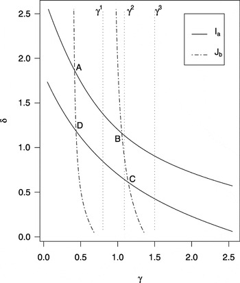
The construction of U(α_a,α_b) and L(α_a,α_b) is illustrated in Figure 1 generated from the Monte Carlo study in Section 3, which follows, in which γ and δ are scalars. The curves marked I_a denote the boundaries of the {I(α_a,γ)} regions, whereas the curves marked J_b denote the boundaries of the {J(α_b,δ)} regions. From (1) it follows that the K(α_a,α_b) region is given by the curved trapezoid ABCD; then from (2) and (3) it follows that γ¹ belongs to both U(α_a,α_b) and L(α_a,α_b), γ² belongs to U(α_a,α_b) but not to L(α_a,α_b), and γ³ belongs to neither U(α_a,α_b) nor L(α_a,α_b).

Construction of bounds confidence regions.

The difference between the procedure described here and that of Dufour (1990) is that the latter requires that the confidence regions for the nuisance parameters are marginal with respect to the parameters of interest, i.e., I(α,γ_a) = I(α,γ_b) for all 0 < α < 1 and all γ_a,γ_b ∈ Γ. In Figure 1 this would require that the I_a curves are horizontal straight lines for all realizations of the data.

THEOREM 1. Let α, α₁, α₂, and α₂′ be constants between 0 and 1 that satisfy

and let {I(α₁,γ);γ ∈ Γ}, {J(α₂,δ);δ ∈ Δ}, and {J(α₂′,δ);δ ∈ Δ} be systems of confidence regions for γ and δ such that

where (γ₀,δ₀) denote the true values of (γ,δ); then

where U(α₁,α₂) and L(α₁,α₂′) are defined as in (2) and (3).

Proof. The proof is based on the proofs of Propositions 1 and 2 from Dufour (1990). First, observe that

by the intersection rule and (4). From (1) and (2) it follows that (γ,δ) ∈ K(α₁,α₂) implies that γ ∈ U(α₁,α₂) so that Pr{γ₀ ∈ U(α₁,α₂)} ≥ Pr{(γ₀,δ₀) ∈ K(α₁,α₂)}. This combined with (7) verifies the first inequality in (5).

Second, for any 0 < α_a,α_b < 1 define

and then observe that

using (4). But the complement of L(α₁,α₂′) is given by

and thus Pr{γ₀ ∈ L(α₁,α₂′)^c} ≥ Pr{γ₀ ∈ Q(α₁,α₂′)} ≥ α so that Pr{γ₀ ∈ L(α₁,α₂′)} ≤ (1 − α), which verifies the second inequality in (5).

Third, note that because J(α₂′,δ) ⊆ J(α₂,δ) for all δ ∈ Δ then K(α₁,α₂′) ⊆ K(α₁,α₂) and hence L(α₁,α₂′) ⊆ L(α₁,α₂). From (2) and (3) it is clear that L(α₁,α₂) ⊆ U(α₁,α₂), and together these imply (6). █

There are several points to note about this procedure. First, there is no guarantee that the resulting regions will always be nonempty. Indeed, the definitions of U(α₁,α₂) and L(α₁,α₂′) given by (2) and (3) specifically permit the possibility that I(α₁,γ) may be empty for certain values of γ. If I(α₁,γ) is empty for a given value of γ then it follows from (2) and (3) that this value of γ belongs neither to U(α₁,α₂) nor to L(α₁,α₂′). Second, the procedure can be swapped around to construct bounds confidence regions for δ provided that I(α_a,γ) ⊆ I(α_b,γ) for all γ ∈ Γ and α_a ≥ α_b. Third, if there exists a system of exact confidence regions {I*(α)} for δ such that I(α,γ) = I*(α) irrespective of the value of γ then this procedure for constructing confidence regions for γ is the same as that introduced by Dufour (1990) whenever I*(α) is nonempty. Last, as in Dufour (1990), the requirement of constructing a confidence region for the nuisance parameters can be avoided by setting α₁ = 0 and α₂ = α₂′ = α, thus leading to a particularly simple version of the confidence region for the parameters of interest because Δ is always a valid choice for I*(0).

As in Dufour (1990), a rather tighter pair of bounds confidence regions is available when the events δ₀ ∈ I(α_a,γ₀) and γ₀ ∈ J(α_b,δ₀) are independent for any choices of 0 < α_a,α_b < 1.

THEOREM 2. Let α, α₁, α₂, and α₂′ be constants between 0 and 1 that satisfy

and let {I(α₁,γ);γ ∈ Γ}, {J(α₂,δ);δ ∈ Δ}, and {J(α₂′,δ);δ ∈ Δ} be systems of confidence regions for γ and δ such that conditions (i) and (ii) from Theorem 1 are satisfied and that the events δ₀ ∈ I(α_a,γ₀) and γ₀ ∈ J(α_b,δ₀) are independent for any choice of 0 < α_a,α_b < 1, where (γ₀,δ₀) denote the true values of (γ,δ). Then (5) and (6) hold.

Proof. The proof is almost identical to that of Theorem 1. The independence assumption together with (12) implies that the derivation in (7) can be replaced by

whereas that in (10) can be replaced by

The rest of the proof follows exactly the same lines as that of Theorem 1. █

3. DEPENDENT VARIABLE HETEROSKEDASTICITY

In this section we apply the procedure for constructing exact bounds confidence regions to a dependent variable heteroskedasticity (DVH) model. This is a useful example because there are no obvious exact marginal confidence regions for the nuisance parameters other than useless ones based on unrelated randomization. Thus the approach adopted by Dufour (1990) and by Dufour and Kiviet (1996) cannot be applied directly.

The DVH model has received a moderate amount of attention in the econometrics literature (Amemiya, 1973; Battese and Bonyhady, 1981; Prais, 1953; Prais and Houthakker, 1955; Theil, 1951, 1971). In the standard DVH model the dependent variables are independent normal random variables whose expectations are linear functions of the exogenous variables and whose variances are proportional to the squares of their expectations. We consider the case where there are two exogenous variables and where the disturbances are independent normals, i.e.,

where μ_t(β) = β₁ x_1t + β₂ x_2t, the {x_1t} and {x_2t} are nonstochastic, β⁰ = (β₁⁰,β₂⁰)′, β₁⁰ and β₂⁰ are unknown constants, and σ₀² is an unknown positive constant. For convenience we assume that μ_t(β⁰) > 0 for all t = 1,…,T and restrict attention to the region B = {β : μ_t(β) > 0 for all t = 1,…,T}. The problem is to construct confidence regions for β₂.

In what follows it is useful to work with the artificial regression equation

where z_t(β) = (y_t − μ_t(β))/μ_t(β), w_jt(β) = x_jt /μ_t(β), ρ_j(β) = (β_j⁰ − β_j) for j = 1,2, and η_t(β) = u_t /μ_t(β). Note that ρ₁(β⁰) = ρ₂(β⁰) = 0 and η_t(β⁰) ∼ IN(0,σ₀²). We can write (16) in matrix form as z(β) = W(β)ρ(β) + η(β), with ρ(β⁰) = 0 and η(β⁰) ∼ N [0,σ₀²I_T] . Now define H₀¹(β) as the hypothesis that ρ₁(β) = 0 and ρ₂(β) = 0, H_A¹(β) as the hypothesis that ρ₁(β) ≠ 0 but ρ₂(β) = 0, H₀²(β) as the hypothesis that ρ₂(β) = 0, and H_A²(β) as the hypothesis that ρ₂(β) ≠ 0, all within the artificial regression (16). Clearly, H₀¹(β⁰) and H₀²(β⁰) both hold.

Let

denote the usual F-statistic for testing H₀^j(β) against H_A^j(β) in (16) for j = 1,2. When β = β⁰ then (16) becomes a normal classical linear regression model with all its regression coefficients equal to zero. Consequently

has an exact central F-distribution with (1,T − 1) degrees of freedom whereas

has an exact central F-distribution with (1,T − 2) degrees of freedom. In addition, because both H₀¹(β⁰) and H_A¹(β⁰) are nested within H₀²(β⁰) then

is independent of

(Gourieroux, Monfort, and Vuong, 1995, p. 181). The {I(α_a,β₂)} and {J(α_b,β₁)} systems of confidence regions are then constructed as

where c_r,s(α) is the usual α significance level critical value for an F-test with (r,s) degrees of freedom. Because

and

are independent and c_r,s(α) is a monotonically decreasing function of α it follows that these systems of confidence regions satisfy the conditions of Theorem 2.

For the Monte Carlo study we set β₁⁰ = β₂⁰ = 1 and σ₀² = 0.09. We considered sample sizes of T = 25, 50, 100, and 200. For each value of T we set x_1t = 1 for all t and generated the {x_2t} as the absolute values of T independent N(1,4) random variables. We then generated 1,000 replications keeping the {x_2t} fixed across the replications for a given value of T. To construct the confidence regions for β₂ we used a discrete parameter space consisting of a 251 × 251 evenly spaced grid with steps of 0.01 from 0.05 to 2.55 for both β₁ and β₂. We then set α = 0.10, α₁ = 0.05, α₂ = 0.05263, and α₂′ = 0.10526 to focus on 90% confidence regions: it is easy to verify that these choices satisfy the conditions of Theorem 2.

Figure 1 in Section 2 illustrates the {I(α_a,β₂)} and {J(α_b,β₁)} systems of confidence regions constructed in this manner with α_a = 0.05 and α_b = 0.10526 for a particular realization with T = 25; here γ is used to denote β₂ and δ to denote β₁. In this particular realization the J_b curves that denote the right and left boundaries of the {J(α_b,β₁)} regions are quite close to being vertical except for very low values of β₁, for which they curve somewhat to the right as β₁ decreases. In contrast, the I_a curves that denote the upper and lower boundaries of the {I(α_a,β₂)} regions curve noticeably downward as β₂ increases. The calculations for this realization were done in Ox version 2.20 (Doornik, 1999) on a Pentium III 450 MHz personal computer and took 27 seconds. The graphs were generated using the R programming language (Ihaka and Gentleman, 1996).²

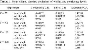
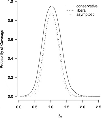
Figure 2 shows the empirical probabilities of coverage at different values of β₂ when β₁⁰ = β₂⁰ = 1, σ₀² = 0.09, and T = 25. As can be seen, the probabilities of coverage at different values of β₂ for the asymptotic and liberal confidence regions are very similar, whereas those of the conservative confidence region are noticeably higher. This is supported by Table 1, which shows the mean widths, the standard deviations of the widths, and empirical confidence levels for the conservative, liberal, and asymptotic confidence regions (C.R.s). The empirical confidence levels of the asymptotic regions tend to be slightly higher than the nominal 10% value, but the differences may simply be the result of Monte Carlo sampling variability (and might well be negligible under a suitable degrees of freedom adjustment to the asymptotic critical values). Table 1 also shows that the mean widths of the various regions are roughly inversely proportional to the sample size, though interestingly the standard deviations of the widths diminish much more rapidly with the sample size. This may be due to the reduction in the variability of the estimator of σ² as the sample size grows.

Mean widths, standard deviations of widths, and confidence levels

Probabilities of coverage at different values of β2 for β10 = β20 = 1, σ2 = 0.09, and T = 25.

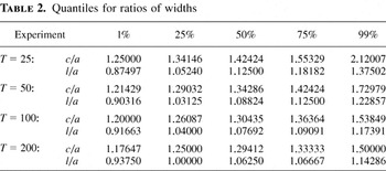
Table 2 shows the quantiles for the ratios of the widths of the conservative and liberal confidence regions to the width of the asymptotic confidence region (c/a and l/a, respectively). These show that the conservative confidence region is essentially always wider than the asymptotic confidence region whereas the liberal confidence region is often, but not always, wider than the asymptotic confidence region. In addition, as the sample size increases the dispersion in the relative widths decreases. Overall the results indicate that the asymptotic and liberal confidence regions perform quite similarly in this situation.

Quantiles for ratios of widths