Implications
If the current trend in the demand for milk and beef remains at the same level in Germany and other European countries, a holistic approach will be required to evaluate whether increasing milk yield per cow is a valid strategy to mitigate greenhouse gas (GHG) emissions. The approach used in this study accounts for GHG emissions associated not only with milk production, but also with beef production. This study shows that if both milk and beef production are to remain constant, considerably increasing milk yield per cow could result in higher GHG emissions.
Introduction
Increasing milk yield per cow in dairy farms has been proposed as one strategy to reduce greenhouse gas (GHG) emissions in agriculture, as less cows are needed to produce the same amount of milk (Monteny et al., Reference Monteny, Bannink and Chadwick2006; Steinfeld and Wassenaar, Reference Steinfeld and Wassenaar2007; Smith et al., Reference Smith, Martino, Cai, Gwary, Janzen, Kumar, McCarl, Ogle, O'Mara, Rice, Scholes, Sirotenko, Howden, McAllister, Pan, Romanenkov, Schneider, Towprayoon, Wattenbach and Smith2008). As methane (CH4) from enteric fermentation contributes to approximately 50% of total GHG emissions in dairy farms (Hörtenhuber et al., Reference Hörtenhuber, Lindenthal, Amon, Markut, Kirner and Zollitsch2010), reducing the number of cattle seems to be the main strategy to reduce GHG emissions. CH4 emissions related to milk yield (g CH4/kg milk) decline as milk yield per cow increases (Flachowsky and Brade, Reference Flachowsky and Brade2007). However, the strategy of increasing milk yield per cow to mitigate GHG emissions is focused only on emissions related to milk production, and therefore, it does not consider the amount of GHG emissions associated with beef production as a co-product. If a constant demand for beef is to be met, the loss of beef production due to less dairy cows has to be compensated for by increasing the number of suckler cows (Martin and Seeland, Reference Martin and Seeland1999).
The quota system for milk production in the European Union (EU), including Germany, together with the continuous increase in milk yield per cow have resulted in less total dairy cows producing a similar total amount of milk, with a reduced amount of beef produced as a co-product of the dairy system (von Witzke and Noleppa, Reference Von Witzke and Noleppa2010). In the season 1999 to 2000, the 27 EU member countries (EU-27) had a net trade (export minus import) of 0.37 million tons of bovine meat and a net trade of 2.3 million tons of dairy products. By the season 2008 to 2009, although dairy products’ net trade remained relatively constant (2.2 million tons), the EU-27 changed from being a net exporter to a net importer of 0.15 million tons of bovine meat (Eurostat, 2010). Thus, self-sufficiency for beef decreased from 104% in 1999 to 98% in 2008 (Weiß and Kohlmüller, Reference Weiß and Kohlmüller2010).
Cederberg and Stadig (Reference Cederberg and Stadig2003) estimated that approximately 50% of European beef production is a co-product of the dairy sector. In Germany, approximately 70% of total beef production can be considered a co-product of the dairy sector (own calculations according to Weiß and Kohlmüller, Reference Weiß and Kohlmüller2010). Milk yield per cow per year has increased from 6700 to 9300 kg in the United States and from 4900 to 6600 kg in Germany between 1990 and 2009 (Food and Agriculture Organization of the United Nations Statistics (FAOSTAT), 2010). With increasing milk yield per cow, milk and beef production tend to be more independent. High specialization of milk and beef production can be observed in the United States where the share of beef cows of total cows is approximately 78% (United States Department of Agriculture (USDA), 2010). However, in some regions of the world, such as Southern Germany, Austria and Switzerland, beef production as a co-product of the dairy sector still plays an important role, with dual-purpose cows as a key component.
The objective of this study was to determine the effect of increasing milk yield per cow on total GHG emissions, land use and economic performance for German dairy systems under two different scenarios: constant milk but decreased beef output (Scenario 1); and constant milk and beef output (Scenario 2). The originality of this study comes from its holistic approach, which integrates dairy and beef production to estimate GHG emissions.
Material and methods
Model overview
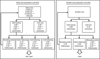
A model was developed, using MSExcel®, to estimate the effects of increasing milk yield per cow on GHG emissions and on side effects such as milk and beef production, feeding costs, type of land use and labour. The model incorporates several animal production systems for milk and beef production, as well as the cultivation of agricultural land needed to provide feed to the animals. The model makes all calculations based on production units (PUs) to connect milk and beef production. Two types of PU were defined (Figure 1), namely dairy cow PU (DU) and suckler cow PU (SU). A DU is defined as a dairy cow that produces milk and beef. Beef production comes not only from cull cows but also from fattening of surplus heifers, bulls and cull calves. Three types of DU were simulated by changing the breed and the level of milk yield as follows:
Diagrammatic representation of the dairy cow production unit (DU) and the suckler cow production unit (SU). Calves per cow per year were calculated taking into account assumptions for calving interval and calf losses due to diseases of 8%; the same number of stars means that the animals belong to the same production unit.

(i) Milk yield of 6000 kg/cow per year using dual-purpose Fleckvieh (FV) cows (DU-6).
(ii) Milk yield of 8000 kg/cow per year using dual-purpose FV cows (DU-8).
(iii) Milk yield of 10 000 kg/cow per year using Holstein–Friesian (HF) cows (DU-10).
Assumptions for milk and beef production in the model were chosen to represent typical German production systems. Average recorded milk yield of German dairy cows in 2009 was 7980 kg milk/cow per year (Arbeitsgemeinschaft Deutscher Rinderzüchter (ADR), 2010). Thus, the three types of cows simulated represent the average situation of milk yield per cow per year in Germany (8000 kg), a situation with lower milk yield than the average (6000 kg milk/cow per year) representing average dual-purpose dairy cows and a situation with greater milk yield (10 000 kg milk/cow per year) than the average, representing HF dairy herds. It is assumed that all surplus calves from DU-6 and DU-8 are fattened as bulls or heifers, whereas 50% of bull calves from DU-10 were assumed to be fattened as calves, given the breeds used in each case.
As shown in Figure 1, SU includes the suckler cow and the associated animal categories: heifer rearing, bull and heifer fattening. FV was chosen as the breed for the modelled SU, because it is one of the most important breeds for suckler cow production systems in Germany. Beef output from culled cows, bulls and heifers fattening is calculated for the SU.
Production and management data used in the model
Animal production
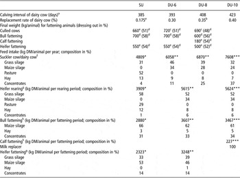
Management and production assumptions for the modelled PU are shown in Table 1. Higher replacement rates for higher yielding dairy cows were assumed, in order to account for the higher replacement rate reported for systems with higher milk yield per cow per year (Lucy, Reference Lucy2001; Dillon et al., Reference Dillon, Berry, Evans, Buckley and Horan2006). Age at first calving was set at 27 months for all replacement heifers included in the model.
Production and management assumptions considered for the modelled animals

SU = suckler cow production unit; DU = dairy cow production unit.
aHaenel (Reference Haenel2010).
bADR (2010).
cHaiger and Knaus (Reference Haiger and Knaus2010).
dLandeskuratorium der Erzeugerringe für tierische Veredelung in Bayern unpublished results.
eKTBL (2008).
fIncluding calf rearing till *270 to 290 kg; **85 kg; *** 50 kg.
gInitial weight heifer rearing/fattening: * 270 kg, ** 85 kg, *** 50 kg.
hInitial weight bull/calf fattening: * 290 kg, ** 85 kg, ***50 kg.
Dairy cows, replacement heifers, bulls and heifers for fattening were assumed to be indoor all-year-round. Forage composition for all modelled dairy cows was set to represent a common German feeding system (Kuratorium für Technik und Bauwesen in der Landwirtschaft (KTBL), 2008), with 50% grass silage, 40% maize silage and 10% hay. Total dry matter intake (DMI) and the proportion of concentrates in dairy cows ration were calculated in order to satisfy requirements for metabolizable energy and crude protein (CP; Gesellschaft für Ernährungsphysiologie (GfE), 2001), accounting for limitation on DMI (Gruber et al., Reference Gruber, Pries, Spiekers, Schwarz and Staudacher2006). The equation used to predict DMI was built and validated by Gruber et al. (Reference Gruber, Pries, Spiekers, Schwarz and Staudacher2006), using a data set comprising 2264 dairy cows from different research institutes and breeds in Germany, Austria and Switzerland. Gruber et al.'s (Reference Gruber, Pries, Spiekers, Schwarz and Staudacher2006) equation takes into account the following parameters: breed, country, live weight, milk yield, amount of concentrates fed, metabolizable energy content of forage and the ratio of CP to energy in the diet. Feed rations for calf and heifer rearing, suckler cows, bull and heifer fattening were calculated to satisfy required CP and metabolizable energy (GfE, 1995 and 2001) based on common German production systems (Deutsche Landwirtschafts-Gesellschaft (DLG), 2005; KTBL, 2008) (Table 1). Suckler cows and associated replacement heifers were assumed to be on pasture for 185 days/year from mid-April to mid-October and were housed in straw-based systems for the rest of the year.
Concentrate composition for all modelled animals was assumed to be made up of wheat, barley and soyabean meal. For the 10 000 kg yielding dairy cow, corn was supplemented as a slow digestible carbohydrate.
It is assumed that surplus male and female calves from modelled FV dairy cows (6000 and 8000 kg yielding dairy cows) are passed to bull and heifer fattening at a weight of 85 kg, and calves from the modelled HF dairy cow (10 000 kg yielding dairy cow) at a weight of 50 kg, representing German production systems (Brüggemann, Reference Brüggemann2011).
Forage and crop production
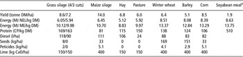
Model assumptions used for forage and crop production are shown in Table 2. Feed quality values were taken from DLG feed tables (DLG, 1997). Information about quantities of lime, pesticide, seed and diesel input used in forage and crop production (Bayerische Landesanstalt für Landwirtschaft (LfL), 2006; KTBL, 2008) were necessary for the calculation of GHG emissions and are shown in Table 2.
Production and management assumptions considered for the modelled feed production

DM = dry matter; NEL = net energy lactation; ME = metabolizable energy.
aaverage yield of soyabeans during 2004 to 2008 from USA, Brazil, Argentina (FAOSTAT, 2010); characteristics of soybeans: 87% DM, 20.8% oil (Dalgaard et al., Reference Dalgaard, Schmidt, Halberg, Christensen, Thrane and Pengue2008).
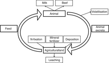
The nitrogen (N) cycle plays an important role in the calculation of GHG emissions in cattle production systems. On the one hand, excreted N can be used as fertilizer for forage and crop production, which in turn reduces the amount of purchased mineral fertilizer. On the other hand, it is a source of direct (manure storage, N2O emissions from soils due to manure input) and indirect (ammonia volatilization and nitrate leaching) N2O emissions (Olesen et al., Reference Olesen, Schelde, Weiske, Weisbjerg, Asman and Djurhuus2006). N content in animals’ excreta was calculated according to DLG (2005). Thus, excreta-N was calculated as the difference between N intake from forage and concentrates and N retained as animal products (i.e. milk and live weight gain). The available manure from animals was assumed to be applied on the land used for forage and crop production according to ‘good agricultural practice’ (LfL, 2007) with the exception of land used for soyabean meal production as soyabean meal was assumed to be imported. In the forage and crop production areas, a soil N balance was calculated as the difference between N inputs (manure application, deposition and fixation) and N output (N in the crop harvested, losses through nitrate leaching and ammonia volatilization) (Figure 2). N fixation was assumed to be 50 kg N/ha per year for grassland-3 cuts, hay and pasture, and 30 kg N/ha per year for grassland-4 cuts. The N required to equalize inputs and outputs was assumed to be added as mineral fertilizer. Phosphate and potassium balance were calculated using a similar procedure to the N balance.
Diagrammatic representation of the nitrogen (N) cycle incorporated in the model

Economic calculations for the costs of forage production were mainly based on data from LfL (2006) and KTBL (2008). Full cost accounting includes all variable and fixed costs of average German forage production. Prices for wheat, barley, corn and soyabean meal were 132 €/tonne, 128 €/tonne, 141 €/tonne and 257 €/tonne, respectively, based on 5-year average market prices (2005 to 2009; Schaack et al., Reference Schaack, von Schenck and Schraa2010).
Calculation of GHG emissions
Calculations of GHG emissions in the model were made for primary and secondary sources of CH4, N2O and CO2 emissions. Primary sources of GHG emissions are those occurring on-farm during feed production, maintenance of animals and manure management. Secondary sources of GHG emissions include emissions occurring off-farm, for instance, those generated during production of fertilizer, pesticides or diesel (Rotz et al., Reference Rotz, Montes and Chianese2010). In order to standardize, all gases are expressed as CO2 equivalents (CO2eq). The global warming potential is calculated according to Intergovernmental Panel on Climate Change (IPCC, 2007), set at 25 kg CO2eq/kg of CH4 and 298 kg CO2eq/ kg of N2O (100-year horizon). Emissions from the production of capital goods such as buildings and machinery are not accounted for following recommendations from the British Standards Institution (BSI, 2008).
Primary source GHG emissions
Primary source emissions considered in the model comprise CH4 emissions from enteric fermentation, CH4 and N2O emissions from manure storage and N2O emissions related to N input introduced into the soil. Furthermore, CO2 emissions from liming and indirect N2O emissions from N leaching were included in the model. Indirect N2O emissions from ammonia volatilization were not included in the model.
Enteric fermentation
For dairy cows, CH4 emissions from enteric fermentation were predicted according to Kirchgeßner et al. (Reference Kirchgeßner, Windisch and Müller1995):

where ‘CH4’ is the CH4 release from dairy cows (g/day), ‘CF’ is the intake of crude fibre (kg/day), ‘NfE’ is the intake of N-free extract (kg/day), ‘CP’ is the intake of CP (kg/day) and ‘EE’ is the intake of ether extract (kg/day). For all other animals, CH4 emissions from enteric fermentation were predicted according to IPCC (2006, equation 10.21):

where ‘CH4ent’ describes enteric CH4 emissions (kg/animal per year), ‘GE’ is the intake of gross energy (MJ/animal per year); ‘η’ is the energy content of CH4 (55.65 MJ/kg CH4) and ‘x CH4’ is the CH4 conversion rate of feed energy to CH4 (MJ/MJ). CH4 conversion rate was assumed to be 0.065 for rearing and beef cattle and 0.02 for calves up to 125 kg live weight (Haenel, Reference Haenel2010).
Manure management
CH4 and N2O emissions from manure management occur mainly from liquid slurry and farmyard manure during storage. Standard barn and manure storage systems were assumed in the model according to KTBL (2008), with free stall barns with slatted floors for dairy cows and rearing heifers and boxes with slatted floors for bulls and heifers for fattening. Liquid slurry was stored in open slurry tanks. Calves were assumed to be bedded in straw-based systems until the weight of 125 kg. CH4 emissions from manure storage were calculated according to IPCC (2006, equation 10.23):

where ‘VS’ is the amount of volatile solids excreted (kg/animal per year); ‘Bo’ is the maximum CH4 production capacity (m3/kg CH4) and ‘MCF’ is the CH4 conversion factor. Volatile solids were calculated on the basis of digestibility of organic matter, GE of feed intake and ash content of manure (Haenel, Reference Haenel2010). The ash content of manure was assumed to be 0.08 kg/kg (IPCC, 2006). The ‘Bo’ was assumed to be 0.24 m3/kg CH4 for dairy cows and 0.18 m3/kg CH4 for all other modelled animals (Haenel, Reference Haenel2010). CH4 conversion factors of 0.1, 0.02 and 0.01 were used for slurry, farmyard manure and pasture excretion, respectively (Haenel, Reference Haenel2010). Calculations for N2O emissions from manure storage were based on N excretion and an emission factor 0.005 for solid storage and slurry (IPCC, 2006, equation 10.25).
Soil N2O and CO2 emissions
The N2O emissions from production of forages and crops (used to feed animals) are an important source of GHG emissions in animal production systems. Lovett et al. (Reference Lovett, Shalloo, Dillon and O'Mara2006) and Hörtenhuber et al. (Reference Hörtenhuber, Lindenthal, Amon, Markut, Kirner and Zollitsch2010) reported that N2O emissions from production of forages and crops represent up to 12% of total GHG emissions from Irish and Austrian dairy farms, respectively. The N2O emissions in this study were calculated on the basis of N input into the soil in the form of mineral fertilizer, manure and crop residues. A default emission factor of 0.01 kg N2O-N/kg N input was used for N2O emissions from all types of N input except N excretion of pasture cattle. Emissions due to animal excreta during grazing were calculated using an emission factor of 0.02 kg N2O-N/kg N excreted (IPCC, 2006).
Owing to leaching, 20 kg N/ha of grassland and 30 kg N/ha of arable land were assumed to be lost each year (LfL, 2007). The input of N into surface and ground waters give rise to indirect N2O emissions (Haenel, Reference Haenel2010). An emission factor of 0.0075 kg N2O-N/kg N input was used to calculate indirect N2O emissions from N leaching.
To avoid acidification, 150 kg CaO/ha grassland per year and 400 kg CaO/ha arable land per year were assumed to be applied (LfL, 2007). CO2 emissions due to liming were assumed to be 0.785 kg CO2/kg CaO input (Patyk and Reinhardt, Reference Patyk and Reinhardt1997). The emission factor from diesel consumption was set at 2.637 kg CO2eq/kg diesel (Rotz et al., Reference Rotz, Montes and Chianese2010).
Secondary source GHG emissions
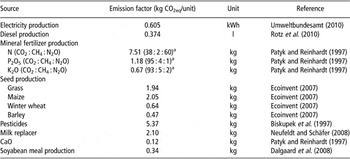
Emissions occurring during the production of electricity, diesel, mineral fertilizer, crop seeds and soyabean meal (which was assumed to be produced off-farm) were estimated and integrated into the model using the emission factors shown in Table 3. Electricity required for milking-related activities was set at 0.056 kWh/kg milk (Kraatz, Reference Kraatz2009), whereas electricity consumption for all other animals was calculated according to KTBL (2008). Inputs for diesel, seed, pesticide and lime consumption used in forage and crop production are shown in Table 2.
Emission factors for modelled second source greenhouse gas emissions

CO2eq = kg CO2 equivalents.
aThe data in brackets are percentages of total CO2eq.
Modelled scenarios
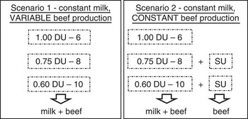
The influence of increasing milk yield per cow per year on GHG emissions and on other side effects was analysed under two scenarios. The first was designed to keep milk production constant (1 DU-6, 0.75 DU-8 and 0.60 DU-10) while increasing milk yield per dairy cow. This results in reduced beef production as a co-product (Figure 3; Scenario 1). The second was designed to keep milk and beef production constant, adding SU to compensate for the beef production lost as the number of cows is reduced with increasing milk yield per cow (Figure 3; Scenario 2).
Considered scenarios in the modelling (DU = dairy cow production unit; SU = suckler cow production unit – see Figure 1).

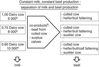
To determine GHG emissions per kg milk and per kg beef within Scenario 2 (constant beef), milk and beef production of the modelled PU were separated using different methods of co-product handling (Figure 4). A co-product of the dairy cow is beef from culled cows and surplus calves. According to International Organization for Standardization (ISO, 2006), different methods can be used to handle co-products when calculating GHG emissions. In this study, the ‘no allocation’ and the ‘economic allocation’ methods were used.
Separation of milk and beef production within Scenario 2. aincluding breeding heifer. bmethods for handling co-products from dairy cow production: ‘No allocation’: co-products are not loaded with GHG emissions from dairy cow production; ‘Economic allocation’: co-products are loaded with greenhouse gas (GHG) emissions from dairy cow production systems according to equation (4).

‘No allocation’ means that all emissions occurring in the process of milk production (GHG emissions from dairy cow including replacement heifer and rearing calves) were related to milk output (left side of Figure 4). Beef production includes beef from culled cows, beef from heifer and bull fattening and from suckler cow. As GHG emissions occurring in the dairy production system were not allocated between milk and co-products, beef from culled cows and calves for bull and heifer fattening were not loaded with GHG emissions. Thus, emissions per kg beef were those occurring during bull and heifer fattening and suckler cow production.
‘Economic allocation’ considers the value of milk and co-products (surplus calves and beef from culled cows). In the ‘economic allocation’ method, GHG emissions occurring in the process of milk production are allocated to milk and co-products according to their economic value using the following equation:

where em is the proportion of GHG emissions allocated to milk, pm is the price of milk (€/kg milk), am is the amount of milk (kg/year), pb is the price for beef from culled cows (€/kg beef), ab is the amount of beef from culled cows (kg/year), pc is the price for surplus calves (€/calf) and ac is the amount of surplus calves/year. Prices for milk (30.8 C t/kg milk), beef and surplus calves were calculated on the basis of a 5-year average of German statistical data (2005 to 2009; Wohlfahrt et al., Reference Wohlfahrt, Gorn, Hellebrand, Michels and Thielen2008; Gorn and Schoch, Reference Gorn and Schoch2010). In the ‘economic allocation’ method, the proportion of GHG emissions allocated to co-products is 1-em. Thus, emissions per kg beef include emissions allocated to beef from culled cows and calves derived from dairy cow production and emissions occurring during bull and heifer fattening and suckler cow production.
Results
Scenario 1: constant milk, variable beef production
GHG emissions
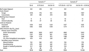
The DU-6 had a milk output of 5770 kg/year (4% of milk produced assumed to be used for calves, own consumption or wasted) and a beef output of 322 kg/year (Table 4). From total beef production, 34% came from culled dairy cow, and the remaining from heifer and bull fattening of surplus calves. Modelled GHG emissions per DU-6 included emissions derived from dairy cow, rearing heifer, bull and heifer fattening were 9578 kg CO2eq/year (Table 4). Estimated CH4 emissions from enteric fermentation and N2O emissions from N input into soils accounted for approximately 50% and 15% of total GHG emissions, respectively. GHG emissions, for a constant level of milk output and decreasing associated beef output, decreased from 9578 kg CO2eq (DU-6) to 6141 kg CO2eq/year (0.6 DU-10). As CH4 emissions from enteric fermentation accounted for approximately 50% of total GHG emissions, reduction in animal numbers influenced total GHG output considerably.
Model output for Scenarios 1 and 2

DU = dairy cow production unit; SU = suckler cow production unit; GHG = greenhouse gas; CO2eq = kg CO2 equivalents.
aScenario 1: constant milk production; variable beef production; model outputs refer to a constant level of 5770 kg milk.
bScenario 2: constant milk and constant beef; model outputs refer to a constant level of 5770 kg milk and 322 kg beef.
Milk and beef outputs
As milk yield per cow increased, the number of dairy cows required to keep milk output constant (5770 kg) declined. On the basis of the milk output of a DU-6, only 0.75 DU-8 and 0.60 DU-10 were needed to keep milk output constant. With increasing milk yield per cow, beef output decreased from 322 kg (DU-6) to 236 kg (0.75 DU-8) and to 131 kg/year (0.6 DU-10). This was the result of a decline in the number of both culled cows and fattening cattle, in addition to a less-efficient process of fattening for HF cattle. Ratio of milk to beef production (kg/kg) was 18 for DU-6, 25 for DU-8 and 44 for DU-10.
Land use, costs and labour
Demand for grassland decreased with increasing milk yield from 0.58 ha (DU-6) to 0.43 ha (0.75 DU-8) and 0.34 ha/year (0.6 DU-10), because of decreasing number of animals and a decreasing proportion of grass silage in the diet (Table 5). Demand for arable land (includes land used to produce maize silage, concentrates and soyabean meal of the animals rations) remained constant at 0.66 ha for DU-6 and 0.75 DU-8. However, demand for arable land decreased from 0.66 to 0.58 ha for 0.6 DU-10, as fattening of HF calves was included with a diet based on milk replacer (Table 4). Both costs for forage production and working hours decreased considerably as the milk yield per cow increased from 6000 kg to 10 000 kg/year, assuming constant milk output of 5770 kg/year (Table 4, Scenario 1). Assuming labour costs of 10 €/h, feed and labour costs decreased approximately 35%, with increasing milk yield from 6000 to 10 000 kg milk/cow per year, which would result in increasing profit with increasing milk yield/cow per year.
Modelled GHG emissions for Scenario 2

DC = dairy cow; GHG = greenhouse gas; CO2eq = kg CO2 equivalents; PU = production unit; SU = suckler cow production unit.
aAll GHG emissions occurring in dairy cow production and heifer rearing are allocated to milk.
bGHG emissions occurring during dairy cow production and heifer rearing are allocated to milk according to their economic value (equation 4); initial weight bull and heifer fattening: *85 kg; **50 kg.
Scenario 2: separation of constant milk and constant beef production.
Scenario 2: constant milk and constant beef production
The second scenario simulated was one with both milk and beef outputs constant. This was done by combining DU and SU. Milk and beef output were constrained at 5770 kg/year and 322 kg/year, respectively, based on one DU-6.
GHG emissions
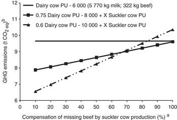
Total modelled GHG emissions were 9578 kg CO2eq for one DU-6, 9594 kg CO2eq for 0.75 DU-8 and 10 365 kg CO2eq for 0.6 DU-10, including SU in the two latter cases, assuming a constant amount of 5770 kg milk and 322 kg beef output (Table 4). The influence of increasing milk yield per cow on total GHG emissions in our study depended mainly on the amount of beef (as a co-product) that was compensated by beef production from suckler cows (Figure 5). The 10 000 kg yielding dairy cow resulted in the lowest GHG emissions up to a beef compensation rate of 68%. However, from a rate of beef compensation of 68% and 80% upwards, the DU-10 resulted in more GHG emissions than DU-8 and DU-6, respectively. The DU-8 showed similar GHG emissions as DU-6 at a rate of beef compensation of 100% (Figure 5).
Greenhouse gas (GHG) emissions resulting from different rates of compensation of missing beef by suckler cow production at a constant level of milk production (5770 kg); X: ranging from 0 to 0.27 SU for 0.75 DU-8 and from 0 to 0.59 SU for 0.6 DU-10. a100% compensation of missing beef means beef output is equal to 322 kg based on one DU 6000 kg milk/cow per year (see Figure 1). bThe amount of CO2eq refer to a constant amount of milk (5770 kg milk) and to a varying amount of beef indicated in the X-Ache (SU = suckler cow production unit; DU = dairy cow production unit).

Milk and beef outputs
With increasing milk yield per cow to 8000 and 10 000 kg/year, the inclusion of 0.27 and 0.59 SU were needed, respectively, to keep beef output constant at 322 kg/year (Figure 3 and Table 4).
Land use, costs and labour
As the diet of suckler cows was mainly based on grass, demand for grassland increased in the modelled scenario of constant milk production (one DU-6, 0.75 DU-8 and 0.60 DU-10) and constant beef production. In this scenario, in which suckler cows were included to keep beef output constant, demand for labour remained nearly constant and demand for total land increased (Table 4; Scenario 2). Within Scenario 2, DU-8000 kg (plus SU) showed the lowest demand for labour and the lowest feeding costs.
Scenario 2: constant milk and beef production – allocation methods
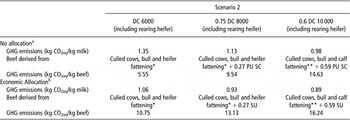
In order to show the impact of increasing milk yield per cow on GHG emissions per kg milk and per kg beef, milk and beef production of the modelled PU in Scenario 2 were separated using different methods of co-product handling (Figure 4), namely ‘no allocation’ and ‘economic allocation’.
No allocation
Using the ‘no allocation method’, emissions of 1.35 kg CO2eq/kg milk and 5.55 kg CO2eq/kg beef for DU-6 were estimated. With increasing milk yield per cow and year, GHG emissions per kg of milk decreased from 1.35 to 1.13 and 0.98 kg CO2eq as milk yield per cow increased from 6000 to 8000 and 10 000 kg milk, respectively. However, beef produced from suckler cows (to compensate for the decline of beef produced as co-product) as a proportion of total beef production increased with increasing milk yield per cow. Therefore, emissions per kg of beef output increased from 5.55 kg CO2eq (DU-6, with no beef from suckler cow production) to 14.63 kg CO2eq/kg beef output (0.6 DU-10, 59% of beef derived from suckler cow production; Table 5).
Economic allocation
The ‘Economic allocation’ method allocates GHG emissions from dairy cow production between milk and co-products according to their economic value. This resulted in lower GHG emissions per kg of milk but higher GHG emissions per kg of beef for the modelled scenarios in comparison with the ‘no allocation’ method (Table 5). ‘Economic allocation’ resulted in 10.75 kg CO2eq/kg beef for DU-6. GHG emissions per kg of beef increased in comparison with emissions estimated with ‘no allocation’, as beef from culled cows and calves for fattening were loaded with GHG emissions from milk production using the ‘economic allocation’ method. Calves from HF dairy cows (DU-10) were less valuable than calves from FV cows (DU-6 and DU-8). Thus, when ‘economic allocation’ was performed, more GHG emissions were allocated to milk for the 10 000 kg yielding dairy cow than for the other modelled dairy cows.
For both allocation methods, GHG emissions per kg milk decreased with increasing milk yield; however, the reduction of GHG emissions per kg milk was much higher within the ‘no allocation’ method than within the ‘economic allocation’ method. From dairy cow 8000 kg milk/year (including heifer) to dairy cow 10 000 kg milk/year (including heifer), GHG emissions decreased 0.15 kg CO2eq/kg milk using the ‘no allocation’ method and 0.04 kg CO2eq/kg milk using the ‘economic allocation’ method.
Discussion
The main objective of this study was to investigate the effect of increasing milk yield per cow on GHG emissions and on other side effects, not stopping at the dairy farm gate but looking at the whole system of milk and beef outputs. Two scenarios were defined: constant milk production (one DU-6, 0.75 DU-8 and 0.60 DU-10) and decreasing beef production, as milk yield per cow increased (Scenario 1); and both milk and beef production constant, by compensating the decline of beef production as co-products with beef production from suckler cows (Scenario 2).
Model limitations
GHG emissions
There is still a high uncertainty associated with equations and emission factors used to predict GHG emissions in agriculture (IPCC, 2006). Thus, further model calculations were carried out replacing equation 4 (equation to predict CH4 emissions from dairy cows) and emission factors used in this model (N2O emissions from N input into the soil) to see the effect on results shown in Table 4. Two additional equations predicting CH4 emissions from dairy cows were tested – an equation derived from Schils et al. (Reference Schils, Verhagen, Haarts, Kuikman and Sebek2006) considering different diet compositions and an equation described in IPCC (2006, equation 10.21). Total GHG emissions increased by up to 7% when these two equations were used in comparison with the modelled scenarios shown in Table 4. However, it did not change the trend towards a decrease in GHG emissions for Scenario 1 and the trend towards an increase in GHG emissions for Scenario 2, as milk yield per cow increased. Furthermore, emission factors of 0.01 kg N2O-N/kg N and 0.02 kg N2O-N/kg N for the prediction of direct N2O emissions from managed soils were replaced by the uncertainty range given in IPCC (2006) (0.003 to 0.3 and 0.007 to 0.6, respectively). Total GHG emissions shown in Table 4 decreased by up to 10% using the lower emission factors and increased by up to 38%, including the higher emission factors into the model. Again, this did not affect the relative trend observed for the modelled scenarios shown in Table 4.
Hindrichsen et al. (Reference Hindrichsen, Wettstein, Machmuller and Kreuzer2006) reported higher CH4 emissions from slurry of dairy cows offered forage supplemented with concentrates in comparison with dairy cows offered a forage-only diet. This is not considered in the IPCC (2006, equation 10.23) used in the model. If this was considered, it would result in slightly higher GHG emissions for higher-yielding dairy cows.
General model assumptions
Model assumptions as breed of dairy and suckler cows, calving interval, replacement rate and feeding system are based on typical German production systems. A change in breed for suckler cows could increase fattening efficiency of bulls (ADR, 2010) and heifers and result in less suckler cows needed to replace beef reduction in the model. A change in the feeding system of fattening bulls from forage based on maize silage to pasture could decrease daily gains and increase the number of suckler cows. Furthermore, assumptions of calving interval and replacement rate influence the number of calves per cow available for fattening and thus beef output considerably.
The influence of model assumptions and uncertainty of GHG emission factors on model outputs have to be taken into account while interpreting GHG emissions of the modelled scenarios. However, the overall conclusion that increasing milk yield in dairy farming could result in higher GHG emissions, if the whole system of milk and beef production is considered, remains.
Beef as a co-product of dairy cow production in Germany
In the model, DU was built to combine milk and beef production. The tight connection between milk and beef production can be observed in German development of milk and beef production in recent years. Milk yield per cow per year in Germany increased by approximately 2000 kg (4900 to 6600 kg milk/cow per year) from 1990 to 2009 (FAOSTAT, 2010). In the same period, the number of dairy cows in Germany decreased from approximately 6.3 to 4.2 million animals (Destatis, 2010), whereas total milk output remained constant. Owing to this decrease, gross domestic beef production in Germany declined by approximately 967 million kg in the same period (Destatis, 2010), which represents a 44% reduction of total beef production in Germany. This did not remarkably affect self-sufficiency of beef in Germany as beef demand has considerably decreased because of bovine spongiform encephalopathy (BSE) crises in 2001. However, as beef demand remained constant since 2002, self-sufficiency of beef decreased from 140% in 2002 to 117% in 2009 (Weiß and Kohlmüller, Reference Weiß and Kohlmüller2010).
Effect of market demand of milk and beef on model assumptions
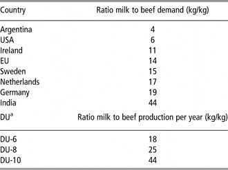
The extent to which increasing milk yield per cow reduces or increases GHG emissions depends on the demand for milk and beef as well as the ratio of milk to beef output per dairy cow. The ratio of milk (excluding butter) to beef consumption (kg/kg) in Germany was 18 for the year 2007 (FAOSTAT, 2010). This means that milk consumption exceeded beef consumption by more than 18 times. The ratio of milk to beef output per year (kg/kg) for the modelled DU was 18 for one DU-6, 25 for one DU-8 and 44 for one DU-10 (Table 6). Thus, if total milk demand in Germany is satisfied by dairy cows yielding 8000 kg of milk/year, beef demand cannot be satisfied by co-products of dairy cow production. Therefore, suckler cows will be needed for beef production. The ratio of milk to beef consumption of a given country together with the ratio of milk to beef production (as co-product) from dairy cows are the most important factors in defining whether increasing milk yield per cow is a valid strategy to reduce total GHG emissions in that country.
Ratio of milk to beef demand for several countries (FAOSTAT, 2010) and ratio of milk to beef production for the modelled dairy cow production units

aDU = dairy cow production unit differing in milk yield per cow per year (6000 kg (DU-6), 8000 kg (DU-8) and 10 000 kg (DU-10)).
Considering international trade and influence of future suppression of quota system in Europe on milk production of certain countries, it is also important to consider the ratio of milk to beef demand of other countries. The ratio of milk to beef production for modelled DU exceeds the ratio of milk to beef demand in many countries and in the EU, with the exception of Germany and India (Table 6). Thus, the reduction of beef production due to increasing milk yield per cow would result in a higher number of suckler cows if the ratio of milk to beef demand remains at the present level. If, along with an increasing milk yield per cow, there is a corresponding decrease in beef consumption (towards a higher ratio of milk to beef demand) and an increase in pork and poultry meat consumption, reductions in beef output would not have to be compensated for by an increasing number of suckler cows. Emissions per kg meat from pork (6.4 kg CO2eq/kg meat) or poultry (4.6 kg CO2eq/kg meat) production systems (Williams et al., Reference Williams, Audsley and Sandars2006) are assumed to be much lower than emissions per kg beef from suckler cow production (21.2 kg CO2eq/kg meat, own calculations; 21.7 kg CO2eq/kg meat, Beauchemin et al., Reference Beauchemin, Janzen, Little, McAllister and McGinn2010). In this case, total GHG emissions (from milk and meat production) will be reduced as milk yield per cow is increased.
Furthermore, it has to be considered that the quality of beef derived from specialized suckler cow production could be higher than the quality of beef derived from co-products of dairy cow production and thus influence quality of beef offer. Offer and demand for high-quality beef was not analysed in this study and further research needs to consider this.
Allocation methods
Most studies calculating GHG emissions from dairy farming stop at the dairy farm gate (Lovett et al., Reference Lovett, Shalloo, Dillon and O'Mara2006; Hörtenhuber et al., Reference Hörtenhuber, Lindenthal, Amon, Markut, Kirner and Zollitsch2010), using different methods for allocating GHG emissions between milk and co-products. In our study, milk and beef production were combined defining PU and including suckler cow production in the model. Within Scenario 2 (constant milk and beef output), GHG emissions for the modelled PU were also allocated between milk and beef output using different methods of co-product handling, to determine emissions per kg milk and per kg beef. Results showed that emissions per kg beef were 4 to 18 times higher than emissions per kg milk, depending on milk yield per cow and allocation method.
Results showed that the method of handling co-products influences the amount of GHG emissions per kg of milk and per kg of beef produced. If only emissions per kg milk were considered, GHG emissions decreased with increasing milk yield per cow in both allocation methods used in this study. However, GHG emissions per kg beef produced increased considerably as milk yield per cow increased. Thus, calculations of GHG emissions that stop at the dairy farm gate are not always adequate to represent the whole impact of cattle production systems on GHG emissions.
Another approach to handle co-products of dairy farming that considers suckler cows is ‘system expansion’ (defined in Cederberg and Stadig, Reference Cederberg and Stadig2003). Using this method, suckler cow production is defined as an alternative way to replace co-product of dairy farming (beef from culled cows and surplus calves). However, in comparison with the approach in this study, the ‘system expansion’ method does not consider the fattening systems of surplus calves and does not account for differences in breed. In the ‘system expansion’ method, surplus calves from a dairy cow are replaced by calves from suckler cow production; however, it does not take into account that calves of dual-purpose breed show better fattening characteristics than calves of specialized dairy breeds. In the current model, the definition of PU included the dairy cow, replacement heifer and bull and heifer fattening from surplus dairy cow calves. Thus, differences derived from both level of milk production and breeds were taken into account.
Side effects of increasing milk yield per cow
Loss of fertility and higher probability of the appearance of diseases are mentioned as side effects of increasing milk yield per cow in dairy farming (Lucy, Reference Lucy2001; Dillon et al., Reference Dillon, Berry, Evans, Buckley and Horan2006). GHG emissions produced during the rearing phase of modelled replacement heifers contribute up to 20% of total GHG emissions from the modelled dairy farms. Thus, replacement rate plays an important role in total GHG emissions of dairy systems. Weiske et al. (Reference Weiske, Vabitsch, Olesen, Schelde, Michel, Friedrich and Kaltschmitt2006) reported a reduction of GHG emissions per kg milk by up to 13% with a reduction of replacement rate from 40% to 30% for modelled dairy farms. However, if a constant beef production is assumed (Scenario 2), changing the assumed replacement rate of the 10 000 kg-yielding dairy cow from 40% to 30% did not reduce total GHG emissions. In this scenario, a reduction in replacement rate resulted in less beef from culled cows and thus a higher amount of beef to be replaced by suckler cows.
In this study, with increased milk yield per cow, the proportion of concentrates and soyabean meal in the ration fed to dairy cows increased, whereas the demand for grassland area decreased. This change in the diet has a side effect on GHG emissions, as demand for additional arable land may influence clearance of land elsewhere (Garnett, Reference Garnett2009). Cultivation of soyabean in South America is often assumed to be associated with the conversion of forest, pasture and shrub land to cropland. Dalgaard et al. (Reference Dalgaard, Schmidt, Halberg, Christensen, Thrane and Pengue2008) reported 5.7 kg CO2eq/kg soyabean meal if land use changes are included in the calculation of GHG emissions. Calculating GHG emissions with the emission factor of 5.7 kg CO2eq/kg soyabean meal, total GHG emissions of Scenario 2 (constant milk and constant beef production) increased 25%, 31% and 32% for DU-6, 0.75 DU-8 including SU and 0.6 DU-10 including SU, respectively. This resulted in a higher increase of GHG emissions with increasing milk yield within Scenario 2.
As demand for grassland decreases with increasing milk yield per cow, the proportion of human-edible feed sources in the ration increases. Monogastric livestock systems are more efficient in terms of total feed conversion efficiency (kg cereals consumed/kg animal weight gain; Garnett, Reference Garnett2009). However, efficiencies of energy and protein on the basis of human-edible food produced per unit of human-edible feed consumed per animal are higher for ruminants than for monogastric animals (Gill et al., Reference Gill, Smith and Wilkinson2010). In this study, concentrate intake per dairy cow increased with increasing milk yield from 11% to 25% and 37% of total DMI for the 6000, 8000 and 10 000 kg milk-yielding dairy cows, respectively. Thus, higher-yielding dairy cows had a higher input of human-edible food. Human-edible efficiency (output human-edible protein/dairy cow per input human-edible protein) was 1.05 for a dairy cow yielding 6000 kg milk per year, 0.68 for a dairy cow yielding 8000 kg milk per year and 0.55 for a dairy cow yielding 10 000 kg milk per year. Output included milk and beef/cow per year with a protein content of 190 g/kg beef, and 3.4%/kg milk input included protein content of concentrates feed per cow per year.
The introduction of suckler cow production increased GHG emissions in the present model estimations because of the high emission factors/kg beef produced. Again, it has to be mentioned that feed input for suckler cow production is mainly derived from non-human-edible sources (forage and hay). Furthermore, suckler cows can be farmed on less valuable land, with other ecosystem services such as conservation of biodiversity, water quality and aesthetic value.
Conclusion
In response to the original question in this paper ‘Does increasing milk yield per cow reduce GHG emissions?’, the answer would be yes, if GHG emissions are measured per kg milk yield and reduction in associated beef production is not accounted for. However, model outputs showed that this would not be the case if beef production is intended to be constant and milk yield per cow increases. Thus, the whole impact of increasing milk yield per cow in dairy farming on GHG emissions, and on other side effects, can only be observed by expanding the system boundaries from the dairy farm gate to the whole system to consider both milk and beef production. Regarding the modelled GHG efficiency, the ongoing specialization in both milk and beef production has to be questioned.
The extent to which total GHG emissions increase with increasing milk yield per cow also depends on the amount of beef that has to be compensated for and on the kind of meat (beef, pork or poultry) that compensates beef reduction as a co-product from dairy cows.
Further research is needed to determine how a change in the ratio of milk to beef demand and the demand for high-quality beef would influence model outputs.
Acknowledgement
The corresponding author gratefully acknowledges the financial support given by the Association for Technology and Structures in Agriculture (Kuratorium für Technik und Bauwesen in der Landwirtschaft).