1 Introduction
As the demand for air traffic grows, there is a great need for new techniques and methods by which the emissions of aircraft can be reduced. One of the ways to achieve this is to suppress flow separation and thus reduce the friction drag, which comprises more than 50 % of the total drag on an aircraft (Schrauf Reference Schrauf2005). This can either be done through a proper wing and nacelle design that enables a naturally laminar flow over the surfaces to be maintained, or via manipulation of the flow through active or passive control devices. A classical approach to control transition and separation is through boundary layer suction. Suction causes the boundary layer velocity profile to become fuller and more stable, which implies that it has a higher critical Reynolds number and is susceptible to a smaller range of unstable disturbances. This also means that it generates a thinner boundary layer with a higher local skin friction (Schlichting Reference Schlichting1979). However, due to the large differences between the skin friction of a laminar and a turbulent boundary layer, the total effect of suction is favourable. In order to limit the complexity of the system, suction is often combined with natural laminar flow (NLF) design, by which the extent of the suction surface may be reduced to a smaller portion of the wing close to the leading edge. This approach is termed hybrid laminar flow control (HLFC) (Joslin Reference Joslin1998).
An ideal suction surface consists of a continuously permeable surface that enables the wall-normal velocity to attain a non-zero value on the wall (Gregory Reference Gregory and Lachmann1961). However, a porous skin approximating such a surface have proven to be impractical for a number of reasons, and experiments have shown that it is possible to obtain laminar flow by instead applying suction through discrete holes positioned in regular patterns at different positions along the chord (Gregory & Walker Reference Gregory and Walker1955). In the vicinity of a discrete suction perforation, the flow is strongly three-dimensional and features locally inflectional velocity profiles, streamwise vortices and for closely spaced perforations horseshoe vortices that bridge neighbouring perforations (Meyer Reference Meyer1955; Gregory Reference Gregory1962; Meitz & Fasel Reference Meitz and Fasel1994; MacManus & Eaton Reference MacManus and Eaton1996, Reference MacManus and Eaton1998, Reference MacManus and Eaton2000). Behind each perforation, a pair of streamwise counter-rotating vortices develop that is connected to a pair of counter-rotating vortices inside the suction pipe (Gregory Reference Gregory and Lachmann1961; MacManus & Eaton Reference MacManus and Eaton2000). Their strengths depend on the ratio
 $R$
between the suction velocity and the free-stream velocity, as well as on the hole diameter to displacement thickness ratio,
 $d^{\ast }/\unicode[STIX]{x1D6FF}_{h}^{\ast }$
(MacManus & Eaton Reference MacManus and Eaton1996). The level of streamwise vorticity is typically highest at the suction perforation and decreases rapidly with downstream distance (Meitz & Fasel Reference Meitz and Fasel1994; MacManus & Eaton Reference MacManus and Eaton1996). However, as the lateral separation between the vortices tend to grow behind the perforation, interaction of vortices generated at neighbouring perforations may in some cases increase the vorticity again further downstream due to lift-up and stretching (Meitz & Fasel Reference Meitz and Fasel1994).
Given a pair of streamwise vortices in the aft of a suction perforation, streaks form in the boundary layer. These structures may eventually destabilise and cause transition. Experiments have reported that for one row of perforations, the transition position increases linearly with the suction ratio at a rate roughly independent on the free-stream velocity
 $U_{\infty }^{\ast }$
, until a critical suction ratio
 $R_{crit}$
is exceeded and the transition point moves forward abruptly – a phenomenon referred to as oversuction. An increase in free-stream velocity has further been noted to have an adverse effect on
 $R_{crit}$
, but by using several rows of perforations, the transition position and
 $R_{crit}$
may generally be increased relative to the single row configuration (Butler Reference Butler1955). Regarding the variation of
 $R_{crit}$
with spanwise hole spacing
 $s^{\ast }/d^{\ast }$
,
 $R_{crit}$
seems to have a local minimum around
 $s^{\ast }/d^{\ast }=2.67$
for a single row of perforations. Below this point the critical suction ratio increases sharply as the holes seemingly behave like a spanwise slot, and above this the critical suction ratio increases gradually as the holes become isolated (Butler Reference Butler1955; Gregory & Walker Reference Gregory and Walker1955; Gregory Reference Gregory and Lachmann1961). For multiple rows of perforations, this minimum of
 $R_{crit}$
is displaced towards larger
 $s^{\ast }/d^{\ast }$
ratios (Gregory & Walker Reference Gregory and Walker1955). A diagram illustrating the relationship between
 $R_{crit}$
and the hole diameter
 $d^{\ast }/\unicode[STIX]{x1D6FF}_{h}^{\ast }$
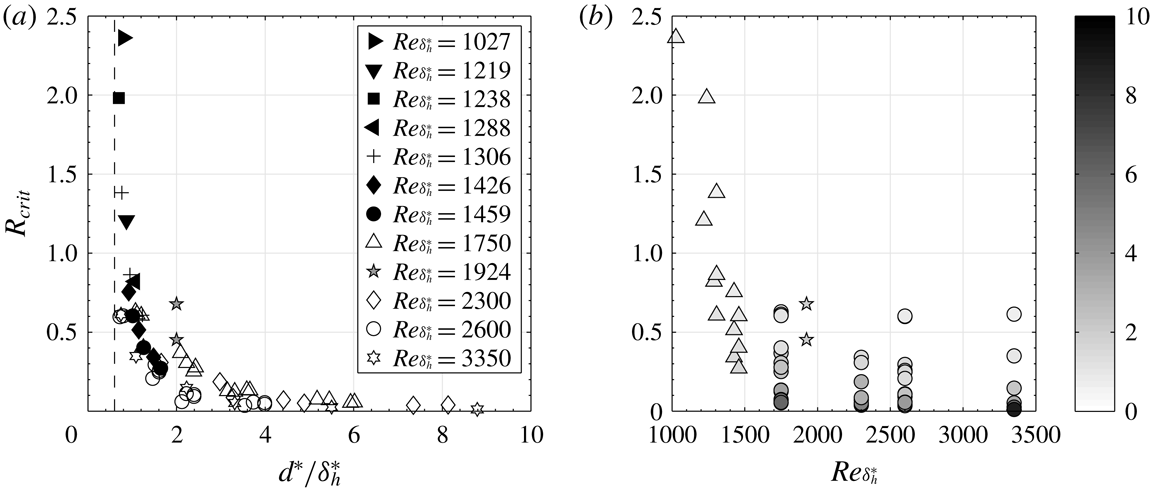
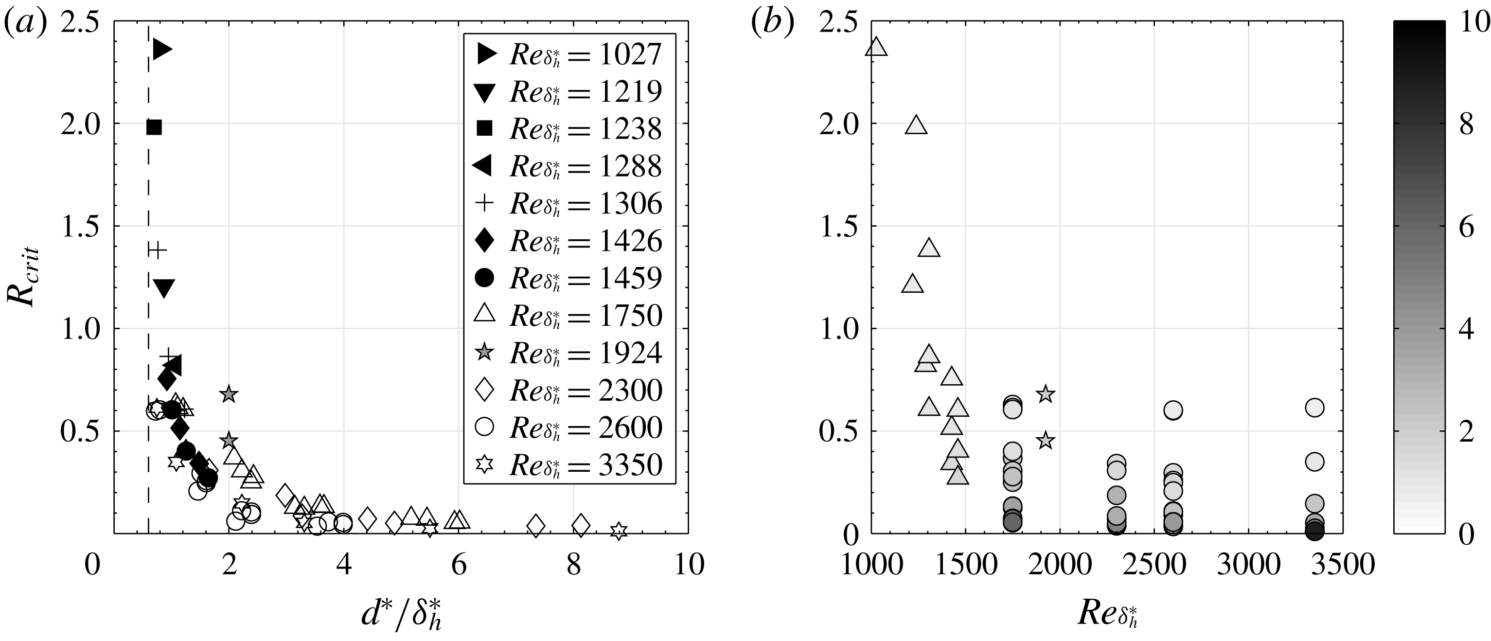
was compiled by MacManus & Eaton (Reference MacManus and Eaton1998, Reference MacManus and Eaton2000) (see figure 1
a). Their diagram suggests that these parameters are approximately inversely proportional to each other, where
 $R_{crit}$
goes to zero for large
 $d^{\ast }/\unicode[STIX]{x1D6FF}_{h}^{\ast }$
and increases sharply as
 $d^{\ast }/\unicode[STIX]{x1D6FF}_{h}^{\ast }$
approaches 0.6 from above. For
 $d^{\ast }/\unicode[STIX]{x1D6FF}_{h}^{\ast }\lesssim 0.6$
, a critical
 $R$
need not exist at all.
(a) Variation of the critical suction ratio
 $R_{crit}$
with
 $d^{\ast }/\unicode[STIX]{x1D6FF}_{h}^{\ast }$
for different
 $Re_{\unicode[STIX]{x1D6FF}_{h}^{\ast }}$
, adapted from MacManus & Eaton (Reference MacManus and Eaton1998, Reference MacManus and Eaton2000). The open symbols correspond to transonic measurements by Blanchard et al. (Reference Blanchard, Seraudie, Breil and Payry1991), and the slightly sub- and supercritical suction ratios investigated in the present study are marked with grey pentagrams (✩). The limiting value
 $d^{\ast }/\unicode[STIX]{x1D6FF}_{h}^{\ast }=0.6$
is marked with a dashed line. (b) The data in (a) are replotted to show the variation of
 $R_{crit}$
with
 $Re_{\unicode[STIX]{x1D6FF}_{h}^{\ast }}$
. The symbols are shaded according to
 $d^{\ast }/\unicode[STIX]{x1D6FF}_{h}^{\ast }$
and correspond to the measurements by MacManus & Eaton (Reference MacManus and Eaton1998, Reference MacManus and Eaton2000) (▵), Blanchard et al. (Reference Blanchard, Seraudie, Breil and Payry1991) (○) and the present study (✩).
For the boundary layer with localised suction, the transition often begins by instabilities in the streamwise vortices (Meitz & Fasel Reference Meitz and Fasel1994; MacManus & Eaton Reference MacManus and Eaton1998, Reference MacManus and Eaton2000; Müller Reference Müller2012). To predict and circumvent these, various design criteria have been suggested. Some with the aim to propose limiting values for, e.g.
 $d^{\ast }/\unicode[STIX]{x1D6FF}_{h}^{\ast }$
,
 $s^{\ast }/d^{\ast }$
and row number that yield laminar flow up to a certain free-stream velocity (Gregory & Walker Reference Gregory and Walker1955). Others have noted that the effect on the flow of a suction hole in certain aspects is similar to that of a localised roughness element, and hence tried to invent criteria for transition prediction that are similar to those already existing in the roughness literature (see Gregory Reference Gregory and Lachmann1961, MacManus & Eaton Reference MacManus and Eaton1998, Reference MacManus and Eaton2000 and the references therein). These criteria have recently been reviewed and discussed by Müller (Reference Müller2012).
Despite of all these investigations, the origin of the reported premature transition remains unclear. Butler (Reference Butler1955) suggested that the occurrence of
 $R_{crit}$
could arise due to cyclic variations of surface pressure in the spanwise direction, as a result of the row of suction perforations. Such pressure variations that are normal to the free stream would presumably result in unstable secondary velocity profiles that eventually break down. Gregory (Reference Gregory and Lachmann1961) proposed that since each vorticity line that crosses a perforation gets sucked into it and the line segment outside of the perforation becomes stretched as it is advected downstream, an increase in suction ratio would strengthen the trailing vortex pair, which upon surpassing a certain limit would become unstable (see MacManus & Eaton Reference MacManus and Eaton2000 for a discussion on this). Meitz & Fasel (Reference Meitz and Fasel1994) put forth the hypothesis that for closely spaced holes, the instability could either begin in the vortices or in the recirculation region that forms between the vortices. MacManus & Eaton (Reference MacManus and Eaton1998, Reference MacManus and Eaton2000) observed the development of turbulent wedges around the trailing longitudinal vortices, and conjectured that the instability were initiated on the conical surfaces surrounding the vortex cores.
This fundamental question is of major importance for successful implementation of HLFC. A better understanding of the physical mechanisms and flow structures involved in the transition process may not only lead to better understanding of the receptivity process, but to improved design criteria for laminar wings and suction systems. To address this issue, a three-dimensional stability analysis accompanied by direct numerical simulations (DNS) and a Koopman analysis is peformed.
The structure of the article is as follows. In § 2, the set-up along with the numerical methods considered are described. The results of the analysis are given in § 3, including an account of the characteristic flow structures observed, the results from the linear stability and sensitivity analysis and finally a comparison between the linear and the nonlinear dynamics. The article concludes in § 4 with a discussion of the reported findings.
2 Computational set-up and methodology
2.1 Flow configuration and numerical method
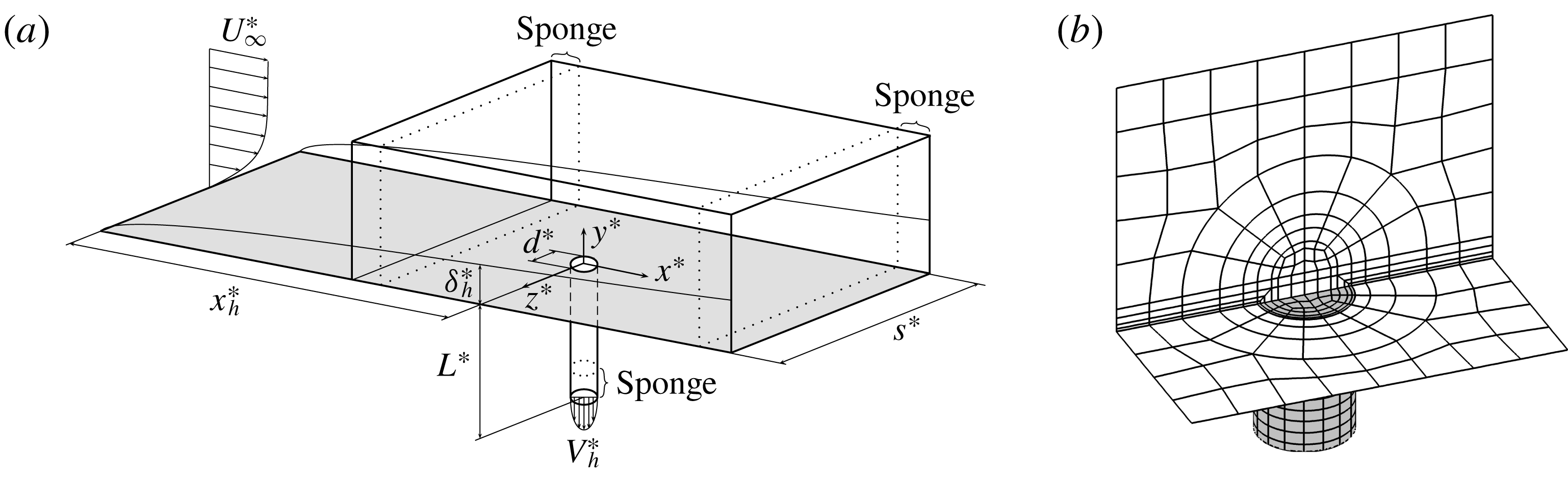
A sketch of the computational set-up is shown in figure 2(a) and consists of a rectangular box with the extents
 $[-34,125]\times [0,15]\times [-15,15]$
(in units of the displacement thickness
 $\unicode[STIX]{x1D6FF}_{h}^{\ast }$
) in the
 $x$
-,
 $y$
- and
 $z$
-directions, and a circular pipe mounted at the origin. In the past, some studies e.g. Meitz & Fasel (Reference Meitz and Fasel1994), have chosen to disregard the pipe in their computational set-up and replace it with a suitable Dirichlet boundary condition on the wall. However, since the vortices developing in the boundary layer have been found to be connected with the pipe orifice (MacManus & Eaton Reference MacManus and Eaton2000), and the velocity profile at the pipe inlet be very different from a Gaussian or a parabolic profile (Müller Reference Müller2012), neglecting the pipe may yield erroneous conclusions regarding the origin of the instability. This has been explicitly investigated for the related flow case ‘jet in cross-flow’ by Peplinski, Schlatter & Henningson (Reference Peplinski, Schlatter, Henningson, Fröhlich, Kuerten, Geurts and Armenio2015). In that study it was found that replacing a Dirichlet boundary condition consisting of a Gaussian velocity profile with a pipe destabilised the flow significantly, i.e. reduced the critical velocity ratio.
(a) Sketch of the numerical set-up (not drawn to scale) with the defining parameters. (b) Close-up of the mesh structure around the pipe orifice. Note that only the spectral element borders are shown and not the actual grid points.
Throughout the article, dimensional quantities are denoted with a superscript star, and quantities at the centre of the hole with a subscript
 $h$
. Velocities are made dimensionless with the free-stream velocity
 $U_{\infty }^{\ast }$
, and lengths with the unperturbed displacement thickness at the position of the hole
 $\unicode[STIX]{x1D6FF}_{h}^{\ast }$
(i.e. at the origin). The incompressible Blasius boundary layer subject to localised suction is determined by five independent dimensionless variables, namely, the boundary layer Reynolds number
 $Re_{\unicode[STIX]{x1D6FF}_{h}^{\ast }}=U_{\infty }^{\ast }\unicode[STIX]{x1D6FF}_{h}^{\ast }/\unicode[STIX]{x1D708}^{\ast }$
, the suction ratio (i.e. the velocity ratio) herein defined as the ratio between the suction centre line velocity and the free-stream velocity
 $R=|V_{h}^{\ast }|/U_{\infty }^{\ast }$
, the ratio between the diameter of the pipe and the displacement thickness at the pipe position
 $d^{\ast }/\unicode[STIX]{x1D6FF}_{h}^{\ast }$
, the spanwise hole spacing to diameter ratio
 $s^{\ast }/d^{\ast }$
and the ratio between the length and the diameter of the pipe
 $L^{\ast }/d^{\ast }$
. (Note, however, that if
 $L^{\ast }/d^{\ast }$
is chosen sufficiently large so that the flow in the pipe becomes fully developed, the influence of this parameter vanishes.) In the simulations performed, the dimensionless variables
 $d=d^{\ast }/\unicode[STIX]{x1D6FF}_{h}^{\ast }=2$
,
 $s=30$
(
 $s^{\ast }/d^{\ast }=15$
),
 $L=40$
(
 $L^{\ast }/d^{\ast }=20$
) and
 $Re_{\unicode[STIX]{x1D6FF}_{h}^{\ast }}=1924$
will be fixed, and
 $R$
will be varied. With this spanwise spacing the holes will act as isolated (see figure 10 in Butler Reference Butler1955 or figure 10a in Gregory Reference Gregory and Lachmann1961). The hole is positioned a distance
 $x_{h}^{\ast }/\unicode[STIX]{x1D6FF}_{h}^{\ast }=649.73$
from the leading edge so that the Reynolds number based on the streamwise position and the free-stream velocity reads
 $Re_{x_{h}^{\ast }}=1.25\times 10^{6}$
. It is emphasised that although this Reynolds number is above the critical value for Tollmien–Schlichting (TS) waves, no such perturbations are considered in the present work. For a detailed account of the TS instability, the reader is referred to Schmid & Henningson (Reference Schmid and Henningson2001).
The flow is described by the time-dependent incompressible Navier–Stokes equations subject to constant fluid properties
 $$\begin{eqnarray}\displaystyle & \displaystyle \frac{\unicode[STIX]{x2202}\boldsymbol{u}}{\unicode[STIX]{x2202}t}+\boldsymbol{u}\boldsymbol{\cdot }\unicode[STIX]{x1D735}\boldsymbol{u}=-\unicode[STIX]{x1D735}p+\frac{1}{Re_{\unicode[STIX]{x1D6FF}_{h}^{\ast }}}\unicode[STIX]{x1D6FB}^{2}\boldsymbol{u}+\boldsymbol{f}\quad \text{in }\unicode[STIX]{x1D6FA}, & \displaystyle\end{eqnarray}$$
 $$\begin{eqnarray}\displaystyle & \displaystyle \unicode[STIX]{x1D735}\boldsymbol{\cdot }\boldsymbol{u}=0\quad \text{in }\unicode[STIX]{x1D6FA}, & \displaystyle\end{eqnarray}$$
 $\boldsymbol{u}=(u,v,w)^{\text{T}}$
denotes the velocity components in the
 $x$
-,
 $y$
- and
 $z$
-directions (see figure 2
a for the coordinate system adopted), and
 $\unicode[STIX]{x1D6FA}$
is the flow domain. At the inflow boundary the Blasius profile is specified (Schlichting Reference Schlichting1979), at the outflow boundary a stress-free condition is prescribed
 $Re_{\unicode[STIX]{x1D6FF}_{h}^{\ast }}^{-1}\unicode[STIX]{x2202}u/\unicode[STIX]{x2202}x-p=0$
,
 $Re_{\unicode[STIX]{x1D6FF}_{h}^{\ast }}^{-1}\unicode[STIX]{x2202}v/\unicode[STIX]{x2202}y=0$
,
 $Re_{\unicode[STIX]{x1D6FF}_{h}^{\ast }}^{-1}\unicode[STIX]{x2202}w/\unicode[STIX]{x2202}z=0$
, on the free-stream boundary a modified stress-free condition is used
 $u=U_{\infty }$
,
 $Re_{\unicode[STIX]{x1D6FF}_{h}^{\ast }}^{-1}\unicode[STIX]{x2202}v/\unicode[STIX]{x2202}y-p=0$
,
 $w=0$
and in the spanwise direction periodic conditions are assigned. At the end of the suction pipe, a laminar parabolic velocity profile is prescribed
 $V_{pipe}(r)=-R(1-r^{2})$
with
 $r=\sqrt{x^{2}+z^{2}}$
.
The term
 $\boldsymbol{f}$
in (2.1) represents a volume force containing the sponge term
 $\unicode[STIX]{x1D6FE}(x,y)(\boldsymbol{u}_{Bl-p}-\boldsymbol{u})$
. (The subscript ‘Bl–p’ refers to a velocity field that satisfies the Blasius similarity solution in the boundary layer and gives a parabolic profile inside the pipe.) The sponge is added next to the inflow and outflow as sketched in figure 2(a) to smoothly dampen perturbations and diminish boundary reflections. Application of the sponge region next to the inflow thus ensures that there are no disturbances in the boundary layer upstream of the suction hole. The sponge function is defined as
 $$\begin{eqnarray}\displaystyle & \displaystyle \unicode[STIX]{x1D6FE}(x,y)=\unicode[STIX]{x1D6FE}_{max}\left[S\left(\frac{x-x_{start}}{\unicode[STIX]{x1D6E5}_{rise}}\right)+S\left(\frac{x_{end}-x}{\unicode[STIX]{x1D6E5}_{fall}}\right)+S\left(\frac{y_{end}-y}{\unicode[STIX]{x1D6E5}_{fall}}\right)\right], & \displaystyle\end{eqnarray}$$
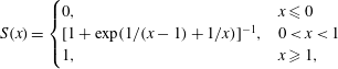 $$\begin{eqnarray}\displaystyle & \displaystyle S(x)=\left\{\begin{array}{@{}ll@{}}0,\quad & x\leqslant 0\\ \hspace{0.0pt}[1+\exp (1/(x-1)+1/x)]^{-1},\quad & 0<x<1\\ 1,\quad & x\geqslant 1,\end{array}\right. & \displaystyle\end{eqnarray}$$
 $\unicode[STIX]{x1D6FE}_{max}=1$
,
 $\unicode[STIX]{x1D6E5}_{rise}=18.75$
and
 $\unicode[STIX]{x1D6E5}_{fall}=6.75$
. The length of the sponge is
 $\unicode[STIX]{x1D6E5}_{length}=34$
, and
 $x_{start}$
and
 $x_{end}$
are chosen such that the sponge is divided proportionally to
 $\unicode[STIX]{x1D6E5}_{rise}$
and
 $\unicode[STIX]{x1D6E5}_{fall}$
between the outflow and the inflow. The variable
 $y_{end}$
is chosen so that the sponge region inside the pipe has the same length as that next to the inflow. With these parameters the extents of the domain outside the sponge region are
 $-25\leqslant x\leqslant 100$
(
 $-25\leqslant x\leqslant 140$
for mesh M3) and
 $-31\leqslant y\leqslant 15$
.
All computations have been performed with the high-order DNS code Nek5000 (Fischer, Lottes & Kerkemeier Reference Fischer, Lottes and Kerkemeier2008), which is based on the spectral element method (SEM) (Patera Reference Patera1984). Within the SEM, the Navier–Stokes equations are solved in weak form and the fluid domain is decomposed into hexahedral elements, wherein the velocities are represented by tensor products of one-dimensional
 $N$
th-order Lagrange interpolants on the Gauss–Lobatto–Legendre quadrature points. The pressure is in turn represented by tensor products of one-dimensional
 $(N-2)$
th-order Lagrange interpolants on the Gauss–Legendre quadrature points, following
 $\mathbb{P}_{N}$
–
 $\mathbb{P}_{N-2}$
(Maday & Patera Reference Maday, Patera and Noor1989).
Overview of the different domains and meshes used in the study. The dimensions of the domains are specified as
 $[x_{min},x_{max}]\times [y_{min},y_{max}]\times [z_{min},z_{max}]$
in units of
 $\unicode[STIX]{x1D6FF}_{h}^{\ast }$
.

Details and extents of the different meshes used here are given in table 1. The mesh M1 is the one used for most of the study, whereas mesh M2 and M3 are aimed at verifying that the flow is sufficiently resolved and that the results are independent of the domain length, respectively. The mesh structure is visualised in figure 2(b). The pipe is joined to the boundary layer box through a hemispherical cap that reduces the effect of the pipe junction on the mesh structure inside the box.
2.2 Linear stability analysis
To investigate the linear stability of the flow, the flow quantities are decomposed into a steady component and a perturbation according to
 $\boldsymbol{u}=\boldsymbol{U}+\unicode[STIX]{x1D716}\boldsymbol{u}^{\prime }$
and
 $p=P+\unicode[STIX]{x1D716}p^{\prime }$
, where
 $\unicode[STIX]{x1D716}$
is a small parameter. By substituting these decompositions into (2.1) and equating terms with the same order of
 $\unicode[STIX]{x1D716}$
, a set of equations for the base flow and the linear evolution of the perturbation is obtained.
2.2.1 Base flow
The equations governing the base flow are similar to (2.1) and read
 $$\begin{eqnarray}\displaystyle & \displaystyle \frac{\unicode[STIX]{x2202}\boldsymbol{U}}{\unicode[STIX]{x2202}t}+\boldsymbol{U}\boldsymbol{\cdot }\unicode[STIX]{x1D735}\boldsymbol{U}=-\unicode[STIX]{x1D735}P+\frac{1}{Re_{\unicode[STIX]{x1D6FF}_{h}^{\ast }}}\unicode[STIX]{x1D6FB}^{2}\boldsymbol{U}+\boldsymbol{F}\quad \text{in }\unicode[STIX]{x1D6FA}, & \displaystyle\end{eqnarray}$$
 $$\begin{eqnarray}\displaystyle & \displaystyle \unicode[STIX]{x1D735}\boldsymbol{\cdot }\boldsymbol{U}=0\quad \text{in }\unicode[STIX]{x1D6FA}. & \displaystyle\end{eqnarray}$$
 $-\unicode[STIX]{x1D712}(\boldsymbol{U}-\bar{\boldsymbol{U}})$
to the volume force
 $\boldsymbol{F}$
that corresponds to a differential low-pass filter
 $$\begin{eqnarray}\frac{\unicode[STIX]{x2202}\bar{\boldsymbol{U}}}{\unicode[STIX]{x2202}t}=\frac{\boldsymbol{U}-\bar{\boldsymbol{U}}}{\unicode[STIX]{x1D6E5}}.\end{eqnarray}$$
The filter dampens temporal oscillations in the velocity field above its cutoff frequency and forces the flow towards a steady solution
 $\bar{\boldsymbol{U}}$
. The method requires two calibration parameters: a filter width
 $\unicode[STIX]{x1D6E5}$
related to the cutoff frequency as
 $\unicode[STIX]{x1D714}_{c}=1/\unicode[STIX]{x1D6E5}$
, and a control coefficient
 $\unicode[STIX]{x1D712}$
related to the filter gain. These parameters are related to the frequencies and the growth rates of the instabilities in the flow and are chosen as
 $\unicode[STIX]{x1D6E5}=42/\unicode[STIX]{x03C0}$
and
 $\unicode[STIX]{x1D712}=0.3$
.
2.2.2 Eigenvalue problem
The linearised Navier–Stokes equations describing the evolution of the perturbation read
 $$\begin{eqnarray}\displaystyle & \displaystyle \frac{\unicode[STIX]{x2202}\boldsymbol{u}^{\prime }}{\unicode[STIX]{x2202}t}+\boldsymbol{u}^{\prime }\boldsymbol{\cdot }\unicode[STIX]{x1D735}\boldsymbol{U}+\boldsymbol{U}\boldsymbol{\cdot }\unicode[STIX]{x1D735}\boldsymbol{u}^{\prime }=-\unicode[STIX]{x1D735}p^{\prime }+\frac{1}{Re_{\unicode[STIX]{x1D6FF}_{h}^{\ast }}}\unicode[STIX]{x1D6FB}^{2}\boldsymbol{u}^{\prime }+\boldsymbol{f}^{\prime }\quad \text{in }\unicode[STIX]{x1D6FA}, & \displaystyle\end{eqnarray}$$
 $$\begin{eqnarray}\displaystyle & \displaystyle \unicode[STIX]{x1D735}\boldsymbol{\cdot }\boldsymbol{u}^{\prime }=0\quad \text{in }\unicode[STIX]{x1D6FA}, & \displaystyle\end{eqnarray}$$
 $\boldsymbol{f}^{\prime }=-\unicode[STIX]{x1D6FE}(x,y)\boldsymbol{u}^{\prime }$
. To investigate the sensitivity of the flow, the adjoint of (2.5) will be considered as well,
 $$\begin{eqnarray}\displaystyle & \displaystyle -\frac{\unicode[STIX]{x2202}\boldsymbol{u}^{\dagger }}{\unicode[STIX]{x2202}t}-(\boldsymbol{U}\boldsymbol{\cdot }\unicode[STIX]{x1D735})\boldsymbol{u}^{\dagger }+(\unicode[STIX]{x1D735}\boldsymbol{U})^{\text{T}}\boldsymbol{u}^{\dagger }=-\unicode[STIX]{x1D735}p^{\dagger }+\frac{1}{Re_{\unicode[STIX]{x1D6FF}_{h}^{\ast }}}\unicode[STIX]{x1D6FB}^{2}\boldsymbol{u}^{\dagger }+\boldsymbol{f}^{\dagger }\quad \text{in }\unicode[STIX]{x1D6FA}, & \displaystyle\end{eqnarray}$$
 $$\begin{eqnarray}\displaystyle & \displaystyle \unicode[STIX]{x1D735}\boldsymbol{\cdot }\boldsymbol{u}^{\dagger }=0\quad \text{in }\unicode[STIX]{x1D6FA}, & \displaystyle\end{eqnarray}$$
 $\boldsymbol{f}^{\dagger }=-\unicode[STIX]{x1D6FE}(x,y)\boldsymbol{u}^{\dagger }$
. (Details of the derivation can be found in Barkley, Blackburn & Sherwin Reference Barkley, Blackburn and Sherwin2008.) Homogeneous Dirichlet boundary conditions are used for
 $\boldsymbol{u}^{\prime }$
and
 $\boldsymbol{u}^{\dagger }$
on all boundaries except in the spanwise direction, where periodicity is imposed. In order to satisfy such Dirichlet conditions, similar sponge regions as in the nonlinear simulations are used.
By assuming that the flow evolves in a divergence-free space, the perturbation equation (2.5) can be expressed in operator form as
 $$\begin{eqnarray}\frac{\unicode[STIX]{x2202}\boldsymbol{u}^{\prime }}{\unicode[STIX]{x2202}t}=\mathscr{L}\boldsymbol{u}^{\prime },\end{eqnarray}$$
with a similar expression for (2.6). Upon discretising (2.7) with the SEM and introducing the ansatz function
 $\boldsymbol{u}^{\prime }=\hat{\boldsymbol{u}}\text{e}^{-\text{i}\unicode[STIX]{x1D714}t}$
, where
 $\hat{\boldsymbol{u}}=(\hat{u} ,\hat{v},{\hat{w}})^{\text{T}}\in \mathbb{C}^{3}$
and
 $\unicode[STIX]{x1D714}\in \mathbb{C}$
, the following generalised eigenvalue problem is obtained
 $$\begin{eqnarray}-\text{i}\unicode[STIX]{x1D714}\unicode[STIX]{x1D648}\hat{\boldsymbol{u}}=\unicode[STIX]{x1D647}\hat{\boldsymbol{u}}.\end{eqnarray}$$
The discrete operators
 $\unicode[STIX]{x1D648}$
and
 $\unicode[STIX]{x1D647}$
in this equation represent the spectral element mass matrix and the discretised linearised Navier–Stokes operator, respectively. The eigenvalue problem (2.8) is solved using the implicitly restarted Arnoldi method, which is implemented in the P_ARPACK-library (Maschhoff & Sorensen Reference Maschhoff, Sorensen, Waśniewski, Dongarra, Madsen and Olesen1996; Lehoucq, Sorensen & Yang Reference Lehoucq, Sorensen and Yang1998). Instead of directly acting on a vector with the operator
 $\unicode[STIX]{x1D648}^{-1}\unicode[STIX]{x1D647}$
(or a subroutine performing the action of this operator), the system is integrated
 $\unicode[STIX]{x0394}t$
time units with a time stepper, which realises the action of the matrix exponential
 $\unicode[STIX]{x1D63D}(\unicode[STIX]{x0394}t)=\exp (\unicode[STIX]{x0394}t\unicode[STIX]{x1D648}^{-1}\unicode[STIX]{x1D647})$
. Given an initial random vector
 $\boldsymbol{u}_{0}^{\prime }$
, the algorithm generates an
 $m$
-dimensional Krylov space
 $$\begin{eqnarray}{\mathcal{K}}_{m}=\text{span}\{\boldsymbol{u}_{0}^{\prime },\unicode[STIX]{x1D63D}(\unicode[STIX]{x0394}t)\boldsymbol{u}_{0}^{\prime },\ldots ,\unicode[STIX]{x1D63D}(\unicode[STIX]{x0394}t)^{m-1}\boldsymbol{u}_{0}^{\prime }\},\end{eqnarray}$$
which through successive orthogonalisation steps yields the Arnoldi factorisation
 $$\begin{eqnarray}\unicode[STIX]{x1D63D}(\unicode[STIX]{x0394}t)\unicode[STIX]{x1D651}=\unicode[STIX]{x1D651}\unicode[STIX]{x1D643}+\boldsymbol{r}\boldsymbol{e}_{m}^{\text{T}}.\end{eqnarray}$$
The vector
 $\boldsymbol{r}$
is the residual of the factorisation and
 $\boldsymbol{e}_{m}$
is the
 $m$
th unit vector. The matrix
 $\unicode[STIX]{x1D643}\in \mathbb{R}^{m\times m}$
, which is upper Hessenberg, is the orthogonal projection of
 $\unicode[STIX]{x1D63D}(\unicode[STIX]{x0394}t)$
onto the column space of
 $\unicode[STIX]{x1D651}$
, represented in the basis of this column space (Trefethen & Bau Reference Trefethen and Bau1997). As such, the dominant eigenvalues of
 $\unicode[STIX]{x1D63D}(\unicode[STIX]{x0394}t)$
and the corresponding eigenvectors may be determined from those of
 $\unicode[STIX]{x1D643}$
(see Bagheri et al.
Reference Bagheri, Åkervik, Brandt and Henningson2009 for more details). A similar technique is used to solve the adjoint eigenvalue problem arising from (2.6), although now the perturbation ansatz reads
 $\boldsymbol{u}^{\dagger }=\hat{\boldsymbol{u}}^{\dagger }\text{e}^{\text{i}\unicode[STIX]{x1D714}^{\ast }t}$
, with
 $\hat{\boldsymbol{u}}^{\dagger }=(\hat{u} ^{\dagger },\hat{v}^{\dagger },{\hat{w}}^{\dagger })^{\text{T}}\in \mathbb{C}^{3}$
and
 $\unicode[STIX]{x1D714}^{\ast }$
denoting the complex conjugate of
 $\unicode[STIX]{x1D714}$
.
2.3 Koopman analysis
Koopman analysis is a technique for analysing nonlinear flows that has received much attention during the past years (see Mezić Reference Mezić2013 for a review). Let
 $\{\boldsymbol{u}_{j}\}$
be a time-discrete sequence of states that reside in a state space
 ${\mathcal{M}}$
and
 $\boldsymbol{h}$
be a (nonlinear) flow map that advances these states in time
 $$\begin{eqnarray}\boldsymbol{u}_{j+1}=\boldsymbol{h}(\boldsymbol{u}_{j}).\end{eqnarray}$$
Consider a vector-valued observable
 $\boldsymbol{g}$
that acts on the state vectors and define the Koopman operator
 $\mathscr{U}$
 $$\begin{eqnarray}\mathscr{U}\boldsymbol{g}(\boldsymbol{u}_{j})=\boldsymbol{g}(\boldsymbol{h}(\boldsymbol{u}_{j})),\end{eqnarray}$$
which evolves the observable
 $\boldsymbol{g}$
in time (Mezić Reference Mezić2005; Rowley et al.
Reference Rowley, Mezić, Bagheri, Schlatter and Henningson2009). The operator
 $\mathscr{U}$
is infinitely dimensional and linear (despite
 $\boldsymbol{h}$
being nonlinear), which lends it to spectral analysis. Let
 $\mathscr{U}\unicode[STIX]{x1D703}_{k}(\boldsymbol{u})=\unicode[STIX]{x1D706}_{k}\unicode[STIX]{x1D703}_{k}(\boldsymbol{u})$
, where
 $(\unicode[STIX]{x1D703}_{k},\unicode[STIX]{x1D706}_{k})$
denotes an eigenpair of
 $\mathscr{U}$
(
 $\unicode[STIX]{x1D703}_{k}:{\mathcal{M}}\rightarrow \mathbb{R}$
,
 $\unicode[STIX]{x1D706}_{k}\in \mathbb{C}$
). By assuming that all the components of the observable lie within the span of these eigenfunctions, one has that
 $$\begin{eqnarray}\boldsymbol{g}(\boldsymbol{u}_{j})=\mathscr{U}^{j}\boldsymbol{g}(\boldsymbol{u}_{0})=\mathscr{U}^{j}\mathop{\sum }_{k=1}^{\infty }\unicode[STIX]{x1D703}_{k}(\boldsymbol{u}_{0})\unicode[STIX]{x1D753}_{k}=\mathop{\sum }_{k=1}^{\infty }\unicode[STIX]{x1D706}_{k}^{j}\unicode[STIX]{x1D703}_{k}(\boldsymbol{u}_{0})\unicode[STIX]{x1D753}_{k},\end{eqnarray}$$
where the vectors
 $\{\unicode[STIX]{x1D753}_{k}\}$
, which are referred to as Koopman modes, contain the coefficients in the above eigenfunction expansion (Rowley et al.
Reference Rowley, Mezić, Bagheri, Schlatter and Henningson2009).
For the purpose of this paper, the state vectors will correspond to snapshots sampled (equidistantly in time) from a nonlinear DNS and the observable
 $\boldsymbol{g}$
is taken to be the full-state observable
 $\boldsymbol{u}_{j}=\boldsymbol{g}(\boldsymbol{u}_{j})$
. Consider the following shifted sequences
 $$\begin{eqnarray}\unicode[STIX]{x1D730}_{0}^{m-1}=[\boldsymbol{u}_{0},\ldots ,\boldsymbol{u}_{m-1}],\quad \unicode[STIX]{x1D730}_{1}^{m}=[\boldsymbol{u}_{1},\ldots ,\boldsymbol{u}_{m}].\end{eqnarray}$$
From equations (2.11) and (2.12), these sets can be related to each other as
 $\unicode[STIX]{x1D730}_{1}^{m}=\mathscr{U}\unicode[STIX]{x1D730}_{0}^{m-1}$
. Hence, the evolution of the flow may be characterised by the Koopman operator, and given that equation (2.13) holds, the evolution of the velocity field will be entirely governed by the eigenvalues of
 $\mathscr{U}$
.
A practical means of approximating the Koopman modes and their corresponding Koopman eigenvalues, is through the dynamic mode decomposition (DMD) (Schmid Reference Schmid2010). By sampling snapshots of the flow, one may expect the columns of
 $\unicode[STIX]{x1D730}_{0}^{m-1}$
to become linearly dependent for large
 $m$
, such that
 $$\begin{eqnarray}\unicode[STIX]{x1D730}_{1}^{m}=\unicode[STIX]{x1D730}_{0}^{m-1}\unicode[STIX]{x1D64E}+\boldsymbol{r}\boldsymbol{e}_{m}^{\text{T}},\end{eqnarray}$$
in which
 $\unicode[STIX]{x1D64E}\in \mathbb{R}^{m\times m}$
is a companion matrix,
 $\boldsymbol{r}$
is a residual vector and
 $\boldsymbol{e}_{m}$
is the
 $m$
th unit vector. Instead of directly diagonalising the companion matrix, the DMD algorithm proposed by Schmid involves diagonalising an approximate similarity transformation of
 $\unicode[STIX]{x1D64E}$
given by
 $$\begin{eqnarray}\tilde{\unicode[STIX]{x1D64E}}=\unicode[STIX]{x1D653}^{\text{T}}\unicode[STIX]{x1D730}_{1}^{m}\unicode[STIX]{x1D652}\unicode[STIX]{x1D72E}^{-1}\approx (\unicode[STIX]{x1D72E}\unicode[STIX]{x1D652}^{\text{T}})\unicode[STIX]{x1D64E}(\unicode[STIX]{x1D72E}\unicode[STIX]{x1D652}^{\text{T}})^{-1},\end{eqnarray}$$
wherein
 $\unicode[STIX]{x1D730}_{0}^{m-1}=\unicode[STIX]{x1D653}\unicode[STIX]{x1D72E}\unicode[STIX]{x1D652}^{\text{T}}$
is a singular value decomposition (SVD) of the first snapshot matrix. The eigenvalues of
 $\tilde{\unicode[STIX]{x1D64E}}$
yield approximations to the Koopman eigenvalues
 $\{\unicode[STIX]{x1D706}_{k}\}$
, from which the frequency of a given Koopman mode is obtained as
 $\tilde{\unicode[STIX]{x1D714}}_{k}=\text{arg}(\unicode[STIX]{x1D706}_{k})/\unicode[STIX]{x0394}\tilde{t}$
, where
 $\unicode[STIX]{x0394}\tilde{t}$
denotes the time difference between the snapshots. The Koopman modes are computed as
 $\unicode[STIX]{x1D731}=\unicode[STIX]{x1D653}\unicode[STIX]{x1D654}$
, where
 $\unicode[STIX]{x1D654}$
is the normalised right eigenvector matrix of
 $\tilde{\unicode[STIX]{x1D64E}}$
. To evaluate the (complex) amplitudes of the modes, the formula derived by Sarmast et al. (Reference Sarmast, Dadfar, Mikkelsen, Schlatter, Ivanell, Sørensen and Henningson2014) is considered
 $$\begin{eqnarray}\unicode[STIX]{x1D63F}^{-1}=\unicode[STIX]{x1D64F}\unicode[STIX]{x1D652}\unicode[STIX]{x1D72E}^{-1}\unicode[STIX]{x1D654},\end{eqnarray}$$
where
 $\unicode[STIX]{x1D64F}$
is a Vandermonde matrix that corresponds to the left eigenvector matrix of
 $\unicode[STIX]{x1D64E}$
, and
 $\unicode[STIX]{x1D63F}$
is a diagonal matrix containing the amplitudes. More details of the DMD algorithm and the Koopman analysis can be found in e.g. Rowley et al. (Reference Rowley, Mezić, Bagheri, Schlatter and Henningson2009), Schmid (Reference Schmid2010), Tu et al. (Reference Tu, Rowley, Luchtenburg, Brunton and Kutz2014). In this study, an in-house implementation of the method based on the LAPACK-library (Anderson et al.
Reference Anderson, Bai, Bischof, Blackford, Demmel, Dongarra, Du Croz, Greenbaum, Hammarling, McKenney and Sorensen1999) is used.
3 Results
3.1 Critical suction parameters
As discussed in § 1, a diagram illustrating the relation between the critical suction ratio
 $R_{crit}$
and the hole diameter
 $d^{\ast }/\unicode[STIX]{x1D6FF}_{h}^{\ast }$
for different Reynolds numbers
 $Re_{\unicode[STIX]{x1D6FF}_{h}^{\ast }}$
, was given by MacManus & Eaton (Reference MacManus and Eaton1998, Reference MacManus and Eaton2000) (see figure 1
a). The figure gathers results from their low-speed wind-tunnel measurements as well as transonic results by Blanchard et al. (Reference Blanchard, Seraudie, Breil and Payry1991). (Note that MacManus and Eaton defined
 $Re_{\unicode[STIX]{x1D6FF}_{h}^{\ast }}$
based on the boundary layer edge velocity, and
 $R$
as the ratio between the average suction velocity and the boundary layer edge velocity.) In order to further illustrate the variation of
 $R_{crit}$
with
 $Re_{\unicode[STIX]{x1D6FF}_{h}^{\ast }}$
, these data are replotted in figure 1(b). As seen, an increase in
 $Re_{\unicode[STIX]{x1D6FF}_{h}^{\ast }}$
tends to decrease the value of
 $R_{crit}$
. However, whereas all the data points in figure 1(a) collapse onto a single curve, figure 1(b) shows an appreciable amount of scatter. This suggests that the boundary layer Reynolds number might have a minor influence on the critical suction ratio
 $R_{crit}$
compared to the hole diameter
 $d^{\ast }/\unicode[STIX]{x1D6FF}_{h}^{\ast }$
.
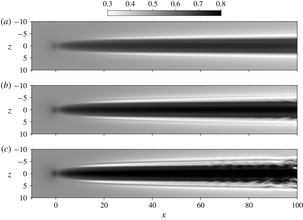
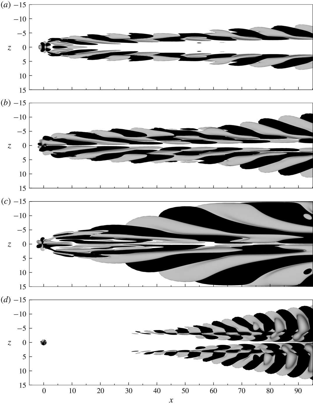
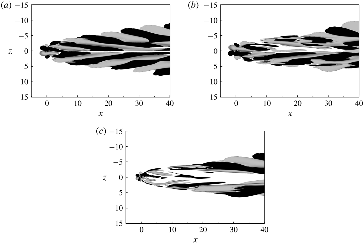
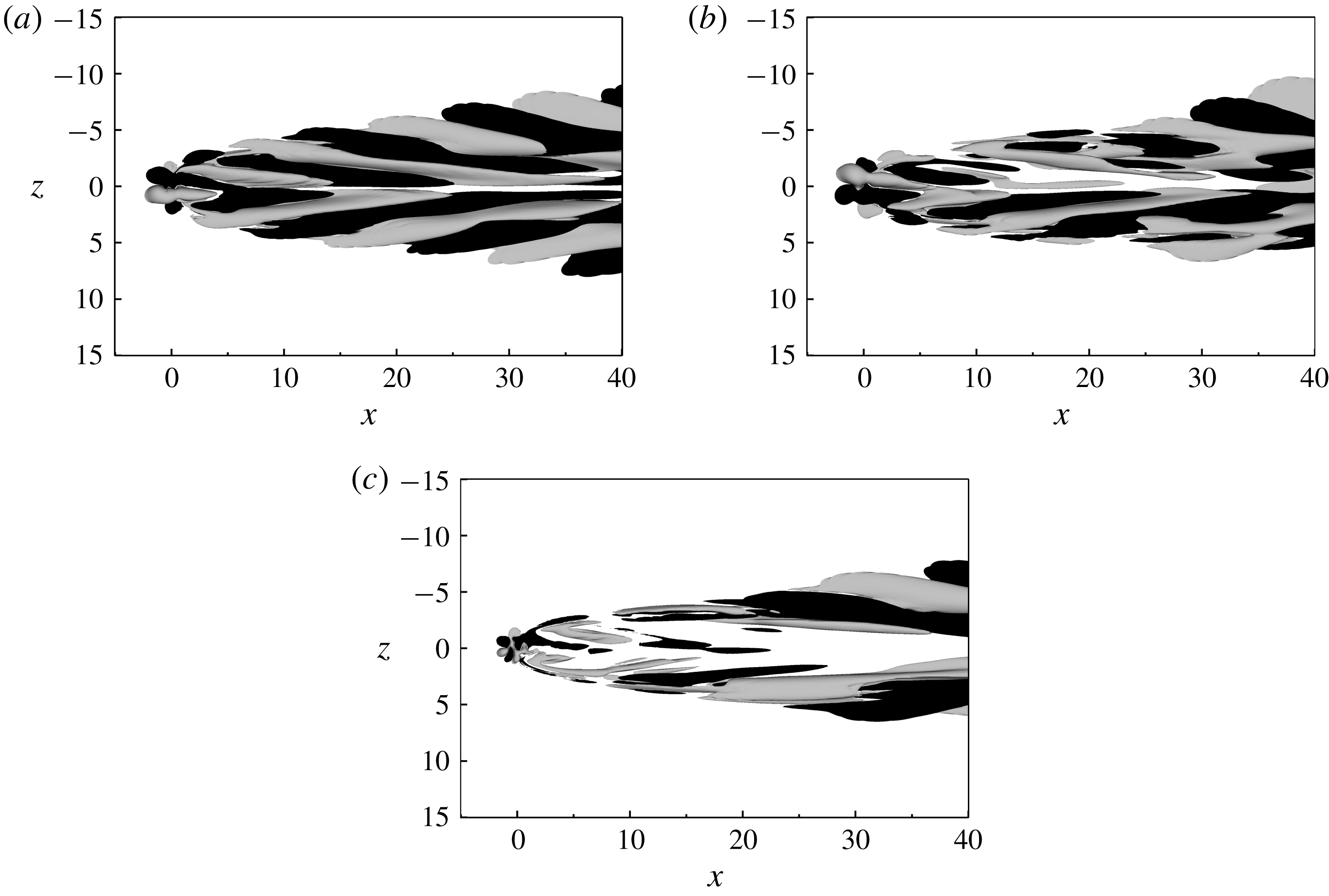
Flow visualisation of streamwise velocity for (a)
 $R=0.452$
, (b)
 $R=0.678$
and (c)
 $R=0.905$
, at
 $y=0.9$
(viewed from above).

In the thesis by Müller (Reference Müller2012), three cases were studied with the values
 $d^{\ast }/\unicode[STIX]{x1D6FF}_{h}^{\ast }=2$
,
 $Re_{\unicode[STIX]{x1D6FF}_{h}^{\ast }}=1924$
and
 $R=\{0.452,0.678,0.905\}$
(based on the same parameter definitions as in this work). These velocity ratios imply a pipe Reynolds number of
 $Re_{d}=\{1739.3,2608.9,3482.4\}$
(with
 $Re_{d}=|V_{h}^{\ast }|d^{\ast }/\unicode[STIX]{x1D708}^{\ast }$
). As a starting point for the present study, the three cases of Müller (Reference Müller2012) are reproduced. The simulations are started from the synthetic flow field
 $\boldsymbol{u}_{Bl-p}$
(see § 2.1) and integrated forward in time. The long-time flow responses are visualised in figure 3. For the lowest suction ratio shown in figure 3(a), an apparently stable boundary layer is obtained featuring a central high-speed streak and a counter-rotating vortex pair. With increased levels of suction, the strength of this streak increases, and as seen in figure 3(b), oscillations appear on the vortex legs towards the end of the domain. These oscillations are persistent in time, which is an indication that the flow might have surpassed its critical suction ratio
 $R_{crit}$
and become unstable. For even higher values of
 $R$
(figure 3
c), the vortices break down and turbulent flow develops in the wake. Based on these simulations, the critical suction ratio that precipitates boundary layer transition appears to be in the interval
 $0.452<R_{crit}<0.678$
(see figure 1 for a comparison with the aforementioned data available in the literature). The case with suction ratio
 $R=0.678$
is selected for further analysis. Before considering a spectral analysis of this configuration, some of its flow characteristics will be further highlighted.
3.2 Flow features
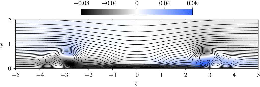
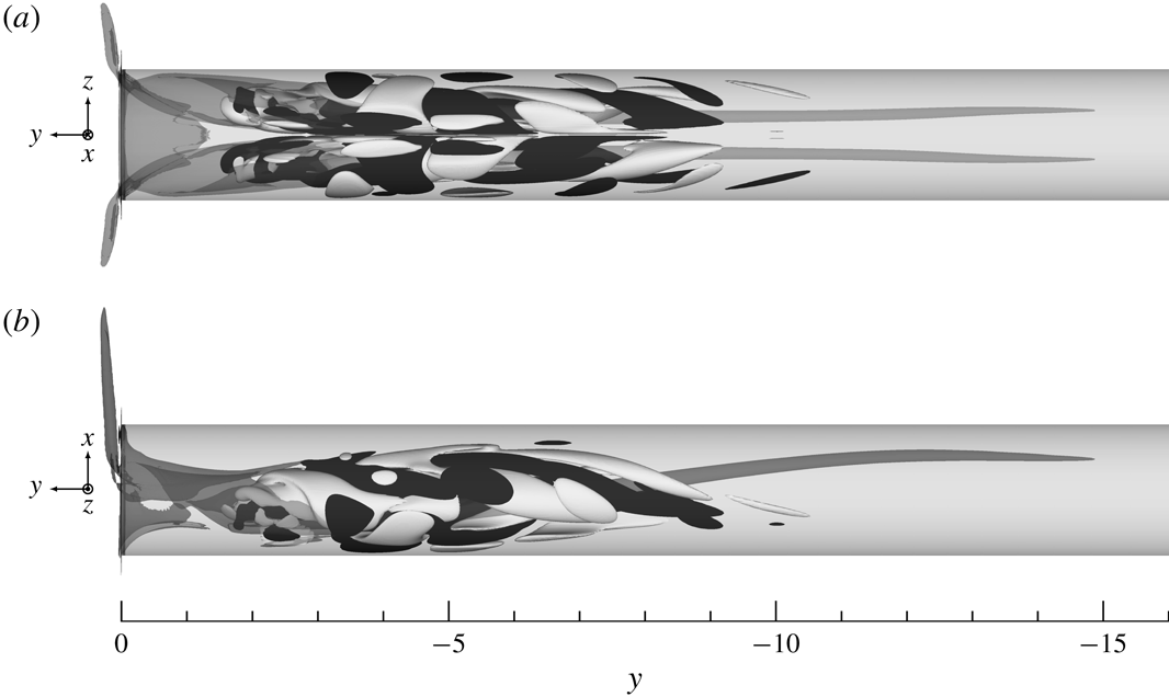
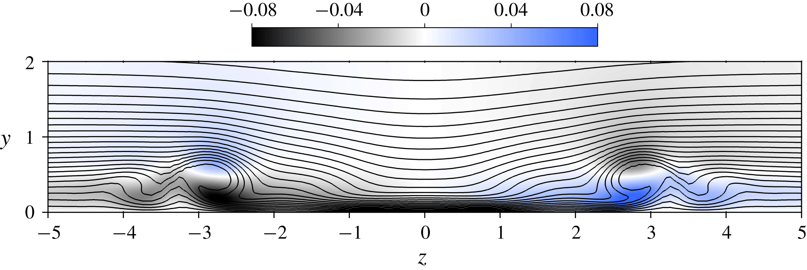
One of the most prominent structures in the flow is the counter-rotating vortex pair shown in figure 4. This pair of vortices originates inside the pipe and brings high-velocity fluid in the outer part of the boundary layer towards the plate, where it creates a high-speed streak behind the suction hole as shown in figure 5. Outside of the primary vortex pair, there is a weak secondary vortex pair with a sense of rotation that is opposite to the principal one, followed by a third slightly stronger vortex pair that co-rotates with the principal one. Similar vortex structures have also been reported by (Meyer Reference Meyer1955; MacManus & Eaton Reference MacManus and Eaton1998, Reference MacManus and Eaton2000). MacManus & Eaton (Reference MacManus and Eaton1998, Reference MacManus and Eaton2000) argued that these secondary vortices may arise due to the strongly inflectional spanwise velocity component (see figure 5).
Vortex structures for the suction ratio of
 $R=0.678$
visualised by the
 $\unicode[STIX]{x1D706}_{2}$
-criterion (Jeong & Hussain Reference Jeong and Hussain1995). The view is from above, and the sense of rotation of the different vortices are indicated by their colour and the arrows.

Velocity in the
 $yz$
-plane at
 $x=10$
(
 $x^{\ast }/d^{\ast }=5$
) for the suction ratio
 $R=0.678$
(viewed from upstream). Isocontours of the streamwise velocity component are shown with black lines (ranging from
 $0.0$
to
 $1.0$
and separated by
 $0.04$
units) and the spanwise velocity is shaded.
Visualisation of the instantaneous flow inside the pipe at various distance from the pipe inflow. The out-of-plane
 $y$
-velocity is shaded, and positive and negative
 $y$
-vorticity is shown with yellow and blue contours, respectively, and ranges from
 $-29.0$
to
 $29.0$
with
 $1$
unit separation.
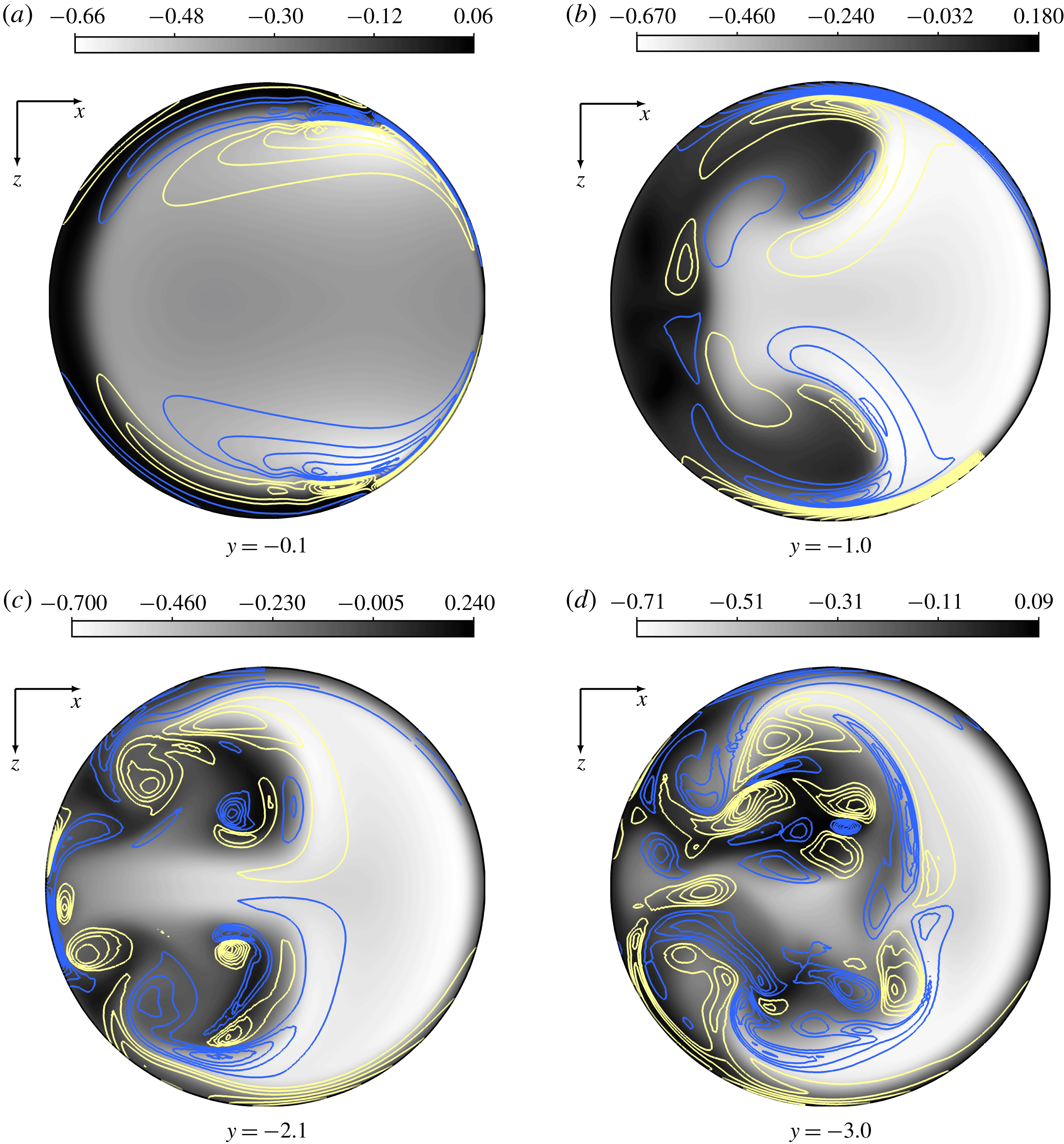
Regarding the flow within the pipe, a separated zone develops at the upstream side of the pipe wall close to the pipe junction, as plotted in figure 6. Further down in the pipe, the counter-rotating vortices create two streaks with fluid moving in the upward direction that are symmetrically positioned about the
 $xy$
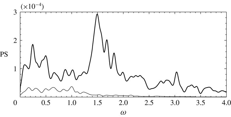
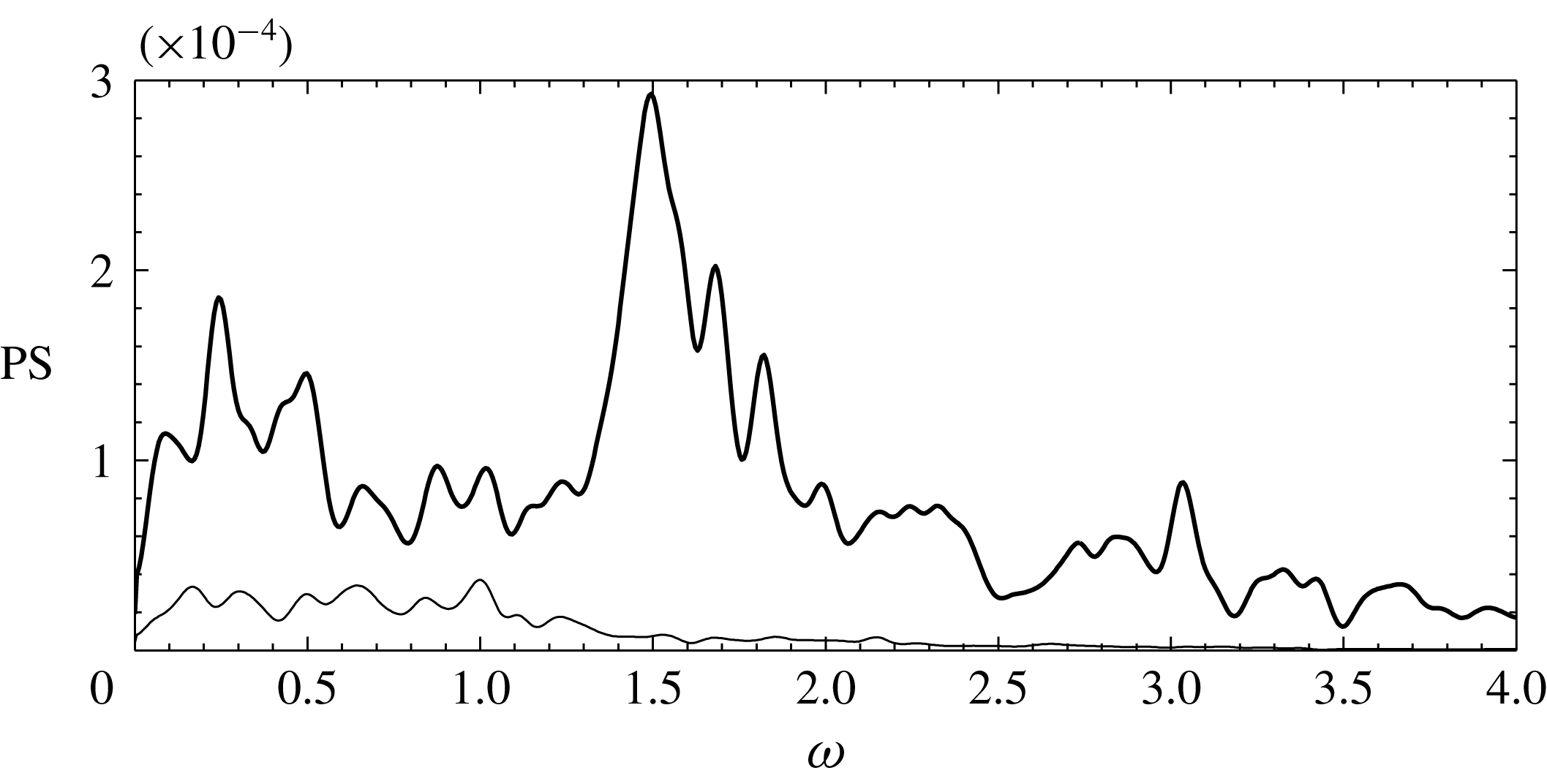
-plane. These streaks move away from the wall with distance from the inlet and grow into very intricate structures that eventually destabilise and trip the flow inside the pipe. This breakdown is further illustrated in figure 7 where typical power spectra (PS) from two probes within the pipe are shown. These power spectra are computed from the
 $x$
-velocity component using Welch’s method of averaged modified periodograms (see e.g. Heinzel, Rüdiger & Schilling Reference Heinzel, Rüdiger and Schilling2002), where each segment has been windowed with a Hann function using an overlap of 50 %. (The length of each segment was approximately 123 time units, and the effective noise bandwidth of the window was 0.0122.) Near the inlet of the pipe (
 $5\unicode[STIX]{x1D6FF}_{h}^{\ast }$
from the pipe inflow), large energetic structures appear with several amplified frequencies. Further down into the pipe (
 $20\unicode[STIX]{x1D6FF}_{h}^{\ast }$
from the pipe inflow), these large structures have broken down and consequently their corresponding energies have decreased.
Power spectra (PS) of the
 $x$
-velocity (cross-stream component) measured in the pipe at the positions
 $(0.0,-5.0,-0.5)$
(——) and
 $(0.0,-20.0,-0.5)$
(——).
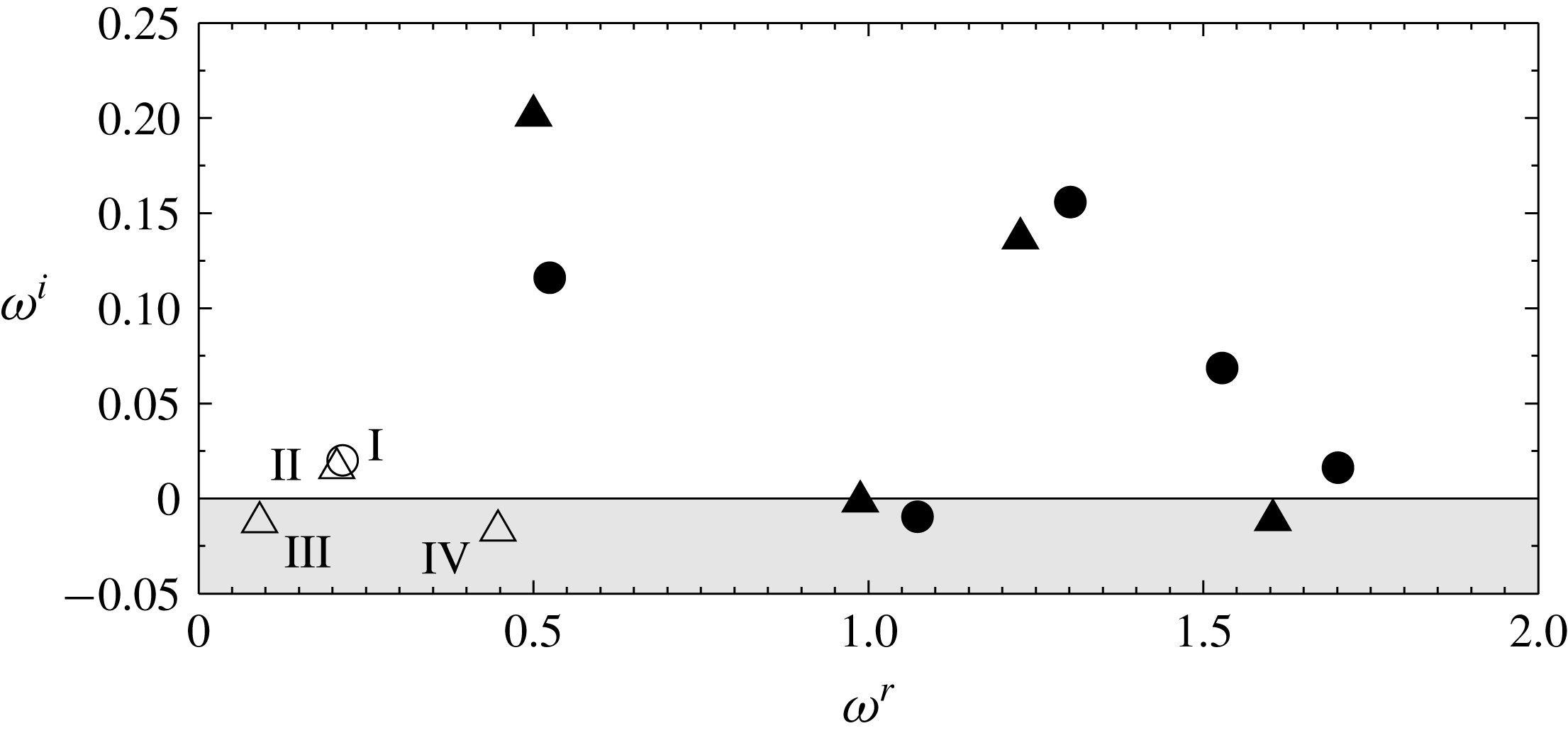
Eigenvalue spectrum for
 $R=0.678$
(the superscripts
 $r$
and
 $i$
refer to the real and the imaginary parts of
 $\unicode[STIX]{x1D714}$
, respectively). The eigenvalues whose corresponding eigenvectors have their support only in the pipe are marked with filled symbols, whereas eigenvalues whose eigenvectors have their support in the pipe and in the boundary layer are marked with open symbols. The eigenvectors have different symmetries and are either varicose (○) or sinuous (▵).
A separation bubble and a pair of counter-rotating vortices have also been observed in the simulations presented by MacManus & Eaton (Reference MacManus and Eaton1996). However, for their comparably low values of
 $R$
, no unsteadiness of the separation bubble was seen. The inhomogeneity of the vertical velocity component near the pipe inlet (figure 6
a) was also observed in the compressible simulations by Müller (Reference Müller2012) using flow parameters comparable to the present ones. However, in contrast to figures 6 and 7, that author did not report any unsteadiness inside the pipe, but rather argued for the opposite. The reason for this difference in results is unknown. In fact, a preliminary DNS study on a coarser grid investigating different parameter combinations of
 $R$
and
 $Re_{\unicode[STIX]{x1D6FF}_{h}^{\ast }}$
, suggests that for the present values of
 $d$
,
 $s$
and
 $L$
, the pipe always transitions for a lower
 $R$
or
 $Re_{\unicode[STIX]{x1D6FF}_{h}^{\ast }}$
than the boundary layer (Brynjell-Rahkola et al.
Reference Brynjell-Rahkola, Barman, Peplinski, Hanifi and Henningson2015). Consequently, the separation bubble and flow conditions in the pipe seem to play a crucial role in the transition process.
3.3 Linear stability analysis
The eigenvalue spectrum containing the most unstable/least stable eigenvalues for the case with the intermediate suction ratio
 $R=0.678$
are plotted in figure 8. (Since the spectrum is symmetric about the imaginary axis, only half of it is shown.) Comparison of these eigenvalues with the spectra plotted in figure 7 shows a quite good agreement between the linear analysis and the DNS. All of the eigenvectors have their support in the pipe and a few modes also extend into the boundary layer. As can be seen, many of the modes inside the pipe are highly unstable, whereas two modes in the boundary layer (and the pipe) are slightly unstable, and another two are lightly dampened. In contrast, a preliminary stability analysis (Brynjell-Rahkola et al.
Reference Brynjell-Rahkola, Barman, Peplinski, Hanifi and Henningson2015) performed on a coarser mesh suggests that all the modes for
 $R=0.452$
that contain both the boundary layer and the pipe are stable (in agreement with the nonlinear DNS results of § 3.1).
Two kinds of symmetry are observed among the eigenvectors. One where the
 $x$
- and
 $y$
-components are anti-symmetric and the
 $z$
-component is symmetric with respect to the
 $xy$
-plane, and another where this symmetry is reversed (i.e. the
 $x$
- and
 $y$
-components are symmetric and the
 $z$
-component is anti-symmetric). Throughout the rest of this article, modes with these different symmetries will be referred to as sinuous and varicose, respectively.
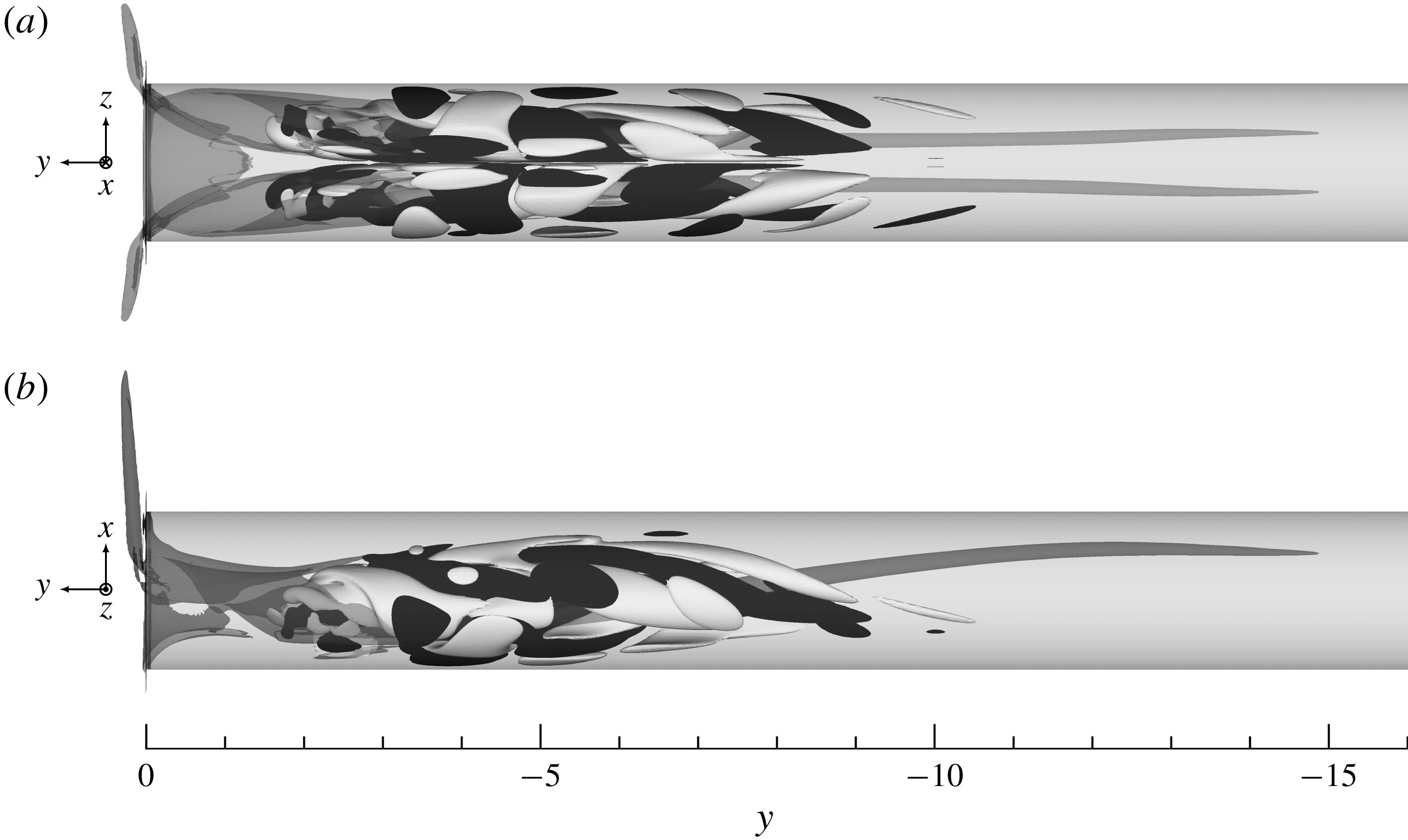
In figure 9, the most unstable eigenvector (a sinuous pipe mode) is shown. The mode resides close to the pipe inlet in the same region where the flow was seen to destabilise and break down in the DNS simulation (figure 6). In fact, the five most unstable (pipe) modes have their maximum amplitude in the interval
 $-6<y<-3$
. This shows that the transition to turbulence observed in the pipe section to a large extent can be explained by an instability near the pipe inlet. Instabilities that are restricted to the pipe would, however, not be able to explain the origin of oversuction since amplification of such modes does not imply disturbance growth within the boundary layer. This can be realised by considering the lower suction ratio
 $R=0.452$
, for which the pipe flow transitions to turbulence while the boundary layer remains laminar. Therefore, given the aim of understanding the origin of oversuction, the boundary layer modes will be studied in greater detail throughout the remainder of this article.
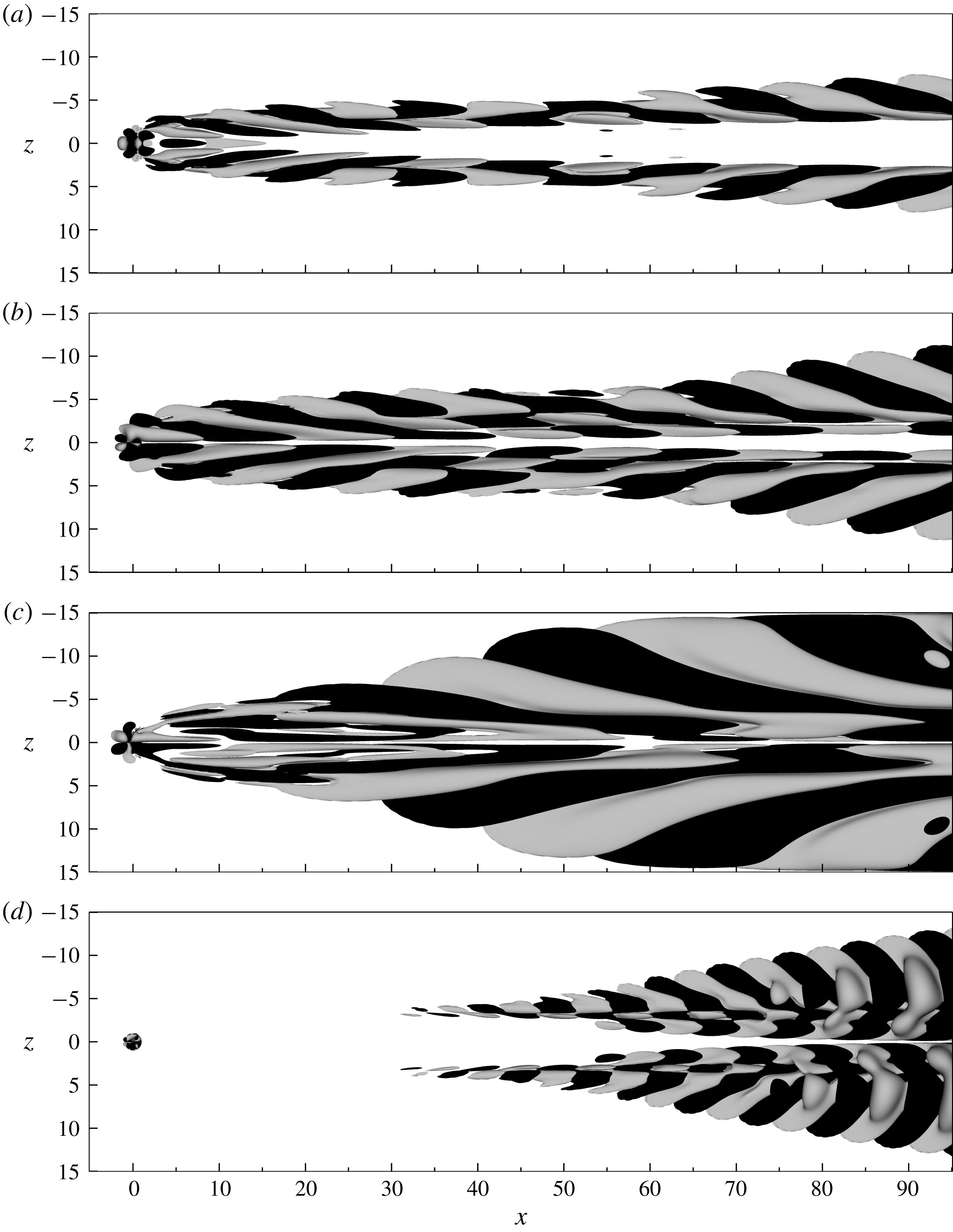
The eigenvalues whose eigenvectors span both the pipe and the boundary layer are labelled I–IV in figure 8. Their corresponding eigenvectors are shown in figure 10. Like the other modes, the modes I–IV are strongest in the pipe, but in contrast to the other ones, the eigenvectors also have a weak tail that extends into the boundary layer. Although the amplitudes of these eigenvectors are between
 $O(10^{-4})$
and
 $O(10^{-2})$
lower in the boundary layer than in the pipe, our analysis will show that it is precisely these motions that are responsible for the transition in the boundary layer.
As seen in figure 10, the unstable modes I and II have different symmetries. Since the growth rate (and the frequency) of these modes are similar to each other, they can be expected to have similar amplitudes in the flow. Therefore the transition process is unlikely to exhibit a particular symmetry, as also indicated in figure 3.
Vertical velocity component of the eigenvector corresponding to the most unstable eigenvalue
 $\unicode[STIX]{x1D714}=\pm 0.4997+\text{i}0.2014$
. Contours corresponding to
 $\pm 1\,\%$
of the maximum velocity are plotted in white and black colours, respectively, together with base flow vortex structures visualised by the
 $\unicode[STIX]{x1D706}_{2}$
-criterion (Jeong & Hussain Reference Jeong and Hussain1995) (dark grey).
Streamwise velocity component of the eigenvectors corresponding to the eigenvalues labelled (a) I, (b) II, (c) III and (d) IV in figure 8. Contours corresponding to
 $\pm 0.1\unicode[STIX]{x2030}$
of the maximum velocity are plotted in grey and black colours, respectively.
Relative contributions from the production mechanisms to the growth rate in (3.2) for the selected modes. The tuples
 $(j,k)$
denote the different terms
 $-E_{\unicode[STIX]{x1D6FA}}^{-1}\int _{\unicode[STIX]{x1D6FA}}(\hat{u} _{j}^{r}\hat{u} _{k}^{r}+\hat{u} _{j}^{i}\hat{u} _{k}^{i})\unicode[STIX]{x2202}U_{j}/\unicode[STIX]{x2202}x_{k}\,\text{d}\unicode[STIX]{x1D6FA}$
normalised by
 $|\unicode[STIX]{x1D714}^{i}|$
. The numbering in the first column refers to the mode labelling introduced in figure 8.

Relative contributions from the dissipation mechanisms to the growth rate in (3.2) for the selected modes. The tuples
 $(j,k)$
denote the different terms
 $E_{\unicode[STIX]{x1D6FA}}^{-1}Re_{\unicode[STIX]{x1D6FF}_{h}^{\ast }}^{-1}\int _{\unicode[STIX]{x1D6FA}}[(\unicode[STIX]{x2202}\hat{u} _{j}^{r}/\unicode[STIX]{x2202}x_{k})^{2}+(\unicode[STIX]{x2202}\hat{u} _{j}^{i}/\unicode[STIX]{x2202}x_{k})^{2}]\,\text{d}\unicode[STIX]{x1D6FA}$
normalised by
 $|\unicode[STIX]{x1D714}^{i}|$
. The numbering in the first column refers to the mode labelling introduced in figure 8.

Valuable information regarding the mechanisms promoting the growth of these modes can be obtained by considering the temporal evolution of the perturbation energy
 $E_{\unicode[STIX]{x1D6FA}}$
as described by the Reynolds–Orr equation. This equation is derived from (2.5) (see Schmid & Henningson Reference Schmid and Henningson2001) and reads
 $$\begin{eqnarray}\frac{\text{d}E_{\unicode[STIX]{x1D6FA}}}{\text{d}t}=-\int _{\unicode[STIX]{x1D6FA}}u_{j}^{\prime }u_{k}^{\prime }\frac{\unicode[STIX]{x2202}U_{j}}{\unicode[STIX]{x2202}x_{k}}\,\text{d}\unicode[STIX]{x1D6FA}-\frac{1}{Re_{\unicode[STIX]{x1D6FF}_{h}^{\ast }}}\int _{\unicode[STIX]{x1D6FA}}\frac{\unicode[STIX]{x2202}u_{j}^{\prime }}{\unicode[STIX]{x2202}x_{k}}\frac{\unicode[STIX]{x2202}u_{j}^{\prime }}{\unicode[STIX]{x2202}x_{k}}\,\text{d}\unicode[STIX]{x1D6FA}-\int _{\unicode[STIX]{x1D6FA}}\unicode[STIX]{x1D6FE}u_{j}^{\prime }u_{j}^{\prime }\,\text{d}\unicode[STIX]{x1D6FA},\end{eqnarray}$$
wherein two similar indices imply summation, and
 $j,k\in \{1,2,3\}$
. Indices
 $\{1,2,3\}$
hence refer to the three spatial directions
 $\{x,y,z\}$
, respectively. The first term on the right-hand side of (3.1) represents the exchange of energy between the perturbation and the base flow (i.e. energy production), the second term represents dissipation of energy by viscosity and the third term corresponds to a volume force (here taken to be the sponge force that makes the disturbance vanish on the inflow and outflow boundaries). By substituting the mode ansatz of § 2.2.2 into (3.1), an equation for the growth rate of a mode may be derived
 $$\begin{eqnarray}\displaystyle \unicode[STIX]{x1D714}^{i} & = & \displaystyle -\frac{1}{E_{\unicode[STIX]{x1D6FA}}}\int _{\unicode[STIX]{x1D6FA}}(\hat{u} _{j}^{r}\hat{u} _{k}^{r}+\hat{u} _{j}^{i}\hat{u} _{k}^{i})\frac{\unicode[STIX]{x2202}U_{j}}{\unicode[STIX]{x2202}x_{k}}\,\text{d}\unicode[STIX]{x1D6FA}-\frac{1}{E_{\unicode[STIX]{x1D6FA}}}\frac{1}{Re_{\unicode[STIX]{x1D6FF}_{h}^{\ast }}}\int _{\unicode[STIX]{x1D6FA}}\left[\left(\frac{\unicode[STIX]{x2202}\hat{u} _{j}^{r}}{\unicode[STIX]{x2202}x_{k}}\right)^{2}+\left(\frac{\unicode[STIX]{x2202}\hat{u} _{j}^{i}}{\unicode[STIX]{x2202}x_{k}}\right)^{2}\right]\,\text{d}\unicode[STIX]{x1D6FA}\nonumber\\ \displaystyle & & \displaystyle -\,\frac{1}{E_{\unicode[STIX]{x1D6FA}}}\int _{\unicode[STIX]{x1D6FA}}\unicode[STIX]{x1D6FE}[(\hat{u} _{j}^{r})^{2}+(\hat{u} _{j}^{i})^{2}]\,\text{d}\unicode[STIX]{x1D6FA},\end{eqnarray}$$
from which the contributions of the different production and dissipation terms to the growth or decay of a given eigenmode can be evaluated. The superscripts
 $r$
and
 $i$
refer to the real and imaginary parts, respectively, and the energy of the perturbation in the domain is given by
 $E_{\unicode[STIX]{x1D6FA}}=\int _{\unicode[STIX]{x1D6FA}}(\hat{u} _{j}^{r2}+\hat{u} _{j}^{i2})\,\text{d}\unicode[STIX]{x1D6FA}$
. (In the stability computations the eigenvectors are normalised to have
 $E_{\unicode[STIX]{x1D6FA}}=1$
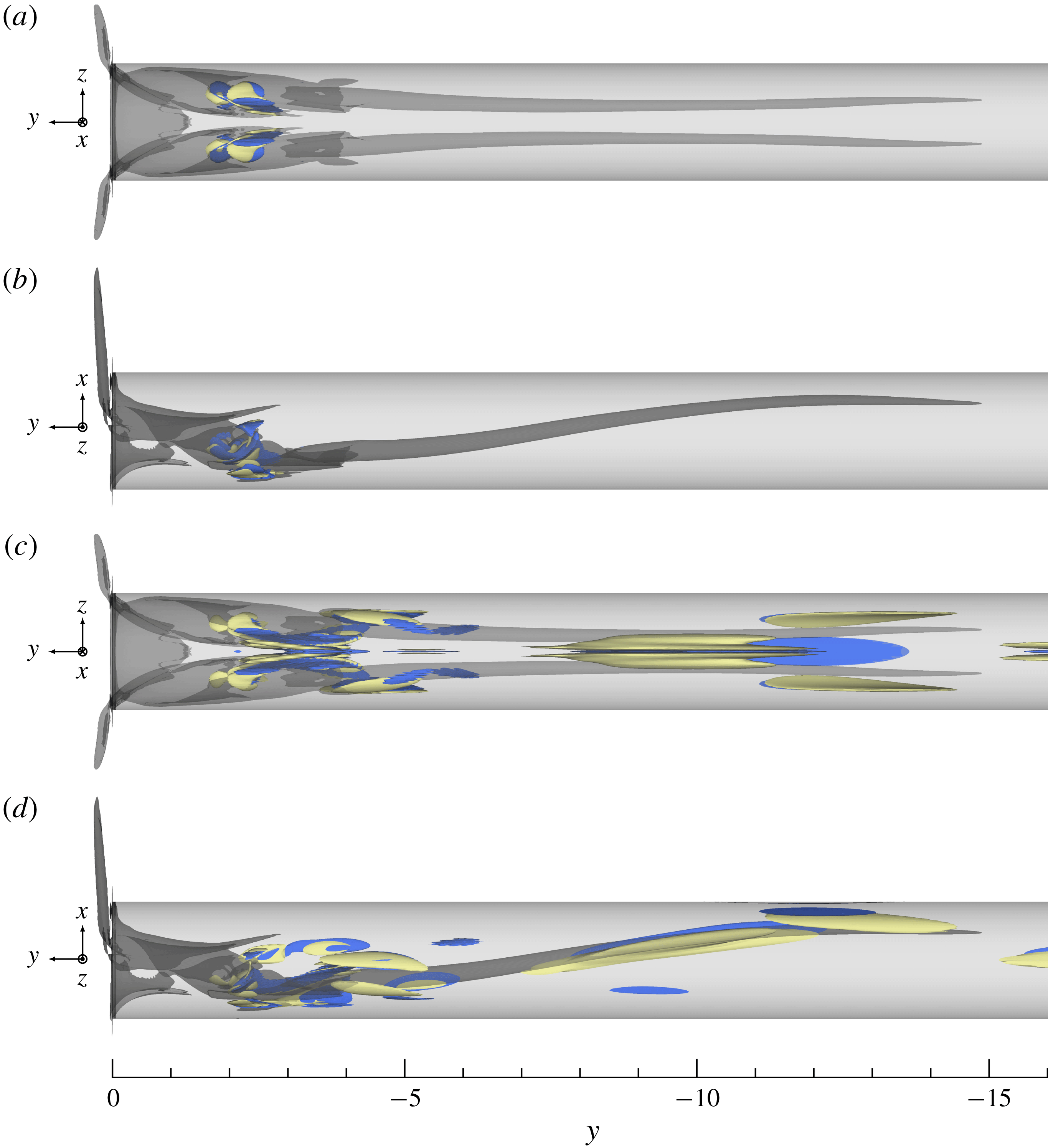
.) The results of evaluating the terms in (3.2) are given in tables 2 and 3, which state the individual production and dissipation mechanisms, respectively.
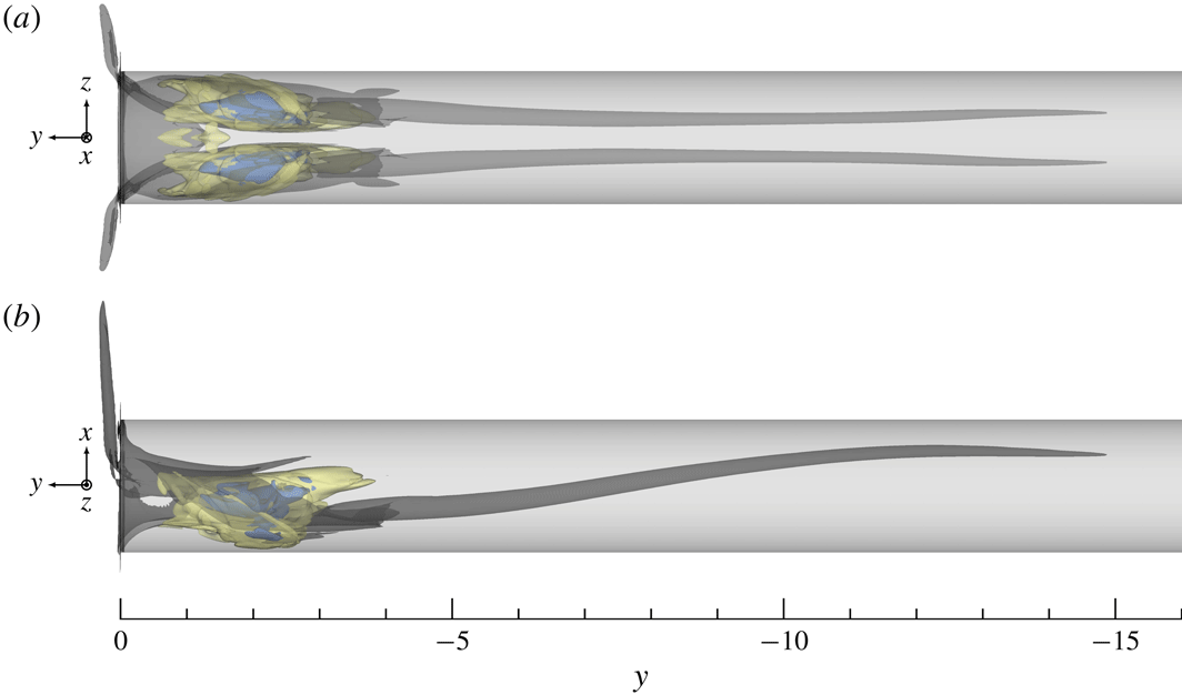
Density of the sum of all production (yellow) and dissipation (blue) mechanisms for (a,b) mode I and (c,d) mode II. Contours corresponding to 10 % of the maximum production/dissipation of kinetic energy are plotted together with base flow vortex structures visualised by the
 $\unicode[STIX]{x1D706}_{2}$
-criterion (Jeong & Hussain Reference Jeong and Hussain1995) (dark grey).
By examining table 2, it is noted that the production of energy generally is dominated by either
 $-E_{\unicode[STIX]{x1D6FA}}^{-1}\int _{\unicode[STIX]{x1D6FA}}(\hat{v}^{r}\hat{u} ^{r}+\hat{v}^{i}\hat{u} ^{i})\unicode[STIX]{x2202}V/\unicode[STIX]{x2202}x\,\text{d}\unicode[STIX]{x1D6FA}$
or
 $-E_{\unicode[STIX]{x1D6FA}}^{-1}\int _{\unicode[STIX]{x1D6FA}}(\hat{v}^{r}{\hat{w}}^{r}+\hat{v}^{i}{\hat{w}}^{i})\unicode[STIX]{x2202}V/\unicode[STIX]{x2202}z\,\text{d}\unicode[STIX]{x1D6FA}$
. For mode I and IV it is the former whereas for II and III it is the latter. This implies that energy is extracted from the base flow and transferred to the eigenmodes by vertical and horizontal components of the eigenvectors working against the gradients of the vertical base flow component in the horizontal directions. Similarly, by studying table 3, it is observed that the main mechanisms responsible for dissipation of energy are the horizontal gradients of the vertical eigenvector component, i.e.
 $E_{\unicode[STIX]{x1D6FA}}^{-1}Re_{\unicode[STIX]{x1D6FF}_{h}^{\ast }}^{-1}\int _{\unicode[STIX]{x1D6FA}}[(\unicode[STIX]{x2202}\hat{v}^{r}/\unicode[STIX]{x2202}x)^{2}+(\unicode[STIX]{x2202}\hat{v}^{i}/\unicode[STIX]{x2202}x)^{2}]\,\text{d}\unicode[STIX]{x1D6FA}$
for modes I and IV, and
 $E_{\unicode[STIX]{x1D6FA}}^{-1}Re_{\unicode[STIX]{x1D6FF}_{h}^{\ast }}^{-1}\int _{\unicode[STIX]{x1D6FA}}[(\unicode[STIX]{x2202}\hat{v}^{r}/\unicode[STIX]{x2202}z)^{2}+(\unicode[STIX]{x2202}\hat{v}^{i}/\unicode[STIX]{x2202}z)^{2}]\,\text{d}\unicode[STIX]{x1D6FA}$
for modes II and III.
In figure 11 the density functions of the sum of all production and dissipation mechanisms for modes I and mode II are visualised. As seen, the plotted structures are symmetric with respect to the
 $xy$
-plane and have a rather different shape for the two eigenmodes. For the varicose mode I, the production and dissipation of kinetic energy are localised close to the pipe inlet beneath the separation bubble that forms on the upstream portion of the wall. For the sinuous mode II on the other hand, production and dissipation of kinetic energy seem to be associated with both the aforementioned region close to the pipe inlet, and the elongated vortex legs that extend through the pipe.
Since the instability of the eigenmodes I and II is modest, small changes in the numerical set-up may have a large impact on the overall character of the boundary layer. In order to ensure that these modes are converged in terms of resolution, the polynomial order is increased from
 $N=12$
to
 $N=15$
(mesh M2). This change doubles the number of grid points, but changes the absolute value of the eigenvalues for the two modes by less than 1 %. (The changes in the absolute value of the eigenvalues corresponding to the pipe modes are
 $O(0.1\,\%)$
.)
Figure 10 shows that all the encountered modes in the boundary layer extend towards the end of the domain where they are dampened by the sponge function. Recent three-dimensional stability analyses considering the flow around a cylindrical roughness element in a Blasius boundary layer have shown that eigenmodes corresponding to isolated eigenvalues can be rather insensitive to changes in the domain size, given that sufficiently long domains are considered (Loiseau et al.
Reference Loiseau, Robinet, Cherubini and Leriche2014). In contrast, eigenvalues corresponding to the flow around a cylindrical roughness element in a Falkner–Skan–Cooke boundary layer have been shown to be impossible to converge with respect to the domain size (Brynjell-Rahkola et al.
Reference Brynjell-Rahkola, Shahriari, Schlatter, Hanifi and Henningson2017) due to the presence of acceleration and sweep. In order to verify the sensitivity of this parameter on the present flow case, the streamwise extent of the boundary layer is increased by approximately 25 % (mesh M3). However, this changes the eigenvalues of mode I and II less than
 $0.1\unicode[STIX]{x2030}$
in absolute value, which suggests that the instability mechanisms of the boundary layer are independent of the box length and localised in the domain. (The changes in the absolute value of the eigenvalues corresponding to the pipe modes are
 $O(0.01\unicode[STIX]{x2030})$
.)
3.4 Sensitivity
Next, the origin of the instability reported in § 3.3 is investigated. This is done through a structural sensitivity analysis as introduced by Giannetti & Luchini (Reference Giannetti and Luchini2007). These authors considered a spatially localised perturbation to the linearised Navier–Stokes equations (2.5) in the form of a force–velocity coupling, and they derived an upper bound for the resulting eigenvalue drift due to this perturbation. Following their analysis, regions in space where the flow is sensitive and where a localised force feedback thus will create a large change in a given eigenvalue, may be identified by evaluating the expression
 $$\begin{eqnarray}\unicode[STIX]{x1D707}(\boldsymbol{x})=\Vert \hat{\boldsymbol{u}}^{\dagger }(\boldsymbol{x})\Vert \Vert \hat{\boldsymbol{u}}(\boldsymbol{x})\Vert ,\end{eqnarray}$$
for a pair of direct and adjoint eigenvectors subject to the normalisation
 $$\begin{eqnarray}\max _{\boldsymbol{x}\in \unicode[STIX]{x1D6FA}}\{|\hat{u} (\boldsymbol{x})|\}=1,\quad \int _{\unicode[STIX]{x1D6FA}}|\hat{\boldsymbol{u}}^{\dagger }\boldsymbol{\cdot }\hat{\boldsymbol{u}}|\,\text{d}\unicode[STIX]{x1D6FA}=1,\end{eqnarray}$$
(
 $\Vert \cdot \Vert$
is the Euclidean norm in
 $\mathbb{C}^{3}$
). As argued by Chomaz (Reference Chomaz2005) and Giannetti & Luchini (Reference Giannetti and Luchini2007), regions where
 $\unicode[STIX]{x1D707}(\boldsymbol{x})$
is non-zero may be ascribed the role of a ‘wavemaker’ that indicates where in space the instability mechanism resides. Equation (3.3) and (3.4) evaluated for mode I is visualised in figure 12. As seen, the ‘wavemaker’-region is localised inside the pipe beneath the separation bubble. It is symmetric about the
 $xy$
-plane and embraces the vertical elongated vortices that form in the pipe and were seen to break down in figure 6. Comparing the isocontours corresponding to 1 % and 10 % of the maximum value, it is noted that the sensitivity increases towards the centre of the pipe. This implies that the ‘core’ of the instability lies on the inner sides of the two vortices, and thus that a small control device will have the largest impact on the instability if placed between the two vortex legs. The corresponding region for mode II has a similar shape, strength and location.
Structural sensitivity. Contours of
 $\unicode[STIX]{x1D707}$
corresponding to 10 % (blue) and 1 % (yellow) of the maximum sensitivity for mode I are plotted together with base flow vortex structures visualised by the
 $\unicode[STIX]{x1D706}_{2}$
-criterion (Jeong & Hussain Reference Jeong and Hussain1995) (dark grey).

Sensitivity to momentum forcing. Contours corresponding to 5 % (yellow), 15 % (blue) and 50 % (black) of the maximum value of (a)
 $\Vert \hat{\boldsymbol{u}}_{III}^{\dagger }\Vert$
and (b)
 $\Vert \hat{\boldsymbol{u}}_{IV}^{\dagger }\Vert$
are plotted (
 $\Vert \cdot \Vert$
is the Euclidean norm in
 $\mathbb{C}^{3}$
).

Since mode III and mode IV are asymptotically stable, they will ultimately decay in time unless they are excited by a harmonic driving force. It is therefore of interest to also consider the sensitivity of these modes to forcing. As described by Hill (Reference Hill1995), the sensitivity of a given flow to momentum sources may be assessed by studying the adjoint eigenvectors. The adjoint eigenvectors exhibit the same symmetry as their corresponding direct eigenvectors. In figure 13 the norm of the adjoint eigenvectors corresponding to modes III and IV (here denoted
 $\hat{\boldsymbol{u}}_{III}^{\dagger }$
and
 $\hat{\boldsymbol{u}}_{IV}^{\dagger }$
, respectively) are visualised. By comparing the spatial distribution of the sensitivity of the two modes, it is seen that both are susceptible to momentum disturbances that enter through the sucked streamtube. However, the low frequency mode appears more sensitive to lateral forcing, whereas the high frequency mode is more sensitive to forcing directly in front of the hole. In addition to the boundary layer, the adjoint eigenvectors are also seen to reach into the pipe and cover the pipe junction and the separation bubble. Due to the presence of the unstable modes, excitation of the lightly dampened modes III and IV can thus be expected to appear through momentum forcing by the unsteady fluctuations in the pipe and around the pipe orifice. As a result, these modes, although asymptotically stable, are likely to be excited and contribute to the transition process in the boundary layer.
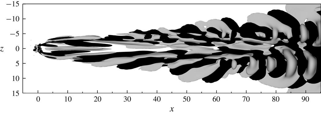
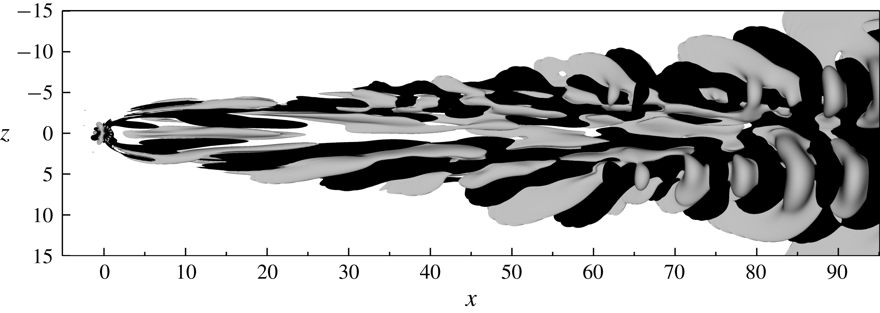
An instantaneous snapshot of the unsteady disturbance component of a nonlinear DNS. Contours of the streamwise velocity component
 $u-U$
corresponding to
 $\pm 10^{-4}$
are plotted in grey and black colours, respectively.
3.5 Analysis of the nonlinear flow
With this insight into the stability and receptivity of the flow, it is instructive to study how well the results from the linear analysis apply to the nonlinear flow, and to what extent they can be used to interpret the transition scenario observed. To obtain a first qualitative picture of the disturbance field present in the DNS, the steady base flow solution is subtracted from the instantaneous velocity field shown in figure 3(b). The resulting unsteady component of the flow is plotted in figure 14. This shows the presence of an unsteady perturbation with spatially varying wavelength in the aft of the suction hole that is reminiscent of the modes shown in figure 10. Note that the velocity in the DNS and the base flow is
 $O(1)$
, and thus that the strength of the perturbation in the boundary layer is comparable to the relative strength of the eigenvectors in the boundary layer.
A brief comparison of the frequency content in the DNS and in the linear analysis was presented in figures 7 and 8. However, in order to make any strong conclusions regarding the transition of the boundary layer flow, it is important to verify that the disturbance in the boundary layer has the characteristics of the linear eigenmodes I–IV. To this end, a Koopman analysis as described in § 2.3 is carried out. Given the large amplitude ratio of the disturbance between the pipe and the boundary layer, this analysis will be limited to a smaller subset of the domain, namely
 $[-25,40]\times [0,15]\times [-15,15]$
. This choice will prevent the strong fluctuations in the pipe as well as in the downstream portions of the plate from contaminating and overshadowing the relevant linear mechanisms that initiate the transition process in the boundary layer. Around 300 snapshots are sampled consecutively in time from the nonlinear DNS with a separation of
 $\unicode[STIX]{x0394}\tilde{t}=0.48$
. (The columns of
 $\unicode[STIX]{x1D730}_{0}^{m}$
span an approximate subspace with a residual whose Euclidean norm is below
 $10^{-5}$
.) The time integration is started from the flow field visualised in figure 3(b), which corresponds to an arbitrary time instance after transients have washed away.
The spectral content of the flow in the specified subdomain is plotted in figure 15. As seen, the flow features several amplified frequencies. Among the frequencies, the three most amplified ones are seen to be (in order)
 $\tilde{\unicode[STIX]{x1D714}}=0.2258$
,
 $0.1112$
and
 $0.1933$
, which are in reasonable agreement with the frequencies of the modes I, III and II that were obtained in the linear analysis, i.e.
 $\unicode[STIX]{x1D714}^{r}=0.2155$
,
 $0.0913$
and
 $0.2062$
, respectively.
Frequency spectrum of the Koopman operator (the mean flow is omitted). The amplitudes
 $|D_{k}|$
of the different frequencies are computed from (2.17) and normalised by that of the mean flow,
 $|D_{1}|$
.

In figure 16, the shape of the Koopman modes corresponding to these frequencies are visualised. In figures 16(a) and 16(b), the modes corresponding to the frequencies
 $\tilde{\unicode[STIX]{x1D714}}=0.1933$
and
 $\tilde{\unicode[STIX]{x1D714}}=0.2258$
are shown, respectively. As seen, the former closely resemble the sinuous mode visualised in figure 10(b). The latter on the other hand appears quite noisy and is somewhat difficult to interpret. It appears to be a combination of a sinuous and a varicose mode. Since the modes I and II from the linear analysis have similar frequencies and growth rates, it is possible that the DMD algorithm is unable to fully distinguish between the two, which might explain its distorted structure. In figure 16(c) the mode corresponding to frequency
 $\tilde{\unicode[STIX]{x1D714}}=0.1112$
is shown. The shape of this mode is again in good agreement with the sinuous mode III visualised in figure 10(c). The Koopman analysis is also able to identify the frequency
 $\tilde{\unicode[STIX]{x1D714}}=0.4464$
, which is very close to that of the linear mode IV with
 $\unicode[STIX]{x1D714}^{r}=0.4469$
. However, as seen in figure 10(d), this mode is relatively weak in the subdomain considered here (
 $-25\leqslant x\leqslant 40$
) and can therefore not be expected to appear as a peak in the current analysis.
Streamwise velocity component of the Koopman modes corresponding to the frequencies (a)
 $\tilde{\unicode[STIX]{x1D714}}=0.1933$
, (b)
 $\tilde{\unicode[STIX]{x1D714}}=0.2258$
and (c)
 $\tilde{\unicode[STIX]{x1D714}}=0.1112$
. Contours corresponding to
 $\pm 1\,\%$
of the maximum velocity are plotted in grey and black colours, respectively.
4 Discussion and conclusions
In this article, the classical problem of oversuction in a flat plate boundary layer has been revisited and novel insight into its origin has been presented. The study focuses on a single infinite row of widely spaced circular suction pipes that act in isolation. For the cases investigated, unsteady fluctuations and transition are always observed within the pipe. However, upon increasing the suction ratio while keeping other parameters fixed, unsteadiness also develops in the boundary layer. A linear stability analysis shows that these fluctuations correspond to two unstable eigenmodes that reside in the pipe and extend into the boundary layer. Among the unstable modes, two symmetries with respect to the
 $xy$
-plane are distinguished, namely varicose and sinuous. This implies that the transition in the boundary layer generally can be expected to be asymmetric.
The computed eigenvalues appear to be rather insensitive to small changes in the numerics such as resolution and domain size. This means that the instability can be regarded as a robust phenomenon, which enables an upper limit on the suction ratio to be defined (for a given Reynolds number and hole geometry) at which the boundary layer will be tripped. In the present study, the sensitivity of the flow with respect to the pipe length
 $L^{\ast }/d^{\ast }$
has not been explicitly investigated. However, as seen in figure 12, the region of structural sensitivity for mode I is limited to
 $y>-5$
, while the total length of the pipe is
 $L=40$
. This suggests that a modification in the computational set-up far away from the pipe junction will have a minor effect on the corresponding eigenvalue (Giannetti & Luchini Reference Giannetti and Luchini2007). A similar analysis performed on the other modes reported in figure 8 leads to the same conclusion, which suggests that changes in the pipe length will have a negligible influence on the dynamics of the flow.
In the study by MacManus & Eaton (Reference MacManus and Eaton1996), the impact of the geometry of the suction hole on the vorticity generated behind the orifice was numerically investigated. They concluded that the specific shape of the hole (i.e. bore type, rounded inlet, asymmetrically rounded inlet and rounded raised lip) had little influence on the level of induced vorticity, and that the largest change was obtained by inclining the holes. In contrast to these findings, the structural sensitivity presented herein suggests that the pipe inlet and the associated separation bubble are the regions where the flow is most sensitive to modifications in the geometry and boundary conditions. In fact, one may infer from these findings that a proper lip shaping may significantly shift the eigenvalues, and hence possibly increase the critical suction parameters of the flow.
Over the years, several explanations have been proposed for the origin of oversuction (see § 1). In this work, it is for the first time shown that, although transition becomes visible in the boundary layer far downstream of the suction orifice, the instability is actually initiated in the pipe section around the elongated vortex pair and the separation bubble. From an energy budget, the dominating mechanisms that produce and dissipate kinetic energy are determined. It is shown that the unstable varicose mode mainly gains energy from the
 $x$
- and
 $y$
-components of the perturbation working against the base flow gradient
 $\unicode[STIX]{x2202}V/\unicode[STIX]{x2202}x$
, whereas the unstable sinuous mode mainly gains energy from the
 $y$
- and
 $z$
-components of the perturbation working against the base flow gradient
 $\unicode[STIX]{x2202}V/\unicode[STIX]{x2202}z$
. By increasing the amount of suction, the size of the recirculation zone near the pipe inlet will decrease, while the strength of the vortex pair will increase. This suggests that the base flow gradients in these regions will become sharper, and by increasing the suction levels beyond a given threshold, a critical level of shear in the
 $x$
- and
 $z$
-directions is surpassed, which triggers the instability. An examination of the density functions for the sum of the production terms reveals that the varicose mode primarily extracts energy from the region close to the inlet and the separation bubble. The sinuous mode on the other hand is found to be able to extract energy from a larger region in space involving not only the aforementioned region, but also the region between and around the vortex legs further down into the pipe. This is an indication that the varicose mode (for the present flow parameters) can be interpreted as an instability of the separation bubble, and that the sinuous mode can be interpreted as an instability of both the separation bubble and the vortex legs.
An interesting question is how these unstable modes compare to those obtained from a stability analysis about a time-averaged mean flow. Such a comparison was for instance performed by Barkley (Reference Barkley2006) for the two-dimensional flow around a cylinder. Barkley showed that beyond the bifurcation point, the frequency of an unstable mode deduced from a mean flow analysis closely matched that of a limit cycle oscillation, whereas the frequency obtained from a base flow analysis did not. This observation was further analysed by Sipp & Lebedev (Reference Sipp and Lebedev2007), who considered a multiple time-scale analysis of the flow near critical conditions and described the amplitude of the first unstable mode by a Stuart–Landau equation. These authors showed that the mean flow analysis does not always predict the frequency of a nonlinear limit cycle correctly, and proposed necessary conditions for such an analysis to be meaningful. As an alternative approach, the spectral properties of a nonlinear flow can be analysed using Koopman analysis (Mezić Reference Mezić2013). Such an analysis has been performed in the present study, and the resulting Koopman eigenvalues and Koopman modes are found to agree well with the eigenvalues and the eigenvectors of the linearised operator around the base flow. Furthermore, the eigenvalue spectrum obtained from the base flow analysis is found to compare quite well with the frequency spectrum obtained from a velocity probe in the pipe of the nonlinear DNS. Such agreement may seem surprising given that the flow inside the pipe transitions, and the vortex structures from which the unstable boundary layer modes extract energy thus break down. However, as shown in figure 12, the ‘cores’ of the instability mechanisms are localised close to the pipe inlet where the oscillations typically are small (see figure 6). Hence, the structures of the mean flow and the base flow in this dynamically important region are likely to be similar, which explains the observed agreement. This establishes the presence of the computed modes in the transition process, and corroborates that the premature transition observed in many experiments indeed can be explained by a linear instability of the flow.
Acknowledgements
We wish to thank E. Barman for performing a preliminary study that served as a starting point for this work. We thank Dr A. Peplinski for help with mesh generation and for providing the tools used in the linear stability analysis. P. S. Negi is acknowledged for a good collaboration on the implementation of the DMD algorithm, and Professor P. Schlatter is acknowledged for discussions. The simulations have been performed at the PDC Center for High Performance Computing and the National Supercomputer Centre (NSC) in Sweden with computer time granted by the Swedish National Infrastructure for Computing (SNIC).