1. Introduction
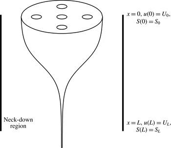
Microstructured optical fibres (or MOFs) are thin strands of glass, distinguished from solid optical fibres by the cross-sectional structure running along their length. The design of this cross-sectional structure, which acts to change the refractive index from that of the pure glass, gives the fibre certain optical and physical properties that are desirable in a range of applications (see, for instance, Monro & Ebendorff-Heidepriem Reference Monro and Ebendorff-Heidepriem2006). In the context of this work we focus on fibres with internal air channels. These fibres typically have diameters of hundreds of micrometres, with the internal channels being of even smaller diameter (typically of the order of the wavelength of light). These fibres are manufactured by slowly feeding a preform of suitable geometry (typically 1–3 cm in diameter) into a heated region within a furnace and then stretching the molten glass to the dimensions of a fibre. A diagram of this process is shown in figure 1, where the preform is fed into the furnace with feed speed
 $U_{0}$
and the stretched fibre is drawn off with speed
 $U_{L}$
by winding the fibre onto a spool at some distance away from the neck-down region over which the stretching occurs. This neck-down region is comparable in length, but not necessarily identical, to the heated region of the furnace.
The process of drawing a preform into a fibre may significantly deform the internal geometry, so that the resulting cross-section of the fibre is not simply a rescaled version of the preform. Rather it will be modified under the influence of effects such as surface tension and channel pressurisation so that the relative position and shape of the channels is altered from the preform to the fibre. In modelling this process and the associated deformation of the geometric configuration there are two broad objectives: firstly, given a known preform, to determine the shape of the resulting fibre (the forward problem); secondly, to determine the preform design and draw parameters that are required to produce a desired fibre geometry (the inverse problem).
It is possible to control the change in internal geometry by carefully selecting the operational draw parameters (such as draw speed
 $U_{L}$
and furnace temperature). An extra degree of control, one that will be the focus of this work, may be obtained by the active pressurisation of channels. Here, the internal channels are held at a higher pressure than the ambient environment. This acts to expand channels in the cross-sectional geometry, opposing surface tension which tends to shrink these small-scale structures as the fibre is drawn. While it is known that the cross-sectional geometry is very sensitive to the pressure, recent experimental work by Kostecki et al. (Reference Kostecki, Ebendorff-Heidepriem, Warren-Smith and Monro2014) has shown that it is feasible to use active pressurisation to achieve fine control of the geometry. Such pressurisation is necessary, for instance, in designs that feature internal channels of very small diameter, which are pressurised so that they are not closed completely by surface tension. Pressure is also applied to expand a preform geometry, an example being a fibre that features narrow walls between the channels (see the experimental work of Kostecki et al. (Reference Kostecki, Ebendorff-Heidepriem, Warren-Smith and Monro2014) for examples). Such a design would be difficult to achieve without pressurisation since it is problematic to manufacture a preform with very thin walls.
Schematic diagram of the neck-down region.

A number of previous studies have investigated the effect of active pressurisation, including Fitt et al. (Reference Fitt, Furusawa, Monro, Please and Richardson2002) who modelled a fibre with an annular cross-section and Chen & Birks (Reference Chen and Birks2013) who recognised the importance of fibre tension in determining channel deformation in this fundamental case. Fitt et al. (Reference Fitt, Furusawa, Monro, Please and Richardson2002) found a closed-form solution for this simple geometry where channel pressurisation was considered in the absence of surface tension. They also derived a closed-form solution where both effects were included under the assumption that the inner channel diameter was small compared to the outer diameter of the fibre, but did not draw any conclusions about the competition between the two effects without this restriction. The case of an annular fibre will be reconsidered in detail in the present work without any such restriction on the relative size of the inner channel.
Channel pressurisation may be introduced in more subtle ways. Self-pressurisation, for instance, is introduced if there is a difference between the enclosed volume of air entering at the top of the neck-down region and the volume drawn off in the fibre, so that the deformation of the internal geometry can effectively induce extra pressurisation. Although the mechanism behind this effect, as considered in detail by Voyce et al. (Reference Voyce, Fitt, Hayes and Monro2009) for preforms that are sealed at both ends, will not be considered here, there is a natural overlap between active and self-pressurisation and the model presented here might be used, in conjunction with experimental results, to determine the magnitude of self-pressurisation.
In modelling the fibre drawing process a Lagrangian framework will be adopted. Earlier authors have made use of Eulerian approaches in modelling fibre drawing, in particular Yarin, Gospodinov & Roussinov (Reference Yarin, Gospodinov and Roussinov1994) and Fitt et al. (Reference Fitt, Furusawa, Monro, Please and Richardson2002), and this approach is suited to examining certain aspects of these problems. Lagrangian coordinate systems, exploiting the slenderness of the geometry, have also been used to model extensional flows more generally (Wilson Reference Wilson1988; Yarin Reference Yarin1993; Stokes, Tuck & Schwartz Reference Stokes, Tuck and Schwartz2000; Wylie, Huang & Miura Reference Wylie, Huang and Miura2011). In particular, Dewynne, Howell & Wilmott (Reference Dewynne, Howell and Wilmott1994) introduced a Lagrangian approach to model the stretching of solid fibres and showed that the three-dimensional fibre drawing problem may be written in terms of a one-dimensional extensional flow in the direction of the fibre axis and a two-dimensional Stokes-flow free-boundary problem in the cross-plane perpendicular to this axis. A limitation of that work was the neglect of surface tension. Cummings & Howell (Reference Cummings and Howell1999) built on this approach by including surface tension. An important feature of their work was the scaling of the cross-plane problem with the square root of its area and the introduction of a Lagrangian ‘reduced time’ variable that reduced it to a classical Stokes-flow free-boundary problem in a domain of unit area with unit surface tension. This problem gives the deformation of the cross-section due to surface tension. The extensional and cross-plane models are coupled, but crucially the cross-plane flow may be solved completely independently of the axial flow. The approach of Cummings & Howell (Reference Cummings and Howell1999) was used by Griffiths & Howell (Reference Griffiths and Howell2007, Reference Griffiths and Howell2008) to study the stretching of thin-walled viscous tubes and they derived elegant asymptotic solutions of these problems.
The modelling approach used in the present work will build on recent work by some of the current authors (Stokes et al. Reference Stokes, Buchak, Crowdy and Ebendorff-Heidepriem2014; Buchak et al. Reference Buchak, Crowdy, Stokes and Ebendorff-Heidepriem2015), who demonstrated the utility of this approach for fibres of arbitrary cross-plane geometry. The key feature of their model, which led to this result, was writing the extensional flow model in terms of the reduced time variable rather than the Eulerian spatial coordinate. This very general approach is a particularly important advance for modelling the drawing of MOFs, which feature very complicated cross-sectional geometries that have many internal interfaces. Note that the model of Griffiths & Howell (Reference Griffiths and Howell2007, Reference Griffiths and Howell2008) is, in fact, a specific example of the underlying mathematical structure of the more general fibre drawing problem as detailed in full by Stokes et al. (Reference Stokes, Buchak, Crowdy and Ebendorff-Heidepriem2014).
The key result of Stokes et al. (Reference Stokes, Buchak, Crowdy and Ebendorff-Heidepriem2014) is to show that it is possible to explicitly describe the solution to the axial stretching problem in terms of the cross-sectional geometry. For any cross-sectional geometry this solution can be expressed in terms of a single function
 $$\begin{eqnarray}H({\it\tau})=\exp \left(-\frac{1}{12}\int _{0}^{{\it\tau}}\tilde{{\it\Gamma}}({\it\tau}^{\prime })\,\text{d}{\it\tau}^{\prime }\right),\end{eqnarray}$$
where
 ${\it\tau}$
is the Lagrangian reduced time coordinate and
 $\tilde{{\it\Gamma}}$
is the total circumference of all cross-sectional boundaries scaled with the square root of cross-sectional area, which is calculated from the solution to the cross-plane problem. Once this intermediate quantity
 $H({\it\tau})$
has been determined, all other axial quantities may be described in terms of it, namely the cross-sectional area
 $S$
, the axial velocity
 $u$
and the axial coordinate
 $x$
. For the isothermal case (with constant viscosity), these quantities are
 $$\begin{eqnarray}\displaystyle & \displaystyle S({\it\tau})=\frac{1}{H({\it\tau})^{2}}\left(1-\frac{{\it\sigma}^{\ast }}{{\it\gamma}^{\ast }}\int _{0}^{{\it\tau}}H({\it\tau}^{\prime })\,\text{d}{\it\tau}^{\prime }\right)^{2}, & \displaystyle\end{eqnarray}$$
 $$\begin{eqnarray}\displaystyle & \displaystyle u({\it\tau})=\frac{1}{S({\it\tau})}, & \displaystyle\end{eqnarray}$$
 $$\begin{eqnarray}\displaystyle & \displaystyle x({\it\tau})=-\frac{1}{{\it\sigma}^{\ast }}\log \left(H({\it\tau})\sqrt{S({\it\tau})}\right). & \displaystyle\end{eqnarray}$$
 ${\it\gamma}^{\ast }$
is a scaled surface tension parameter,
 ${\it\sigma}^{\ast }$
is a scaled fibre tension parameter and the ratio between these two parameters is proportional to the dimensional fibre tension. Knowledge of this dimensional quantity is of great practical use in fibre drawing since it allows an experimentalist to predict from the model the change in internal geometry due to the tension in the fibre, which is an easily measurable quantity in an experimental setting.
In Buchak et al. (Reference Buchak, Crowdy, Stokes and Ebendorff-Heidepriem2015) this model is used for MOFs having complex cross-plane geometries with many elliptical internal air channels, by using a generalisation of the elliptical pore model of Crowdy (Reference Crowdy2004) to solve the cross-plane problem. This provides a fast and accurate reduction of the full free-boundary problem to a coupled system of nonlinear ordinary differential equations and, more significantly, regularises the ill-posed inverse problem of determining the initial preform geometry and draw parameters to draw a MOF with a desired cross-plane geometry.
The current work will extend that of Stokes et al. (Reference Stokes, Buchak, Crowdy and Ebendorff-Heidepriem2014) and Buchak et al. (Reference Buchak, Crowdy, Stokes and Ebendorff-Heidepriem2015) by including channel pressurisation. As will be seen, the inclusion of this effect changes the mathematical structure of the model since it is no longer possible to solve the cross-plane problem independently of the axial flow. As a consequence, the approach outlined above involving
 $H({\it\tau})$
is not valid, since the two sub-models for the axial and cross-plane flows are now fully coupled and must be solved simultaneously. Details of the extended model with channel pressurisation included are given in § 2.
In § 3 the model is applied to the case of a fibre with an annular cross-section. Our Lagrangian approach reveals several new details of this fundamental case with pressurisation, without the restrictions of previous studies such as Fitt et al. (Reference Fitt, Furusawa, Monro, Please and Richardson2002), who made several assumptions about the magnitude of various physical parameters which we do not. In particular, our model gives a criterion for fibre explosion on application of sufficiently large pressure (that is, the boundary of the inner channel expands to the point where it meets the outer boundary), namely
 $$\begin{eqnarray}p_{H}>\frac{4}{3}\frac{1}{S_{0}}\sqrt{\frac{1-{\it\rho}_{0}}{1+{\it\rho}_{0}}}\left({\it\sigma}\sqrt{\frac{1-{\it\rho}_{0}}{1+{\it\rho}_{0}}}+2\sqrt{{\rm\pi}}{\it\gamma}\sqrt{S_{0}}\right),\end{eqnarray}$$
where
 ${\it\rho}_{0}$
is the aspect ratio of the preform,
 $S_{0}$
is the cross-sectional glass area of the preform,
 $p_{H}$
is the pressure applied to the channel,
 ${\it\sigma}$
is the fibre tension and
 ${\it\gamma}$
is the surface tension.
Several cases for fibres with multiple pressurised channels are considered in § 4. It is assumed that the cross-sectional shapes of the channels are ellipses and the cross-plane problem with pressurised channels is solved, as described in Buchak et al. (Reference Buchak, Crowdy, Stokes and Ebendorff-Heidepriem2015), using the generalised elliptical pore model. One example will be of particular interest to experimentalists, where we consider an inverse problem to optimally design a preform for a multi-hole fibre such that the preform design features (nearly) circular channels. This is an important practical consideration when preforms are to be fabricated by drilling holes in a billet of glass (where drilled holes are, by nature, circular) or by stacking capillaries with circular inner channels.
Our results are summarised and conclusions given in § 5.
2. Formulation
A schematic diagram of the fibre drawing process is given in figure 1. This shows the ‘neck-down’ region over which the preform is stretched to the dimensions of a fibre. As indicated in the diagram, the modelling approach adopted here will allow for multiple channels running down the length of the fibre, and these channels may be held at a pressure different to the ambient environment.
As in figure 1, the axial coordinate
 $x$
is directed along the axis of the fibre in the direction of the stretching, with the coordinates
 $y$
and
 $z$
in the cross-sectional plane perpendicular to this axis. The velocities in these directions are
 $u$
,
 $v$
and
 $w$
, respectively, and
 $p$
is pressure in the fluid (as opposed to the pressure in the channels). The cross-sectional area of the fibre varies in the axial direction and this area is denoted by
 $S(x)$
, while the total length of all boundaries in a cross-section at position
 $x$
is denoted by
 ${\it\Gamma}(x)$
. The modelling region is from
 $x=0$
to
 $x=L$
, where
 $L$
is the ‘neck-down’ length. Several boundary conditions are imposed on the flow, namely that
 $u=U_{0}$
,
 $S=S_{0}$
at
 $x=0$
and
 $u=U_{L}$
at
 $x=L$
. Where, as in the inverse problem, the desired structure of the final fibre, rather than that of the preform, is known, the area at the end of the draw
 $S=S_{L}$
at
 $x=L$
is imposed instead of the condition on the area at
 $x=0$
. A key parameter is the draw ratio, defined as
 $$\begin{eqnarray}D=\frac{U_{L}}{U_{0}},\end{eqnarray}$$
and it is typically the case that
 $D>1$
for fibre drawing. There are
 $N$
internal channels and so it is necessary to consider
 $N+1$
free boundaries (including the outer boundary). The cross-sectional areas enclosed by each boundary are denoted as
 $\mathscr{A}^{(k)}$
for
 $k=0\ldots N$
, where
 $\mathscr{A}^{(0)}$
is the area enclosed by the outer boundary, which includes the internal holes, and
 $\mathscr{A}^{(k)}$
is the area of the
 $k$
th channel. Similarly, the pressure in the ambient environment is
 $p^{(0)}$
and the applied pressure in the
 $k$
th channel is
 $p^{(k)}$
for
 $k=1\ldots N$
.
Following Dewynne, Ockendon & Wilmott (Reference Dewynne, Ockendon and Wilmott1992), Cummings & Howell (Reference Cummings and Howell1999), Griffiths & Howell (Reference Griffiths and Howell2008) and Stokes et al. (Reference Stokes, Buchak, Crowdy and Ebendorff-Heidepriem2014), it is assumed that the fibre geometry is slender (that is
 $\sqrt{S}\ll L$
). This assumption allowed those authors to introduce a slenderness parameter
 ${\it\epsilon}=\sqrt{S_{0}}/L$
and obtain a leading-order approximation to the Navier–Stokes equations consisting of two coupled models for the flow in the axial and cross-plane directions. The same approach is adopted here. The spatial coordinates, time, velocities, pressure and other variables are scaled as
 $$\begin{eqnarray}\displaystyle & \displaystyle (x,y,z)=L(x^{\ast },{\it\epsilon}y^{\ast },{\it\epsilon}z^{\ast }), & \displaystyle\end{eqnarray}$$
 $$\begin{eqnarray}\displaystyle & \displaystyle t=\frac{L}{U_{0}}t^{\ast }, & \displaystyle\end{eqnarray}$$
 $$\begin{eqnarray}\displaystyle & \displaystyle (u,v,w)=U_{0}(u^{\ast },{\it\epsilon}v^{\ast },{\it\epsilon}w^{\ast }), & \displaystyle\end{eqnarray}$$
 $$\begin{eqnarray}\displaystyle & \displaystyle p=\frac{{\it\mu}_{0}U_{0}}{L}p^{\ast }, & \displaystyle\end{eqnarray}$$
 $$\begin{eqnarray}\displaystyle & \displaystyle S=S_{0}S^{\ast }, & \displaystyle\end{eqnarray}$$
 $$\begin{eqnarray}\displaystyle & \displaystyle {\it\Gamma}={\it\epsilon}L{\it\Gamma}^{\ast }, & \displaystyle\end{eqnarray}$$
 ${\it\gamma}$
and fluid viscosity
 ${\it\mu}$
, are scaled thus:
 $$\begin{eqnarray}\displaystyle & \displaystyle {\it\gamma}=\frac{{\it\mu}_{0}U_{0}\sqrt{S_{0}}}{L}{\it\gamma}^{\ast }, & \displaystyle\end{eqnarray}$$
 $$\begin{eqnarray}\displaystyle & \displaystyle {\it\mu}(x)={\it\mu}_{0}{\it\mu}^{\ast }(x), & \displaystyle\end{eqnarray}$$
 ${\it\mu}_{0}$
is a typical value for viscosity in the flow. In the examples considered in §§ 3 and 4 it will be assumed that
 ${\it\mu}^{\ast }(x)=1$
. As seen in work by Taroni et al. (Reference Taroni, Breward, Cummings and Griffiths2013), for instance, the axial variation of viscosity may be modelled with a great deal of sophistication by accounting for conduction in the glass, but this is not the focus of the present study. As in Stokes et al. (Reference Stokes, Buchak, Crowdy and Ebendorff-Heidepriem2014) the final fibre geometry may be determined from the measured fibre tension and does not depend on a specific viscosity profile over the neck-down length but, rather, the harmonic mean of the viscosity over this length. Thus, without loss of generality so far as determining the geometry of the final fibre is concerned, we may set
 ${\it\mu}^{\ast }(x)=1$
so that
 ${\it\mu}_{0}$
is the harmonic mean of
 ${\it\mu}(x),0\leqslant x\leqslant L$
.
The axial and cross-plane models, resulting from the above scalings, are restated below with the effect of channel pressurisation included. As will be seen in §§ 2.1 and 2.2 below, the axial model is unchanged (at least in the case where the additional pressure is assumed, as it will be throughout this paper, to be independent of axial position), while there is an additional term in the stress condition on each boundary in the cross-plane model due to the internal pressure (see equation (2.2) in Buchak et al. Reference Buchak, Crowdy, Stokes and Ebendorff-Heidepriem2015).
2.1. Leading-order axial model
The derivation of the equations governing the axial flow for fibres with unpressurised channels is given in detail by Stokes et al. (Reference Stokes, Buchak, Crowdy and Ebendorff-Heidepriem2014). Since the derivation of this model is essentially the same for pressurised channels this will not be repeated in full here with the key additional steps outlined below and some further detail given in appendix A.
The assumption of slender geometry allows a leading-order approximation in the slenderness parameter
 ${\it\epsilon}^{2}$
to the full Navier–Stokes equations. The leading-order equations for conservation of mass and conservation of axial momentum, for small Reynolds number, are
 $$\begin{eqnarray}\displaystyle & \displaystyle Su=1, & \displaystyle\end{eqnarray}$$
 $$\begin{eqnarray}\displaystyle & \displaystyle (3{\it\mu}^{\ast }Su_{x})_{x}+\frac{1}{2}{\it\gamma}^{\ast }{\it\Gamma}_{x}-p_{x}^{\ast (0)}\mathscr{A}^{(0)}+\mathop{\sum }_{k=1}^{N}p_{x}^{\ast (k)}\mathscr{A}^{(k)}=0, & \displaystyle\end{eqnarray}$$
 ${\it\mu}^{\ast }$
,
 ${\it\gamma}^{\ast }$
and
 $p^{\ast (k)}$
. In the present work we only consider channels held at a fixed (constant) pressure. Although axially varying pressurisations are not considered here, they may be of interest in modelling self-pressurisation effects, as described by Voyce et al. (Reference Voyce, Fitt, Hayes and Monro2009), for instance. Since the pressurisations are constant, the two last terms in (2.11) vanish, and after integration over
 $x$
the equation for axial momentum becomes
 $$\begin{eqnarray}-3{\it\mu}^{\ast }\frac{\text{D}S}{\text{D}t}+\frac{{\it\gamma}^{\ast }}{2}{\it\Gamma}=6{\it\sigma}^{\ast },\end{eqnarray}$$
where
 ${\it\sigma}^{\ast }$
is a dimensionless parameter relating to fibre tension. By convention the dimensional tension in the fibre is
 ${\it\sigma}$
and these two quantities are related via
 $$\begin{eqnarray}{\it\sigma}=\frac{6{\it\mu}_{0}U_{0}S_{0}}{L}{\it\sigma}^{\ast }.\end{eqnarray}$$
Even though the problem is steady it is convenient to write (2.12) with a derivative following the motion since a Lagrangian coordinate system will later be introduced. Both (2.10) and (2.12) are identical to those obtained with no channel pressurisation; see Stokes et al. (Reference Stokes, Buchak, Crowdy and Ebendorff-Heidepriem2014).
A Lagrangian coordinate system is introduced, identical to that used in Cummings & Howell (Reference Cummings and Howell1999), Griffiths & Howell (Reference Griffiths and Howell2008) and Stokes et al. (Reference Stokes, Buchak, Crowdy and Ebendorff-Heidepriem2014). The time coordinate is
 $t=\tilde{t}$
and the axial coordinate is transformed via
 $$\begin{eqnarray}x=\int _{0}^{\tilde{t}}u(\tilde{x},T)\,\text{d}T+\tilde{x},\end{eqnarray}$$
where
 $\tilde{x}$
is the usual Lagrangian coordinate following the axial motion. The cross-plane lengths
 $y$
and
 $z$
are scaled with the square root of cross-sectional area
 ${\it\chi}=\sqrt{S(x,t)}$
so that these, as well as the total circumference
 ${\it\Gamma}$
, are transformed with
 $$\begin{eqnarray}y={\it\chi}{\tilde{y}},\quad z={\it\chi}\tilde{z},\quad {\it\Gamma}={\it\chi}\tilde{{\it\Gamma}}.\end{eqnarray}$$
As in Cummings & Howell (Reference Cummings and Howell1999), Griffiths & Howell (Reference Griffiths and Howell2008) and Stokes et al. (Reference Stokes, Buchak, Crowdy and Ebendorff-Heidepriem2014) a reduced time
 ${\it\tau}$
is introduced; this is defined by
 $$\begin{eqnarray}{\it\tau}={\it\gamma}^{\ast }\int _{0}^{\tilde{t}}\frac{\text{d}\tilde{t}}{{\it\mu}^{\ast }{\it\chi}}.\end{eqnarray}$$
The value of the reduced time at the end of the draw,
 ${\it\tau}(x=1)={\it\tau}_{L}$
, may be thought of as the total deformation time of the draw. In Stokes et al. (Reference Stokes, Buchak, Crowdy and Ebendorff-Heidepriem2014) this deformation time was shown to be simply proportional to the change in initial and final geometries, where this change was only due to surface tension. With channel pressurisation included the interpretation of
 ${\it\tau}_{L}$
is a little more subtle, since it will also take into account the action of this pressurisation against surface tension. This will be discussed in more detail in § 3.2.
Equations (2.10) and (2.12) may now be rewritten in terms of the Lagrangian reduced time coordinate
 ${\it\tau}$
to give
 $$\begin{eqnarray}\displaystyle & \displaystyle {\it\chi}^{2}({\it\tau})u({\it\tau})=1, & \displaystyle\end{eqnarray}$$
 $$\begin{eqnarray}\displaystyle & \displaystyle \frac{\text{d}{\it\chi}}{\text{d}{\it\tau}}-\frac{{\it\chi}}{12}\tilde{{\it\Gamma}}({\it\tau})=-\frac{{\it\sigma}^{\ast }}{{\it\gamma}^{\ast }}, & \displaystyle\end{eqnarray}$$
 $\tilde{{\it\Gamma}}({\it\tau})$
). In turn the solution to the whole problem was then described in terms of this integrating factor. This is not possible here since, unlike the case of fibre drawing without hole pressurisation and as was mentioned in the introduction and will be seen in § 2.2 below, the axial quantity
 ${\it\chi}$
now appears explicitly in the model for the cross-plane flow, meaning that the two models are fully coupled and this integrating factor approach, which relies on evaluating
 $\tilde{{\it\Gamma}}({\it\tau})$
independently of the axial flow, is no longer appropriate.
Finally, an expression for the physical coordinate
 $x$
is derived from the definition of reduced time (2.16), namely
 $$\begin{eqnarray}\frac{\text{d}x}{\text{d}{\it\tau}}=\frac{{\it\mu}^{\ast }(x)}{{\it\gamma}^{\ast }{\it\chi}}.\end{eqnarray}$$
This conversion back to the physical coordinate
 $x$
completes the axial model. Note that this last equation (2.19) is the only place in the axial model that features the viscosity
 ${\it\mu}^{\ast }(x)$
. Hence, the role of the axially varying viscosity
 ${\it\mu}^{\ast }(x)$
is to position a solution at a particular
 ${\it\tau}$
at a point in
 $x$
. Since the primary goal of this modelling is to investigate how the geometry of the final fibre differs from that of the initial preform, the precise detail of how this change occurs over the neck-down region is a subsidiary concern. As demonstrated in Stokes et al. (Reference Stokes, Buchak, Crowdy and Ebendorff-Heidepriem2014), the geometry change between the preform and the fibre is related to the harmonic mean of the viscosity profile. This may be seen by rearranging (2.19) and integrating to give an expression for the modelling parameter
 ${\it\gamma}^{\ast }$
, namely
 $$\begin{eqnarray}{\it\gamma}^{\ast }=\left.\int _{0}^{{\it\tau}_{L}}\frac{1}{{\it\chi}}\,\text{d}{\it\tau}\right/\!\!\int _{0}^{1}\frac{1}{{\it\mu}^{\ast }(x)}\,\text{d}x,\end{eqnarray}$$
where we have used the fact that
 $x({\it\tau}_{L})=1$
from the definition of reduced time. The integrals on the right-hand side of the above expression are the inverse harmonic means of the square root of cross-sectional area
 ${\it\chi}({\it\tau})$
and viscosity
 ${\it\mu}^{\ast }(x)$
, respectively. Thus, it is this integrated form of viscosity, rather than the full
 ${\it\mu}^{\ast }(x)$
profile in the neck-down region, that is required to determine the difference in the geometry between the preform and fibre. In practice, as established by Stokes et al. (Reference Stokes, Buchak, Crowdy and Ebendorff-Heidepriem2014) (and in a more restricted form by Chen & Birks (Reference Chen and Birks2013)), knowledge of the fibre tension
 ${\it\sigma}$
circumvents the need to know about viscosity. This is an important practical advance since, when actually performing a fibre draw, it is possible to measure fibre tension directly, but knowledge of the viscosity can only be imperfectly inferred from the furnace temperature. Put a different way, the fibre tension may be thought of as a measure of the integral viscosity or temperature over the neck-down region, which cannot be measured directly during fibre drawing.
2.2. Leading-order cross-plane model
The inclusion of channel pressurisation leads to a slightly altered version of the cross-plane model as compared to the unpressurised version of Stokes et al. (Reference Stokes, Buchak, Crowdy and Ebendorff-Heidepriem2014), with an extra term appearing in the leading-order stress conditions on the interfaces of the pressurised channels. In the notation here we allow for
 $N$
internal channels and have a pair of interfacial stress conditions for each channel, namely
 $$\begin{eqnarray}\displaystyle & \displaystyle (-p+2{\it\mu}^{\ast }v_{y})G_{y}^{(k)}+{\it\mu}^{\ast }(v_{z}+w_{y})G_{z}^{(k)}=-({\it\gamma}^{\ast }{\it\kappa}^{(k)}+p^{\ast (k)})G_{y}^{(k)}, & \displaystyle\end{eqnarray}$$
 $$\begin{eqnarray}\displaystyle & \displaystyle {\it\mu}^{\ast }(v_{z}+w_{y})G_{y}^{(k)}+(-p+2{\it\mu}^{\ast }w_{z})G_{z}^{(k)}=-({\it\gamma}^{\ast }{\it\kappa}^{(k)}+p^{\ast (k)})G_{z}^{(k)}, & \displaystyle\end{eqnarray}$$
 $G^{(k)}=0$
with interfacial curvature
 ${\it\kappa}^{(k)}$
, for
 $k=0\ldots N$
. In this notation
 $G^{(0)}=0$
is taken to be the outer boundary where, by definition, there is no applied pressure and it is always the case that
 $p^{(0)}=0$
. Aside from this modification, the derivation of the governing equations for the cross-plane flow proceeds in much the same way as in Stokes et al. (Reference Stokes, Buchak, Crowdy and Ebendorff-Heidepriem2014). The model describes the flow in a cross-section with Lagrangian label
 $\tilde{x}$
. The velocity and pressure variables in this cross-section are scaled thus:
 $$\begin{eqnarray}\displaystyle & \displaystyle p=-u_{x}(\tilde{x},\tilde{t})+\frac{{\it\gamma}^{\ast }}{\sqrt{S(\tilde{x},\tilde{t})}}\tilde{p}, & \displaystyle\end{eqnarray}$$
 $$\begin{eqnarray}\displaystyle & \displaystyle v=-\frac{1}{2}u_{x}(\tilde{x},\tilde{t})y+\frac{{\it\gamma}^{\ast }}{{\it\mu}^{\ast }(\tilde{x},\tilde{t})}\tilde{v}, & \displaystyle\end{eqnarray}$$
 $$\begin{eqnarray}\displaystyle & \displaystyle w=-\frac{1}{2}u_{x}(\tilde{x},\tilde{t})z+\frac{{\it\gamma}^{\ast }}{{\it\mu}^{\ast }(\tilde{x},\tilde{t})}\tilde{w}, & \displaystyle\end{eqnarray}$$
 $$\begin{eqnarray}\displaystyle & \displaystyle \tilde{v}_{{\tilde{y}}}+\tilde{w}_{\tilde{z}}=0, & \displaystyle\end{eqnarray}$$
 $$\begin{eqnarray}\displaystyle & \displaystyle \tilde{v}_{{\tilde{y}}{\tilde{y}}}+\tilde{v}_{\tilde{z}\tilde{z}}=\tilde{p}_{{\tilde{y}}}, & \displaystyle\end{eqnarray}$$
 $$\begin{eqnarray}\displaystyle & \displaystyle \tilde{w}_{{\tilde{y}}{\tilde{y}}}+\tilde{w}_{\tilde{z}\tilde{z}}=\tilde{p}_{\tilde{z}}. & \displaystyle\end{eqnarray}$$
The stress conditions (2.21)–(2.22) on the boundaries
 $G^{(k)}=0$
become, after scaling and writing
 ${\it\kappa}^{(k)}=\tilde{{\it\kappa}}^{(k)}/{\it\chi}$
as per (2.15a−c
),
 $$\begin{eqnarray}\displaystyle & \displaystyle (-\tilde{p}+2\tilde{v}_{{\tilde{y}}})G_{{\tilde{y}}}^{(k)}+(\tilde{v}_{\tilde{z}}+\tilde{w}_{{\tilde{y}}})G_{\tilde{z}}^{(k)}=-\left(\tilde{{\it\kappa}}^{(k)}+\frac{p^{\ast (k)}}{{\it\gamma}^{\ast }}{\it\chi}\right)G_{{\tilde{y}}}^{(k)}, & \displaystyle\end{eqnarray}$$
 $$\begin{eqnarray}\displaystyle & \displaystyle (\tilde{v}_{\tilde{z}}+\tilde{w}_{{\tilde{y}}})G_{{\tilde{y}}}^{(k)}+(-\tilde{p}+2\tilde{w}_{\tilde{z}})G_{\tilde{z}}^{(k)}=-\left(\tilde{{\it\kappa}}^{(k)}+\frac{p^{\ast (k)}}{{\it\gamma}^{\ast }}{\it\chi}\right)G_{\tilde{z}}^{(k)} & \displaystyle\end{eqnarray}$$
 $$\begin{eqnarray}G_{{\it\tau}}^{(k)}+\tilde{v}G_{{\tilde{y}}}^{(k)}+\tilde{w}G_{\tilde{z}}^{(k)}=0.\end{eqnarray}$$
Equations (2.26)–(2.31) constitute a Stokes-flow free-boundary problem in a region of unit area, with unit surface tension and unit viscosity.
The terms involving
 $p^{\ast (k)}$
in the stress conditions (2.29) and (2.30) are the key difference between the present model which includes channel pressurisation and the model of Stokes et al. (Reference Stokes, Buchak, Crowdy and Ebendorff-Heidepriem2014). In both stress conditions the
 $p^{\ast (k)}$
are multiplied by the axial variable
 ${\it\chi}$
, the presence of which means that the cross-plane and axial problems are fully coupled; in contrast to the version of the model without channel pressurisation it is no longer possible to solve the cross-plane problem independently of the axial flow. Although the now fully coupled axial and cross-plane problems must be solved simultaneously, many of the other results given in Stokes et al. (Reference Stokes, Buchak, Crowdy and Ebendorff-Heidepriem2014) remain useful for the present problem, since the model for the axial flow is identical.
3. Case study: circular tubes
A fundamental design in the study of MOFs is the circular capillary with a single circular channel running down its length such that the cross-section is a concentric annulus. Fibres of this type are referred to as tubular or annular. They are the simplest possible type of fibre containing a holey structure, and although they are not optically useful it is instructive to study this simple case before proceeding to more complicated geometries. Additionally, drawn capillary tubes are used in fabrication of MOFs in the process of capillary stacking, where a large number of tubes are joined together to form a preform, which may then be drawn to give a MOF with many holes.
There have been numerous previous studies of similar fibres including those by Yarin et al. (Reference Yarin, Gospodinov and Roussinov1994) and Griffiths & Howell (Reference Griffiths and Howell2007, Reference Griffiths and Howell2008), who considered thin-walled tubes with no pressurisation of the internal channel. A model by Fitt et al. (Reference Fitt, Furusawa, Monro, Please and Richardson2002), which did not adopt a Lagrangian framework as we have done but is otherwise equivalent to the model presented here, considered among other factors the role of channel pressurisation. That study proposed criteria for both the explosion of a pressurised fibre and the closure of the central channel, assuming the diameter of the central channel to be small compared with the diameter of the fibre and that surface tension is small. The model we here present does not require these limiting assumptions about the relative magnitude of the various physical parameters so that improved criteria will be derived with ultimately a less restrictive choice of pressures.
Polar coordinates
 $(r,{\it\theta})$
are here adopted for solving (2.26)–(2.31) for the cross-plane flow in an annular domain of unit area. The outer radius of the annulus is
 $r=R({\it\tau})$
and the inner radius is
 $r={\it\rho}({\it\tau})R({\it\tau})$
, so that
 ${\it\rho}({\it\tau})$
is the ratio of the inner and outer radii. Since
 $\tilde{{\it\Gamma}}({\it\tau})$
is the total perimeter length of an annulus of unit area, it follows that the axial momentum equation (2.18) may be rewritten in terms of
 ${\it\rho}$
to give
 $$\begin{eqnarray}\frac{\text{d}{\it\chi}}{\text{d}{\it\tau}}=\frac{\sqrt{{\rm\pi}}}{6}{\it\chi}\sqrt{\frac{1+{\it\rho}}{1-{\it\rho}}}-\frac{{\it\sigma}^{\ast }}{{\it\gamma}^{\ast }}.\end{eqnarray}$$
Here,
 ${\it\rho}$
is a function of reduced time
 ${\it\tau}$
satisfying either a boundary condition on the initial (preform) geometry,
 ${\it\rho}(0)={\it\rho}_{0}$
, or a condition on the final geometry of the fibre,
 ${\it\rho}({\it\tau}_{L})={\it\rho}_{L}$
. It is necessary to solve the cross-plane problem to determine the evolution over reduced time
 ${\it\tau}$
of this geometry parameter
 ${\it\rho}$
.
The cross-plane model (2.26)–(2.31), rewritten in polar coordinates for this annular (axisymmetric) geometry, is
 $$\begin{eqnarray}\displaystyle & \displaystyle \frac{1}{r}\frac{\partial }{\partial r}(rv)=0,\quad \text{in }S,\quad \frac{\partial p}{\partial r}+\frac{1}{r}\frac{\partial }{\partial r}\left(r\frac{\partial v}{\partial r}\right)-\frac{v}{r^{2}}=0,\quad \text{in }S, & \displaystyle\end{eqnarray}$$
 $$\begin{eqnarray}\displaystyle & \displaystyle -p+2\frac{\partial v}{\partial r}=-{\it\kappa},\quad \text{on }G^{(0)}=0, & \displaystyle\end{eqnarray}$$
 $$\begin{eqnarray}\displaystyle & \displaystyle -p+2\frac{\partial v}{\partial r}=-{\it\kappa}-\frac{p_{H}^{\ast }}{{\it\gamma}^{\ast }}{\it\chi},\quad \text{on }G^{(1)}=0, & \displaystyle\end{eqnarray}$$
 $$\begin{eqnarray}\displaystyle & \displaystyle \frac{\partial G^{(k)}}{\partial {\it\tau}}+v=0,\quad \text{on }G^{(k)}=0,\text{ for }k=0,1, & \displaystyle\end{eqnarray}$$
 $G^{(0)}=r-R$
and
 $G^{(1)}={\it\rho}R-r$
. Note that the applied pressure
 $p^{\ast (1)}=p_{H}^{\ast }$
only appears in the stress condition for the inner boundary. Solving for the velocity and pressure, we obtain
 $$\begin{eqnarray}\displaystyle & \displaystyle v=\frac{{\it\rho}R}{2r({\it\rho}-1)}\left(1-\frac{p_{H}^{\ast }}{{\it\gamma}^{\ast }}\frac{{\it\rho}R{\it\chi}}{{\it\rho}+1}\right), & \displaystyle\end{eqnarray}$$
 $$\begin{eqnarray}\displaystyle & \displaystyle p=\frac{1}{R(1-{\it\rho})}-\frac{p_{H}^{\ast }}{{\it\gamma}^{\ast }}\frac{{\it\rho}^{2}{\it\chi}}{1-{\it\rho}^{2}} & \displaystyle\end{eqnarray}$$
 $v$
in the two kinematic conditions (3.5) we find
 $$\begin{eqnarray}\displaystyle & \displaystyle \frac{\text{d}R}{\text{d}{\it\tau}}=-\frac{{\it\rho}}{2(1-{\it\rho})}+\frac{p_{H}^{\ast }}{{\it\gamma}^{\ast }}\frac{{\it\rho}^{2}R{\it\chi}}{2(1-{\it\rho}^{2})}, & \displaystyle\end{eqnarray}$$
 $$\begin{eqnarray}\displaystyle & \displaystyle \frac{\text{d}({\it\rho}R)}{\text{d}{\it\tau}}=-\frac{1}{2(1-{\it\rho})}+\frac{p_{H}^{\ast }}{{\it\gamma}^{\ast }}\frac{{\it\rho}R{\it\chi}}{2(1-{\it\rho}^{2})}. & \displaystyle\end{eqnarray}$$
 ${\rm\pi}R^{2}(1-{\it\rho}^{2})=1$
, to give a single differential equation for
 ${\it\rho}$
,
 $$\begin{eqnarray}\frac{\text{d}{\it\rho}}{\text{d}{\it\tau}}=-\frac{\sqrt{{\rm\pi}}}{2}(1+{\it\rho})^{3/2}(1-{\it\rho})^{1/2}+\frac{1}{2}\frac{p_{H}^{\ast }}{{\it\gamma}^{\ast }}{\it\rho}{\it\chi}.\end{eqnarray}$$
This, together with the axial momentum equation (3.1) and the equation for the Eulerian coordinate
 $x$
(2.19), completely describes the drawing process. It is convenient to define
 ${\it\alpha}={\rm\pi}^{-1/2}(1-{\it\rho})^{1/2}(1+{\it\rho})^{-1/2}$
and rewrite equations (3.10) and (3.1) as
 $$\begin{eqnarray}\displaystyle & \displaystyle \frac{\text{d}{\it\alpha}}{\text{d}{\it\tau}}=\frac{1}{2}-\frac{1}{8{\rm\pi}{\it\alpha}}(1-{\rm\pi}^{2}{\it\alpha}^{4})\frac{p_{H}^{\ast }}{{\it\gamma}^{\ast }}{\it\chi}, & \displaystyle\end{eqnarray}$$
 $$\begin{eqnarray}\displaystyle & \displaystyle \frac{\text{d}{\it\chi}}{\text{d}{\it\tau}}=\frac{1}{6}\frac{{\it\chi}}{{\it\alpha}}-\frac{{\it\sigma}^{\ast }}{{\it\gamma}^{\ast }}. & \displaystyle\end{eqnarray}$$
 $$\begin{eqnarray}\displaystyle & \displaystyle \mathscr{P}=p_{H}^{\ast }/{\it\gamma}^{\ast }, & \displaystyle\end{eqnarray}$$
 $$\begin{eqnarray}\displaystyle & \displaystyle \mathscr{T}={\it\sigma}^{\ast }/{\it\gamma}^{\ast }. & \displaystyle\end{eqnarray}$$
 ${\it\gamma}^{\ast }$
and the viscosity
 ${\it\mu}^{\ast }(x)$
appear only in (2.19), the equation for the physical coordinate
 $x$
. In all of the subsequent analysis we set
 ${\it\mu}^{\ast }(x)=1$
, equivalent to an assumption of constant viscosity, and
 ${\it\gamma}^{\ast }$
is obtained via (2.20) once
 ${\it\chi}({\it\tau})$
is known. As discussed earlier, the assumption of constant viscosity is made without any loss of generality so far as the final fibre geometry is concerned. We here note that with this assumption the evolution of the geometry over the neck-down region
 $0<x<1$
, i.e. from the preform to the fibre, for a constant viscosity is an approximation to the actual evolution of the geometry. This geometry evolution, however, is not important and is not shown. All results shown in this paper are for the final fibre or the initial preform and are valid in the case of a non-constant viscosity.
Applying the chain rule to (3.11) we obtain the autonomous ODE
 $$\begin{eqnarray}\frac{\text{d}{\it\alpha}}{\text{d}{\it\chi}}=\frac{3{\it\alpha}-(3/4{\rm\pi})(1-{\rm\pi}^{2}{\it\alpha}^{4})\mathscr{P}{\it\chi}}{{\it\chi}-6\mathscr{T}{\it\alpha}}\end{eqnarray}$$
and, as will be seen in § 3.2, this equation is particularly useful for solving the inverse problem. Similarly, (2.19) and (2.20) may be rewritten in terms of
 ${\it\chi}$
instead of
 ${\it\tau}$
where
 ${\it\chi}({\it\tau}_{L})=1/\sqrt{D}$
.
Finally, as suggested by the form of (3.15), it is possible to rewrite the problem as an autonomous system with a slightly different form:
 $$\begin{eqnarray}\displaystyle & \displaystyle \frac{\text{d}{\it\alpha}}{\text{d}{\it\xi}}=3{\it\alpha}-\frac{3}{4{\rm\pi}}(1-{\rm\pi}^{2}{\it\alpha}^{4})\mathscr{P}{\it\chi}, & \displaystyle\end{eqnarray}$$
 $$\begin{eqnarray}\displaystyle & \displaystyle \frac{\text{d}{\it\chi}}{\text{d}{\it\xi}}={\it\chi}-6\mathscr{T}{\it\alpha}, & \displaystyle\end{eqnarray}$$
 ${\it\tau}$
to
 ${\it\xi}=\int _{0}^{{\it\tau}}1/(6{\it\alpha}({\it\tau}^{\ast }))\,\text{d}{\it\tau}^{\ast }$
. This representation of the governing equations will be used in § 3.1 to examine the behaviour of the system in the
 $({\it\chi},{\it\alpha})$
phase plane and in computing solutions where
 ${\it\alpha}\rightarrow 0^{+}$
(the thin wall limit
 ${\it\rho}\rightarrow 1$
).
3.1. Analysis of the
 $({\it\chi},{\it\alpha})$
phase plane

There is no closed-form solution to the system of governing equations (3.11)–(3.12), or equivalently (3.15) or (3.16)–(3.17), and a numerical solution will ultimately be obtained. However, first it is revealing to analyse the critical points and associated local trajectories in the
 $({\it\chi},{\it\alpha})$
phase plane of this system. This will provide an overview of the behaviour of solutions in the region of the phase plane associated with fibre drawing, that is for
 $0<{\it\chi}<1$
and
 $0<{\it\alpha}<1/\sqrt{{\rm\pi}}$
(hereafter referred to as the ‘fibre drawing region’).
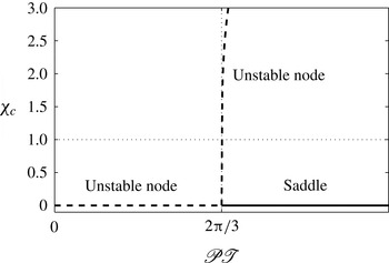
Bifurcation plot for
 $\mathscr{P}\mathscr{T}$
versus the
 ${\it\chi}_{c}$
values of the two stationary points. Here the
 ${\it\chi}_{c}$
value of the non-zero point has been computed with
 $\mathscr{T}=2$
.

Summary of the position and behaviour of the two relevant stationary points.

The stationary points
 $({\it\chi}_{c},{\it\alpha}_{c})$
are found by setting
 $\text{d}{\it\alpha}/\text{d}{\it\tau}=0$
and
 $\text{d}{\it\chi}/\text{d}{\it\tau}=0$
in (3.11) and (3.12), which after some manipulation gives a quintic polynomial in
 ${\it\alpha}_{c}$
, the solutions of which are straightforward to obtain. Of these solutions only those that are purely real and lie in the fibre drawing region are relevant to this analysis. There are two such values of
 ${\it\alpha}_{c}$
and these are given in table 1 along with the corresponding values of
 ${\it\chi}_{c}$
. Note that the second of these points may be complex, meaning that a bifurcation exists since this point is only purely real for
 $\mathscr{P}\mathscr{T}>2{\rm\pi}/3$
. The bifurcation point is displayed in figure 2 where the purely real
 ${\it\chi}_{c}$
values of the two stationary points in table 1 are displayed over a range of
 $\mathscr{P}\mathscr{T}$
values; here the
 ${\it\chi}_{c}$
value for the second of these points has been calculated with
 $\mathscr{T}=2$
. This second point only lies in the fibre drawing region when
 ${\it\chi}_{c}<1$
, as indicated by the horizontal dotted line in figure 2, and this only occurs for a small range of
 $\mathscr{P}\mathscr{T}$
values immediately after the bifurcation point.
The behaviour of trajectories near the stationary points is characterised via an eigenvalue analysis of (3.16) and (3.17). These behaviours are summarised in table 1 and are indicated by solid and dashed lines in figure 2. The eigenvector for the stationary point at the origin which is directed towards the fibre drawing region is relevant to the discussion here and is given locally by
 $$\begin{eqnarray}{\it\alpha}_{s}({\it\chi})=\frac{c_{1}-1}{6\mathscr{T}}{\it\chi},\quad \text{with }c_{1}=\sqrt{1+\frac{9}{2{\rm\pi}}\mathscr{P}\mathscr{T}}.\end{eqnarray}$$
Where this point is an unstable node, trajectories in this direction move away from the origin; where the origin is a saddle point,
 ${\it\alpha}_{s}({\it\chi})$
approximates the stable separatrix of this saddle.
The turning points of the trajectories lie at the points where (3.16) and (3.17) are separately equal to zero (equivalent to the nullclines where
 $\text{d}{\it\alpha}/\text{d}{\it\chi}=0$
and
 $\text{d}{\it\chi}/\text{d}{\it\alpha}=0$
, respectively). These turning points occur at
 $$\begin{eqnarray}{\it\chi}=6\mathscr{T}{\it\alpha},\end{eqnarray}$$
which in the
 $({\it\chi},{\it\alpha})$
plane is equivalent to
 $\text{d}{\it\chi}/\text{d}{\it\alpha}=0$
, and
 $$\begin{eqnarray}{\it\chi}=\frac{4{\rm\pi}{\it\alpha}}{(1-{\rm\pi}^{2}{\it\alpha}^{4})\mathscr{P}},\end{eqnarray}$$
which is equivalent to
 $\text{d}{\it\alpha}/\text{d}{\it\chi}=0$
.
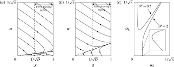
Plot of trajectories in the
 $({\it\chi},{\it\alpha})$
plane, for
 $\mathscr{T}=2$
, where the origin is (a) an unstable node for
 $\mathscr{P}=0.5$
or (b) a saddle for
 $\mathscr{P}=2$
; the arrows indicate the direction of increasing
 ${\it\tau}$
, the dotted lines are turning points in the trajectories, the angled dashed line is the linear approximation of the separatrix and the vertical dashed line is at
 ${\it\chi}=1/\sqrt{D}=0.475$
. (Note that this is an unrealistically small value of
 $D$
, which has been selected for illustrative purposes since a realistic value of this parameter would place the dashed line at the left edge of the figure, obscuring the intersection between the dashed line and some of the trajectories.) The feasible values for
 ${\it\alpha}_{0}$
and
 ${\it\alpha}_{L}$
are shown in (c) for the two values of
 $\mathscr{P}$
. The inset plot is a detail of the portion of the
 $\mathscr{P}=2$
curve near
 ${\it\alpha}_{L}=0$
(fibre explosion) indicated by the dashed lines, showing the non-uniqueness of the solutions near that value; here the inset axes span
 $2.5\times 10^{-5}$
in
 ${\it\alpha}_{0}$
with
 $0<{\it\alpha}_{L}<6\times 10^{-2}$
, so that the inset curve is magnified more in the horizontal than in the vertical direction.

Some example trajectories in the
 $({\it\chi},{\it\alpha})$
phase plane for
 $\mathscr{T}=2$
are shown in figure 3(a,b) for
 $\mathscr{P}=0.5$
and
 $2$
, respectively. These values are either side of the bifurcation displayed in figure 2, so that in figure 3(a) the origin is an unstable node (where, effectively, in this regime, surface tension dominates pressurisation), and for the larger
 $\mathscr{P}$
value in figure 3(b) the origin is a saddle point (a regime where pressurisation dominates surface tension). The turning points given by (3.19) and (3.20) are displayed as dotted lines and
 ${\it\alpha}_{s}({\it\chi})$
from (3.18) is shown as an angled dashed line (obscured by the trajectories in figure 3
a, but visible near the origin in figure 3
b).
A solution to the fibre drawing problem consists of the part of a trajectory that spans from
 ${\it\chi}=1$
to
 ${\it\chi}=1/\sqrt{D}$
in a direction of increasing
 ${\it\tau}$
, as indicated by the arrows in figure 3. As can be seen in figure 3(a) not all trajectories have a part that constitutes such a solution. Thus, the range of feasible values for preform geometry
 ${\it\alpha}_{0}={\it\alpha}(1)$
and fibre geometry
 ${\it\alpha}_{L}={\it\alpha}(1/\sqrt{D})$
for a particular choice of draw parameters (in this case
 $D$
,
 $\mathscr{T}$
and
 $\mathscr{P}$
) that correspond to valid solutions is potentially restricted.
The feasible values of
 ${\it\alpha}_{0}$
and
 ${\it\alpha}_{L}$
for the two values of
 $\mathscr{P}$
are shown in figure 3(c), where each point on these curves corresponds to a valid solution. In both cases the feasible values of
 ${\it\alpha}_{0}$
do not extend over the full range of values that are possible in principle (
 $0<{\it\alpha}_{0}<1/\sqrt{{\rm\pi}}$
, corresponding to
 $1>{\it\rho}_{0}>0$
), showing that there are no feasible fibre geometries for this choice of draw parameters if the preform has a hole that is either too small or too big. For
 $\mathscr{P}=2$
the full physically valid range of
 ${\it\alpha}_{L}$
is feasible, but for
 $\mathscr{P}=0.5$
this is not the case. For instance, at this smaller value of pressure, fibre explosion (where
 ${\it\alpha}_{L}=0$
at
 ${\it\chi}=1/\sqrt{D}$
) does not occur, whereas it is possible for the larger value of pressure. As shown on the inset in figure 3(c), there is some non-uniqueness for the larger value of pressure, where for a very small range of
 ${\it\alpha}_{0}$
near the value for fibre explosion it is possible to obtain two different values of
 ${\it\alpha}_{L}$
.
Identifying the point of fibre explosion is of practical interest, since in an experiment this is a catastrophic event. As was seen in figure 3, fibre explosion only occurs when the origin is a saddle point and
 ${\it\alpha}_{0}$
is below some critical value. This value is well approximated by the intersection of
 ${\it\alpha}_{s}({\it\chi})$
and
 ${\it\chi}=1$
, since explosion occurs for trajectories that lie below the separatrix, which, it can be shown, lies below the line
 ${\it\alpha}_{s}({\it\chi})$
. Thus, the criterion for explosion is given as
 ${\it\alpha}_{0}<{\it\alpha}_{s}(1)$
, which may be rewritten in terms of the pressurisation to give
 $$\begin{eqnarray}\mathscr{P}>\frac{8{\rm\pi}}{3}{\it\alpha}_{0}(3\mathscr{T}{\it\alpha}_{0}+1).\end{eqnarray}$$
As stated above, this criterion effectively indicates when a trajectory starting at
 ${\it\alpha}_{0}$
lies below the stable separatrix, assuming that the separatrix is well approximated by the linear expression given in (3.18), and this assumption is justified for typical values of the fibre drawing parameters. Note that this criterion is different in character to the criterion proposed by Fitt et al. (Reference Fitt, Furusawa, Monro, Please and Richardson2002) for fibres with a small-diameter channel. That criterion is equivalent to
 ${\it\alpha}^{\prime }(1)>0$
, in the notation of this paper, and posits that an initial expansion of the hole at the preform end of the neck-down will lead to explosion of the fibre. This does not account for the situation, often seen experimentally, where an initial increase in aspect ratio due to the pressurisation is followed by a decrease in aspect ratio as the glass is stretched to the dimensions of a fibre and surface tension becomes dominant; that is, an initial increase in the aspect ratio of the tube is not necessarily catastrophic. Additionally, our criterion makes no assumptions about the relative diameter of the internal channel or the magnitude of surface tension. For convenience, the criterion (3.21) is rewritten in terms of dimensional variables in (1.5).
Similarly, we now propose a criterion for hole closure, where
 ${\it\alpha}_{L}=1/\sqrt{{\rm\pi}}$
. We use (3.15) to obtain the first three terms in a Taylor series expansion of
 ${\it\alpha}({\it\chi})$
about the point
 $(1/\sqrt{D},1/\sqrt{{\rm\pi}})$
. This expansion is then evaluated at
 $(1,{\it\alpha}_{0})$
and rearranged to obtain the criterion on pressure, namely that hole closure occurs for
 $$\begin{eqnarray}\mathscr{P}<\frac{a^{2}\sqrt{D}}{9(D-1)}\left(a({\it\alpha}_{0}-1/\sqrt{{\rm\pi}})+3(\sqrt{D}-1)\right)+\frac{2}{3}{\rm\pi}\sqrt{D}\left(1+3\frac{\sqrt{D}}{\sqrt{{\rm\pi}}}\mathscr{T}\right),\end{eqnarray}$$
with
 $a=-\sqrt{{\rm\pi}}+6\mathscr{T}\sqrt{D}$
. As with the proposed explosion criteria, (3.22) is straightforward to implement in an experimental setting since it simply involves evaluating an expression of easily interpreted draw and geometry parameters. An expression in terms of dimensional quantities is obtained by substituting
 $\mathscr{P}=p_{H}\sqrt{S_{0}}/{\it\gamma}$
and
 $\mathscr{T}={\it\sigma}/(6{\it\gamma}\sqrt{S_{0}})$
.
3.2. Forward and inverse problems in dimensional variables
Trajectories of the type discussed in § 3.1 are now considered over a range of tensions and pressurisations as we apply our model to the forward and inverse problems. The forward problem predicts the final fibre for a known preform and a set of drawing parameters, while the inverse problem involves running the model backwards in
 ${\it\tau}$
to determine the shape of a preform and the draw parameters required to give a specified final fibre.
It is appropriate to discuss the solution to these problems in terms of the dimensional draw parameters, namely
 $$\begin{eqnarray}\displaystyle & \displaystyle p_{H}=\frac{{\it\gamma}}{\sqrt{S_{0}}}\mathscr{P}, & \displaystyle\end{eqnarray}$$
 $$\begin{eqnarray}\displaystyle & \displaystyle {\it\sigma}=6{\it\gamma}\sqrt{S_{0}}\mathscr{T}, & \displaystyle\end{eqnarray}$$
 $$\begin{eqnarray}\displaystyle & \displaystyle \frac{{\it\mu}_{0}}{L}=\frac{{\it\gamma}}{U_{0}\sqrt{S_{0}}}\frac{1}{{\it\gamma}^{\ast }}, & \displaystyle\end{eqnarray}$$
 $\mathscr{P}$
and
 $\mathscr{T}$
, given in (3.13) and (3.14). Thus, knowledge of
 ${\it\gamma}^{\ast }$
outside of these ratios is only necessary if the quantity
 ${\it\mu}_{0}/L$
is of interest.
Six parameters are required to completely describe either the forward or inverse problem: the initial and final geometry parameters
 ${\it\rho}_{0}$
and
 ${\it\rho}_{L}$
, the draw ratio
 $D$
, the scaled surface tension
 ${\it\gamma}^{\ast }$
and the two ratios of fibre tension and hole pressurisation to surface tension,
 $\mathscr{T}$
and
 $\mathscr{P}$
. Note the last three of these parameters directly relate to physical quantities via (3.23)–(3.25), which makes it straightforward to choose physically meaningful values of these parameters. When solving the system it is necessary to specify four of the six parameters, with the model output determining the other two (typically
 ${\it\gamma}^{\ast }$
and either
 ${\it\rho}_{L}$
or
 ${\it\rho}_{0}$
for the forward or inverse problem, respectively). Additionally, the total deformation time
 ${\it\tau}_{L}$
is recorded since this quantity is a useful measure of the competition between the stretching and the effects of surface tension and pressurisation.
The surface tension parameter
 ${\it\gamma}^{\ast }$
is determined via (2.20), which is straightforward to evaluate once we have found
 ${\it\chi}({\it\tau})$
from the model (and have a known viscosity profile
 ${\it\mu}^{\ast }(x)$
, which for all the examples shown here is chosen to be
 ${\it\mu}^{\ast }(x)=1$
). If we are concerned with knowing the geometry of the solution at each point throughout the neck-down region then we must additionally solve for the scaled axial coordinate
 $x$
from (2.19), which positions the solutions from the Lagrangian time coordinate
 ${\it\tau}$
in physical space. When
 ${\it\mu}^{\ast }(x)=1$
it is convenient to solve (2.19) for a scaled coordinate
 ${\it\gamma}^{\ast }x$
, namely
 $$\begin{eqnarray}\frac{\text{d}({\it\gamma}^{\ast }x)}{\text{d}{\it\tau}}=\frac{1}{{\it\chi}},\end{eqnarray}$$
where
 ${\it\gamma}^{\ast }$
is then chosen such that
 $x({\it\tau}_{L})=1$
when
 ${\it\chi}({\it\tau}_{L})=1/\sqrt{D}$
.
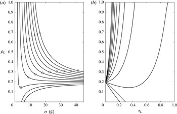
(a) Contours of
 ${\it\rho}_{L}$
against fibre tension
 ${\it\sigma}$
with channel pressurisations
 $p_{H}=0,200,\ldots ,2000$
Pa (bottom to top) for the forward problem with
 ${\it\rho}_{0}=0.2$
. (b) Contours of
 ${\it\rho}_{L}$
against
 ${\it\tau}_{L}$
over a range of constant
 $p_{H}=0,200,\ldots ,2000$
Pa (bottom to top) for the forward problem with
 ${\it\rho}_{0}=0.2$
. The remaining parameters for the displayed solutions are
 $D=3000$
,
 $S_{0}=7.54\times 10^{-5}~\text{m}^{2}$
,
 $U_{0}=1.4~\text{m min}^{-1}$
and
 ${\it\gamma}=0.23~\text{N}~\text{m}^{-1}$
. The crosses in (a) indicate the critical value of tension predicted by (3.21) (for the larger pressures where explosion is possible at low tension) or by (3.22) (for
 $p_{H}=0$
and 200 Pa where hole closure may occur). The circles are for the explosion criterion given by Fitt et al. (Reference Fitt, Furusawa, Monro, Please and Richardson2002) for an initially small hole.

The solutions to a suite of forward problems are displayed in figure 4, where each point along these curves represents a solution for a choice of drawing parameters. These were obtained by the numerical solution (using MATLAB) of the governing equations (3.11) and (3.12) for increasing
 ${\it\tau}$
. The aspect ratio of the preform is
 ${\it\rho}_{0}=0.2$
, corresponding to
 ${\it\alpha}_{0}\approx 0.4607$
, and the draw ratio is fixed at
 $D=3000$
. The draw parameters
 ${\it\sigma}$
and
 $p_{H}$
are specified (via
 $\mathscr{T}$
and
 $\mathscr{P}$
) over the range indicated in the figure. The surface tension is
 ${\it\gamma}=0.23~\text{N}~\text{m}^{-1}$
, the cross-sectional area of the preform is
 $S_{0}=7.54\times 10^{-5}~\text{m}^{2}$
and the feed speed is
 $U_{0}=1.4~\text{m}~\text{min}^{-1}$
. Having specified these parameters, the numerical method will solve for the fibre geometry
 ${\it\rho}_{L}$
(shown in figure 4
a),
 ${\it\gamma}^{\ast }$
and the total deformation time
 ${\it\tau}_{L}$
(the latter is shown in figure 4
b).
The solutions for no applied pressure
 $(p_{H}=0)$
are, as expected, identical to those of Stokes et al. (Reference Stokes, Buchak, Crowdy and Ebendorff-Heidepriem2014): for low fibre tension the surface tension dominates and acts to close the geometry, while at higher fibre tension, where surface tension has less opportunity to act,
 ${\it\rho}_{L}$
approaches the initial value
 ${\it\rho}_{0}$
. Not surprisingly, applying active pressurisation, holding other parameters constant, will ‘open’ the geometry (that is, increase
 ${\it\rho}_{L}$
from the unpressurised value). For smaller tension values it is clear that application of pressure will, in general, result in fibre explosion, i.e.
 ${\it\rho}_{L}=1$
. Note that in the regime of small tension most of the
 $({\it\sigma},{\it\rho}_{L})$
curves are nearly vertical and the solutions are very sensitive to the choice of tension
 ${\it\sigma}$
; a small change in tension will be the difference between a successful fibre and explosion. However, for sufficiently small pressure,
 $p_{H}$
, surface tension will prevent fibre explosion or even win and completely close the channel.
Figure 4(b) shows the competition between surface tension and pressurisation in terms of the deformation time
 ${\it\tau}_{L}$
. If
 ${\it\rho}_{L}<{\it\rho}_{0}$
is desired then application of pressure will increase the time
 ${\it\tau}_{L}$
needed to achieve this, or even make it impossible. If
 ${\it\rho}_{L}>{\it\rho}_{0}$
is desired then the pressure
 $p_{H}$
must be above some threshold value sufficient to overcome surface tension (dependent on the initial geometry), and the deformation time
 ${\it\tau}_{L}$
needed reduces as
 $p_{H}$
increases above this threshold;
 ${\it\tau}_{L}$
also becomes very sensitive to
 $p_{H}$
as
 $p_{H}$
becomes large.
The critical tension values from the criteria for explosion (3.21) and hole closure (3.22) at each choice of pressurisation are shown as crosses on the solution curves in figure 4(a); here the crosses on the
 $p_{H}=0$
and 200 Pa curves are from the closure criterion and the crosses on the remaining curves are from the explosion criterion. The circles are the critical values from the criterion given by Fitt et al. (Reference Fitt, Furusawa, Monro, Please and Richardson2002) for the expansion of an initially small hole. Recall that both explosion criteria are approximate and predict the value of pressurisation
 $p_{H}$
for which explosion is likely to occur given the other draw and geometry parameters or, as shown in figure 4(a), they may be used to predict the critical value of the fibre tension below which explosion is likely to occur given the pressure
 $p_{H}$
and other draw and geometry parameters. As a result, in figure 4(a) the
 ${\it\rho}_{L}$
values that correspond to the predicted critical values of
 ${\it\sigma}$
are less than
 ${\it\rho}_{L}=1$
. The predictions from (3.21) give a lower critical tension value at all values of pressure
 $p_{H}$
compared to that given by Fitt, so that using our criterion with, for example,
 $p_{H}=2000$
Pa allows a much wider range of
 ${\it\rho}_{L}$
, which more accurately reflects the feasible geometries given by the numerical solution. Fitt et al. (Reference Fitt, Furusawa, Monro, Please and Richardson2002) also proposed a criterion for hole closure (not shown in figure 4
a) that predicts hole closure at tensions below the value indicated by the numerical solution. Our closure criterion (3.22) tends to slightly overestimate the critical tension associated with hole closure, which is preferable to the Fitt criterion since underestimating tension will result in a fibre with no air channel.
There are circumstances where the choice of tension to achieve a certain geometry
 ${\it\rho}_{L}$
with a given pressure
 $p_{H}$
is not unique. This is seen on the
 $({\it\sigma},{\it\rho}_{L})$
curve for
 $p_{H}=400$
Pa. Here there is a local minimum in the curve and either side of this value there are two possible tension values for each choice of
 ${\it\rho}_{L}<{\it\rho}_{0}$
, where the low-tension solution corresponds to a larger
 ${\it\tau}_{L}$
value, i.e. a longer deformation time.
(a) Contours of
 ${\it\rho}_{0}$
against fibre tension
 ${\it\sigma}$
with channel pressurisations
 $p_{H}=0,100,\ldots ,1000$
Pa (top to bottom) for the inverse problem with
 ${\it\rho}_{L}=0.6$
. (b) Contours of
 ${\it\rho}_{0}$
against
 ${\it\tau}_{L}$
over a range of constant
 $p_{H}=0,100,\ldots ,1000$
Pa (top to bottom) for the inverse problem with
 ${\it\rho}_{L}=0.6$
. The remaining parameters for the displayed solutions are
 $D=3000$
,
 $S_{0}=7.54\times 10^{-5}~\text{m}^{2}$
,
 $U_{0}=1.4~\text{m min}^{-1}$
and
 ${\it\gamma}=0.23~\text{N m}^{-1}$
.

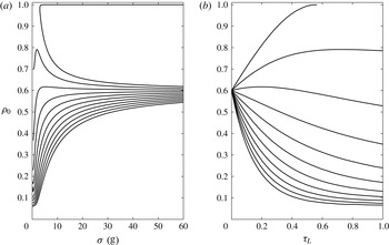
To solve the inverse problem and find a preform and draw parameters to yield a desired fibre, it is easiest to use (3.15) and solve this ‘backwards’, from
 ${\it\chi}=1/\sqrt{D}$
to
 ${\it\chi}=1$
, to find the preform geometry
 ${\it\rho}_{0}$
. Some solutions to the inverse problem are shown in figure 5, where preform geometry
 ${\it\rho}_{0}$
is plotted against fibre tension
 ${\it\sigma}$
(figure 5
a) and deformation time
 ${\it\tau}_{L}$
(figure 5
b) for a range of pressurisations
 $p_{H}$
. The draw ratio is again set at
 $D=3000$
(dictated by the desired change in cross-sectional area from preform to fibre) and the geometry of the final fibre is set at
 ${\it\rho}_{L}=0.6$
.
For the unpressurised (
 $p_{H}=0$
) case two
 ${\it\rho}_{0}$
solutions exist for each value of
 ${\it\sigma}$
; one solution approaches the geometry of the fibre at high tension and the other approaches
 ${\it\rho}_{0}=1$
, corresponding to very thin-walled preforms. These latter solutions have been computed using (3.16) and (3.17), since
 ${\it\chi}$
is not monotonically decreasing. The existence of these solutions is mathematically interesting, but in practice preforms with very thin walls are impossible to manufacture and only the smaller
 ${\it\rho}_{0}$
is a feasible option. Aside from the case
 $p_{H}=0$
, non-uniqueness of
 ${\it\rho}_{0}$
is seen for
 $p_{H}>0$
only over a finite range of tensions. In fact, with reference to our earlier analysis of the
 $({\it\chi},{\it\alpha})$
plane in § 3.1, we have non-uniqueness for
 $\mathscr{PT}<2{\rm\pi}/3$
, i.e. from (3.23)–(3.25),
 $(p_{H}/{\it\gamma})({\it\sigma}/{\it\gamma})<4{\rm\pi}$
, when the origin in the
 $({\it\chi},{\it\alpha})$
plane is an unstable node; this is most easily seen in the curve for
 $\mathscr{P}=0.5$
in figure 3(c). Thus for
 $p_{H}$
significantly above zero the tension must be near zero, which is completely impractical. For the values of
 $p_{H}>0$
used in figure 5(a) the curves have not been computed for such small values of
 ${\it\sigma}$
(since no feasible solutions exist there) and no non-uniqueness is seen. Nevertheless, for a non-zero choice of
 $p_{H}$
there are two choices of
 ${\it\rho}_{0}$
at sufficiently low tension, corresponding to thin-walled and thick-walled preforms.
In general, for a given fibre geometry
 ${\it\rho}_{L}$
, the aspect ratio of the required preform
 ${\it\rho}_{0}$
reduces as the pressure
 $p_{H}$
increases, holding other draw parameters constant. For small values of pressurisation (for instance
 $p_{H}=100$
Pa) the surface tension will still dominate so that the preform geometry must have a larger ratio between the inner and outer boundaries than that of the fibre. The larger values of pressurisation here considered all lead to preforms whose geometries are more closed than the desired fibre, with pressurisation overcoming surface tension. Additionally there is some non-uniqueness present in some of these pressurised solutions (namely for
 $p_{H}=100,200$
Pa), where identical preforms may be drawn at two different tension values,
 ${\it\sigma}$
, to give the same fibre. Note that the solutions at lower tensions are associated with a viscosity that is too low for a fibre to be drawn, where typically glass is malleable enough for fibre drawing when the viscosity
 ${\it\mu}_{0}$
is in the range
 $\mathit{O}(10^{4}~\text{Pa}~\text{s})<{\it\mu}_{0}<\mathit{O}(10^{5}~\text{Pa}~\text{s})$
.
The termination of the curves for low values of tension
 ${\it\sigma}$
is associated with the influence of an unstable node on trajectories in the fibre drawing region. For
 $p_{H}=100$
and 200 Pa the curves terminate at the value of
 ${\it\sigma}$
at which the stationary point at the origin changes in character from a saddle to an unstable node; trajectories sufficiently near the origin are then ‘attracted’ to the unstable node as they are run backwards in
 ${\it\tau}$
and so do not reach
 ${\it\chi}=1$
. The curves for the remaining values of pressurisation terminate when the second stationary point given in table 1 (also an unstable node) enters the fibre drawing region. Again, as the trajectories near this point they are attracted to it rather than reaching
 ${\it\chi}=1$
, and so do not constitute a valid fibre drawing solution. These low tensions correspond to viscosities that are at least an order of magnitude smaller than is required for fibre drawing.
(a) Comparison between the model output (circles) and experimental data (crosses, with
 $\pm 5\,\%$
measurement error) for the fibre geometry
 ${\it\rho}_{L}$
against the applied pressure
 $p_{H}$
. (b) The measured fibre tension versus the applied pressure
 $p_{H}$
, shown as crosses with a
 $\pm$
2 g measurement error. The remaining parameters are
 ${\it\rho}_{0}=0.17$
,
 $U_{0}=1.4~\text{mm}~\text{min}^{-1}$
,
 $U_{L}=5.6~\text{m}~\text{min}^{-1}$
,
 $D=4000$
and
 ${\it\gamma}=0.23~\text{N}~\text{m}^{-1}$
.

3.3. Comparison with experiment
Experimental validation of the above model for drawing annular fibres with channel pressurisation is ongoing. The results from an initial experiment are extremely promising and these are presented here as confirmation that pressurisation has been included correctly in the model. This experiment involved drawing to fibre an annular preform made of F2 glass, a lead-silicate glass from the Schott Glass Company (2015), which has previously been used in experimental fibre drawing studies as a less expensive alternative to pure silica glass (Ruan et al. Reference Ruan, Schartner, Ebendorff-Heidepriem, Hoffmann and Monro2007; Monro et al. Reference Monro, Warren-Smith, Schartner, François, Heng, Ebendorff-Heidepriem and Afshar2010).
The preform geometry, which was measured prior to drawing, was
 ${\it\rho}_{0}=0.17$
. The furnace temperature was set at
 $T=900\,^{\circ }\text{C}$
, the preform feed speed was
 $U_{0}=1.4~\text{mm}~\text{min}^{-1}$
and the surface tension for F2 glass is taken to be
 ${\it\gamma}=0.23~\text{N}~\text{m}^{-1}$
(see Boyd et al.
Reference Boyd, Ebendorff-Heidepriem, Monro and Munch2012). In the experiment the fibre was initially drawn without pressurisation (that is with
 $p_{H}=0$
) with a draw speed of
 $U_{L}=5.6~\text{m}~\text{min}^{-1}$
selected to achieve an outer fibre diameter of approximately
 $160~{\rm\mu}\text{m}$
, thus the draw ratio was
 $D=4000$
. Over the course of the experiment pressurisation was increased in increments of 1000 Pa up to a maximum of
 $p_{H}=4000$
Pa. After each change in pressurisation the fibre was drawn for around 30 m to ensure a steady state had been reached.
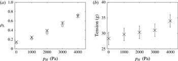
The experimental values for the fibre geometry
 ${\it\rho}_{L}$
are shown as crosses in figure 6(a). At each pressurisation the
 ${\it\rho}_{L}$
value is the average of three measurements taken from the portion of the fibre drawn at the steady state. There is excellent agreement between the experimental values and the model output, shown as circles in figure 6(a), with the model accurately capturing the expansion of the geometry as the pressurisation is increased.
A key point of difference between this experiment and previous studies (the experimental results presented in Fitt et al. (Reference Fitt, Furusawa, Monro, Please and Richardson2002), for instance) is that the equipment used here is capable of measuring the fibre tension. As demonstrated in § 2 and in Stokes et al. (Reference Stokes, Buchak, Crowdy and Ebendorff-Heidepriem2014), fibre tension is crucial in determining the fibre geometry, and by measuring this quantity it is possible to avoid the need to know about the temperature or viscosity of the glass, which are not measurable during a fibre draw. As shown in figure 6(b), the fibre tension increased slightly throughout the draw as pressurisation was increased. This is due in part to the fibres with a larger
 ${\it\rho}_{L}$
also having a larger outer diameter, which leads to a lower glass temperature, owing to the lower thermal mass associated with the relatively thinner walls in the neck-down.
The preform used in this experiment was produced by an extrusion process and features a slight taper in outer diameter, as is typical of preforms that are produced in this way due to the gravity stretching that occurs during extrusion. As a result of this slight variation, it is not possible to know precisely the diameter of the preform that corresponds to a given point on the fibre; this is crucial since the preform area
 $S_{0}$
appears in the non-dimensionalisation of fibre tension (2.13). Since it is not possible to directly measure this area, we instead compute
 $S_{0}$
from the measured fibre area
 $S_{L}$
, via (2.1) and (2.10), so that
 $$\begin{eqnarray}S_{0}=DS_{L},\end{eqnarray}$$
where both the fibre area
 $S_{L}$
and the draw ratio
 $D$
are known accurately.
4. Case study: multi-hole fibres
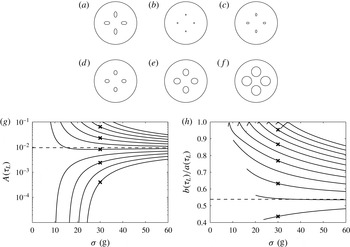
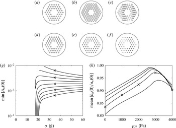
The annular case of the previous section is the simplest possible geometry containing an internal channel. Although this fundamental case is instructive, the modelling approach is capable of handling much more complicated cross-sectional geometries. Two such cases are considered here: a forward problem drawing a preform with four channels and an inverse problem to draw a fibre with an array of 54 channels. The cross-sectional shape of the channels is assumed to be elliptical, in line with experimental observations of the deformation of circular channels (see, for instance, Stokes et al. Reference Stokes, Buchak, Crowdy and Ebendorff-Heidepriem2014; Buchak et al. Reference Buchak, Crowdy, Stokes and Ebendorff-Heidepriem2015). Imposing such a restriction has the benefit of avoiding the stability issues associated with the ill-posed nature of the inverse problem, as discussed in Stokes et al. (Reference Stokes, Buchak, Crowdy and Ebendorff-Heidepriem2014). This restriction also means that the highly efficient elliptical pore model of Buchak et al. (Reference Buchak, Crowdy, Stokes and Ebendorff-Heidepriem2015) can be used to solve for the flow in the cross-plane. This Stokes-flow free-boundary problem may now feature many interfaces and a flow domain that is more complicated than the simple case of § 3, and this method makes the solution of this difficult problem computationally tractable.
The method of Buchak et al. (Reference Buchak, Crowdy, Stokes and Ebendorff-Heidepriem2015) generalises the elliptical pore model (EPM) approach of Crowdy (Reference Crowdy2004) by including an external boundary so that the method is applicable to fibre drawing. The key assumptions behind the EPM are that the cross-sectional shapes of the channels are elliptical for all time, and that the channels do not lie too close together in the cross-plane. As demonstrated in Buchak et al. (Reference Buchak, Crowdy, Stokes and Ebendorff-Heidepriem2015), the solutions from this asymptotic approach are in very close agreement with results from a full numerical solution that does not impose these restrictions.
The inclusion of pressurisation in the internal channels is described in Buchak et al. (Reference Buchak, Crowdy, Stokes and Ebendorff-Heidepriem2015) but not fully implemented, and none of the examples in that work include pressurised channels. As with the annular example in § 3, the inclusion of pressurisation requires the simultaneous solution of the cross-plane and axial models. The relevant governing equations are given in § 5 of Buchak et al. (Reference Buchak, Crowdy, Stokes and Ebendorff-Heidepriem2015) and these are reused here, via a publicly available MATLAB implementation of that work (Buchak & Crowdy Reference Buchak and Crowdy2014), with the addition of the two differential equations governing the axial stretching (2.17) and (2.18) and, for completeness, the relation between the physical position
 $x$
of the cross-section and reduced time
 ${\it\tau}$
(2.19). The relevant system of differential equations from Buchak et al. (Reference Buchak, Crowdy, Stokes and Ebendorff-Heidepriem2015) is reported below and we refer interested readers to that work for full details of the derivation.
In summary, the parameters that describe the cross-sectional geometry are the radius of the outer boundary
 $R({\it\tau})$
, the position in the complex plane of each channel in the cross-section
 $\mathscr{Z}_{n}({\it\tau})$
, plus real parameters
 ${\it\alpha}_{n}({\it\tau})$
and complex parameters
 ${\it\beta}_{n}({\it\tau})$
, for
 $n=1\ldots N$
, which describe the size, aspect ratio and rotation of each of the
 $N$
elliptical channels. The
 ${\it\alpha}_{n}$
and
 ${\it\beta}_{n}$
relate to the semi-major axis
 $a_{n}$
and semi-minor axis
 $b_{n}$
of the
 $n$
th channel via
 $$\begin{eqnarray}a_{n}={\it\alpha}_{n}+|{\it\beta}_{n}|,\quad b_{n}={\it\alpha}_{n}-|{\it\beta}_{n}|\end{eqnarray}$$
and the area of the channel is
 $$\begin{eqnarray}A_{n}={\rm\pi}a_{n}b_{n}={\rm\pi}({\it\alpha}_{n}^{2}-|{\it\beta}_{n}|^{2}).\end{eqnarray}$$
In the following discussion the solution will sometimes be discussed in terms of the area of the channels as well as the ratio between the semi-major and semi-minor axes
 $a_{n}/b_{n}$
.
The differential equations governing the evolution of the channel positions
 $\mathscr{Z}_{n}$
, the channel geometry parameters
 ${\it\alpha}_{n}$
and
 ${\it\beta}_{n}$
and the outer boundary radius
 $R$
are
 $$\begin{eqnarray}\displaystyle & \displaystyle \overline{\frac{\text{d}{\mathcal{Z}}_{n}}{\text{d}{\it\tau}}}=-\mathop{\sum }_{j\neq n}\frac{{\it\lambda}_{j}\overline{({\mathcal{Z}}_{n}-{\mathcal{Z}}_{j})}}{2{\rm\pi}({\mathcal{Z}}_{n}-{\mathcal{Z}}_{j})^{2}}+\mathop{\sum }_{j\neq n}\frac{m_{j}}{2{\rm\pi}({\mathcal{Z}}_{n}-{\mathcal{Z}}_{j})}-\overline{\mathop{\sum }_{j\neq n}\frac{{\it\lambda}_{j}}{2{\rm\pi}({\mathcal{Z}}_{n}-{\mathcal{Z}}_{j})}}, & \displaystyle\end{eqnarray}$$
 $$\begin{eqnarray}\displaystyle & \displaystyle \frac{\text{d}{\it\alpha}_{n}}{\text{d}{\it\tau}}=-{\it\alpha}_{n}I_{n}(0)-\frac{1}{2}{\it\alpha}_{n}(p_{n}-\mathscr{P}^{(n)}{\it\chi}), & \displaystyle\end{eqnarray}$$
 $$\begin{eqnarray}\displaystyle & \displaystyle \frac{\text{d}{\it\beta}_{n}}{\text{d}{\it\tau}}=-{\it\beta}_{n}I_{n}(0)+\frac{1}{2}{\it\beta}_{n}(p_{n}-\mathscr{P}^{(n)}{\it\chi})+2\overline{k}_{n}{\it\alpha}_{n}+\text{i}{\it\omega}_{n}{\it\beta}_{n}, & \displaystyle\end{eqnarray}$$
 $$\begin{eqnarray}\displaystyle & \displaystyle \frac{\text{d}R}{\text{d}{\it\tau}}=\frac{\mathscr{M}}{2{\rm\pi}R}. & \displaystyle\end{eqnarray}$$
 ${\it\lambda}_{j}$
and
 $m_{j}$
are the strengths of the point stresslet and the point sink, respectively, located at the centre of the
 $j$
th channel. These determine the ambient pressure
 $p_{n}$
, linear strain rate
 $k_{n}$
and vorticity
 ${\it\omega}_{n}$
‘seen’ by the
 $n$
th channel in its far field.
 $\mathscr{M}$
is the sum of point sink strengths and
 $I_{n}(0)$
is an integral given in appendix B of Buchak et al. (Reference Buchak, Crowdy, Stokes and Ebendorff-Heidepriem2015). The pressure in the
 $n$
th channel is
 $\mathscr{P}^{(n)}$
and
 ${\it\chi}$
is the square root of the cross-sectional glass area (thus coupling this model to the axial flow model).
Additionally, it is worth noting that for a single, centred circular channel (namely the circular tube case of § 3) the elliptical pore model retrieves (3.10) exactly (see appendix C in Buchak et al. (Reference Buchak, Crowdy, Stokes and Ebendorff-Heidepriem2015) for this alternative derivation).
Two examples from Buchak et al. (Reference Buchak, Crowdy, Stokes and Ebendorff-Heidepriem2015) are reconsidered here with channel pressurisation included; these are a forward problem for a four-holed preform and an inverse problem for a fibre with a hexagonal array of channels. Although the model allows pressurisation to be specified on a per-channel basis, this is not practically possible with existing fibre drawing equipment, and so in both cases it will be assumed that
 $p^{(k)}=p_{H}$
for
 $k\neq 0$
and
 $p^{(0)}=0$
.
(a) Geometry of the four-hole preform; (b–f) fibre geometries obtained using a tension of 30 g with the given pressure
 $p_{H}$
((b) 0 Pa, (c) 200 Pa, (d) 400 Pa, (e) 600 Pa, (f) 800 Pa), corresponding to the crosses in (g,h); (g) contours of channel area
 $A({\it\tau}_{L})$
against fibre tension
 ${\it\sigma}$
with channel pressurisations
 $p_{H}=0,100,\ldots ,1000$
Pa (bottom to top); (h) contours of channel aspect ratio against fibre tension
 ${\it\sigma}$
with channel pressurisations
 $p_{H}=0,100,\ldots ,1000$
Pa (bottom to top). In (g,h) the horizontal dashed lines show the values of the respective parameters for the preform shown in (a). The remaining parameters for the displayed solutions are
 $D=3000$
,
 $S_{0}=3.03\times 10^{-4}~\text{m}^{2}$
,
 $U_{0}=1.4~\text{m min}^{-1}$
and
 ${\it\gamma}=0.23~\text{N m}^{-1}$
.

The geometry of the four-holed preform is shown in figure 7(a), where the four identically shaped elliptical channels are arranged in a symmetric pattern and the initial preform area is
 $S_{0}=3.03\times 10^{-4}~\text{m}^{2}$
(for a preform radius of 1 cm). The drawing of this preform was computed for a fixed draw ratio of
 $D=3000$
over a range of tensions and channel pressurisations with the surface tension parameter
 ${\it\gamma}=0.23~\text{N m}^{-1}$
. As in the annular case there is the possibility that surface tension will dominate and close the channels, or that the inclusion of too high a pressure will expand the channels to the point where their boundaries overlap.
In figure 7(g,h) the area
 $A({\it\tau}_{L})$
and aspect ratio
 $b({\it\tau}_{L})/a({\it\tau}_{L})$
of the channels of the drawn fibre, where both of these quantities are identical for each of the four channels so that the subscripts have been dropped, are plotted against tension
 ${\it\sigma}$
as curves of constant pressure (for
 $p_{H}=0\ldots 1000~\text{Pa}$
). The dashed lines here represent the initial values of these two quantities in the preform. The five crosses in each figure correspond to the five solutions displayed in figure 7(b–f), namely the fibre geometries that result from the preform being stretched with a tension of
 ${\it\sigma}=30\,\text{g}$
for
 $p_{H}=0$
, 200, 400, 600 and 800 Pa.
Where no pressurisation is applied the channels almost close due to the effect of surface tension and are slightly more elliptical than the initial configuration (figure 7
b). As the pressurisation is increased, the channels in the resulting fibres, as shown in figure 7(c–f), are much more open and more circular. For the case
 $p_{H}=800$
Pa shown in figure 7(f) the area of the channels is more than two orders of magnitude larger than in the unpressurised case and the channels are nearly circular in shape with an aspect ratio close to
 $b({\it\tau}_{L})/a({\it\tau}_{L})=1$
. As can be seen from figure 7(g,h), this is broadly the effect of increasing pressurisation for any tension, namely larger and more circular channels.
As tension
 ${\it\sigma}$
is increased, the geometry tends towards that of the preform, since both surface tension and pressurisation have less opportunity to act. At low tensions the solutions for small pressurisations are dominated by surface tension and the holes may even close completely. At larger pressurisations and low tension the pressure may expand the channels to the point where their boundaries overlap, analogous to the fibre explosion of the annular fibre. The switch between the two behaviours occurs here between
 $p_{H}=300$
and 400 Pa, which mirrors the type of behaviour seen for the annular case in, for instance, figure 4(a).
The termination of each of the curves in figure 7(h) corresponds to either the closure or overexpansion of the holes. Note that the tick on the end of the larger pressure curves represents a small region where the geometry is slightly elliptical, but at 90
 $^{\circ }$
to the original orientation in the preform. Such solutions only occur where boundaries are nearly overlapping and it is unclear whether these solutions are significant or an artifact of the elliptical pore model (which is expected to be inaccurate where the pores are too close together).
(a) Geometry of the fibre with a hexagonal array of channels; (b–f) preform geometries required when using a tension of 35 g with the given pressure
 $p_{H}$
((b) 0 Pa, (c) 1000 Pa, (d) 2000 Pa, (e) 3000 Pa, (f) 4000 Pa), corresponding to the crosses in (g,h); (g) contours of the minimum channel area
 $A_{n}(0)$
against fibre tension
 ${\it\sigma}$
with channel pressurisations
 $p_{H}=0,500,\ldots ,4000$
Pa (top to bottom); (h) contours of mean channel aspect ratio against channel pressurisation
 $p_{H}$
for fibre tensions
 ${\it\sigma}=30,35,40,45$
and
 $50$
g (bottom to top). The remaining parameters for the displayed solutions are
 $D=3000$
,
 $S_{0}=7.18\times 10^{-5}~\text{m}^{2}$
,
 $U_{0}=1.4~\text{m}~\text{min}^{-1}$
and
 ${\it\gamma}=0.23~\text{N}~\text{m}^{-1}$
.

Another case considered by Buchak et al. (Reference Buchak, Crowdy, Stokes and Ebendorff-Heidepriem2015) was an inverse problem to find the preform and draw parameters required to obtain the fibre configuration shown in figure 8(a), a hexagonal array of 54 small circular channels. Here the draw ratio is set at
 $D=3000$
, the area of the preform is
 $S_{0}=7.18\times 10^{-5}~\text{m}^{2}$
and the surface tension parameter is
 ${\it\gamma}=0.23~\text{N}~\text{m}^{-1}$
. Five preform configurations are shown in figure 8(b–f) where these correspond to the crosses in figure 8(g,h) and are for pressurisations of
 $p_{H}=0$
, 1000, 2000, 3000 and 4000 Pa with a tension of
 ${\it\sigma}=35$
g. As can be seen from these five configurations, the size of the preform channels decreases as the pressurisation is increased. The aspect ratio of the channels in the displayed configurations is difficult to see by eye. In general, compared to the unpressurised case, as pressurisation is increased the preform channels become more circular.
If too large a pressurisation is applied the model may give a preform where, as a consequence of solving backwards in
 ${\it\tau}$
, some channels are completely closed. Such a preform is not a valid solution to the inverse problem since it will not result in the desired fibre when drawn. To detect whether this has occurred we now consider the minimum area
 $A_{n}$
, across all channels
 $n=1,2,\ldots ,54$
, for each choice of parameters. These values of minimum area are shown against tension for a variety of pressurisations in figure 8(g).
Figure 8(h) shows the mean aspect ratio of the channels against pressurisation, where each curve is at a constant tension. This averaged quantity is of particular interest if a preform with circular channels is desired. This is of practical importance since preforms with circular channels can be fabricated through processes such as the stacking of many smaller capillary tubes or by drilling channels directly into a preform, as outlined by Monro & Ebendorff-Heidepriem (Reference Monro and Ebendorff-Heidepriem2006). For each choice of fibre tension in figure 8(h) there is a corresponding choice of pressurisation that gives a preform design where the mean aspect ratio reaches a maximum value close to 1. Thus, the curves in figure 8(h) demonstrate that it is possible, by carefully tuning the draw parameters, to achieve a situation where both the preform and fibre have circular channels (or at least very close to circular). Note that the gradient discontinuities in the curves in figure 8(b) are real, probably due to taking the average of the channel aspect ratios.
5. Conclusions
The key result of this paper has been to model the effect of channel pressurisation in the drawing of microstructured optical fibres by extending the work of Stokes et al. (Reference Stokes, Buchak, Crowdy and Ebendorff-Heidepriem2014). Where the pressurisation was assumed to be axially constant this led to a small but significant change to the model governing the flow in the cross-plane, namely an extra term in the dynamic boundary conditions, involving the cross-sectional area
 ${\it\chi}$
. This is a quantity from the axial model so that, in contrast to Stokes et al. (Reference Stokes, Buchak, Crowdy and Ebendorff-Heidepriem2014), the models for the axial and cross-plane flows become fully coupled and must be solved simultaneously.
Much of our work has focused on applying the model to a fibre with an annular cross-section. Although this is the simplest example of a fibre containing a holey structure, the effect of pressurisation on this case is extremely instructive, and many of the results for this simple geometry were echoed in the more complex geometries considered in § 5. As expected, including pressurisation opened the fibre geometry in the forward problem, and in the inverse problem it allowed preforms to be designed with geometries that featured smaller holes (and thus thicker walls) than in the unpressurised case. Another consequence of including pressurisation was that the non-uniqueness seen in the unpressurised inverse problem across the full range of fibre tension was restricted to a very small range of small (and impractical) fibre tension. Furthermore, new criteria for fibre explosion (3.21) and hole closure (3.22) have been obtained that are an improvement over similar criteria given by Fitt et al. (Reference Fitt, Furusawa, Monro, Please and Richardson2002). Here, our criteria do not assume that the hole geometry is small and our fibre explosion criterion is genuinely for explosion of the fibre at the end of the draw rather than for expansion at the start of the draw.
The excellent agreement between our model and the experimental results in § 3.3 for drawing an annular preform over a range of pressurisations is strong validation of the modelling approach and confirms that channel pressurisation has been included in the model correctly. Further experiments will include drawing fibres of more complex geometry with channel pressurisation.
The results for geometries with multiple channels presented in § 4 may be of interest to experimentalists. In drawing the preform with elliptical holes we saw that including pressurisation opened the channels in the fibre, and where sufficient pressurisation was applied the balance between surface tension and the pressurisation resulted in fibres with channels that were more circular than those in the preform. Similarly, in designing a preform to give a fibre with an array of small circular holes we saw that including pressurisation allowed for preform designs featuring holes that were close to circular; such designs are potentially easier to manufacture. An experimental study involving drawing preforms of this type with or without pressurisation would be of great interest to validate this modelling.
Acknowledgements
This research is supported by grant DP130101541 from the Australian Research Council and a Research Grant from the Leverhulme Trust in the United Kingdom. It was in part performed at the Optofab node of the Australian National Fabrication Facility utilizing Commonwealth and SA State Government funding. D.G.C. is partially supported by an Established Career Fellowship from the Engineering and Physical Sciences Research Council in the UK.
Appendix A. Derivation of the axial momentum equation
The axial momentum equation (2.12) is derived in a similar way to the equivalent expression in Cummings & Howell (Reference Cummings and Howell1999). Here we allow for pressurised internal channels and, although in the above sections it is assumed that the channels were held at constant pressures, for maximum generality we now permit axial variation in these pressurisations. As in Stokes et al. (Reference Stokes, Buchak, Crowdy and Ebendorff-Heidepriem2014) the effects of inertia and gravity are neglected. The relevant expression is then obtained by integrating and manipulating the first-order components in the slenderness parameter
 ${\it\epsilon}^{2}$
of the conservation of momentum equation and the
 $x$
-stress boundary condition on the interfaces (see Cummings & Howell (Reference Cummings and Howell1999) for full details of these equations). This yields a very similar expression to that given in appendix A of Cummings & Howell (Reference Cummings and Howell1999), namely
 $$\begin{eqnarray}(3{\it\mu}Su_{0x})_{x}=-\frac{1}{2}\frac{\partial }{\partial x}\iint _{S}({\rm\nabla}^{2}A)\,\text{d}y\,\text{d}z+\mathop{\sum }_{k=0}^{N}\oint _{G^{(k)}}\left(\frac{{\it\gamma}{\it\kappa}_{0}^{(k)}+p^{(k)}}{\Vert \boldsymbol{n}^{(k)}\Vert }G_{x}^{(k)}\right)\text{d}s,\end{eqnarray}$$
where
 $\boldsymbol{n}^{(k)}=G_{y}^{(k)}\boldsymbol{j}+G_{z}^{(k)}\boldsymbol{k}$
. The only difference between (A 1) and the version given in Cummings & Howell (Reference Cummings and Howell1999) is that in the above expression the second term on the right-hand side now features a balance between surface tension and the pressures
 $p^{(k)}(x)$
. This term is also now taken as a sum over all the boundaries
 $G^{(k)}=0$
, for
 $k=0,\ldots ,N$
. In the following expressions the total area of the cross-plane
 $S$
is taken to be
 $S=\mathscr{A}^{(0)}-\sum _{k=1}^{N}\mathscr{A}^{(k)}$
, that is the area enclosed by the outer boundary less the sum of the areas enclosed by the internal boundaries. Similarly, the total circumference is
 ${\it\Gamma}=\sum _{k=0}^{N}{\it\Gamma}^{(k)}$
, where
 ${\it\Gamma}^{(k)}$
is the length of the
 $k$
th boundary and the axial derivative of this quantity
 ${\it\Gamma}_{x}=\sum _{k=0}^{N}{\it\Gamma}_{x}^{(k)}$
is simply the sum of the derivatives of the individual boundary lengths.
The first term on the right-hand side of (A 1) involves an Airy stress function
 $A$
and full details of the manipulations involving this function are omitted for reasons of space. It is sufficient to state that, by treating the stress boundary conditions in the cross-plane as in § 3 of Cummings & Howell (Reference Cummings and Howell1999), we obtain
 $$\begin{eqnarray}\frac{\partial A}{\partial \hat{\boldsymbol{n}}^{(k)}}=-{\it\gamma}-p^{(k)}(y\boldsymbol{j}+z\boldsymbol{k})\boldsymbol{\cdot }\hat{\boldsymbol{n}}^{(k)},\end{eqnarray}$$
where
 $\hat{\boldsymbol{n}}^{(k)}$
is a unit vector normal to the interface
 $G^{(k)}=0$
. The area integral in the first term on the right-hand side of (A 1) may be rewritten as a contour integral via the divergence theorem, into which (A 2) is then substituted. The contour integrals of the various parts of the resulting expression may then be evaluated to give
 $$\begin{eqnarray}\iint _{S}({\rm\nabla}^{2}A)\,\text{d}y\,\text{d}z=-{\it\gamma}{\it\Gamma}-2p^{(0)}\mathscr{A}^{(0)}+2\mathop{\sum }_{k=1}^{N}p^{(k)}\mathscr{A}^{(k)}.\end{eqnarray}$$
Note that in manipulating the above expression care must be taken to correctly sign the normal vectors and the sub-parts of the area integral.
The second term on the right-hand side of (A 1) is evaluated as
 $$\begin{eqnarray}\mathop{\sum }_{k=0}^{N}\oint _{G^{(k)}}\left(\frac{{\it\gamma}{\it\kappa}_{0}^{(k)}+p^{(k)}}{\Vert \boldsymbol{n}^{(k)}\Vert }G_{x}^{(k)}\right)\text{d}s=-{\it\gamma}{\it\Gamma}_{x}-p^{(0)}\mathscr{A}_{x}^{(0)}+\mathop{\sum }_{k=1}^{N}p^{(k)}\mathscr{A}_{x}^{(k)}.\end{eqnarray}$$
This is obtained by noting that the part of this term involving surface tension and curvature is identical to that in Cummings & Howell (Reference Cummings and Howell1999) and their result is used here without rederivation. The part of (A 4) due to the pressurisations has been evaluated via a transport theorem given by Dewynne et al. (Reference Dewynne, Howell and Wilmott1994) (which is not restated here for brevity).
Finally, the expressions (A 3) and (A 4) are substituted back into (A 1) and the result may be slightly rearranged to give
 $$\begin{eqnarray}(3{\it\mu}Su_{0x})_{x}+\frac{1}{2}{\it\gamma}{\it\Gamma}_{x}-p_{x}^{(0)}\mathscr{A}^{(0)}+\mathop{\sum }_{k=1}^{N}p_{x}^{(k)}\mathscr{A}^{(k)}=0,\end{eqnarray}$$
which is a very general form of this equation, since it allows for axial variation in the pressurisations.