2.1 Experimental model and synthetic jet actuator

The experiment was performed in a low-speed recirculation water channel at Beijing University of Aeronautics and Astronautics. The working section is 3000 mm long, 600 mm wide and 600 mm deep. The side and bottom walls of the working section are made of Plexiglass for observation and photography. Two honeycombs with circular cells and four screens with dense meshes are used to improve the flow quality, followed by a contraction section with an area ratio of 2. The free-stream velocity $U_{\infty }$ can be varied continuously from $0~\text{mm}~\text{s}^{-1}$ to $150~\text{mm}~\text{s}^{-1}$ by adjusting the frequency of a drive motor. The free-stream turbulence intensity $Tu$ was no more than 0.8 % at the current incoming velocity.

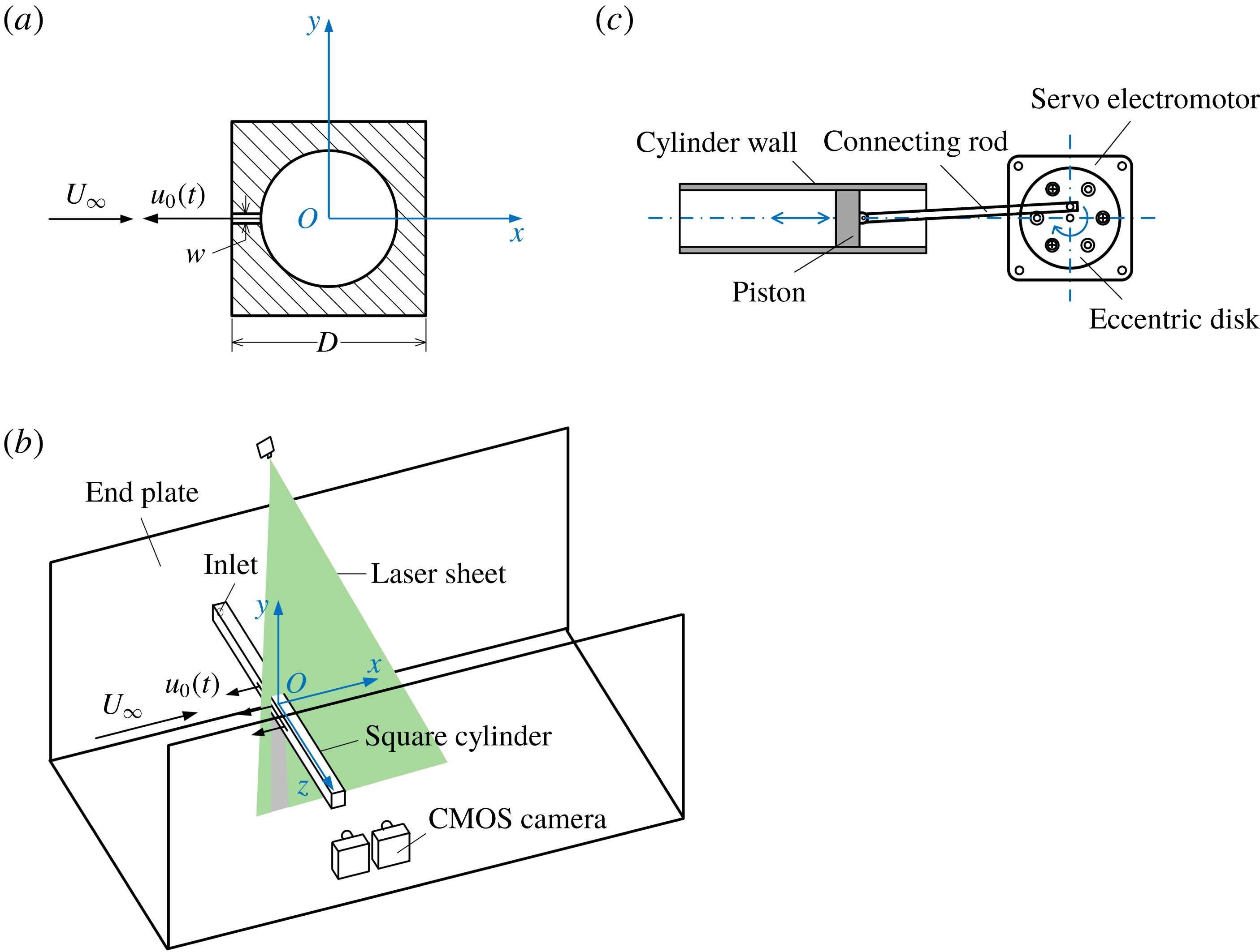
The hollow square cylinder used as the experimental model has a side width $D=20~\text{mm}$ and a span length $L_{D}=430~\text{mm}$ , and it was made of stainless steel. Figure 1(a) shows the cross-section of the square cylinder at mid-span and figure 1(b) is the sketch of the experimental arrangement. The square cylinder was fixed at the mid-height of two end plates with an incidence angle of $0^{\circ }$ , and its axis was located at $15.5D$ downstream from the leading edge. The end plates were placed parallel to the incoming flow to minimize the three-dimensional effect which is associated with the boundary layer development along the sidewalls of the water channel. The slot on the front surface of the model was designed as the synthetic jet exit, and it was positioned in the range $-2.5\leqslant z/D\leqslant 2.5$ with a width $w=1~\text{mm}$ and a length $l=100~\text{mm}$ . The cylindrical cavity with a diameter of 14 mm inside the square cylinder was connected with the slot. One end of the square cylinder was sealed, and there was an inlet at the other end.

Figure 1.

(a) Cross-section of the square cylinder at mid-span, (b) sketch of the experimental arrangement, (c) diagram of the synthetic jet actuator.

The synthetic jet excitation system is the same as the one described in our previous work (Qu et al. Reference Qu, Wang, Sun, Feng, Pan, Gao and He2017). A type of piston-driven actuator was applied to induce the synthetic jet, as demonstrated in figure 1(c). An eccentric disk was driven by a servo electromotor to rotate at a certain speed set on the computer, and the rotating speed was proportional to the excitation frequency of the synthetic jet. The eccentric disk was connected with a piston via a rod, transferring the aforementioned rotating motion to the back-and-forth movement of the piston. Between the synthetic jet actuator and the square cylinder, an ‘ $L$ ’-shaped hollow cylinder made of Plexiglass was used. Its horizontal part was directly connected to the inlet of the square cylinder and its vertical part was connected to the cylinder wall of the actuator by a rigid Teflon tube, which was not easy to deform during the excitation. The connections were checked before the experiment to ensure they had a good sealing performance. Driven by the excitation system, fluid inside the cavity of the square cylinder was forced to blow and suck through the slot in cycles, and the synthetic jet vortex pairs were thus generated at the slot exit.

2.2 Particle image velocimetry measurement

A two-dimensional time-resolved particle image velocimetry (PIV) system was set up to conduct the quantitative measurements of the flow field. In order to avoid the edge effects of the slot, the measurement was taken in the $(x,y)$ plane at the mid-span of the square cylinder. Hollow glass beads with a diameter of $5{-}20~\unicode[STIX]{x03BC}\text{m}$ and a density of $1.05~\text{g}~\text{cm}^{-3}$ were seeded in the water to accurately follow the flow. The investigation area was illuminated by a continuous laser sheet, which has a maximum output power of 8 W and emits at a wavelength of 532 nm. Under the control of a synchronizer, the particle images upstream and downstream of the square cylinder were recorded simultaneously using two identical high-speed CMOS cameras (Photron Fastcam SA2 86K-M3). The cameras use 12 bits to record colour depth and the image sensors have a full resolution of $2048\times 2048~\text{pixels}$ . Since the flow structures that these two cameras concentrated on were distributed in different areas, lenses with different focal lengths were used. For the camera upstream, the field of view (FOV) was in the range $-4\leqslant x/D\leqslant 2$ , $-2.75\leqslant y/D\leqslant 2.75$ , with a magnification of $0.06~\text{mm}~\text{pix}^{-1}$ . While for the camera downstream, the FOV was in the area of $-1\leqslant x/D\leqslant 11$ , $-5.75\leqslant y/D\leqslant 5.75$ , with a magnification of $0.12~\text{mm}~\text{pix}^{-1}$ . 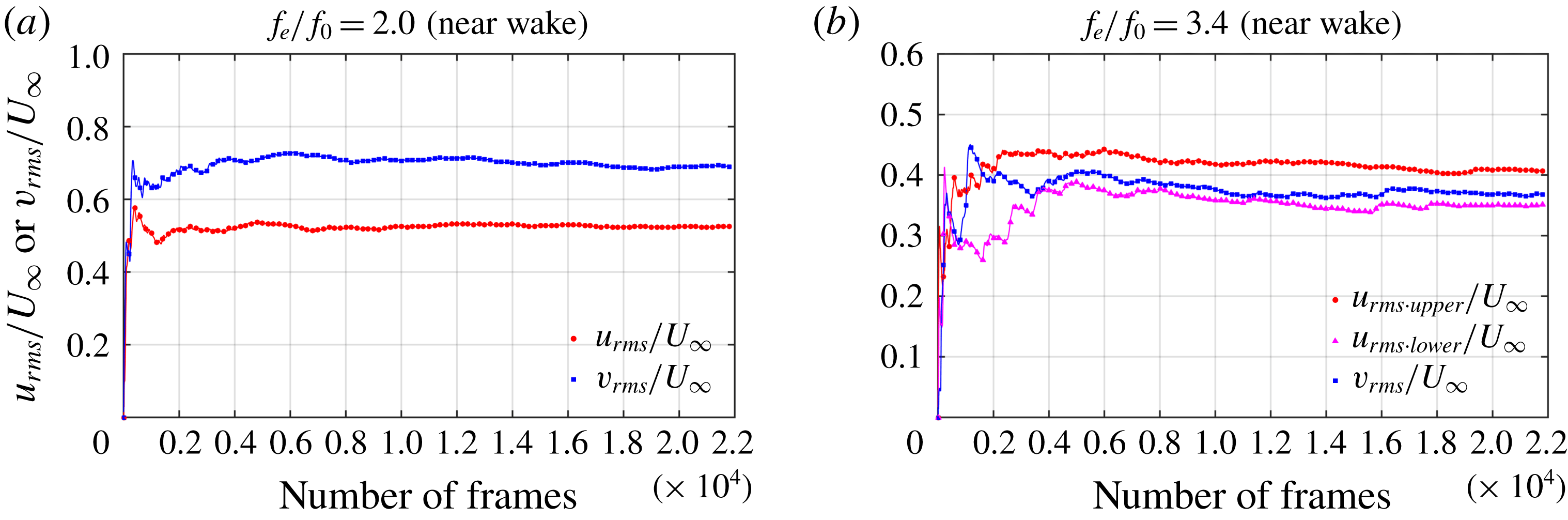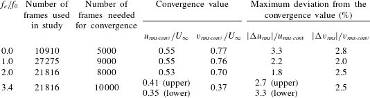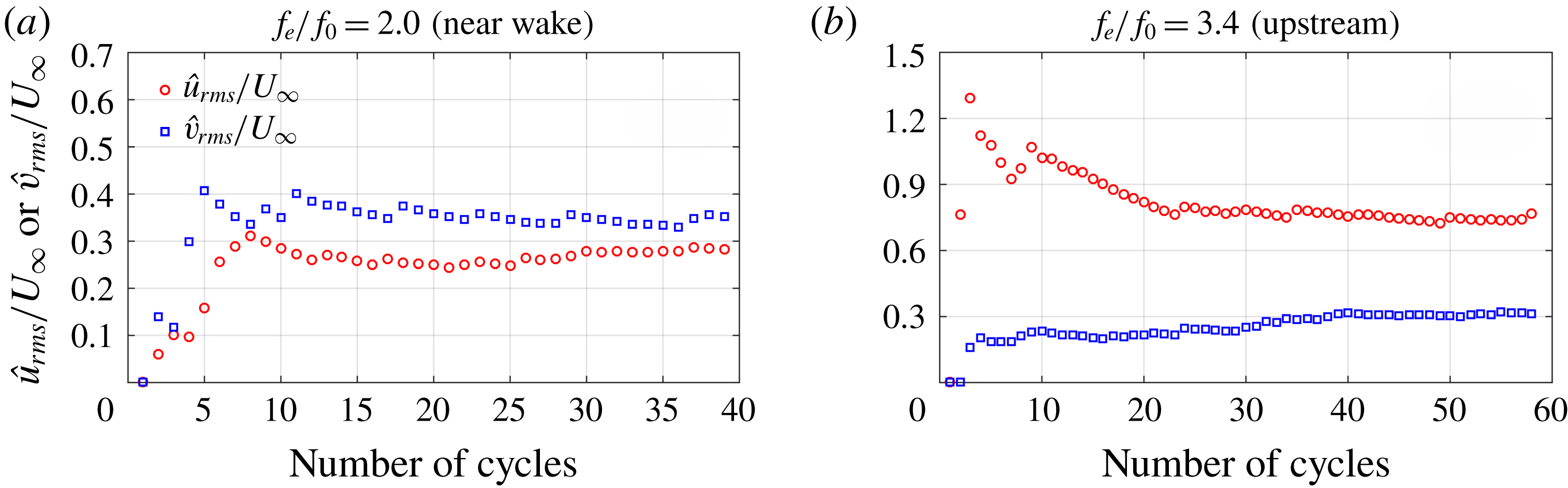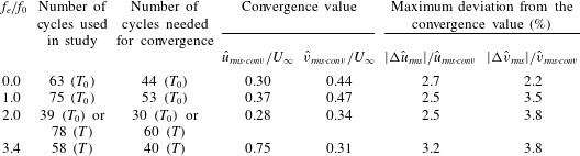The sampling rate was selected from 50 Hz to 150 Hz with the increase of the synthetic jet exit velocity. The exposure time was no longer than 3.3 ms to guarantee good image quality. Limited by the storage capacity of the cameras, a repetition of 5457 frames could be continuously captured at a time for each camera under the current spatial resolution. In the present investigation, at least 10 910 snapshots are used to calculate the time-averaged statistics. For the natural case, 63 wake vortex-shedding cycles are used during the calculation of phase averaging, while at least 58 excitation cycles are employed to calculate the phase-averaged quantities for the control cases. The convergence test has verified that the sample sizes used are sufficient for the convergence of the root-mean-square (r.m.s.) of velocity fluctuations in the time-averaged and phase-averaged flow fields. More details about the statistical convergence of parameters are provided in appendix A.

The multi-pass iterative Lucas–Kanade algorithm (known as MILK) was used to calculate the velocity vector fields from the PIV images. This algorithm has a high computation efficiency by using graphic processing units (known as GPU) parallelization and can output a dense velocity field up to pixel-level (Champagnat et al. Reference Champagnat, Plyer, le Besnerais, Leclaire, Davoust and le Sant2011; Pan et al. Reference Pan, Xue, Xu, Wang and Wei2015). A final interrogation window of $32\times 32$ pixels with a 75 % overlap was used for both the images upstream and downstream.

2.3 Experimental parameters

During the experiment, the free-stream velocity was kept constant at $U_{\infty }=43~\text{mm}~\text{s}^{-1}$ . The water temperature was around $27\,^{\circ }\text{C}$ , and the corresponding kinematic viscosity coefficient was $\unicode[STIX]{x1D708}=0.854\times 10^{-6}~\text{m}^{2}~\text{s}^{-1}$ . The Reynolds number based on the free-stream velocity $U_{\infty }$ and the side width $D$ of the square cylinder was $Re_{D}=U_{\infty }D/\unicode[STIX]{x1D708}=1000$ . It is necessary to point out here that the wake flow is conjectured to be three-dimensional at current $Re_{D}$ . As proposed in Sohankar, Norberg & Davidson (Reference Sohankar, Norberg and Davidson1999) and Jiang, Cheng & An (Reference Jiang, Cheng and An2018), three-dimensional wake transition occurs for flow past a square cylinder when the Reynolds number is beyond the critical value $Re_{cr}$ . The value of $Re_{cr}$ varies slightly in different studies and is 165.7 in Jiang et al. (Reference Jiang, Cheng and An2018). The three-dimensionality of flow continuously increases with $Re$ since the onset of wake transition (Jiang et al. Reference Jiang, Cheng and An2018). At $Re=1000$ , vortex dislocations and wavy deformations of spanwise vorticity were observed by Lou et al. (Reference Lou, Zhou, Jiang and Cheng2016), and a three-dimensional topology concerning Kelvin–Helmholtz vortices, von Kármán vortex street and streamwise vortex structures was described by Brun & Goossens (Reference Brun and Goossens2008) in the square cylinder wake. Nevertheless, the present study is mainly concentrated on the statistical characteristics in the wake (the phase-averaged wake structures and time-averaged quantities, as will be shown in § 3). The PIV measurement was only conducted in the $(x,y)$ plane at the mid-span of the square cylinder, and the variation of instantaneous wake structure along the span is beyond the scope of our discussion. Feng, Ma & Wang (Reference Feng, Ma and Wang2014) has proved that the statistics presented good consistency in the planes near the mid-span in their experiment using the synthetic jet to control the flow around a circular cylinder. Both the aspect ratio of the cylinder and the ratio of the slot length to the cylinder diameter in our experiment are larger than those in Feng et al. (Reference Feng, Ma and Wang2014). From the perspective of statistics, the two-dimensional characteristic near the mid-span regions in the near wake could be conjectured as acceptable.

The wake vortex-shedding frequency $f_{0}$ is 0.29 Hz for the natural case under current experimental conditions. This value is obtained through the frequency spectrum analysis of the streamwise velocity history at the point where the r.m.s. of the streamwise velocity fluctuation is maximal in the shear layer. The Strouhal number is 0.136, given by $St=f_{0}D/U_{\infty }$ . As the variable in the present study, the dimensionless excitation frequency, defined as the excitation frequency $f_{e}$ normalized by the natural wake vortex-shedding frequency $f_{0}$ , was set at different values of $f_{e}/f_{0}=0$ , 0.6, 1.0, 2.0 and 3.4. As mentioned in § 2.1, the excitation frequency can be changed by adjusting the rotating speed of the servo electromotor in figure 1(c). Since the unit of the rotating speed is revolutions per minute (r.p.m.) and the value can only be set at an integer in the current system, the speeds corresponding to the above excitation frequencies were 0, 10, 18, 35 and 59 r.p.m.

According to Smith & Glezer (Reference Smith and Glezer1998), there are two important dimensionless parameters to characterize the synthetic jet: the synthetic jet Reynolds number and the dimensionless stroke length. The synthetic jet Reynolds number is based on the synthetic jet exit velocity. Let $u_{0}(t)$ denote the instantaneous streamwise velocity at the slot exit. Since the working fluid can be considered incompressible and the synthetic jet has acceptable two-dimensional characteristic along the exit, driven by the synthetic jet actuator, the $u_{0}(t)$ can be described by the following sine function

(2.1) $$\begin{eqnarray}u_{0}(t)=\frac{\unicode[STIX]{x03C0}^{2}D_{P}^{2}}{2lw}Af_{e}\sin (2\unicode[STIX]{x03C0}f_{e}t).\end{eqnarray}$$

Here, the symbol $t$ denotes time; $A=3.3~\text{mm}$ is the offset distance of the eccentric disk; $D_{P}=29~\text{mm}$ is the outer diameter of the piston encased in the cylinder wall; symbols $l$ and $w$ are the length and width of the slot, respectively. The dimensionless stroke length, which is the stroke length $L_{0}$ normalized by the slot width $w$ , can be expressed by

(2.2) $$\begin{eqnarray}L_{0}/w=\frac{1}{w}\int _{0}^{T/2}u_{0}(t)\,\text{d}t=\frac{\unicode[STIX]{x03C0}AD_{P}^{2}}{2lw^{2}},\end{eqnarray}$$

where $T=1/f_{e}$ is the excitation period. It can be seen that the dimensionless stroke length is independent of the excitation frequency and is thus fixed at $L_{0}/w=43.6$ in the investigation. The time-averaged blowing velocity over an excitation cycle is represented by $\overline{U_{0}}$ , and can be calculated from

(2.3) $$\begin{eqnarray}\overline{U_{0}}=L_{0}/T=\frac{1}{T}\int _{0}^{T/2}u_{0}(t)\,\text{d}t=\frac{\unicode[STIX]{x03C0}AD_{P}^{2}f_{e}}{2lw}.\end{eqnarray}$$

Finally, the synthetic jet Reynolds number $Re_{\overline{U_{0}}}$ , which is based on $\overline{U_{0}}$ and the slot width $w$ , is defined as

(2.4) $$\begin{eqnarray}Re_{\overline{U_{0}}}=\frac{\overline{U_{0}}w}{\unicode[STIX]{x1D708}}=\frac{\unicode[STIX]{x03C0}AD_{P}^{2}f_{e}}{2l\unicode[STIX]{x1D708}}.\end{eqnarray}$$

Hence, the values of $\overline{U_{0}}$ corresponding to the above excitation frequencies are $\overline{U_{0}}=0$ , 7.3, 13.1, 25.4 and $42.9~\text{mm}~\text{s}^{-1}$ , and further, the synthetic jet Reynolds numbers are $Re_{\overline{U_{0}}}=0$ , 9, 15, 30 and 50. The definitions of parameters associated with the synthetic jet in above equations make reference to the previous works (Smith & Glezer Reference Smith and Glezer1998; Amitay & Cannelle Reference Amitay and Cannelle2006; Feng & Wang Reference Feng and Wang2010; Qu et al. Reference Qu, Wang, Sun, Feng, Pan, Gao and He2017).

2.4 Uncertainty analysis

The uncertainties of velocity measured by PIV and some quantities derived from velocity are evaluated in this section.

2.4.1 Uncertainty of instantaneous velocity

The particle velocity $u_{p}$ in the PIV measurement can be expressed by

(2.5) $$\begin{eqnarray}u_{p}=x_{p}/t_{p},\end{eqnarray}$$

here $x_{p}$ is the particle displacement between adjacent frames and $t_{p}$ is one sampling interval. The uncertainty of $u_{p}$ comes from both the uncertainties of $x_{p}$ and $t_{p}$ , and can be estimated by the uncertainty propagation formula (Kline & McClintock Reference Kline and McClintock1953), thus

(2.6) $$\begin{eqnarray}\unicode[STIX]{x1D700}(u_{P})=\sqrt{\left(\frac{\unicode[STIX]{x2202}u_{P}}{\unicode[STIX]{x2202}x_{P}}\right)^{2}\unicode[STIX]{x1D700}^{2}(x_{P})+\left(\frac{\unicode[STIX]{x2202}u_{P}}{\unicode[STIX]{x2202}t_{P}}\right)^{2}\unicode[STIX]{x1D700}^{2}(t_{P})}=\sqrt{\left(\frac{1}{t_{p}}\right)^{2}\unicode[STIX]{x1D700}^{2}(x_{P})+\left(-\frac{x_{P}}{t_{P}^{2}}\right)^{2}\unicode[STIX]{x1D700}^{2}(t_{P})},\end{eqnarray}$$

where $\unicode[STIX]{x1D700}$ denotes the uncertainty. Since $\unicode[STIX]{x1D700}(t_{P})$ is really small, the item containing $\unicode[STIX]{x1D700}(t_{P})$ is negligible. The maximum absolute uncertainty of $x_{p}$ is 0.1 pixel according to He et al. (Reference He, Pan, Feng, Gao and Wang2016) and Raffel et al. (Reference Raffel, Willert, Scarano, Kähler, Wereley and Kompenhans2018). With the highest sampling rate of 150 Hz and current image magnifications mentioned in § 2.2, the absolute uncertainties of velocity $\unicode[STIX]{x1D700}(U)$ computed based on (2.6) are less than $0.9~\text{mm}~\text{s}^{-1}$ and $1.8~\text{mm}~\text{s}^{-1}$ for the upstream and downstream flow fields, respectively. The relative uncertainties are no more than 0.9 % and 1.7 % for the two fields, calculated by the absolute velocity uncertainty of each case relative to the respective maximum velocity in the flow.

2.4.2 Uncertainty of vorticity

The spanwise vorticity $\unicode[STIX]{x1D714}_{z}$ is calculated from the velocity field by the central-difference scheme,

(2.7) $$\begin{eqnarray}\unicode[STIX]{x1D714}_{z}(x,y)=\frac{1}{2s}[v(x+s,y)-v(x-s,y)-(u(x,y+s)-u(x,y-s))],\end{eqnarray}$$

where $s$ is the space interval between two adjacent velocity vectors. The values of $s$ are 0.48 mm and 0.96 mm, respectively, for the present upstream and downstream velocity fields. The uncertainties of the streamwise velocity and the vertical velocity are the same $(\unicode[STIX]{x1D700}(u)=\unicode[STIX]{x1D700}(v)=\unicode[STIX]{x1D700}(U))$ . According to Sciacchitano & Wieneke (Reference Sciacchitano and Wieneke2016), the uncertainty of vorticity has the form of

(2.8) $$\begin{eqnarray}\unicode[STIX]{x1D700}(\unicode[STIX]{x1D714}_{z})=\frac{\unicode[STIX]{x1D700}(U)}{s}\sqrt{1-r(2s)},\end{eqnarray}$$

here $r(2s)$ is the cross-correlation coefficient between two vectors with a space interval $2s$ , and its value is approximately 0.45 with current interrogation window of $32\times 32$ pixels and overlap of 75 %, computed via a Monte Carlo simulation by Sciacchitano & Wieneke (Reference Sciacchitano and Wieneke2016). Hence, the uncertainty of vorticity is computed to be less than $1.39~\text{s}^{-1}$ in the whole flow fields, i.e. equal to 0.65 normalized by the free-stream velocity $U_{\infty }$ and the side length $D$ of the square cylinder.

2.4.3 Uncertainty of time-averaged velocity and velocity fluctuation

Following Sciacchitano & Wieneke (Reference Sciacchitano and Wieneke2016), the uncertainty of the time-averaged streamwise velocity $\overline{U}$ is derived from

(2.9) $$\begin{eqnarray}\unicode[STIX]{x1D700}(\overline{U})=\frac{\unicode[STIX]{x1D70E}(u)}{\sqrt{N}},\end{eqnarray}$$

where $N$ is the sample size over time and $\unicode[STIX]{x1D70E}(u)$ is the standard deviation of the streamwise velocity. The value of $\unicode[STIX]{x1D70E}(u)$ should actually consist of two parts: the true velocity fluctuations and the measurement errors. Because the latter are much smaller than the former, the measurement errors in $\unicode[STIX]{x1D70E}(u)$ are ignored here. By substituting the value of $N$ and the maximum $\unicode[STIX]{x1D70E}(u)$ in the flow for each individual case, the uncertainty of $\overline{U}$ is expected to be less than $0.53\,\%U_{\infty }$ .

Similarly, a maximum uncertainty of 0.37 % relative to $U_{\infty }$ is obtained for the root-mean-square of the streamwise velocity fluctuation $u_{rms}$ , estimated as

(2.10) $$\begin{eqnarray}\unicode[STIX]{x1D700}(u_{rms})\approx \unicode[STIX]{x1D700}(\unicode[STIX]{x1D70E}(u))=\frac{\unicode[STIX]{x1D70E}(u)}{\sqrt{2(N-1)}}.\end{eqnarray}$$

Likewise, the uncertainty of $v_{rms}$ is no more than $0.52\,\%U_{\infty }$ . It should be noted that the uncertainties of the time-averaged velocity and velocity fluctuations assessed above might be underestimated due to the absence of some random and systematic errors (Sciacchitano & Wieneke Reference Sciacchitano and Wieneke2016).

3.1 Evolution of vortex structures

Proper orthogonal decomposition is a statistical tool to extract the dominant features from the complicated flow field in experiments or simulations (Berkooz, Holmes & Lumley Reference Berkooz, Holmes and Lumley1993; Weightman et al. Reference Weightman, Amili, Honnery, Soria and Edgington-Mitchell2018). The POD can be described mathematically by the following expression:

(3.1) $$\begin{eqnarray}\boldsymbol{u}^{\prime }(\boldsymbol{x},t)\approx \mathop{\sum }_{i=1}^{K}a_{i}(t)\unicode[STIX]{x1D753}_{i}(\boldsymbol{x}),\end{eqnarray}$$

where $\boldsymbol{x}$ denotes spatial coordinate; $\boldsymbol{u}^{\prime }(\boldsymbol{x},t)$ is the spatiotemporal fluctuation velocity field; $\unicode[STIX]{x1D753}_{i}(\boldsymbol{x})$ is the $i$ th mode with the spatial characteristics; $a_{i}(t)$ is the time coefficient corresponding to the $i$ th mode, and $K$ is the total number of modes decomposed. It can be seen that POD is a linear procedure. The purpose of this method is actually to find an optimal low-dimensional approximation of the high-dimensional system. The modes are ranked in descending order of energy (Sirovich Reference Sirovich1987; Berkooz et al. Reference Berkooz, Holmes and Lumley1993; Chatterjee Reference Chatterjee2000; Zhang, Liu & Wang Reference Zhang, Liu and Wang2014; Deng et al. Reference Deng, Pan, Wang and Rinoshika2017). For flow over a bluff body, it has been proved that the first two POD modes, which are closely related to the von Kármán vortex street (Ma, Karamanos & Karniadakis Reference Ma, Karamanos and Karniadakis2000; Perrin et al. Reference Perrin, Braza, Cid, Cazin, Moradei, Barthet, Sevrain and Hoarau2006, Reference Perrin, Braza, Cid, Cazin, Barthet, Sevrain, Mockett and Thiele2007), make a dominant contribution to the total energy, e.g. nearly 70 % for flow over a square cylinder (van Oudheusden et al. Reference van Oudheusden, Scarano, van Hinsberg and Watt2005; Qu et al. Reference Qu, Wang, Sun, Feng, Pan, Gao and He2017). The time coefficients of the first two POD modes, which tend to distribute around a circle in the normalized $(a_{1},a_{2})$ plane, are thus used as the phase indicator for the quasi-periodic flow in our present study. The details about this algorithm can be found in van Oudheusden et al. (Reference van Oudheusden, Scarano, van Hinsberg and Watt2005) and Pan, Wang & Wang (Reference Pan, Wang and Wang2013). The $\unicode[STIX]{x1D706}_{ci}$ method is used as a criterion to visualize vortices. According to Zhou et al. (Reference Zhou, Adrian, Balachandar and Kendall1999), the imaginary part of the complex eigenvalue pair of the velocity gradient tensor is denoted as $\unicode[STIX]{x1D706}_{ci}$ , and it is regarded as the local swirling strength of the vortex. With this method, the evolution of vortices can be clearly demonstrated.

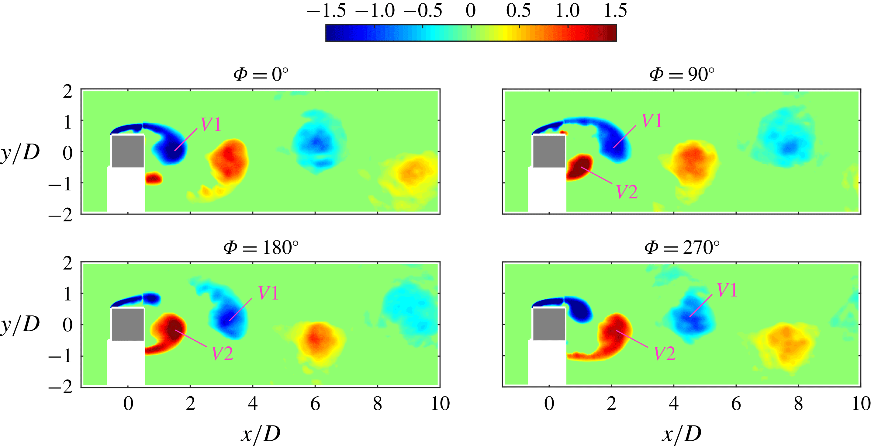
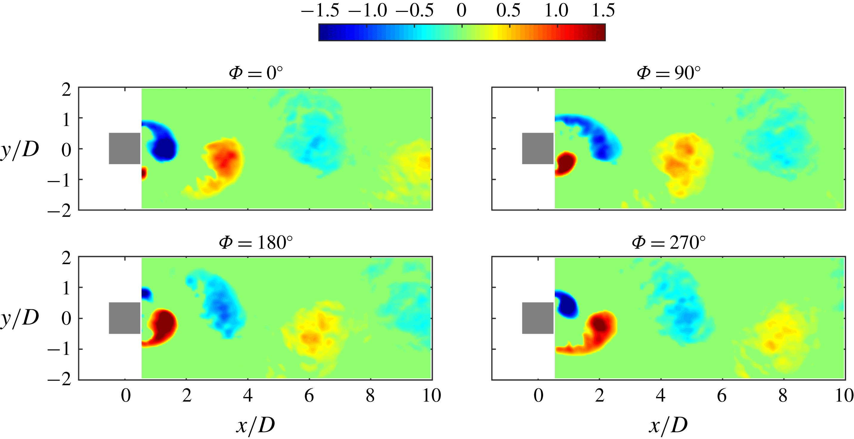
Figure 2 shows the phase-averaged $\unicode[STIX]{x1D706}_{ci}$ field for the natural case. The sign of $\unicode[STIX]{x1D706}_{ci}$ is the same as the local vorticity. Because the whole flow field is obtained by splicing the upstream and downstream flow fields together, a seam line can be observed at the location of approximately $x/D=10$ , however, it has little effect on the current analysis. The familiar von Kármán vortex-shedding process is presented in figure 2. Flow separates at the front corners of the square cylinder and forms shear layers around the side surfaces. The shear layer on the upper side rolls up into a vortex $V1$ in the wake $(\unicode[STIX]{x1D6F7}=0^{\circ })$ . The vortex $V1$ grows gradually by entraining the surrounding fluid, at the same time, the fluid on the lower side tends to be drawn across the wake by the entrainment effect and it carries the vorticity of the opposite sign $(\unicode[STIX]{x1D6F7}=90^{\circ })$ . When the circulation accumulates to a certain extent, vortex $V1$ sheds off from the upper shear layer and convects downstream. Vortex $V2$ on the lower side has rolled up at the moment and finally separates from the lower shear layer after a similar process. For the natural case, the alternative vortex shedding in the wake is the 2S mode (Williamson & Roshko Reference Williamson and Roshko1988).

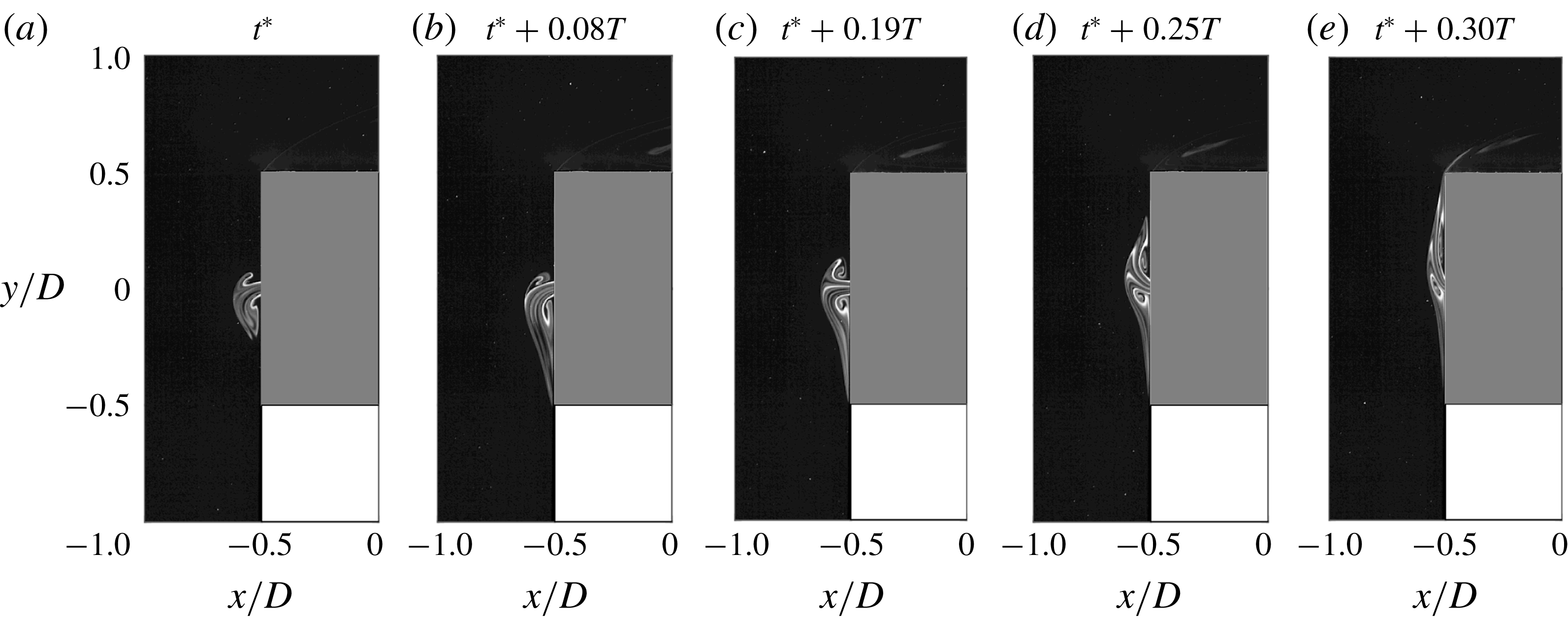
The laser-induced fluorescence (LIF) technique was used to visualize the flow structures qualitatively. The fluorescent dye rhodamine B was added into the inner cavity of the square cylinder so that it could be blown out together with the synthetic jet. The evolution of the flow structures around the front surface of the square cylinder for $f_{e}/f_{0}=0.6$ is shown in figure 3. In the initial stage of the blowing stroke, the injected flow separates at the edges of the slot, generating a pair of counter-rotating synthetic jet vortices. At time $t^{\ast }$ (figure 3 a), the synthetic jet vortex pair is not symmetric about the $y$ -axis but inclines toward the $-y$ direction. The lower synthetic jet vortex is observed to be a little larger than the upper one at this moment. The vortex pair then moves downward, and the lower part is stretched successively, covering a longer distance in the $-y$ direction, as shown in figure 3(b). After that, the vortices change their moving direction and shift upward. The vortex structures become more and more symmetric. At $t^{\ast }+0.19T$ (figure 3 c), the two vortices are of similar size, and the shear layer between them is nearly straight along the $y$ -axis. Whereafter, the synthetic jet continues to deflect toward the $+y$ direction, and the vortex pair becomes longer and narrower in shape as a result of the stretch in the vertical direction (figure 3 d). Finally, they pass around the upper front corner of the square cylinder and are drawn into the upper shear layer. The vortices are always attached to the front surface of the square cylinder in this case. Note that the strength of the synthetic jet is really weak in this case, the wake vortices remain largely unaffected.

Figure 2.

Phase-averaged $\unicode[STIX]{x1D706}_{ci}D/U_{\infty }$ field within a wake vortex-shedding cycle for the natural case.

Figure 3.

Flow visualization of the instantaneous flow structures near the front surface of the square cylinder for $f_{e}/f_{0}=0.6$ . The initial time $t^{\ast }$ is arbitrary. Here $T$ is one excitation period of the synthetic jet.

In the study of Huang et al. (Reference Huang, Hsu and Chiu2014), where a planar jet was injected from the front surface of a square cylinder, a recirculation bubble containing two counter-rotating vortices was also observed on the front surface in the range $R<1$ . Induced by the periodic wake vortex shedding, this vortex pair swung periodically with time. However, in the present case with the control of the synthetic jet, whether the vortex pair firstly deflects toward the $-y$ or $+y$ direction for each excitation cycle is not certain. The reasons for this difference are discussed as follows: for a square cylinder without control, Huang et al. (Reference Huang, Hsu and Chiu2014) proved that the alternative vortex shedding in the wake could influence the boundary layers near the side surfaces, and further change the flow characteristics around the front surface. They found that the front stagnation point of a square cylinder is not fixed at the central point of the front surface but oscillates periodically in the range $-0.08\leqslant y/D\leqslant 0.08$ . For the current experimental model, the slot as the synthetic jet exit is located at $-0.025\leqslant y/D\leqslant 0.025$ , within the oscillating range of the stagnation point. As the synthetic jet has a small momentum in this case, the instability of the synthetic jet is too weak to take over the dominant role of the inherent instability. Thus, the synthetic jet is under the influence of the upstream propagating signal from the wake. Unlike the continuous jet, which is a steady blowing, the synthetic jet has its own excitation period which is not synchronous with the period of wake vortex shedding. Every time the synthetic jet starts the blowing stroke, the flow conditions around the slot may be at different phases, and thus the initial deflecting direction of the synthetic jet vortex pair is not certain for each excitation cycle. It can be inferred that a four-way saddle exists in the vicinity of the front surface during the blowing cycle of the excitation, due to the impingement between the free stream and the synthetic jet. This kind of saddle was also observed when the swinging jet mode appeared for a square cylinder with a front jet injection (Hsu et al. Reference Hsu, Huang and Chung2016) and when a closed envelope formed for a circular cylinder with a slot synthetic jet injecting toward upstream (Wang et al. Reference Wang, Feng and Xu2007).

Figure 4.

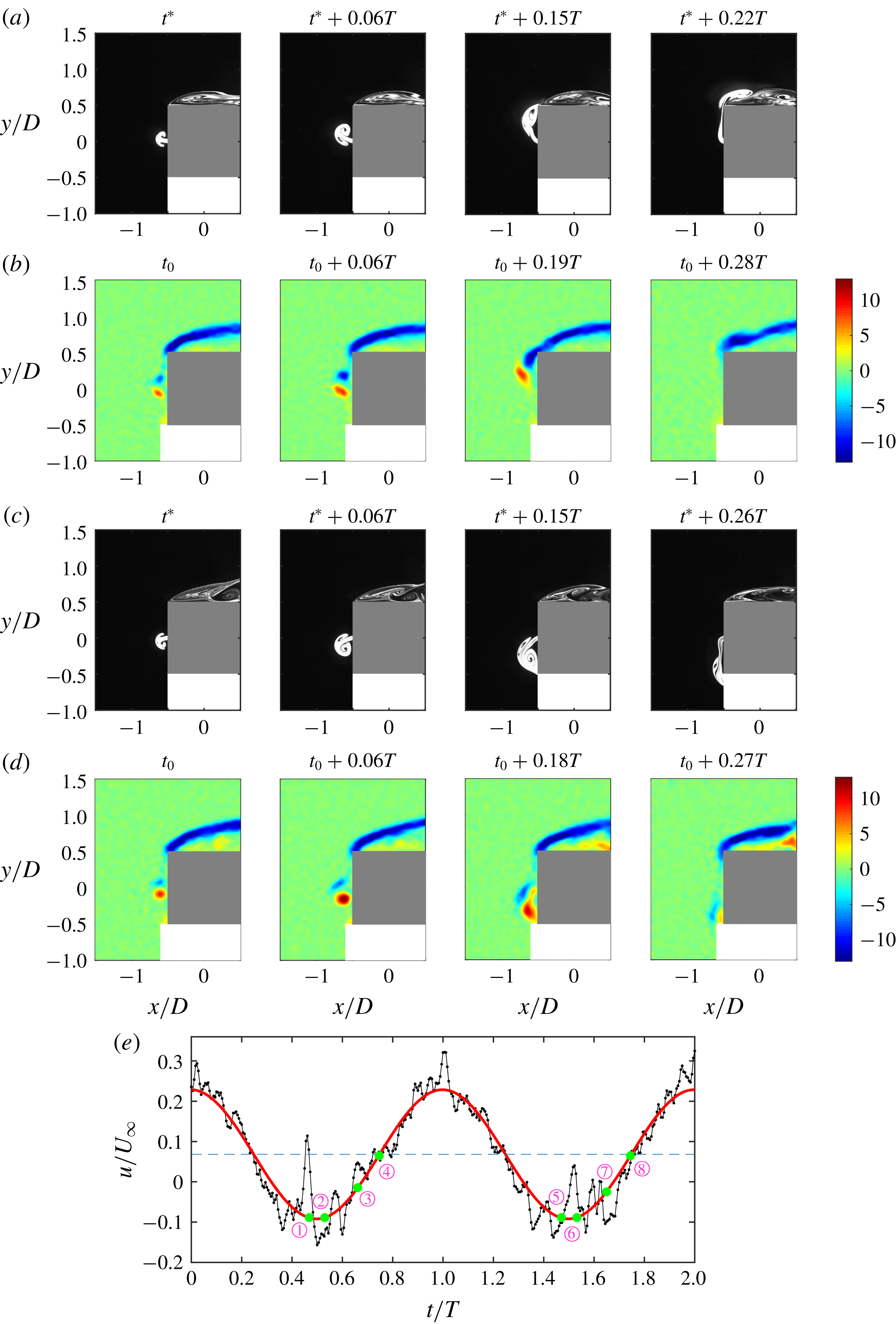
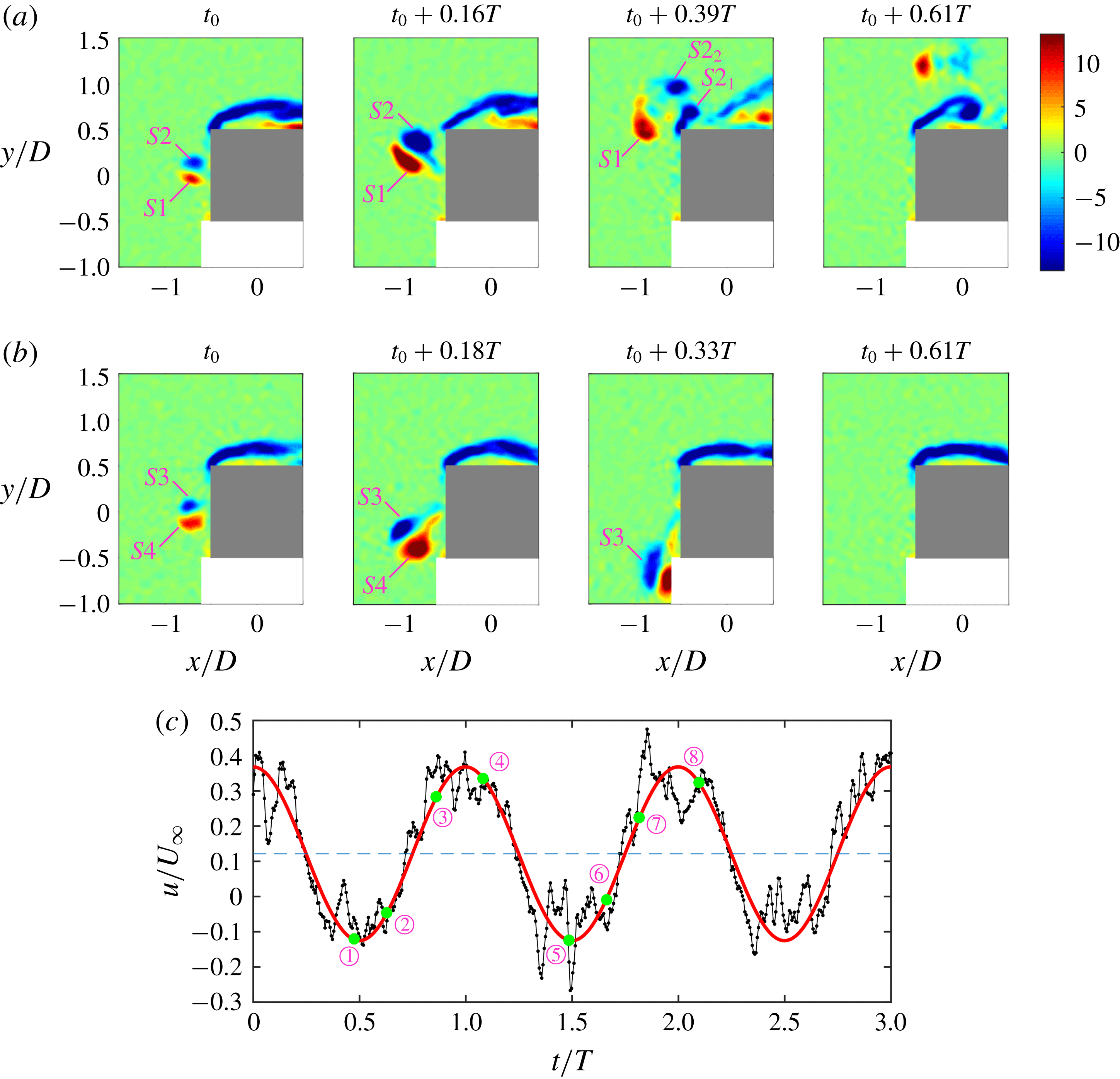
Evolution of the instantaneous flow structures upstream of the rear surface of the square cylinder for $f_{e}/f_{0}=1.0$ . The initial time $t^{\ast }$ and $t_{0}$ are arbitrary. Here $T$ is one excitation period of the synthetic jet. (a,c) Flow visualization results obtained by LIF, (b,d) instantaneous spanwise vorticity $\unicode[STIX]{x1D714}_{z}D/U_{\infty }$ obtained by PIV, (e) streamwise velocity history (in black) and the fitting sine function (in red) at $(x/D,y/D)=(-0.55,0)$ measured by PIV.

The synthetic jet vortices develop differently when $f_{e}/f_{0}$ is increased to 1.0. Figure 4 presents the instantaneous flow structures upstream of the square cylinder obtained by the qualitative visualization of LIF and the quantitative measurement of PIV. As a result of the quasi-periodic flow characteristic, there is a slight time shift between the corresponding patterns captured with these two methods. Due to the limited spatial resolution of PIV, the pixel distance corresponding to the width of the synthetic jet exit is smaller than the side length of the interrogation window in the velocity calculation, and thus the synthetic jet velocity at the slot cannot be measured precisely. Instead, the streamwise velocity history at $(x/D,y/D)=(-0.55,0)$ is provided in figure 4(e) in black. On the one hand, this point is more than half of the side length of the interrogation window away from the wall, and thus the influence of the wall on the calculation of velocity field can be avoided. On the other hand, the velocity at this point has a good periodicity, with its peak frequency identical to the excitation frequency of the synthetic jet. Since the instantaneous streamwise velocity at the slot exit is a sine function in theory (2.1), the streamwise velocity at the selected point is also fitted with a sine function, as shown in red. Note that there might be a magnitude difference and a phase difference between the velocity at $(x/D,y/D)=(-0.55,0)$ and that at the synthetic jet exit, however, it is reasonable and helpful to use the former as a reference in order to reveal the evolution of flow structures with the actuation of the synthetic jet. The points $\unicode[STIX]{x2460}$ to $\unicode[STIX]{x2463}$ , respectively, correspond to the four instants in figure 4(b), and the points $\unicode[STIX]{x2464}$ to $\unicode[STIX]{x2467}$ correspond to those in figure 4(d). Within one excitation cycle, the synthetic jet vortex pair only deflects toward one side, i.e. either the $+y$ direction or the $-y$ direction (hereinafter referred to as the upward deflection condition and the downward deflection condition), and does not turn to the other side. The deflecting direction is still not predictable. Statistically, among the 152 excitation cycles recorded by PIV, the number of cycles in the upward deflection condition is quite close to that in the downward deflection condition. Take the upward deflection condition as an example to briefly describe the vortex evolution process; at $t_{0}$ in figure 4(b), a counter-rotating synthetic jet vortex pair has already generated near the slot. The synthetic jet started its blowing cycle before this moment, thus the streamwise velocity in figure 4(e) continuously decreases to the negative value at point $\unicode[STIX]{x2460}$ , which is close to the minimum. From $t_{0}$ to some point after $t_{0}+0.06T$ , the synthetic jet vortices grow gradually as they deflect upward. Compared with the case of $f_{e}/f_{0}=0.6$ , the vortices are larger in size and stronger in strength, and they are not always attached to the front surface of the square cylinder due to a higher momentum. Influenced by the deflection, the lower synthetic jet vortex is slim while the upper one has a plumper shape, as shown at time $t^{\ast }+0.06T$ in figure 4(a). The synthetic jet vortices constantly deform and the upper vortex contacts with the upper front corner of the square cylinder ( $t_{0}+0.19T$ in figure 4 b and $t^{\ast }+0.15T$ in figure 4 a). Later, the patterns flow into the region near the top surface of the square cylinder and interact with the upper shear layer ( $t_{0}+0.28T$ in figure 4 b and $t^{\ast }+0.22T$ in figure 4 a). It can be seen that the streamwise velocity in figure 4(e) continuously increases from $t_{0}+0.06T$ (point $\unicode[STIX]{x2461}$ ) to $t_{0}+0.28T$ (point $\unicode[STIX]{x2463}$ ). This can be attributed to the attenuation of the synthetic jet blowing velocity on the one hand and the decrease of the streamwise velocity component caused by the vortex deflection on the other hand. Influenced by the suction cycle of the synthetic jet, the streamwise velocity at the selected point later undergoes a first increasing and then decreasing trend. The evolution of synthetic jet vortices in the downward deflection condition in figure 4(c,d) with the corresponding streamwise velocity variation in figure 4(e) is similar to that in the upward deflection condition, except that the deflecting direction is opposite. From the phase-averaged $\unicode[STIX]{x1D706}_{ci}$ field in figure 5, it can be seen that the wake vortices still keep the 2S shedding mode for $f_{e}/f_{0}=1.0$ . The wake vortices seem to dissipate more quickly in the downstream compared with those in the natural case in figure 2. The continuous jet was also found to deflect to either side in the range $1<R<4.3$ by Huang et al. (Reference Huang, Hsu and Chiu2014). The deflecting direction was similarly not certain, and this is attributed to the Coandă effect. Instead of a vortex pair, a fluid bubble, where three vortices were wrapped, formed on the deflected side of the cylinder’s front surface. The wake vortex-shedding mode was also not changed by the continuous jet in this state.

The development of vortices for $f_{e}/f_{0}=2.0$ is distinct from the former cases. The synthetic jet vortex pair deflects upward and downward alternately and periodically. The shedding period of wake vortices is double of the excitation period of synthetic jet, which will be further discussed in the later section of power spectrum analysis. Figure 6 shows the evolution of instantaneous flow structures around the front surface of the square cylinder with the streamwise velocity history at $(x/D,y/D)=(-0.55,0)$ . As the instantaneous velocity varies during the blowing cycle, the evolution of the synthetic jet vortices $S1$ and $S2$ shows some similarity with that in figure 4. For example, the vortices have already generated at point $\unicode[STIX]{x2460}$ which is near the minimum instantaneous streamwise velocity, and grow and deflect between points $\unicode[STIX]{x2460}$ and $\unicode[STIX]{x2461}$ . Nevertheless, the vortex pair in this case is much stronger, and the vortex $S2$ has been divided into two parts $S2_{1}$ and $S2_{2}$ at point $\unicode[STIX]{x2462}$ , after contacting with the upper front corner of the square cylinder.

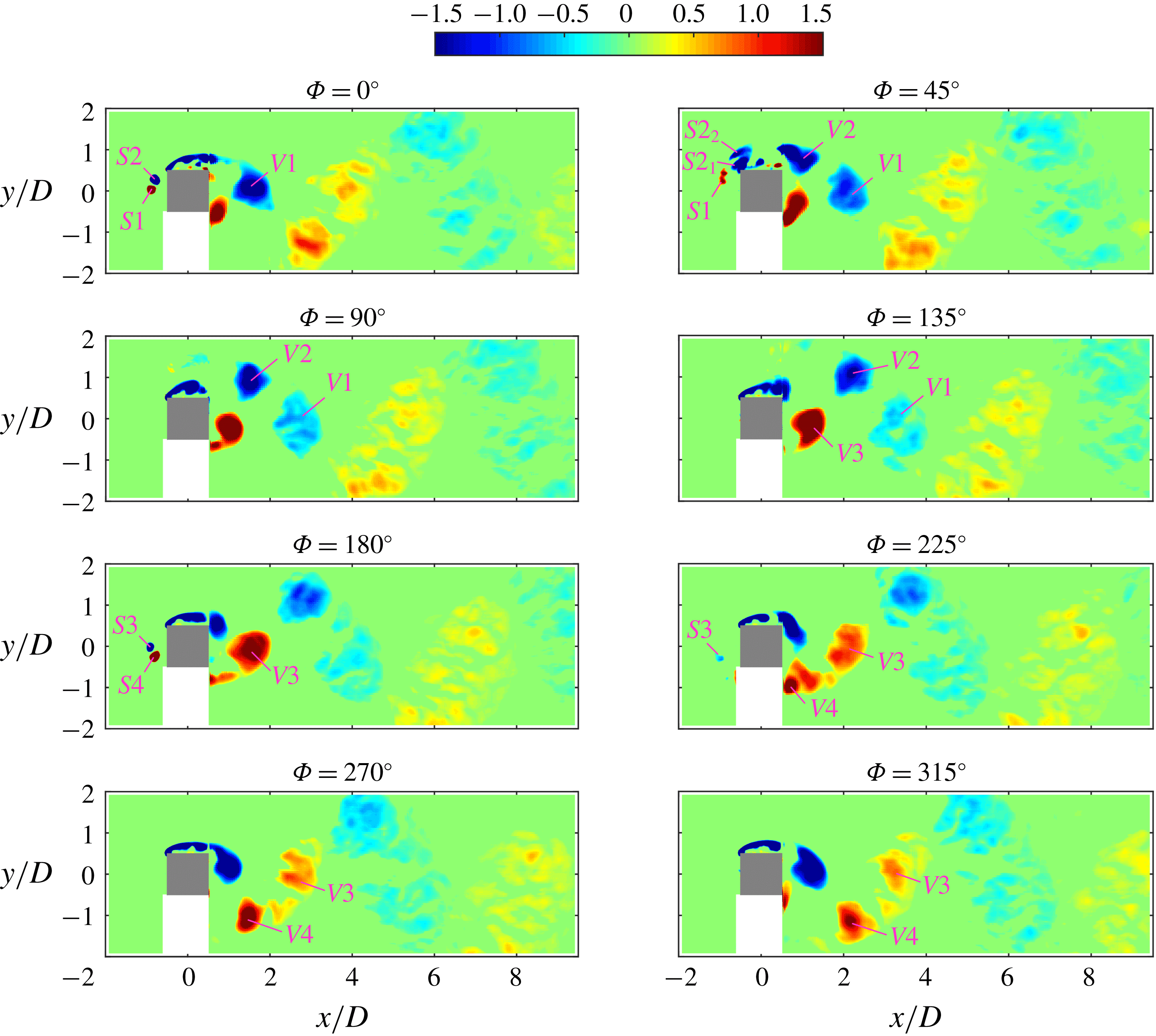
The phase-averaged $\unicode[STIX]{x1D706}_{ci}$ field within one wake vortex-shedding cycle for $f_{e}/f_{0}=2.0$ is demonstrated in figure 7, illustrating both the evolution of the synthetic jet vortices and the wake vortices. The following phase-averaging method is used rather than the one based on the first two POD coefficients: the fitting curve of the streamwise velocity at the point $(x/D,y/D)=(-0.55,0)$ is chosen as the reference signal to determine the phase. As the excitation period and the sampling frequency for a certain case are constant, the number of frames captured per excitation period is nearly the same. Thus, the whole sample can be divided into several parts, and each part covers one excitation cycle. The phases of the frames in each part can be easily identified according to their order in the time scale. The phase averaging is conducted based on this method of phase identification. The synthetic jet vortices deflect upward during the first excitation cycle (i.e. the first half of the wake vortex-shedding cycle). As shown at $\unicode[STIX]{x1D6F7}=0^{\circ }$ , the lower part of the synthetic jet vortex pair $S1$ has positive vorticity and the upper one $S2$ has negative vorticity. At this time, a wake vortex $V1$ with negative vorticity has already shed from the upper shear layer. At $\unicode[STIX]{x1D6F7}=45^{\circ }$ , the divided vortices $S2_{1}$ and $S2_{2}$ which appear in the instantaneous flow field in figure 6(a) are also observed. Influenced by the upstream disturbances of the synthetic jet, another wake vortex $V2$ with negative vorticity is also detached from the upper shear layer. Later, the vortex $S2_{1}$ merges with the upper shear layer. The vortex $S2_{2}$ and the wake vortices $V1$ and $V2$ gradually dissipate as they convect downstream, and $S2_{2}$ almost disappears at $\unicode[STIX]{x1D6F7}=90^{\circ }$ . A wake vortex $V3$ with positive vorticity is separated from the lower shear layer at $\unicode[STIX]{x1D6F7}=135^{\circ }$ . During the second excitation cycle, the synthetic jet vortex pair deflects downward. Unfortunately, the flow structures near the bottom surface of the square cylinder cannot be captured in the current measurement due to the shadow of the laser. However, the development of wake vortices can still be observed. The evolution process of wake vortices from $\unicode[STIX]{x1D6F7}=180^{\circ }$ to $\unicode[STIX]{x1D6F7}=360^{\circ }$ and that from $\unicode[STIX]{x1D6F7}=0^{\circ }$ and $\unicode[STIX]{x1D6F7}=180^{\circ }$ are antisymmetric about the centre line of the wake. Generally speaking, two wake vortices of the same sign shed successively from the shear layer on the side where the synthetic jet deflects in each excitation cycle. Thus, four wake vortices are formed during one wake vortex-shedding cycle.

Figure 5.

Phase-averaged $\unicode[STIX]{x1D706}_{ci}D/U_{\infty }$ field within a wake vortex-shedding cycle for $f_{e}/f_{0}=1.0$ .

Figure 6.

Evolution of the instantaneous flow structures upstream of the rear surface of the square cylinder for $f_{e}/f_{0}=2.0$ . The initial time $t_{0}$ is arbitrary. Here $T$ is one excitation period of the synthetic jet. (a,b) Instantaneous spanwise vorticity $\unicode[STIX]{x1D714}_{z}D/U_{\infty }$ obtained by PIV, (c) streamwise velocity history (in black) and the fitting sine function (in red) at $(x/D,y/D)=(-0.55,0)$ measured by PIV, with points $\unicode[STIX]{x2460}$ to $\unicode[STIX]{x2463}$ corresponding to the four instants in (a) and points $\unicode[STIX]{x2464}$ to $\unicode[STIX]{x2467}$ corresponding to the four instants in (b).

Figure 7.

Phase-averaged $\unicode[STIX]{x1D706}_{ci}D/U_{\infty }$ field within a wake vortex-shedding cycle for $f_{e}/f_{0}=2.0$ .

To further investigate the wake vortex-shedding mode for $f_{e}/f_{0}=2.0$ , the finite-time Lyapunov exponents (FTLE) field is calculated based on the instantaneous PIV velocity field. Before that, the flow field is reconstructed using the POD method with 90 % of the total energy, so that the small-scale structures and noise can be filtered out. Now FTLE is a convenient method to identify the structure boundary with the ridges corresponding to the Lagrangian coherent structures (LCS) (Haller Reference Haller2002; Huang & Green Reference Huang and Green2015; Krishna, Green & Mulleners Reference Krishna, Green and Mulleners2018). According to previous studies (Shadden, Dabiri & Marsden Reference Shadden, Dabiri and Marsden2006; Haller Reference Haller2015; Huang & Green Reference Huang and Green2015; He et al. Reference He, Pan, Feng, Gao and Wang2016; Krishna et al. Reference Krishna, Green and Mulleners2018), the calculation of FTLE is based on the fluid particle trajectories which can be derived from the velocity field. If $\unicode[STIX]{x1D731}(\boldsymbol{x}_{0},t_{0},t_{1})$ is defined as the flow map for fluid particles from the location at the initial time $t_{0}$ to the location after a time interval $t_{1}$ , the FTLE can be calculated from

(3.2) $$\begin{eqnarray}\text{FTLE}(\boldsymbol{x}_{0},t_{0},t_{1})=\frac{1}{2|t_{1}|}\log \left(\unicode[STIX]{x1D706}_{max}\left\{\left[\frac{\unicode[STIX]{x2202}\unicode[STIX]{x1D731}(\boldsymbol{x}_{0},t_{0},t_{1})}{\unicode[STIX]{x2202}\boldsymbol{x}_{0}}\right]^{\text{T}}\left[\frac{\unicode[STIX]{x2202}\unicode[STIX]{x1D731}(\boldsymbol{x}_{0},t_{0},t_{1})}{\unicode[STIX]{x2202}\boldsymbol{x}_{0}}\right]\right\}\right),\end{eqnarray}$$

where $\unicode[STIX]{x1D706}_{max}$ is the maximum eigenvalue of the Cauchy–Green strain tensor (the item within the braces), and the time interval $t_{1}$ can be either positive or negative, with the ridges donating the repelling or attracting LCS, respectively. In the current FTLE calculation, backward integration $(t_{1}<0)$ is used, and a period of two wake vortex-shedding cycles is chosen as the integration length so that more details about the LCS can be obtained.

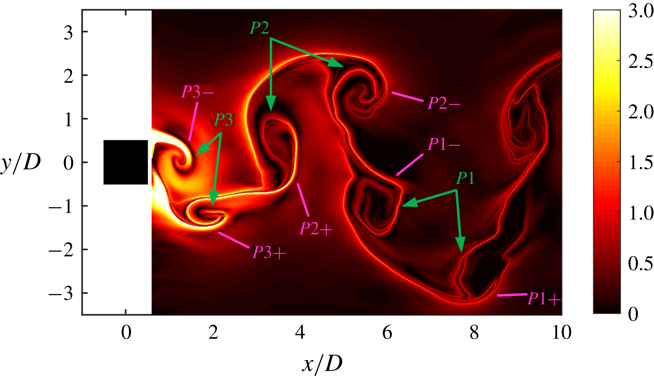
Figure 8 shows the FTLE field downstream of the square cylinder at an instant for $f_{e}/f_{0}=2.0$ . The boundaries of the wake vortices are clearly identified, elucidating the process of vortex evolution and pairing. Three wake vortex pairs, marked as $P1$ , $P2$ and $P3$ , can be observed within the current field of view. Each vortex pair consists of two counter-rotating vortices that are from the upper and lower shear layers, respectively. For example, the first vortex $P1+$ of the pair $P1$ is shed from the lower shear layer, the second vortex $P1-$ comes from the upper shear layer, and $P2-$ and $P2+$ are detached from the upper and lower shear layers, respectively. In other words, the two vortices shed from the same-side shear layer within half of the wake vortex-shedding cycle in figure 7 move apart and separately become a part of two different wake vortex pairs, denoting a 2P vortex-shedding mode. The similar flow pattern of a 2P mode was also observed in the wake of an oscillating airfoil (Koochesfahani Reference Koochesfahani1989; Schnipper, Andersen & Bohr Reference Schnipper, Andersen and Bohr2009) and the wake of an oscillating cylinder (Williamson & Roshko Reference Williamson and Roshko1988; Brika & Laneville Reference Brika and Laneville1993; Zdero, Turan & Havard Reference Zdero, Turan and Havard1995; Williamson & Govardhan Reference Williamson and Govardhan2008), in which the models are all movable. However, the square cylinder is fixed in our study, the 2P mode is induced by the upstream disturbances from the synthetic jet.

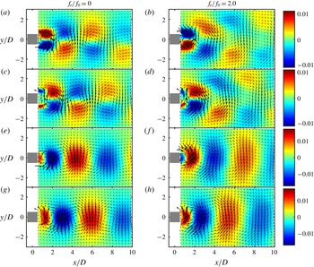
The first and second POD modes for the natural case and the case of $f_{e}/f_{0}=2.0$ are compared in figure 9 to reveal the variation in the wake vortex shedding. For the natural case, the first two POD modes contain 60 % of the total energy, with the first and second modes accounting for 31 % and 29 %, respectively. The first two POD modes for $f_{e}/f_{0}=2.0$ have comparable energy proportions to those for the natural case, with the first and second modes representing 32 % and 30 % of the total energy, respectively. It follows that the first pair of POD modes plays a dominant role in the wake for both of the cases. With regard to the spatial distribution of POD modes in these two cases, the modes of the streamwise velocity and the vertical velocity are antisymmetric and symmetric about the $y$ -axis, respectively, and the signs are distributed alternately along the streamwise direction, indicating the antisymmetric wake vortex-shedding mode. For the first two POD modes of streamwise velocity, the patterns exhibit a parallel distribution in the regions of $y>0$ and $y<0$ for the natural case, while their vertical spacing becomes larger as $x$ increases for $f_{e}/f_{0}=2.0$ . For the first two POD modes of vertical velocity, the patterns for $f_{e}/f_{0}=2.0$ cover a wider range in the $y$ direction than those for the natural case. The differences can be ascribed to the fact that the counter-rotating vortex pairs generated for $f_{e}/f_{0}=2.0$ gradually move away from the wake centre line as they convect downstream, which was once reported in the work of Williamson & Roshko (Reference Williamson and Roshko1988) and Brika & Laneville (Reference Brika and Laneville1993).

Figure 8.

Finite-time Lyapunov exponent field based on the POD reconstructed velocity field at an instant for $f_{e}/f_{0}=2.0$ .

Figure 9.

The first two POD modes for the natural case (a,c,e,g) and for the case of $f_{e}/f_{0}=2.0$  (b,d,f,h). (a,b) The first POD mode of streamwise velocity, (c,d) the second POD mode of streamwise velocity, (e,f) the first POD mode of vertical velocity, (g,h) the second POD mode of vertical velocity.

When the excitation frequency is increased to $f_{e}/f_{0}=3.4$ , the blowing velocity at the slot exit is relatively high. There are still two vorticity concentration areas near the synthetic jet exit after the blowing cycle starts, although their shapes are not as regular as those in the former control cases, as shown at the instant $t_{0}$ in figure 10(a). The vorticity grows and extends $(t_{0}+0.28T)$ and later breaks into pieces, and the flow becomes turbulent, as shown at $t_{0}+0.73T$ . Because the excitation frequency in this case is relatively high, the vortices $S1$ and $S2$ are surrounded with the scattered vorticity from the last excitation cycle (see $t_{0}$ and $t_{0}+0.28T$ ), which has not dissipated completely or convected downstream of the square cylinder when the new excitation cycle starts. The synthetic jet was found to deflect toward only one side during the entire excitation process. The deflecting direction can be either the $+y$ or the $-y$ side. In order to get more information on the flow field, the phase averaging is conducted using the same method as in the case of $f_{e}/f_{0}=2.0$ . Figure 11 shows the phase-averaged streamlines superimposed on the phase-averaged spanwise vorticity $\unicode[STIX]{x1D714}_{z}D/U_{\infty }$ around the front and side surfaces of the square cylinder, where the synthetic jet deflects upward. With the higher excitation frequency, both the size and the strength of the synthetic jet vortex pair increase obviously. Note that the upper vortex with negative vorticity tends to move upward and round the upper front corner of the square cylinder, with an evident vertical displacement. However, the lower synthetic jet vortex shows little position change in the $y$ direction. The synthetic jet vortex pair later loses its coherence and breaks down due to the high momentum. Driven by the free stream, discrete negative vorticity convects downstream in the vicinity of the top surface of square cylinder, while positive vorticity drifts to the region near the slot exit. As presented by the streamlines, the behaviour of the synthetic jet vortices in this case has a positive effect on suppressing the flow separation. When the synthetic jet vortices have fully developed ( $\unicode[STIX]{x1D6F7}=140^{\circ }$ and $\unicode[STIX]{x1D6F7}=230^{\circ }$ ), induced by the downwash motion of the upper vortex, the streamlines become attached on the forepart of the top surface. Not like that for the natural case, the separation point (only the upper one can be observed in figure 11) is not fixed at the front corner of the square cylinder, but moves downstream with the development of the synthetic jet vortex. The separation region near the side surface disappears when the synthetic jet vortices are really weak $(\unicode[STIX]{x1D6F7}=50^{\circ })$ and after the synthetic jet vortices lose coherence $(\unicode[STIX]{x1D6F7}=320^{\circ })$ .

Figure 10.

Evolution of the instantaneous flow structures around the front surface of the square cylinder for $f_{e}/f_{0}=3.4$ . The initial time $t_{0}$ is arbitrary. Here $T$ is one excitation period of the synthetic jet. (a) The instantaneous spanwise vorticity $\unicode[STIX]{x1D714}_{z}D/U_{\infty }$ obtained by PIV, (b) streamwise velocity history (in black) and the fitting sine function (in red) at $(x/D,y/D)=(-0.55,0)$ measured by PIV, with points $\unicode[STIX]{x2460}$ to $\unicode[STIX]{x2462}$ corresponding to the three instants in (a).

To further confirm the above variation in the flow separation, the phase-averaged streamwise velocity $\hat{U} /U_{\infty }$ located in $-0.5\leqslant x/D\leqslant 0.5$ and $y/D=0.625$ is extracted for the natural case and the case of $f_{e}/f_{0}=3.4$ , as displayed in figure 12. The black dashed line shows the positions where $\hat{U} /U_{\infty }$ is equal to zero. The phases in figures 12(a) and 12(b) are in accordance with those in figures 2 and 11, respectively. For the natural case in figure 12(a), the length of $\hat{U} /U_{\infty }<0$ undergoes a first increasing and then decreasing process with phase during one wake vortex-shedding cycle. This is because the separated shear layers oscillate periodically under the influence of the alternate wake vortex shedding (Huang, Hsu & Chen Reference Huang, Hsu and Chen2017). For $f_{e}/f_{0}=3.4$ in figure 12(b), the area of $\hat{U} /U_{\infty }<0$ is greatly reduced and its central position (presented by the dashed line in magenta) appears farther downstream with phase, consistent with the downstream movement of separation region in figure 11. No periodic wake vortex shedding is observed for the current case of $f_{e}/f_{0}=3.4$ . With the control of the upstream synthetic jet, the flow in the wake loses its coherence and the vorticity distributes discretely. A similar mode was observed in the range $4.3<R<8.3$ in the flow control using a continuous jet by Huang et al. (Reference Huang, Hsu and Chiu2014) where the continuous jet deflected to either side and broke up after a short distance from the slot; the flow in the wake also lost the periodicity.

Figure 11.

Phase-averaged streamlines overlaid on the phase-averaged spanwise vorticity $\unicode[STIX]{x1D714}_{z}D/U_{\infty }$ upstream of the rear surface of the square cylinder within one excitation cycle for $f_{e}/f_{0}=3.4$ .

Figure 12.

Variation of phase-averaged streamwise velocity $\hat{U} /U_{\infty }$ extracted from the position of $-0.5\leqslant x/D\leqslant 0.5$ and $y/D=0.625$ with phase. (a) One wake vortex-shedding cycle for $f_{e}/f_{0}=0$ , (b) one excitation cycle for $f_{e}/f_{0}=3.4$ .

As a comparison between our results and those in Huang et al. (Reference Huang, Hsu and Chiu2014), both the synthetic jet and the continuous jet present a swinging motion attached to the front surface of the square cylinder when the exit velocity is low, and they deflect toward either side as the exit velocity becomes larger. The continuous jet remains near the central axis for most of the time at a high injection ratio $(R>8.3)$ , while the exit velocity of the synthetic jet does not reach such a high value in our present study. Both of the injections are effective in suppressing the wake vortex shedding. If we define the ratio of the time-averaged blowing velocity over an excitation cycle $\overline{U_{0}}$ to the free-stream velocity $U_{\infty }$ as the injection ratio of the synthetic jet, then the wake vortices lose periodicity at $R=1\;(f_{e}/f_{0}=3.4)$ . For the continuous jet, however, the periodic wake vortex shedding disappears at $R>4.3$ . In addition, Huang et al. (Reference Huang, Hsu and Chiu2014) found that the free-stream Reynolds number tested in their study $(Re~1628{-}13\,000)$ had little effect on the values of the injection ratio between characteristic flow regimes. It can thus be inferred that the synthetic jet is more efficient in suppressing the wake vortex shedding of the square cylinder than the continuous jet when placed at the front surface.

3.2 Power spectrum analysis based on Fourier mode decomposition

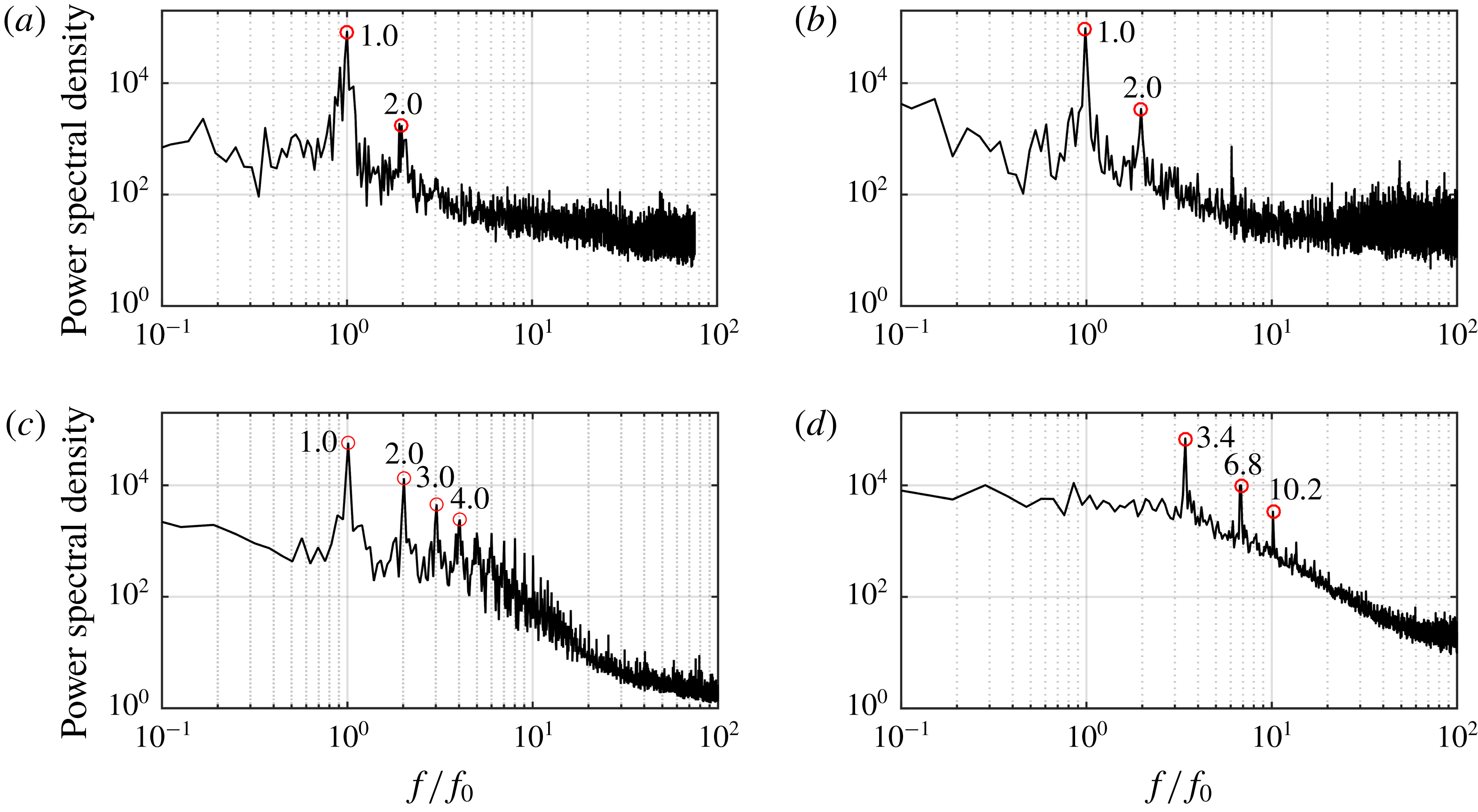
Fourier mode decomposition (FMD), proposed by Ma et al. (Reference Ma, Feng, Pan, Gao and Wang2015), is an effective method in detecting the characteristic frequencies of the global flow based on the global power spectrum. To implement this method, firstly the discrete Fourier transformation (DFT) is applied to the signal at each sampling point to get a matrix sequence with global spectral information. Then the global power spectrum is obtained by calculating the statistic of this matrix sequence. For more concrete calculation information, one can refer to the work of Ma et al. (Reference Ma, Feng, Pan, Gao and Wang2015) and Wang et al. (Reference Wang, Feng, Wang and Li2018). In the current study, the FMD algorithm is used to get the characteristic frequencies for the upstream flow field and the wake flow field, respectively, revealing the comparative relation between the inherent flow instability and the instability introduced by the synthetic jet. The FMD spectra of the streamwise velocity for different cases are shown in figures 13 and 14, with the computational domain of $-2.5\leqslant x/D\leqslant 0.5$ , $-2.5\leqslant y/D\leqslant 2.5$ and $0.5\leqslant x/D\leqslant 8$ , $-3.5\leqslant y/D\leqslant 3.5$ , respectively. According to the algorithm, the frequency resolution of FMD is the same as that of DFT. With a continuous sampling of 5457 frames and a sampling rate of 50, 60, 100 and 150 Hz for $f_{e}/f_{0}=0$ , 1.0, 2.0, 3.4, respectively, the corresponding frequency resolutions of FMD to the above cases are 0.009, 0.011, 0.018 and 0.027 Hz, and 0.03, 0.04, 0.06 and 0.09, respectively, if normalized by $f_{0}$ .

For the natural case, the wake instability is contributed by the von Kármán vortex shedding, thus a dominant frequency of $f_{0}$ is shown on the FMD spectrum in figure 14(a). The upstream flow field is under the influence of the upstream propagating signal from the wake (Huang et al. Reference Huang, Hsu and Chiu2014), thus a peak frequency identical to $f_{0}$ and a harmonic of $2f_{0}$ appear on the spectrum in figure 13(a).

Although with the synthetic jet excitation, the spectra for $f_{e}/f_{0}=1.0$ are very similar to those for the natural case. The downstream flow field still shows a peak value at $f_{0}$ (figure 14 b), because the synthetic jet is too weak to control the wake in this case, as described in figure 5. Deduced from the dominant frequency of $f_{0}$ on the spectrum in figure 13(b), the flow in the upstream is still governed by the feedback signal of wake vortices.

For $f_{e}/f_{0}=2.0$ , the dominant frequency of the upstream flow field remains at $f_{0}$ , and its high-order harmonics, even up to the value of $10f_{0}$ , can be clearly identified from the spectrum (figure 13 c), which is really different from the spectra for $f_{e}/f_{0}=0$ (figure 13 a) and $f_{e}/f_{0}=1.0$ (figure 13 b). A prominent peak of $f_{0}$ and sub-peaks of $2f_{0}$ and $3f_{0}$ are resolved on the FMD spectrum of the wake, as shown in figure 14(c). These results can be linked with the flow behaviour: the momentum of the synthetic jet becomes larger in this case, the influence of the synthetic jet on the flow field increases accordingly. However, it is not strong enough to take over the dominant position of the inherent flow instability. As described in figures 7 and 8, the wake vortex pairs generate and convect downstream alternately with a frequency of $f_{0}$ , resulting in the main peak of $f_{0}$ in figure 14(c). In the upstream, the synthetic jet deflects to the top and bottom side of the square cylinder alternately, and it takes the synthetic jet vortices two excitation periods to complete an entire developing cycle. Thus, the upstream flow field presents a dominant frequency at half of the excitation frequency, which is also equal to the natural vortex-shedding frequency.

Figure 13.

Fourier mode decomposition spectra of streamwise velocity in the upstream flow field at different excitation frequencies: (a)  $f_{e}/f_{0}=0$ , (b)  $f_{e}/f_{0}=1.0$ , (c)  $f_{e}/f_{0}=2.0$ , (d)  $f_{e}/f_{0}=3.4$ .

Figure 14.

Fourier mode decomposition spectra of streamwise velocity in the wake at different excitation frequencies: (a)  $f_{e}/f_{0}=0$ , (b)  $f_{e}/f_{0}=1.0$ , (c)  $f_{e}/f_{0}=2.0$ , (d)  $f_{e}/f_{0}=3.4$ .

As shown in figure 13(d), the dominant frequency of the upstream flow field for $f_{e}/f_{0}=3.4$ is identical to the excitation frequency $f_{e}\;(3.4f_{0})$ . Obvious peaks also appear at the multiples of the excitation frequency, $2f_{e}\;(6.8f_{0})$ and $3f_{e}\;(10.2f_{0})$ , and no indication of the characteristic frequency around $f_{0}$ can be found. As a result of the periodic flow behaviour in figure 11, the disturbances induced by synthetic jet govern the upstream flow field, and the wake vortex shedding is suppressed effectively. The peak near the natural vortex-shedding frequency disappears on the spectrum of the wake, as displayed in figure 14(d). There is a local peak at the location of the excitation frequency $(3.4f_{0})$ , indicating that the influence of the synthetic jet extends to the region downstream.

In the experiment by Huang et al. (Reference Huang, Hsu and Chiu2014), the characteristic frequencies at single points in the upstream and the wake were detected simultaneously. For both of the injections, the flow fields are governed by the periodic wake vortex shedding when the injection momentum is small. As the injection momentum increases, the wake finally loses the periodicity in the range $R>4.3$ for the continuous jet and at $f_{e}/f_{0}=3.4$ for the synthetic jet. Due to the features of the synthetic jet being a time-periodic actuation but the continuous jet a steady excitation, the upstream flow field is finally locked on the excitation frequency when controlled with the synthetic jet, but has no periodic oscillation when controlled with the continuous jet (Huang et al. Reference Huang, Hsu and Chiu2014).

3.3 Statistical characteristics of flow field

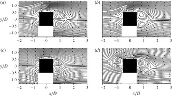
Figure 15 demonstrates the time-averaged streamlines around the square cylinder at different excitation frequencies. Without control, the flow splits into two streams and heads towards the two front corners, respectively, after contacting with the front surface of the square cylinder (figure 15 a). Then the flow separates at the front corners, forming separation bubbles beside the side surfaces and a large recirculation region in the wake. The recirculation region is symmetric about the wake centre line. For the control cases of $f_{e}/f_{0}=1.0$ (figure 15 b) and $f_{e}/f_{0}=2.0$ (figure 15 c), the streamlines in the vicinity of the slot present a slight difference due to the motion of the synthetic jet. The time-averaged flow patterns after the separation do not change much compared with those for the natural case. The size of the recirculation region downstream of the square cylinder decreases with increasing excitation frequency, indicating a more and more effective control effect of the synthetic jet. A similar variation trend of time-averaged streamlines near the slot and in the wake with the excitation frequency was obtained for $f_{e}/f_{0}\leqslant 2.08$ in the flow control of a circular cylinder conducted by Feng & Wang (Reference Feng and Wang2014). At a higher excitation frequency of $f_{e}/f_{0}=3.4$ (figure 15 d), a large recirculation region with two counter-rotating vortices is induced in the upstream, pushing the mean front stagnation point more upstream. Corresponding to the deflection state of the synthetic jet in figure 11, the centre line of the recirculation region in the upstream is inclined to the $+y$ direction. The envelope is closed at the bottom and is open at the top. There is still an obvious recirculation region in the wake with the centre line inclined to the $-y$ direction. A similar symmetry-breaking bifurcation was reported in the numerical study of Kim et al. (Reference Kim, Yang and Eom2003), where a planar jet with $R=1.54$ was exerted on the front surface of a square cylinder. With the current spatial resolution, no apparent flow separation beside the top surface can be observed from the time-averaged streamlines for $f_{e}/f_{0}=3.4$ , which seems reasonable if the variation of the separation bubble with phase in figure 11 is considered.

Figure 15.

Time-averaged streamlines around the square cylinder at different excitation frequencies: (a)  $f_{e}/f_{0}=0$ , (b)  $f_{e}/f_{0}=1.0$ , (c)  $f_{e}/f_{0}=2.0$ , (d)  $f_{e}/f_{0}=3.4$ .

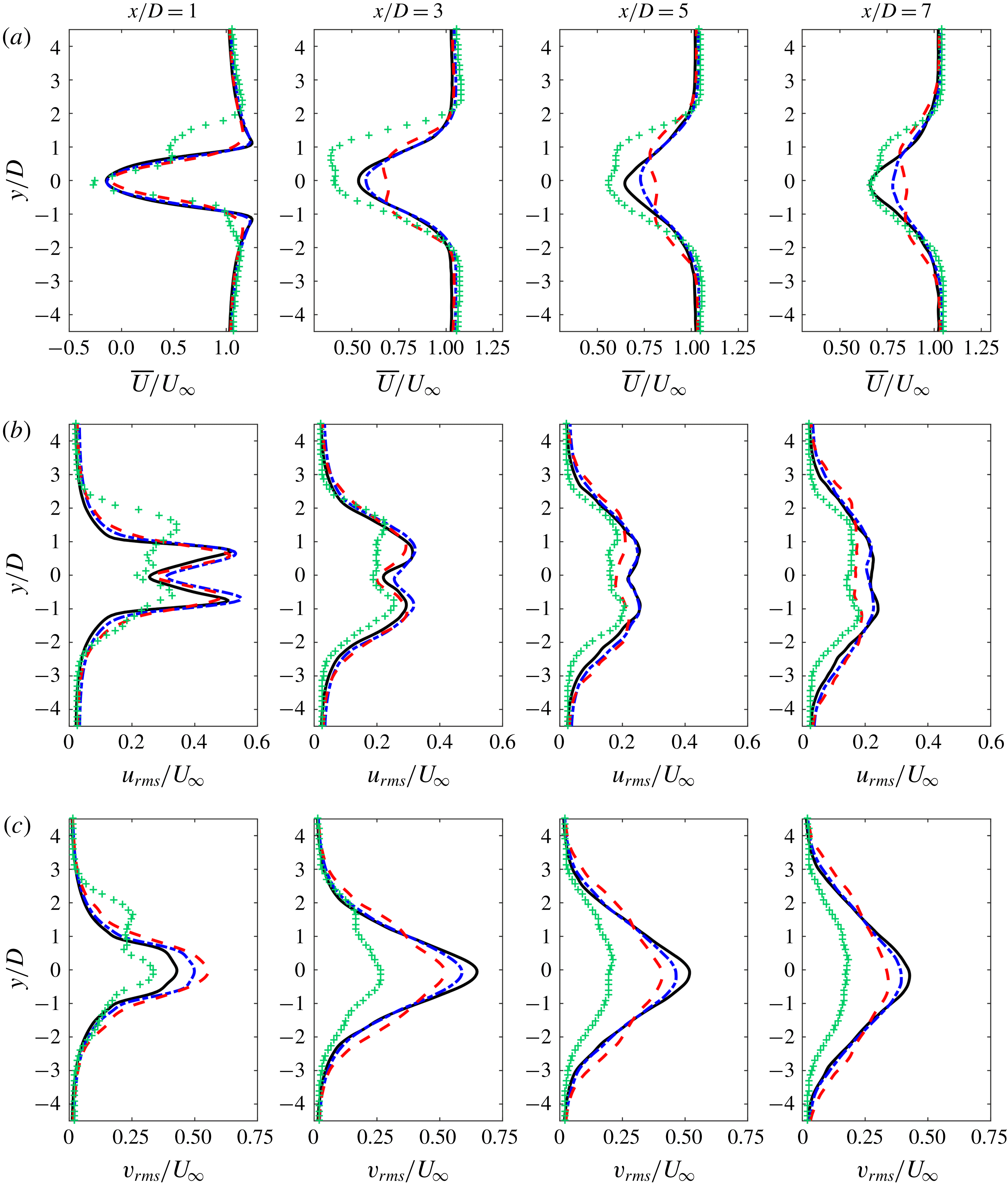
Figure 16(a) compares the distributions of the time-averaged streamwise velocity $\overline{U}/U_{\infty }$ at different streamwise locations for different cases. At $x/D=1$ , each of the profiles has the streamwise velocity deficit. Due to the backflow in the near wake, which has been demonstrated in figure 15, the minimum values of $\overline{U}/U_{\infty }$ are all less than zero, and the values of $\overline{U}/U_{\infty }$ for $f_{e}/f_{0}\leqslant 2.0$ are quite close. For $f_{e}/f_{0}=3.4$ , the maximum velocity deficit is a little larger than that of the other cases. Besides, another local minimum appears near the location of $y/D=1$ , affected by the downstream convection of the synthetic jet vortices. Further downstream, the streamwise velocity deficit in the wake recovers gradually, and the maximum velocity deficit for $f_{e}/f_{0}\leqslant 2.0$ decreases with increasing the excitation frequency. Note that two minima appear on the profiles downstream from $x/D=3$ for $f_{e}/f_{0}=2.0$ , which can be related to the change of the wake vortex-shedding mode. A similar profile of mean velocity was obtained in the wake of an oscillating airfoil when the wake vortex shedding also presented the 2P mode (Koochesfahani Reference Koochesfahani1989). Moreover, the expansion of the velocity deficit region in the $y$ direction for $f_{e}/f_{0}=2.0$ is wider than that of the natural case downstream from $x/D=3$ , consistent with the description in figure 9. Roughly speaking, the value of $\overline{U}/U_{\infty }$ in the wake for $f_{e}/f_{0}=3.4$ is smaller than that in the other cases.

As shown in figure 16(b), all the profiles of the streamwise velocity fluctuation $u_{rms}/U_{\infty }$ for the cases of $f_{e}/f_{0}\leqslant 2.0$ are double-peak distributions. The two peaks are related to the shear layers and the wake vortices (van Oudheusden et al. Reference van Oudheusden, Scarano, van Hinsberg and Watt2005; He et al. Reference He, Li and Wang2014). Differently, three peaks can be found on the profile for $f_{e}/f_{0}=3.4$ at $x/D=1$ . The upper one is associated with the convection of the discrete synthetic jet vortex, and the middle and the lower ones, which are relatively small, correspond to the shear layers around the rear corners of the square cylinder. The peak values reduce gradually with the streamwise location downstream for all the cases. The streamwise velocity fluctuations for $f_{e}/f_{0}=0$ and $f_{e}/f_{0}=1.0$ are nearly at the same level, in comparison, the $u_{rms}$ value for $f_{e}/f_{0}=2.0$ is slightly lower in the downstream. The case of $f_{e}/f_{0}=3.4$ always has the minimum streamwise velocity fluctuation.

Figure 16.

Distributions of velocity statistics at different streamwise locations for different cases. (a) Dimensionless time-averaged streamwise velocity $\overline{U}/U_{\infty }$ , (b) dimensionless root-mean-square of streamwise velocity fluctuation $u_{rms}/U_{\infty }$ , (c) dimensionless root-mean-square of vertical velocity fluctuation $v_{rms}/U_{\infty }$ . Solid line in black, $f_{e}/f_{0}=0$ ; dash-dotted line in blue, $f_{e}/f_{0}=1.0$ ; dashed line in red, $f_{e}/f_{0}=2.0$ ; plus symbol in green, $f_{e}/f_{0}=3.4$ .

Figure 16(c) displays the distributions of the vertical velocity fluctuation $v_{rms}/U_{\infty }$ . For $f_{e}/f_{0}\leqslant 2.0$ , peak values appear at $y=0$ , and the profiles are symmetric about the centre line. Affected by the behaviour of the synthetic jet, an additional peak appears on the profile for $f_{e}/f_{0}=3.4$ in the near wake. Further, the maximum of $v_{rms}/U_{\infty }$ at each streamwise location is extracted and its variation along the streamwise direction is presented in figure 17. It can be seen that $v_{rms\cdot max}/U_{\infty }$ firstly increases and then decreases with the location downstream. For $f_{e}/f_{0}\leqslant 2.0$ , as the excitation frequency increases, the peak value of $v_{rms\cdot max}/U_{\infty }$ appears closer to the square cylinder, indicating a reduction of the vortex formation length. Besides, the $v_{rms\cdot max}/U_{\infty }$ level increases with the excitation frequency in the near wake for $f_{e}/f_{0}\leqslant 2.0$ , while the trend is opposite in the downstream. The synthetic jet shows the best control effect on reducing the vertical velocity fluctuation at the excitation frequency of $f_{e}/f_{0}=3.4$ , as the $v_{rms}$ level in figure 16 and $v_{rms\cdot max}$ level in figure 17 are much lower than those for the other cases. The variations in $v_{rms\cdot max}/U_{\infty }$ can also be reflected in the profiles of $v_{rms}/U_{\infty }$ at the given streamwise locations in figure 16(c).

Figure 17.

Streamwise variation of maximum vertical velocity fluctuation $v_{rms\cdot max}/U_{\infty }$ at different excitation frequencies.