1 Introduction
Non-invasive estimation or reconstruction of instantaneous flows is a generic problem in fluid dynamics. In particular, estimation or reconstruction of fully developed turbulence using the information only on the boundaries is a challenging problem relevant to various applications (see Bewley Reference Bewley2001; Brunton & Noack Reference Brunton and Noack2015, for example). Wide spectra of the length and time scales generate many degrees of freedom (i.e. mutually less correlated motions), and poor correlation between the motion near the wall and that outside the boundary layer prevents accessibility to large-scale structures based on the information on the wall. In other words, motions in the vicinity of the wall dominate fluctuating components measured on the wall.
Because of such difficulties in turbulence estimation and the limitation of even the state-of-the-art measurement capability (especially in terms of accuracy and spatial resolution), the main frame of current research is computational fluid dynamics (CFD). We find, for example, various types of flows in recent estimation studies (Chevalier, Hœpffner & Henningson Reference Chevalier, Hœpffner and Henningson2007; Jones et al. Reference Jones, Kerrigan, Morrison and Zaki2011; Lasagna & Tutty Reference Lasagna and Tutty2015) as well as past studies in a review article (Kim & Bewley Reference Kim and Bewley2007). Considering the current status and the ultimate application in experiments, the underlying assumptions would be that (i) the unsteady flow to be estimated during a certain period, called the ‘true solution’, is an exact solution to the governing equations solved by the CFD with a given geometry, (ii) we can take any statistics necessary for the estimation regarding the flow and the wall measurement equivalent to the true solution from the CFD (namely, we should not sample the flow field during the true solution but its statistics are available, for example from different ensembles), yet (iii) the measurement during the true solution is available only on the wall, potentially with the full resolution (although it can be noisy) and (iv) the initial condition is totally unknown. Some of the assumptions were unclear in several past studies, and they may have misled conclusions, as discussed later in §§ 2.1 and 3.2 and appendices A and D. In spite of these ideal assumptions, it is evident that the problem remains challenging.
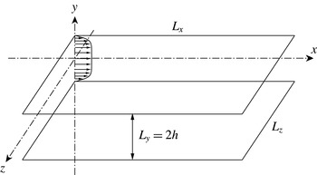
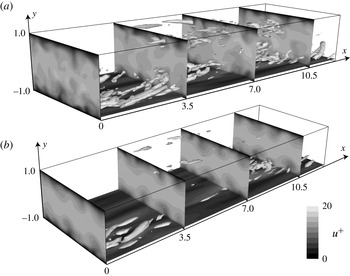
Flow geometry to be solved and the coordinate system.

Bewley and his colleagues (Bewley, Moin & Temam Reference Bewley, Moin and Temam2001; Högberg, Bewley & Henningson Reference Högberg, Bewley and Henningson2003; Bewley & Protas Reference Bewley and Protas2004; Chevalier et al.
Reference Chevalier, Hœpffner, Bewley and Henningson2006; Colburn, Cessna & Bewley Reference Colburn, Cessna and Bewley2011) have studied such flow estimation problems by solving turbulent channel flows with periodic boundary conditions using direct numerical simulation (DNS) primarily at the friction Reynolds number of
 $Re_{\unicode[STIX]{x1D70F}}=100$
: they estimated unsteady flows based on noisy wall measurement, equivalent to the wall shear stresses in the streamwise and spanwise directions as well as the wall pressure over the entire wavenumber space. Figure 1 illustrates the flow geometry and the coordinate system. Such a configuration is simple and generic but possesses essential features for non-invasive estimation of fully developed turbulence; namely, we observe a cascade of eddies in a wall-bounded space only through measurable quantities on the wall. They have applied several data assimilation methods including an adjoint-based variational technique (Bewley et al.
Reference Bewley, Moin and Temam2001; Bewley & Protas Reference Bewley and Protas2004) and sequential techniques (Chevalier et al.
Reference Chevalier, Hœpffner, Bewley and Henningson2006; Colburn et al.
Reference Colburn, Cessna and Bewley2011). In particular, the latter, namely the Kalman filter (Kalman Reference Kalman1960) in their study, consists of a prediction step involving a dynamical system and an update step governed by the instantaneous wall measurement. In contrast to the DNS, which nonlinearly solves a state vector yet only with dimensions of
 $3N_{grid}$
, with
 $N_{grid}$
being the grid counts in the physical or Fourier space, the Kalman filter must additionally advance a covariance matrix with a dimension of
 $3N_{grid}\times 3N_{grid}$
in time and approximately invert a matrix of this size even for a linear time-invariant system in principle (there are ways to avid direct inversion of the matrix, such as a sequential processing (Bucy & Joseph Reference Bucy and Joseph1968)). In addition to such high computational cost, correlations across the entire input/forcing points (or the corresponding wavenumbers) are necessary for all quantities, spanning huge dimensions and requiring extensive sampling time. The ensemble Kalman filter (Evensen Reference Evensen1994) can also circumvent such large matrix calculation, but instead needs simultaneous simulations of ensemble members, typically more than
 $50$
.
These reconstruction studies may give us an impression that such sequential data assimilation techniques owe their success (in particular, Colburn et al. (Reference Colburn, Cessna and Bewley2011) reported exceptional success in turbulence estimation using the ensemble Kalman filter) primarily to the prediction step solving the governing equations for the state vector and its covariance matrix, rather than the update step given by the instantaneous measurement. However, these studies have not evaluated the contribution of each step; namely, it is unclear if the instantaneous estimation (i.e. the update step) is sufficient or the sequential prediction is crucial. In addition, filtering of the measurement noise relies on the assumption of ‘known’ statistics (for the noise not for the true solution), leaving a question of practicality. Moreover, large dimensions in the spatial correlation matrix comprise many degrees of freedom, and the number of sampled snapshots must far exceed the dimensions of the correlation matrix; otherwise, the correlation matrix merely ‘memorizes’ the flow patterns during the sampling duration. Such reconstruction works only for flows composed of motions similar to those occurred during the sampling time but would fail to estimate different phases of flows even under the same condition.
Our goal is to clarify the contributions from the two essential steps in sequential turbulent flow estimation using simpler approaches: this study re-tackles the same benchmark flow estimation problem of a turbulent channel flow at
 $Re_{\unicode[STIX]{x1D70F}}=100$
with periodic boundary conditions by Chevalier et al. (Reference Chevalier, Hœpffner, Bewley and Henningson2006). For the update step, we apply linear stochastic estimation (Adrian & Moin Reference Adrian and Moin1988) to the wall measurement over the entire wavenumber space. This technique provides the best estimate of instantaneous velocity components at any points in space in a least-squares sense. We then proportionally feed these velocity fields via the body-force term and solve the full incompressible Navier–Stokes equations using DNS for the prediction step. These two steps constitute a simple state observer. By evaluating the degree of agreement with the true solution at each step, we can separate the effect of instantaneous estimation from the prediction step in a sequential-type data assimilation approach.
The results uncover important implications which were not transparent in the previous studies: we show poor correlations between the measured quantities on the wall and the velocity components in the flow as well as limited improvement by inclusion of time derivatives of the measured quantities, justifying our linear stochastic estimation approach. The analysis of the measurement noise demonstrates that even a simple sequential technique can effectively suppress uncorrelated noise, by merely increasing the frequency of the feedback. Accordingly, the instantaneous estimation by the linear stochastic estimation is sufficient to reconstruct the velocity field near the wall (within the wall units of
 $y^{+}\lesssim 20$
) in the degree reported by Chevalier et al. (Reference Chevalier, Hœpffner, Bewley and Henningson2006) using the extended Kalman filter; furthermore, not only the simple observer solving the nonlinear dynamical system but also the ensemble Kalman filter performed in this study provide limited improvement in the log layer. These results affirm the inherent difficulty of turbulent flow estimation due to weak coherence between fluctuations in the viscous sublayer and strong motions in the buffer layer. From the series of the analyses, we can also deduce potential hurdles that have not been quite resolved by the sequential data assimilation approaches in the past studies.
The rest of the paper is organized as follows. After the introduction, the governing equations and the wall measurements are formulated, followed by the descriptions of linear stochastic estimation and the body-force term. The computational methods, i.e. DNS, are then briefly summarized, and the procedure of the sampling is carefully stated. In the results and discussions, fundamental flow features are first observed, the instantaneous estimation using the linear stochastic estimation is then analysed and the effects of the body-force feedback in the observer to the estimation are eventually discussed. Finally, the conclusions and implications are addressed referring to the past studies. Independent analyses of the noise filtering effect, linear stochastic estimation including time derivatives of the wall measurement, and the ensemble Kalman filter are performed in the appendices. In addition, the no-slip wall treatment for a spectral method with a collocation technique is explained in an appendix.
2 Formulation
2.1 The governing equations and the wall measurement
This study solves the incompressible Navier–Stokes equations to compute the true solution, to take its statistics (e.g. time averages and correlations for linear stochastic estimation as well as evaluation of the agreement) and to advance prediction steps in the observer. We non-dimensionalize the system of the equations by the channel half-height,
 $h$
, the constant density,
 $\unicode[STIX]{x1D70C}$
, and the friction velocity,
 $u_{\unicode[STIX]{x1D70F}}\equiv \sqrt{\bar{\unicode[STIX]{x1D70F}}_{w}/\unicode[STIX]{x1D70C}}$
(
 $\bar{\unicode[STIX]{x1D70F}}_{w}$
being the mean wall shear stress), and express it in three dimensions as:
 $$\begin{eqnarray}\displaystyle \frac{\unicode[STIX]{x2202}u}{\unicode[STIX]{x2202}t}+u\frac{\unicode[STIX]{x2202}u}{\unicode[STIX]{x2202}x}+v\frac{\unicode[STIX]{x2202}u}{\unicode[STIX]{x2202}y}+w\frac{\unicode[STIX]{x2202}u}{\unicode[STIX]{x2202}z}+\frac{\unicode[STIX]{x2202}p}{\unicode[STIX]{x2202}x}-\frac{1}{Re_{\unicode[STIX]{x1D70F}}}\unicode[STIX]{x1D6FB}^{2}u & = & \displaystyle 0,\end{eqnarray}$$
 $$\begin{eqnarray}\displaystyle \frac{\unicode[STIX]{x2202}v}{\unicode[STIX]{x2202}t}+u\frac{\unicode[STIX]{x2202}v}{\unicode[STIX]{x2202}x}+v\frac{\unicode[STIX]{x2202}v}{\unicode[STIX]{x2202}y}+w\frac{\unicode[STIX]{x2202}v}{\unicode[STIX]{x2202}z}+\frac{\unicode[STIX]{x2202}p}{\unicode[STIX]{x2202}y}-\frac{1}{Re_{\unicode[STIX]{x1D70F}}}\unicode[STIX]{x1D6FB}^{2}v & = & \displaystyle 0,\end{eqnarray}$$
 $$\begin{eqnarray}\displaystyle \frac{\unicode[STIX]{x2202}w}{\unicode[STIX]{x2202}t}+u\frac{\unicode[STIX]{x2202}w}{\unicode[STIX]{x2202}x}+v\frac{\unicode[STIX]{x2202}w}{\unicode[STIX]{x2202}y}+w\frac{\unicode[STIX]{x2202}w}{\unicode[STIX]{x2202}z}+\frac{\unicode[STIX]{x2202}p}{\unicode[STIX]{x2202}z}-\frac{1}{Re_{\unicode[STIX]{x1D70F}}}\unicode[STIX]{x1D6FB}^{2}w & = & \displaystyle 0,\end{eqnarray}$$
 $$\begin{eqnarray}\frac{\unicode[STIX]{x2202}u}{\unicode[STIX]{x2202}x}+\frac{\unicode[STIX]{x2202}v}{\unicode[STIX]{x2202}y}+\frac{\unicode[STIX]{x2202}w}{\unicode[STIX]{x2202}z}=0,\end{eqnarray}$$
where the friction Reynolds number is defined as
 $Re_{\unicode[STIX]{x1D70F}}\equiv u_{\unicode[STIX]{x1D70F}}h/\unicode[STIX]{x1D708}$
(
 $\unicode[STIX]{x1D708}$
being the kinematic viscosity). The full nonlinear Navier–Stokes equations are solved for all these processes although fluctuating quantities relative to the time-averaged mean flow are used for post-processing and analyses in this study.
As described later in § 3.1, all the computation and the post-processing are performed in the wavenumber space, in which the discrete Fourier transform is defined as
 $$\begin{eqnarray}\tilde{u} (t,k_{x},y,k_{z})\equiv \frac{1}{N_{x}N_{z}}\mathop{\sum }_{n_{x}=0}^{N_{x}-1}\mathop{\sum }_{n_{z}=0}^{N_{z}-1}u(t,x_{n_{x}},y,z_{n_{z}})\exp [-\text{i}(k_{x}x_{n_{x}}+k_{z}z_{n_{z}})].\end{eqnarray}$$
Here, the discrete points in space and the wavenumbers are given by
 $x_{n_{x}}\equiv n_{x}L_{x}/N_{x}$
and
 $z_{n_{z}}\equiv n_{z}L_{z}/N_{z}$
(
 $n_{x}\in [0,N_{x}-1]$
and
 $n_{z}\in [0,N_{z}-1]$
) as well as
 $k_{x}\equiv 2\unicode[STIX]{x03C0}m_{x}/L_{x}$
and
 $k_{z}\equiv 2\unicode[STIX]{x03C0}m_{z}/L_{z}$
(
 $m_{x}\in [-N_{x}/2,N_{x}/2-1]$
and
 $m_{z}\in [-N_{z}/2,N_{z}/2-1]$
), where
 $L_{x}$
and
 $L_{z}$
are the domain lengths (i.e. the spatial periodicity) in the streamwise and spanwise directions, respectively. It should be remarked that
 $\tilde{u} (-k_{x},-k_{z})=\tilde{u} ^{\ast }(k_{x},k_{z})$
, where
 $\ast$
denotes complex conjugate. The other velocity components are similarly Fourier transformed only in the two periodic directions.
On both sides of the wall (i.e.
 $y/h=\pm 1$
), shear stresses in the streamwise and spanwise directions as well as pressure are recorded over the entire wavenumbers in time:
 $$\begin{eqnarray}\left.\begin{array}{@{}l@{}}\displaystyle \tilde{\unicode[STIX]{x1D70F}}_{x}=\frac{1}{Re_{\unicode[STIX]{x1D70F}}}\frac{\unicode[STIX]{x2202}\tilde{u} }{\unicode[STIX]{x2202}y},\\ \displaystyle \tilde{\unicode[STIX]{x1D70F}}_{z}=\frac{1}{Re_{\unicode[STIX]{x1D70F}}}\frac{\unicode[STIX]{x2202}\tilde{w}}{\unicode[STIX]{x2202}y},\\ \displaystyle \tilde{p}.\end{array}\right\}\end{eqnarray}$$
Unlike the series of studies by the Bewley & Henningson group (Bewley et al. Reference Bewley, Moin and Temam2001; Högberg et al. Reference Högberg, Bewley and Henningson2003; Bewley & Protas Reference Bewley and Protas2004; Chevalier et al. Reference Chevalier, Hœpffner, Bewley and Henningson2006; Colburn et al. Reference Colburn, Cessna and Bewley2011), we measure these physical quantities instead of the transverse derivative of the wall-normal vorticity and the second transverse derivative of the vertical velocity (the wall pressure is the same). To compare the results with their studies, we perform necessary conversions.
One such example is the conversion for the random measurement noise. Chevalier et al. (Reference Chevalier, Hœpffner, Bewley and Henningson2006) imposed Gaussian white noise with zero mean on these three measured quantities across the entire wavenumber range. In appendix A, we attempt to examine equivalent measurement noise for evaluation of the filtering capability, but their normalizations associated with the measurement noise are unclear throughout the series of the papers (Hœpffner et al. Reference Hœpffner, Chevalier, Bewley and Henningson2005; Chevalier et al. Reference Chevalier, Hœpffner, Bewley and Henningson2006; Colburn et al. Reference Colburn, Cessna and Bewley2011). In reality, however, we can readily filter out uncorrelated noise by simply applying a sequential technique and separate core flow estimation problems from the measurement noise issue, as explained in appendix A. In the rest of the main part, we impose no measurement noise during sampling and also develop the estimation scheme without assuming measurement noise.
2.2 Linear stochastic estimation
We apply linear stochastic estimation (Adrian & Moin Reference Adrian and Moin1988) for the instantaneous estimation. As explained later, the correlation across different wavenumbers between the wall measurements and the velocity components in the flow is fairly small, while there is appreciable correlation across the opposite side of the wall measurements. Moreover, appendix B demonstrates that including time derivatives of the wall measurements improves the estimation only a little. Consequently, we express the estimated velocity (denoted by
 $\tilde{u} _{LSE}$
below) as linear summation of instantaneous measured quantities and minimize the least-squares error over time from the true solution (denoted by
 $\tilde{u} _{DNS}$
). The cost function for the streamwise velocity in the interior domain then defines
 $$\begin{eqnarray}\displaystyle J_{u} & \equiv & \displaystyle \mathop{\sum }_{n_{t}=1}^{N_{time}}\left|\left(a_{x}^{\ast }\tilde{\unicode[STIX]{x1D70F}}_{x}+a_{z}^{\ast }\tilde{\unicode[STIX]{x1D70F}}_{z}+a_{p}^{\ast }\tilde{p}\right)_{y=-h}+\left(a_{x}^{\ast }\tilde{\unicode[STIX]{x1D70F}}_{x}+a_{z}^{\ast }\tilde{\unicode[STIX]{x1D70F}}_{z}+a_{p}^{\ast }\tilde{p}\right)_{y=+h}-\tilde{u} _{DNS}\left(t_{n_{t}},k_{x},y,k_{z}\right)\right|^{2}\nonumber\\ \displaystyle & \equiv & \displaystyle \sum \left|\boldsymbol{a}^{\dagger }\cdot \tilde{\unicode[STIX]{x1D749}}\left(t_{n_{t}}\right)-\tilde{u} _{DNS}\left(t_{n_{t}}\right)\right|^{2}=\sum \left|\tilde{u} _{LSE}\left(t_{n_{t}}\right)-\tilde{u} _{DNS}\left(t_{n_{t}}\right)\right|^{2},\end{eqnarray}$$
where
 $\tilde{\unicode[STIX]{x1D749}}$
has six components including the streamwise and spanwise wall shear stresses as well as the wall pressure on both
 $y/h=\pm 1$
in the wavenumber space and
 $\boldsymbol{a}^{\dagger }$
consists of
 $a_{x}^{\ast }$
,
 $a_{z}^{\ast }$
and
 $a_{p}^{\ast }$
, which denote their coefficients (to be precise, their complex conjugate is taken for later convenience). We similarly define the cost functions for
 $v$
and
 $w$
, while we compute pressure via the observer. Although the acquired velocity field generally does not satisfy continuity, the Poisson equation in the observer rectifies it, as described later. Assuming the symmetry in the
 $y$
and
 $z$
directions as well as the homogeneity in the
 $x$
and
 $z$
directions for the turbulent statistics, we expect that the mean quantities vanish except for
 $u$
of
 $(k_{x},k_{z})=(0,0)$
, and (2.5) directly expresses the equation for the fluctuating components.
We determine the coefficients above by setting
 $\unicode[STIX]{x2202}J_{u}/a=0$
where
 $a$
is each of the six coefficients in
 $\boldsymbol{a}$
. Accordingly, the system of equations for each
 $(k_{x},y,k_{z})$
yields
 $$\begin{eqnarray}\boldsymbol{a}=\left(\overline{\tilde{\unicode[STIX]{x1D749}}\tilde{\unicode[STIX]{x1D749}}^{\dagger }}\right)_{6\times 6}^{-1}\overline{\tilde{\unicode[STIX]{x1D749}}\tilde{u} _{DNS}^{\ast }},\end{eqnarray}$$
where
 $\dagger$
expresses the complex conjugate transpose and the overbar the time average, and
 $$\begin{eqnarray}\left(\overline{\tilde{\unicode[STIX]{x1D749}}\tilde{\unicode[STIX]{x1D749}}^{\dagger }}\right)\equiv \left[\begin{array}{@{}cccccc@{}}\overline{\tilde{\unicode[STIX]{x1D70F}}_{x}|_{+h}\tilde{\unicode[STIX]{x1D70F}}_{x}^{\ast }|_{+h}} & \overline{\tilde{\unicode[STIX]{x1D70F}}_{x}|_{+h}\tilde{\unicode[STIX]{x1D70F}}_{z}^{\ast }|_{+h}} & \overline{\tilde{\unicode[STIX]{x1D70F}}_{x}|_{+h}\tilde{p}^{\ast }|_{+h}} & \overline{\tilde{\unicode[STIX]{x1D70F}}_{x}|_{+h}\tilde{\unicode[STIX]{x1D70F}}_{x}^{\ast }|_{-h}} & \overline{\tilde{\unicode[STIX]{x1D70F}}_{x}|_{+h}\tilde{\unicode[STIX]{x1D70F}}_{z}^{\ast }|_{-h}} & \overline{\tilde{\unicode[STIX]{x1D70F}}_{x}|_{+h}\tilde{p}^{\ast }|_{-h}}\\ \overline{\tilde{\unicode[STIX]{x1D70F}}_{z}|_{+h}\tilde{\unicode[STIX]{x1D70F}}_{x}^{\ast }|_{+h}} & \overline{\tilde{\unicode[STIX]{x1D70F}}_{z}|_{+h}\tilde{\unicode[STIX]{x1D70F}}_{z}^{\ast }|_{+h}} & \overline{\tilde{\unicode[STIX]{x1D70F}}_{z}|_{+h}\tilde{p}^{\ast }|_{+h}} & \overline{\tilde{\unicode[STIX]{x1D70F}}_{z}|_{+h}\tilde{\unicode[STIX]{x1D70F}}_{x}^{\ast }|_{-h}} & \overline{\tilde{\unicode[STIX]{x1D70F}}_{z}|_{+h}\tilde{\unicode[STIX]{x1D70F}}_{z}^{\ast }|_{-h}} & \overline{\tilde{\unicode[STIX]{x1D70F}}_{z}|_{+h}\tilde{p}^{\ast }|_{-h}}\\ \overline{\tilde{p}|_{+h}\tilde{\unicode[STIX]{x1D70F}}_{x}^{\ast }|_{+h}} & \overline{\tilde{p}|_{+h}\tilde{\unicode[STIX]{x1D70F}}_{z}^{\ast }|_{+h}} & \overline{\tilde{p}|_{+h}\tilde{p}^{\ast }|_{+h}} & \overline{\tilde{p}|_{+h}\tilde{\unicode[STIX]{x1D70F}}_{x}^{\ast }|_{-h}} & \overline{\tilde{p}|_{+h}\tilde{\unicode[STIX]{x1D70F}}_{z}^{\ast }|_{-h}} & \overline{\tilde{p}|_{+h}\tilde{p}^{\ast }|_{-h}}\\ \overline{\tilde{\unicode[STIX]{x1D70F}}_{x}|_{-h}\tilde{\unicode[STIX]{x1D70F}}_{x}^{\ast }|_{+h}} & \overline{\tilde{\unicode[STIX]{x1D70F}}_{x}|_{-h}\tilde{\unicode[STIX]{x1D70F}}_{z}^{\ast }|_{+h}} & \overline{\tilde{\unicode[STIX]{x1D70F}}_{x}|_{-h}\tilde{p}^{\ast }|_{+h}} & \overline{\tilde{\unicode[STIX]{x1D70F}}_{x}|_{-h}\tilde{\unicode[STIX]{x1D70F}}_{x}^{\ast }|_{-h}} & \overline{\tilde{\unicode[STIX]{x1D70F}}_{x}|_{-h}\tilde{\unicode[STIX]{x1D70F}}_{z}^{\ast }|_{-h}} & \overline{\tilde{\unicode[STIX]{x1D70F}}_{x}|_{-h}\tilde{p}^{\ast }|_{-h}}\\ \overline{\tilde{\unicode[STIX]{x1D70F}}_{z}|_{-h}\tilde{\unicode[STIX]{x1D70F}}_{x}^{\ast }|_{+h}} & \overline{\tilde{\unicode[STIX]{x1D70F}}_{z}|_{-h}\tilde{\unicode[STIX]{x1D70F}}_{z}^{\ast }|_{+h}} & \overline{\tilde{\unicode[STIX]{x1D70F}}_{z}|_{-h}\tilde{p}^{\ast }|_{+h}} & \overline{\tilde{\unicode[STIX]{x1D70F}}_{z}|_{-h}\tilde{\unicode[STIX]{x1D70F}}_{x}^{\ast }|_{-h}} & \overline{\tilde{\unicode[STIX]{x1D70F}}_{z}|_{-h}\tilde{\unicode[STIX]{x1D70F}}_{z}^{\ast }|_{-h}} & \overline{\tilde{\unicode[STIX]{x1D70F}}_{z}|_{-h}\tilde{p}^{\ast }|_{-h}}\\ \overline{\tilde{p}|_{-h}\tilde{\unicode[STIX]{x1D70F}}_{x}^{\ast }|_{+h}} & \overline{\tilde{p}|_{-h}\tilde{\unicode[STIX]{x1D70F}}_{z}^{\ast }|_{+h}} & \overline{\tilde{p}|_{-h}\tilde{p}^{\ast }|_{+h}} & \overline{\tilde{p}|_{-h}\tilde{\unicode[STIX]{x1D70F}}_{x}^{\ast }|_{-h}} & \overline{\tilde{p}|_{-h}\tilde{\unicode[STIX]{x1D70F}}_{z}^{\ast }|_{-h}} & \overline{\tilde{p}|_{-h}\tilde{p}^{\ast }|_{-h}}\end{array}\right].\end{eqnarray}$$
Here, the subscripts
 $\pm h$
distinguish the measured quantities on the upper and the lower walls, and
 $\overline{\tilde{\unicode[STIX]{x1D749}}\tilde{u} _{DNS}^{\ast }}$
of a
 $6\times 1$
matrix in (2.6) is similarly defined. It is clear that the estimation of
 $\tilde{u} _{LSE}$
at a specific point is independent from those at other points in
 $y$
or other velocity components. Since the correlation matrix (2.7) is common to all these components, we can arrange the column vectors
 $\boldsymbol{a}$
as many as the number of the components to be estimated by replacing
 $\tilde{u} _{DNS}^{\ast }$
in (2.6) by a row vector of a velocity field, denoted by
 $\tilde{\boldsymbol{u}}_{DNS}^{\dagger }$
:
 $$\begin{eqnarray}\boldsymbol{A}\equiv \left(\begin{array}{@{}cccc@{}}| & | & | & \\ \boldsymbol{a}\left(\tilde{u} \right) & \boldsymbol{a}\left(\tilde{v}\right) & \boldsymbol{a}\left(\tilde{w}\right) & \cdot \cdot \cdot \\ | & | & | & \\ \end{array}\right)=\left(\overline{\tilde{\unicode[STIX]{x1D749}}\tilde{\unicode[STIX]{x1D749}}^{\dagger }}\right)^{-1}\overline{\tilde{\unicode[STIX]{x1D749}}\tilde{\boldsymbol{u}}_{DNS}^{\dagger }}.\end{eqnarray}$$
We should note that an estimate based on this method is unchanged by using different combinations of the measured quantities (e.g. in the studies of Bewley’s group) or by expressing the velocity field in different bases (e.g. orthogonal basis functions versus physical points), as long as they are uniquely given by linear combinations (i.e. with the same ranks). Suppose a different combination of the measured quantities can be converted by
 $$\begin{eqnarray}\tilde{\boldsymbol{\unicode[STIX]{x1D702}}}=\unicode[STIX]{x1D734}\tilde{\unicode[STIX]{x1D749}},\end{eqnarray}$$
where the inverse of the conversion matrix
 $\unicode[STIX]{x1D734}$
, which is
 $6\times 6$
, is assumed to exist. Likewise, the velocity vector including all three components across all the grid points is assumed to be decomposed as
 $$\begin{eqnarray}\tilde{\boldsymbol{u}}=\mathop{\sum }_{i}c_{i}\unicode[STIX]{x1D753}_{\boldsymbol{i}}\equiv \unicode[STIX]{x1D731}\boldsymbol{c},\end{eqnarray}$$
where
 $\unicode[STIX]{x1D753}_{\boldsymbol{i}}$
denotes the
 $i$
th vector in different bases and
 $c_{i}$
its coefficient. When the bases constitute a complete set, the matrix
 $\unicode[STIX]{x1D731}$
becomes a square matrix of the full rank. If we adopt only a subset of it, the number of the columns in
 $\unicode[STIX]{x1D731}$
is fewer than the number of the components in
 $\tilde{\boldsymbol{u}}$
.
By similarly defining the cost function as given in (2.5), we can derive the coefficient matrix for the different set of the measured quantities
 $\tilde{\boldsymbol{\unicode[STIX]{x1D702}}}$
as
 $$\begin{eqnarray}\boldsymbol{B}=\left(\overline{\tilde{\boldsymbol{\unicode[STIX]{x1D702}}}\tilde{\boldsymbol{\unicode[STIX]{x1D702}}}^{\dagger }}\right)^{-1}\overline{\tilde{\boldsymbol{\unicode[STIX]{x1D702}}}\boldsymbol{c}^{\dagger }}=\left(\unicode[STIX]{x1D734}\overline{\tilde{\unicode[STIX]{x1D749}}\tilde{\unicode[STIX]{x1D749}}^{\dagger }}\unicode[STIX]{x1D734}^{\dagger }\right)^{-1}\unicode[STIX]{x1D734}\overline{\tilde{\unicode[STIX]{x1D749}}\left(\unicode[STIX]{x1D731}\boldsymbol{c}\right)^{\dagger }}\left(\unicode[STIX]{x1D731}^{\dagger }\right)^{-1}=\left(\unicode[STIX]{x1D734}^{\dagger }\right)^{-1}\boldsymbol{A}\left(\unicode[STIX]{x1D731}^{\dagger }\right)^{-1}.\end{eqnarray}$$
If
 $\unicode[STIX]{x1D731}$
is a non-square matrix,
 $(\unicode[STIX]{x1D731}^{\dagger })^{-1}$
denotes a pseudo-inverse such that
 $\unicode[STIX]{x1D731}^{\dagger }(\unicode[STIX]{x1D731}^{\dagger })^{-1}=\boldsymbol{I}$
still holds. As mentioned above, the estimation of an individual component in
 $\boldsymbol{c}$
is independent from the other components, regardless of the number of bases to be truncated. Consequently, the estimation of the coefficients
 $\boldsymbol{c}$
based on the new measurement set
 $\tilde{\boldsymbol{\unicode[STIX]{x1D702}}}$
becomes
 $$\begin{eqnarray}\boldsymbol{B}^{\dagger }\tilde{\boldsymbol{\unicode[STIX]{x1D702}}}=\left(\unicode[STIX]{x1D731}^{-1}\boldsymbol{A}^{\dagger }\unicode[STIX]{x1D734}^{-1}\right)\tilde{\boldsymbol{\unicode[STIX]{x1D702}}}=\unicode[STIX]{x1D731}^{-1}\left(\boldsymbol{A}^{\dagger }\boldsymbol{\cdot }\tilde{\unicode[STIX]{x1D749}}\right).\end{eqnarray}$$
If
 $\unicode[STIX]{x1D731}$
is a square matrix with the full rank, equation (2.12) recovers the estimation of
 $\tilde{\boldsymbol{u}}$
by multiplying above by
 $\unicode[STIX]{x1D731}$
from the left. This manifests that the estimate of the velocity field is the same regardless of the set of measured quantities (i.e.
 $\tilde{\unicode[STIX]{x1D749}}$
or
 $\tilde{\boldsymbol{\unicode[STIX]{x1D702}}}$
) and the set of the bases (i.e.
 $\tilde{\boldsymbol{u}}$
or
 $\boldsymbol{c}$
) as long as these sets are uniquely related by linear combinations. If
 $\unicode[STIX]{x1D731}$
is a non-square matrix, the pseudo-inverse does not recover an identity matrix, i.e.
 $\unicode[STIX]{x1D731}\unicode[STIX]{x1D731}^{-1}\neq \boldsymbol{I}$
; therefore, the estimation differs from that based on the complete set.
By expressing the estimate as
 $\tilde{\boldsymbol{u}}\sim \boldsymbol{A}^{\dagger }\tilde{\unicode[STIX]{x1D749}}$
, it is clear from the number of the columns in
 $\boldsymbol{A}^{\dagger }$
that the reconstructed velocity field consists of as few as six independent vectors, to be precise, up to the rank of the correlation matrix (2.7) for each
 $(k_{x},k_{z})$
. This is generally true if the estimation is given by a linear combination of the measured quantities on the wall. For example, if
 $\unicode[STIX]{x1D753}$
represents a proper orthogonal decomposition (POD) mode (Lumley Reference Lumley1970) in the vertical direction,
 $\unicode[STIX]{x1D731}$
consists of a set of orthogonal bases. Since
 $\boldsymbol{A}^{\dagger }=\unicode[STIX]{x1D731}\boldsymbol{B}^{\dagger }\unicode[STIX]{x1D734}$
from (2.11), we can view that a linear combination of
 $\tilde{\unicode[STIX]{x1D749}}$
determines the weight of the orthogonal bases, which can be as many as the number of the dimensions in
 $\tilde{\boldsymbol{u}}$
, to form its estimate. However, since the dimensions of
 $\tilde{\unicode[STIX]{x1D749}}$
are as few as six, this limits the degrees of freedom. Although we may be able to prioritize these bases using the POD, it requires post-processing a correlation matrix across all the grid points in
 $y$
for each
 $(k_{x},k_{z})$
; hence, we pursue a much less expensive approach in this study.
We can expand the dimensions of the correlation matrix, for example by including time derivatives of the measured quantities or nonlinear combinations of the wavenumbers. However, appendix B demonstrates that the inclusion of time derivatives, solving
 $12\times 12$
matrices, improves the estimation only a little. Lasagna et al. (Reference Lasagna, Fronges, Orazi and Iuso2015) actually reported limited improvement using multi-time-delay information for linear stochastic estimation. Moreover, our analysis in § 4.1 shows little correlation across different wavenumbers, which supports decoupling of the wavenumbers in the stochastic estimation. Thus, we focus on the linear approach with the aforementioned six measured quantities.
Likewise, if we apply linear stochastic estimation using all the grid points in the physical space on the wall, it drastically expands the degrees of freedom (i.e. the number of the grid points in
 $x$
and
 $z$
times the types of the measured quantities on the wall). In reality, however, this approach tends to merely ‘memorize’ flow patterns and would work poorly outside the sampling duration unless we calculate the coefficients in (2.6) by taking the number of samples much greater than the number of the grid points times the types of the measured quantities. This cautions us that some data assimilation techniques that collect large cross-correlation data must take a sufficient number of samples over time. We revisit this point later.
2.3 Feedback via the body-force terms
To sequentially feed the flow estimation into the dynamical system, the body force is imposed at every time step. In popular data assimilation techniques, such as the Kalman filter (Kalman Reference Kalman1960, in which we follow the notation in this paragraph), the forcing terms are optimized in time and space by solving the covariance equations in a linear time-invariant system. In this study, instead, a velocity field given by the linear stochastic estimation is forced simply with a constant weight in time (see the discussion in Suzuki Reference Suzuki2012). The idea behind this approach consists in the following simplifications: (i) in the Kalman filter, the covariance
 $\boldsymbol{P}$
tends to converge to a constant matrix which governs the forcing gain,
 $\boldsymbol{K}\equiv \boldsymbol{P}\unicode[STIX]{x1D643}^{\boldsymbol{T}}[\unicode[STIX]{x1D643}\boldsymbol{P}\unicode[STIX]{x1D643}^{\boldsymbol{T}}+\boldsymbol{R}]^{-1}$
, after a sufficient number of time steps. We ignore the transient time, which is much shorter than the sampling duration for the estimation, and simplify the time variation of
 $\boldsymbol{K}$
. (ii) The optimization of the feedback terms requires the inversion (to be precise, the transpose) of the transfer matrix from the velocity field to the wall measurement, called the observation matrix
 $\unicode[STIX]{x1D643}$
. Our approach replaces the inverse of the transfer matrix by the stochastic estimation from the wall measurement and the Kalman gain by a time-invariant function in
 $y$
(i.e.
 $\boldsymbol{K}(\boldsymbol{y}-\unicode[STIX]{x1D643}\boldsymbol{x})\approx \unicode[STIX]{x1D716}f(y)(\unicode[STIX]{x1D643}^{-1}\boldsymbol{y}-\boldsymbol{x})$
, where
 $\boldsymbol{y}$
and
 $\boldsymbol{x}$
represent the wall measurement and the velocity field, respectively,
 $\unicode[STIX]{x1D716}$
and
 $f$
are defined below, and
 $\unicode[STIX]{x1D643}^{-1}\boldsymbol{y}$
is given by the stochastic estimation). We regard this system as a simple state observer, whose quantities on the left-hand side are expressed with hat marks (which are later defined as the observer quantities with the subscript ‘Obs’) and write the nonlinear system including the body-force terms as
 $$\begin{eqnarray}\displaystyle \frac{\unicode[STIX]{x2202}\hat{u} }{\unicode[STIX]{x2202}t}+\hat{u} \frac{\unicode[STIX]{x2202}\hat{u} }{\unicode[STIX]{x2202}x}+\hat{v}\frac{\unicode[STIX]{x2202}\hat{u} }{\unicode[STIX]{x2202}y}+{\hat{w}}\frac{\unicode[STIX]{x2202}\hat{u} }{\unicode[STIX]{x2202}z}+\frac{\unicode[STIX]{x2202}\hat{p}}{\unicode[STIX]{x2202}x}-\frac{1}{Re_{\unicode[STIX]{x1D70F}}}\unicode[STIX]{x1D6FB}^{2}\hat{u} & = & \displaystyle \unicode[STIX]{x1D716}f_{x}\left(y\right)\left(u_{LSE}-\hat{u} \right),\end{eqnarray}$$
 $$\begin{eqnarray}\displaystyle \frac{\unicode[STIX]{x2202}\hat{v}}{\unicode[STIX]{x2202}t}+\hat{u} \frac{\unicode[STIX]{x2202}\hat{v}}{\unicode[STIX]{x2202}x}+\hat{v}\frac{\unicode[STIX]{x2202}\hat{v}}{\unicode[STIX]{x2202}y}+{\hat{w}}\frac{\unicode[STIX]{x2202}\hat{v}}{\unicode[STIX]{x2202}z}+\frac{\unicode[STIX]{x2202}\hat{p}}{\unicode[STIX]{x2202}y}-\frac{1}{Re_{\unicode[STIX]{x1D70F}}}\unicode[STIX]{x1D6FB}^{2}\hat{v} & = & \displaystyle \unicode[STIX]{x1D716}f_{y}\left(y\right)\left(v_{LSE}-\hat{v}\right),\end{eqnarray}$$
 $$\begin{eqnarray}\displaystyle \frac{\unicode[STIX]{x2202}{\hat{w}}}{\unicode[STIX]{x2202}t}+\hat{u} \frac{\unicode[STIX]{x2202}{\hat{w}}}{\unicode[STIX]{x2202}x}+\hat{v}\frac{\unicode[STIX]{x2202}{\hat{w}}}{\unicode[STIX]{x2202}y}+{\hat{w}}\frac{\unicode[STIX]{x2202}{\hat{w}}}{\unicode[STIX]{x2202}z}+\frac{\unicode[STIX]{x2202}\hat{p}}{\unicode[STIX]{x2202}z}-\frac{1}{Re_{\unicode[STIX]{x1D70F}}}\unicode[STIX]{x1D6FB}^{2}{\hat{w}} & = & \displaystyle \unicode[STIX]{x1D716}f_{z}\left(y\right)\left(w_{LSE}-{\hat{w}}\right),\end{eqnarray}$$
 $$\begin{eqnarray}\displaystyle u_{LSE}\left(t,x,y,z\right) & \equiv & \displaystyle \mathop{\sum }_{m_{x}=-N_{x}/2}^{N_{x}/2-1}\mathop{\sum }_{m_{z}=-N_{z}/2}^{N_{z}/2-1}\tilde{u} _{LSE}\left(t,k_{x}=2\unicode[STIX]{x03C0}m_{x}/L_{x},y,k_{z}=2\unicode[STIX]{x03C0}m_{z}/L_{z}\right)\nonumber\\ \displaystyle & & \displaystyle \times \exp \left[\text{i}\left(k_{x}x+k_{z}z\right)\right]+\overline{\tilde{u} _{DNS}\left(k_{x}=0,y,k_{z}=0\right)},\end{eqnarray}$$
and
 $v_{LSE}$
and
 $w_{LSE}$
are similarly defined. Since only the fluctuating parts are estimated as
 $\tilde{u} _{LSE}$
, the time-averaged DNS velocity profile for
 $(k_{x},k_{z})=(0,0)$
is added above. Thus, these terms in (2.13) can be regarded as linear feedback,
 $\boldsymbol{K}\boldsymbol{y}\sim$
 $\unicode[STIX]{x1D716}f\boldsymbol{A}^{\dagger }\tilde{\unicode[STIX]{x1D749}}$
, from the wall measurement (where
 $f_{x}$
,
 $f_{y}$
and
 $f_{z}$
are symbolically expressed as
 $f$
hereafter). The constant
 $\unicode[STIX]{x1D716}$
is the weight on the feedback, and
 $f$
provides the spatial distributions of the feedback, which are equivalent to the ‘patch function’ introduced in Suzuki, Ji & Yamamoto (Reference Suzuki, Ji and Yamamoto2009a
), Suzuki et al. (Reference Suzuki, Sanse, Mizushima and Yamamoto2009b
), Suzuki, Ji & Yamamoto (Reference Suzuki, Ji and Yamamoto2010). We normalize
 $f$
such that
 $\max [f]=1$
. Unlike those previous studies, it takes a non-zero value everywhere in this study because the linear stochastic estimation gives an estimate over the entire domain.
We have examined various ways of defining
 $f$
. For example, we have included it in the wavenumber space as
 $\tilde{f}(k_{x},y,k_{z})$
prior to the inverse Fourier transform by referring to the correlation in
 $y$
for each
 $(k_{x},k_{z})$
; however, this hardly improves the estimation through the dynamical system compared with
 $f$
defined in the physical space. We have also tested various distributions of
 $f(y)$
, as briefly discussed later, but none of them are substantially better than a constant
 $f$
. As a result, we analyse only one spatially varying
 $f(y)$
explained in § 4.3 as well as
 $f\equiv 1$
with several constant
 $\unicode[STIX]{x1D716}$
.
3 Numerical procedures
3.1 Direct numerical simulation (DNS)
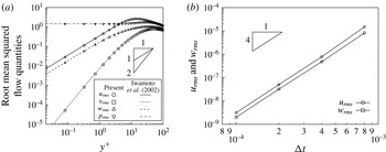
Incompressible wall-bounded channel flow is solved in three dimensions using DNS. This code has been validated in the past (a part of the verification can be found in figure 27(a) in appendix C), and the details of its numerics are described in Hasegawa & Kasagi (Reference Hasegawa and Kasagi2011). The main features and the points specific to this study are summarized below. Periodic boundary conditions are imposed in the streamwise and spanwise directions (see figure 1 for the coordinate system); therefore, the flow is considered to be perfectly homogeneous in these directions. The density and the viscosity are set to be constant, and the friction Reynolds number is set to be
 $Re_{\unicode[STIX]{x1D70F}}=100$
(normalized based on the channel half-height,
 $h$
), corresponding to
 $u^{+}\equiv u_{centreline}/u_{\unicode[STIX]{x1D70F}}\approx 17.$
The flow is observed to be fully developed turbulence, yet with some low Reynolds number characteristics, which are discussed later in § 4.1.
The physical domain size is set to be
 $L_{x}=4\unicode[STIX]{x03C0}h$
,
 $L_{y}=2h$
and
 $L_{z}=4\unicode[STIX]{x03C0}h/3$
to make a fair comparison with Chevalier et al. (Reference Chevalier, Hœpffner, Bewley and Henningson2006), and the
 $3/2$
law is used to remove aliasing errors:
 $L_{x}$
and
 $L_{z}$
are equally spaced with
 $N_{x}=N_{z}=64$
grid points, in which flow quantities are decomposed into
 $42\times 42$
Fourier modes in the streamwise and the spanwise directions, respectively. Unlike their study, however, the Chebyshev collocation method is used in the vertical direction, in which
 $L_{y}$
is discretized into
 $N_{y}=64$
spacings using
 $43$
polynomials. Compared with Chevalier et al. (Reference Chevalier, Hœpffner, Bewley and Henningson2006) using
 $N_{y}=64$
uniform grid spacings with finite differencing, the resolution in
 $y$
is expected to be higher in this study. Thus, the velocity field is spatially differentiated with the spectral methods in all directions.
As opposed to solving the vertical velocity and the wall-normal vorticity, referred to as the
 $v{-}\unicode[STIX]{x1D714}_{y}$
formulation, in many other studies (Kim, Moin & Moser Reference Kim, Moin and Moser1987; Högberg et al.
Reference Högberg, Bewley and Henningson2003; Bewley & Protas Reference Bewley and Protas2004; Chevalier et al.
Reference Chevalier, Hœpffner, Bewley and Henningson2006), primitive variables,
 $u$
,
 $v$
,
 $w$
and
 $p$
, are solved in the current code instead. For pressure decoupling, a fractional step method (Kim & Moin Reference Kim and Moin1985) is used to march the aforementioned transformed velocity field in time: the second-order Adams–Bashforth scheme is adopted for the convection terms and the second-order Crank–Nicholson scheme for the diffusion terms. The time step is set to be
 $\unicode[STIX]{x0394}tu_{\unicode[STIX]{x1D70F}}/h=2.0\times 10^{-3}$
(i.e.
 $\unicode[STIX]{x0394}t^{+}=0.2$
). The solver is used both to solve the original Navier–Stokes equations as well as to run as an observer with the body force defined in § 2.3. The body-force term is inserted before solving the Poisson equation to impose the continuity every time step, as introduced in Suzuki et al. (Reference Suzuki, Ji and Yamamoto2009a
, Reference Suzuki, Ji and Yamamoto2010).
The collocation method allows us to directly compute flow quantities on the wall. On the other hand, we must treat the no-slip boundary condition differently from staggered grid systems. Appendix C describes the details of the no-slip boundary treatment posterior to solving the Poisson equation.
3.2 Sampling statistics
After the flow becomes statistically stationary by running the DNS, we prepare two sets of unsteady flow fields (i.e. true solutions of the original Navier–Stokes equations) for the same conditions but with different initial conditions, plus another extra initial condition. During the first unsteady solution, referred to as the ‘sampling duration’, time-averaged quantities, necessary statistics and correlations are calculated using every time step; at the same time, the wall quantities are recorded also at every time step and the velocity components as well as pressure are recorded at every
 $100$
time steps over all points in the physical space. Likewise, the same unsteady quantities are recorded during the second solution set. To secure enough sampling in the wavenumber space,
 $50\,000$
time steps (i.e.
 $100h/u_{\unicode[STIX]{x1D70F}}$
) are computed for both sets of solutions, and their initial conditions are
 $t=200h/u_{\unicode[STIX]{x1D70F}}$
apart to make these three initial conditions statistically independent. No measurement noise is added to the wall quantities except for the analysis in appendix A.
Using the first solution set the coefficients
 $\boldsymbol{A}$
in (2.8) for the linear stochastic estimation are computed. Assuming that the two sets of solutions are statistically equivalent, these coefficients are commonly applied to the wall measurement for both solutions, and the discrepancies in the velocity field inside the domain from the true solution are compared between the two sets of the solutions. To analyse the observer, the flow is started with the extra initial condition but the second set of the wall measurements is used for the update steps; accordingly, it is monitored if the estimated flow field is sequentially assimilated to the true solution from an unknown initial condition.
Because we decouple wavenumbers in the linear stochastic estimation, the number of samples, 50 000, is much greater than the degrees of freedom, i.e. six in this study. If we were to apply it based on the wall measurement at every grid point in the physical space, the degrees of freedom suddenly expands to
 $64\times 64\times 6=\text{24 576}$
, which is nearly the half of the number of samples. In such a case, linear stochastic estimation can find a linear combination that almost exactly reconstructs the sampled velocity fields up to the degrees of freedom but would not estimate the flow well beyond the sampling duration. Analogous problems occur when the degrees of freedom increase (e.g. by including coupling of the wavenumbers) or when the sampling is limited (e.g. by characterizing the flow with fewer reduced-order models or ensembles); thus, special attention being required for fair evaluation (cf. Chevalier et al.
Reference Chevalier, Hœpffner, Bewley and Henningson2006; Colburn et al.
Reference Colburn, Cessna and Bewley2011).
4 Results and discussion
4.1 Basic flow characteristics at
 $Re_{\unicode[STIX]{x1D70F}}=100$

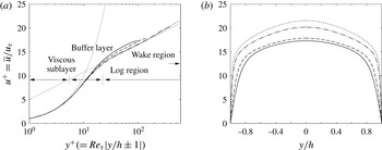
We start with general observations of the flow to be estimated. For reference, we compare flow statistics with the database by Iwamoto, Suzuki & Kasagi (Reference Iwamoto, Suzuki and Kasagi2002), which has been extensively validated in the past. Figure 2 compares the time- and space-averaged streamwise velocity profile, i.e. the time average of
 $\overline{\tilde{u} }(k_{x}=0,y,k_{z}=0)$
, with those at higher Reynolds numbers. All cases collapse very well in the viscous sublayer (
 $y^{+}\lesssim 10$
). Our case,
 $Re_{\unicode[STIX]{x1D70F}}=100$
, indicates a low Reynolds number feature in the log layer, as reported by Moser, Kim & Mansour (Reference Moser, Kim and Mansour1999); namely, the velocity profile in this region overshoots those at high Reynolds numbers, as is expected.
Comparison of the time- and space-averaged streamwise velocity. Line patterns: ——,
 $Re_{\unicode[STIX]{x1D70F}}=100$
in the current study; - - -,
 $Re_{\unicode[STIX]{x1D70F}}=150$
(Iwamoto et al.
Reference Iwamoto, Suzuki and Kasagi2002, and thereafter); – ⋅ – ⋅ –,
 $Re_{\unicode[STIX]{x1D70F}}=396$
;
 $\cdots \cdots$
,
 $Re_{\unicode[STIX]{x1D70F}}=643$
. (a) Profiles near the wall. Thin grey lines indicate
 $u^{+}=y^{+}$
and
 $u^{+}=0.4^{-1}\log y^{+}+5$
. (b) Profiles across the channel.

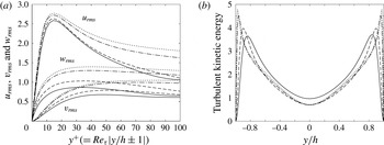
Figure 3 similarly compares velocity fluctuations in our case with those at higher Reynolds numbers. Regardless of
 $Re_{\unicode[STIX]{x1D70F}}$
, the streamwise velocity fluctuation becomes the highest in the buffer layer, in which the linear and the log profiles intersect, and turbulent kinetic energy also forms a peak in this layer. In the physical scale, the peak of turbulent kinetic energy shifts away from the wall with decreasing Reynolds number. Its level near the centreline at
 $Re_{\unicode[STIX]{x1D70F}}=100$
is slightly higher than the other cases, possibly because the aspect ratio of our domain is
 $L_{x}/L_{z}=3$
as opposed to
 $L_{x}/L_{z}=2$
by Iwamoto et al. (Reference Iwamoto, Suzuki and Kasagi2002). It should be noted that we have confirmed the agreement with their database for the same condition in appendix C. In general, our simulation possesses fundamental turbulence characteristics although it indicates some low Reynolds number features.
Now, the correlations of the velocity components,
 $\tilde{u}$
,
 $\tilde{v}$
and
 $\tilde{w}$
, in the flow with the wall measurements,
 $\tilde{\unicode[STIX]{x1D70F}_{x}}$
,
 $\tilde{\unicode[STIX]{x1D70F}_{z}}$
and
 $\tilde{p}$
, are analysed in the wavenumber space. Through these results, the region reconstructible from the instantaneous wall information can be assessed. Four different wavenumber combinations,
 $(k_{x}^{\prime }h,k_{z}^{\prime }h)=(0.5,1.5)$
,
 $(0.5,6)$
,
 $(3,18)$
and
 $(5,30)$
, are analysed for the velocity in the flow; in particular, the second and third combinations are representative of low-/high-speed streaks and quasi-streamwise vortices, respectively, containing a large portion of turbulent kinetic energy and representing key features of near-wall turbulence (Smith & Metzler Reference Smith and Metzler1983; Kim et al.
Reference Kim, Moin and Moser1987). We record the correlation coefficient for each wavenumber combination against each wall quantity over the entire wavenumber space during the sampling duration of
 $100h/u_{\unicode[STIX]{x1D70F}}$
.
Comparison of the fluctuating velocity components (database at higher Reynolds numbers is similarly taken from Iwamoto et al. Reference Iwamoto, Suzuki and Kasagi2002). Line patterns are the same as figure 2. (a) Root mean squares of three velocity components near the wall (a similar figure can be found in Moser et al. Reference Moser, Kim and Mansour1999). (b) Turbulent kinetic energy across the channel.

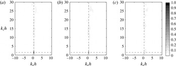
Contours for one of such coefficients, given by
 $$\begin{eqnarray}\text{Cor}[\tilde{u} (k_{x}^{\prime },y,k_{z}^{\prime }),\tilde{\unicode[STIX]{x1D70F}_{x}}(k_{x},y/h=1,k_{z})]\equiv \frac{\left|\overline{\tilde{u} ^{\ast }\left(k_{x}^{\prime },y,k_{z}^{\prime }\right)\tilde{\unicode[STIX]{x1D70F}_{x}}\left(k_{x},1,k_{z}\right)}\right|}{\sqrt{\overline{\left|\tilde{u} \left(k_{x}^{\prime },y,k_{z}^{\prime }\right)\right|^{2}}}\sqrt{\overline{\left|\tilde{\unicode[STIX]{x1D70F}_{x}}\left(k_{x},1,k_{z}\right)\right|^{2}}}},\end{eqnarray}$$
are drawn at three heights in figures 4–6. The overbar above represents the time average over the aforementioned duration: every time step during
 $100h/u_{\unicode[STIX]{x1D70F}}$
is used for the evaluation in the wavenumber space. Here, the lower half-plane (i.e.
 $k_{z}<0$
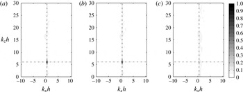
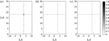
) is omitted because it is complex conjugate of the upper half. Near the wall, a distinctive peak is formed at the same wavenumber as the velocity component. Aside from the peak, weak correlations are found in the vicinity of the same
 $k_{x}$
, indicating spanwise patterns of streamwise vorticity, but mostly less than
 $0.2$
. Although only a single combination (i.e.
 $\tilde{u}$
versus
 $\tilde{\unicode[STIX]{x1D70F}_{x}}$
) is shown here, other correlations across different wavenumbers are also investigated and confirmed to be always low except for the primary peak (i.e. the identical wavenumber). Accordingly, linear stochastic estimation is performed for each wavenumber combination in this study. Moreover, correlation of a velocity component in the flow with a product between two wall quantities should then be further reduced; hence, unlike unsteady laminar flows, the justification of nonlinear stochastic estimation is weak for such turbulent flows.
Correlation coefficients of
 $\tilde{u} (k_{x}^{\prime }h=0.5,y,k_{z}^{\prime }h=1.5)$
with
 $\tilde{\unicode[STIX]{x1D70F}}_{x}(k_{x},y/h=1,k_{z})$
. (a)
 $y/h=0.942$
(peak correlation
 $0.978$
at the same wavenumber point indicated by broken lines). (b)
 $y/h=0.803$
(
 $0.614$
). (c)
 $y/h=0$
(
 $0.129$
at a different wavenumber point).

Correlation coefficients of
 $\tilde{u} (k_{x}^{\prime }h=0.5,y,k_{z}^{\prime }h=6.0)$
with
 $\tilde{\unicode[STIX]{x1D70F}}_{x}(k_{x},y/h=1,k_{z})$
. (a)
 $y/h=0.942$
(peak correlation
 $0.991$
at the same wavenumber point indicated by broken lines). (b)
 $y/h=0.803$
(
 $0.902$
). (c)
 $y/h=0$
(
 $0.154$
at a different wavenumber point).

Correlation coefficients of
 $\tilde{u} (k_{x}^{\prime }h=3.0,y,k_{z}^{\prime }h=18.0)$
with
 $\tilde{\unicode[STIX]{x1D70F}}_{x}(k_{x},y/h=1,k_{z})$
. (a)
 $y/h=0.942$
(peak correlation
 $0.776$
at the same wavenumber point indicated by broken lines). (b)
 $y/h=0.803$
(
 $0.120$
). (c)
 $y/h=0$
(
 $0.101$
at a different wavenumber point).

By focusing on the same wavenumber between
 $\tilde{\unicode[STIX]{x1D70F}_{x}}$
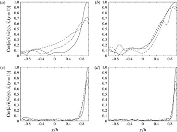
on the wall and the velocity components, the correlation coefficients are plotted across the channel in figure 7. At low wavenumbers, i.e.
 $(k_{x}h,k_{z}h)=(0.5,1.5)$
and
 $(0.5,6.0)$
, high correlation is retained beyond the viscous sublayer (
 $y/h\lesssim 0.8$
), but all three correlations decay toward the centreline. At higher wavenumbers, the correlations sharply drop beyond the viscous sublayer. At all wavenumbers, the streamwise velocity correlation is appreciably higher than the other two components, indicating that the streamwise shear-stress measurement is effective to estimate the streamwise velocity component.
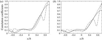
Figure 8 similarly plots the correlations of
 $\tilde{\unicode[STIX]{x1D70F}_{z}}$
and
 $\tilde{p}$
at
 $(k_{x}h,k_{z}h)=(0.5,6.0)$
. In contrast to the correlation with
 $\tilde{\unicode[STIX]{x1D70F}_{x}}$
above, these two wall quantities,
 $\tilde{\unicode[STIX]{x1D70F}_{z}}$
and
 $\tilde{p}$
, are primarily responsible for
 $\tilde{w}$
and
 $\tilde{v}$
(these trends are more or less similar at other wavenumbers, not shown). The correlation with
 $\tilde{p}$
is lower than those with
 $\tilde{\unicode[STIX]{x1D70F}_{x}}$
and
 $\tilde{\unicode[STIX]{x1D70F}_{z}}$
; namely, the pressure signal is less effective than the shear stresses. We can confirm this by applying linear stochastic estimation with individual components (the results are not shown). Regardless of the combinations, all the profiles decay as low as
 $0.2$
at the centreline. These results imply inherent difficulty with instantaneous estimation near the centreline based on the wall measurements.
Correlation coefficients of
 $\tilde{\unicode[STIX]{x1D70F}_{x}}(y/h=1)$
with three velocity components at the same wavenumber. Line patterns: ——, with
 $\tilde{u}$
; - - -, with
 $\tilde{v}$
; – ⋅ – ⋅ –, with
 $\tilde{w}$
. (a)
 $(k_{x}h,k_{z}h)=(0.5,1.5)$
. (b)
 $(0.5,6.0)$
. (c)
 $(3.0,18.0)$
. (d)
 $(5.0,30.0)$
.

At low wavenumbers, we find discernible correlation recovery on the opposite side of the wall (i.e.
 $y/h=-1$
) in figures 7(a–b) and 8. We attribute this phenomenon to large-scale motions across the channel represented by lower-order Chebyshev polynomials. This motivates us to process wall quantities on both sides simultaneously in the stochastic estimation. By expanding the degrees of freedom only from three to six, we can appreciably improve the accuracy of estimation (comparison not shown).
Correlation coefficients of the other wall quantities with three velocity components at
 $(k_{x}h,k_{z}h)=(0.5,6.0)$
. Line patterns are the same as figure 7. (a)
 $\tilde{\unicode[STIX]{x1D70F}_{z}}(y/h=1)$
. (b)
 $\tilde{p}(y/h=1)$
.

4.2 Instantaneous estimation: linear stochastic estimation
Next, we discuss the results of instantaneous velocity estimate using the linear stochastic estimation explained in § 2.2. To make the comparison of our results with those by Chevalier et al. (Reference Chevalier, Hœpffner, Bewley and Henningson2006) easier, we define the correlation coefficient in the same manner:
 $$\begin{eqnarray}\text{Cor}\left(u_{LSE}^{\prime },u_{DNS}^{\prime }\right)\equiv \frac{\displaystyle \left|\overline{\int _{0}^{L_{x}}\int _{0}^{L_{z}}u_{LSE}^{\ast ^{\prime }}u_{DNS}^{\prime }\,\text{d}x\,\text{d}z}\right|}{\displaystyle \sqrt{\overline{\int _{0}^{L_{x}}\int _{0}^{L_{z}}\left|u_{LSE}^{\prime }\right|^{2}\,\text{d}x\,\text{d}z}}\sqrt{\overline{\int _{0}^{L_{x}}\int _{0}^{L_{z}}\left|u_{DNS}^{\prime }\right|^{2}\,\text{d}x\,\text{d}z}}},\end{eqnarray}$$
where
 $u_{LSE}^{\prime }$
and
 $u_{DNS}^{\prime }$
denote the streamwise velocity fluctuation based on the linear stochastic estimation and that of the true solution from the original DNS, respectively. Here, the overbar represents time average over the
 $100h/u_{\unicode[STIX]{x1D70F}}$
period but takes a sample every
 $100$
time steps for physical quantities, a total being
 $500$
samples. We similarly define the correlation coefficients for the other velocity components,
 $v^{\prime }$
and
 $w^{\prime }$
, as well as the Reynolds stresses,
 $u^{\prime }v^{\prime }$
,
 $v^{\prime }w^{\prime }$
and
 $w^{\prime }u^{\prime }$
.
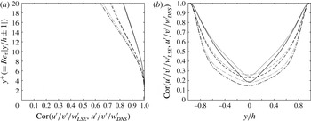
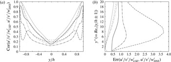
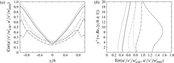
Figure 9(a) shows the correlation coefficients of the three velocity components near the wall. Here, we plot the estimates for the two sets mentioned in § 3.2: (i) the first set during which statistics for the linear stochastic estimation are taken (thin grey lines) and (ii) the second set sufficiently after the sampling duration (thick black lines). In
 $y^{+}\leqslant 20$
, the correlations between the two sets are nearly the same. These profiles also agree very well with those of the extended Kalman filter by Chevalier et al. (Reference Chevalier, Hœpffner, Bewley and Henningson2006) in figure 6 of their paper. To be precise, our streamwise velocity correlation tends to be slightly lower than theirs, while the vertical and spanwise velocity correlations are somewhat better.
Correlation coefficients of velocity fluctuations. Line patterns: ——,
 $\text{Cor}(u_{LSE}^{\prime },u_{DNS}^{\prime })$
; – – –,
 $\text{Cor}(v_{LSE}^{\prime },v_{DNS}^{\prime })$
; – ⋅ – ⋅ –,
 $\text{Cor}(w_{LSE}^{\prime },w_{DNS}^{\prime })$
. Thick black lines indicate the estimates sufficiently after the sampling duration, and thin grey lines those during the sampling duration. (a) Profiles near the wall. (b) Profiles across the channel.

Figure 9(b) reveals that all the correlations drop toward the centreline. In particular, the correlations after the sampling duration are clearly lower than those during the sampling duration beyond the viscous sublayer (
 $|y/h|\lesssim 0.8$
). This implies that the statistics between the two periods, although
 $100h/u_{\unicode[STIX]{x1D70F}}$
apart, are not exactly equivalent, and the linear stochastic estimation ‘memorizes’ a part of flow patterns rather than takes statistical correlation. Interestingly, the streamwise velocity generally gives the highest correlation except near the centreline for the result outside the sampling duration. The estimation of spanwise velocity fluctuations is least successful over the entire channel.
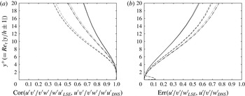
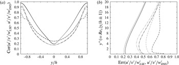
We also plot other quantities evaluated by Chevalier et al. (Reference Chevalier, Hœpffner, Bewley and Henningson2006). The correlation profiles of all the Reynolds stresses in figure 10(a) are again very close to their results (see figure 8 in Chevalier et al.
Reference Chevalier, Hœpffner, Bewley and Henningson2006). Not surprisingly,
 $\text{Cor}(v^{\prime }w_{LSE}^{\prime },v^{\prime }w_{DNS}^{\prime })$
yields the lowest correlation because the individual estimates of
 $v^{\prime }$
and
 $w^{\prime }$
are worse than
 $u^{\prime }$
.
Profiles of other quantities near the wall. Distinction between the thick and thin lines is the same as figure 9. (a) Reynolds stresses. Line patterns: ——,
 $\text{Cor}(u^{\prime }v_{LSE}^{\prime },u^{\prime }v_{DNS}^{\prime })$
; – – –,
 $\text{Cor}(v^{\prime }w_{LSE}^{\prime },v^{\prime }w_{DNS}^{\prime })$
; – ⋅ – ⋅ –,
 $\text{Cor}(w^{\prime }u_{LSE}^{\prime },w^{\prime }u_{DNS}^{\prime })$
. (b) Errors defined in (4.3). Line patterns: ——,
 $\text{Err}(u_{LSE}^{\prime },u_{DNS}^{\prime })$
; – – –,
 $\text{Err}(v_{LSE}^{\prime },v_{DNS}^{\prime })$
; – ⋅ – ⋅ –,
 $\text{Err}(w_{LSE}^{\prime },w_{DNS}^{\prime })$
.

In addition, the normalized error is defined as
 $$\begin{eqnarray}\text{Err}(u_{LSE}^{\prime },u_{DNS}^{\prime })\equiv \frac{\displaystyle \sqrt{\overline{\int _{0}^{L_{x}}\int _{0}^{L_{z}}\left|u_{LSE}^{\prime }-u_{DNS}^{\prime }\right|^{2}\,\text{d}x\,\text{d}z}}}{\displaystyle \sqrt{\overline{\int _{0}^{L_{x}}\int _{0}^{L_{z}}\left|u_{DNS}^{\prime }\right|^{2}\,\text{d}x\,\text{d}z}}},\end{eqnarray}$$
for the streamwise velocity fluctuation and the other velocity components are similarly defined. The results of these errors in figure 10(b) are consistent with figure 9(a) in the sense that the agreement is similar to Chevalier et al. (Reference Chevalier, Hœpffner, Bewley and Henningson2006). To be precise, our estimate of
 $u^{\prime }$
deviates slightly more for greater
 $y^{+}$
, while our other two components give better estimates than theirs. Because we impose no measurement noise, the errors almost vanish near the wall except in the very small
 $v^{\prime }$
region. The differences due to the sampling duration are again relatively small, and we analyse the data only after the sampling duration (i.e. the second set) in the rest of the discussion.
These results consistently suggest that if we can remove the measurement noise, the linear stochastic estimation can essentially estimate velocity fields as good as the extended Kalman filter. Both approaches take the same information from the wall, but the major difference is that the former one estimates the velocity field from instantaneous information while the latter one optimizes the forcing distribution and accounts for the dynamics in the course of time. General expectation is the observer solving the Navier–Stokes equations compensates the information propagating from the wall. However, the fact that the agreement away from the wall is comparable between the two approaches may imply that the extended Kalman filter only suppresses the measurement noise and hardly contributes to improvement of the estimation beyond the viscous sublayer.
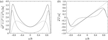
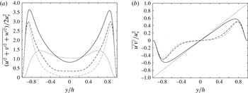
Profiles of turbulent quantities across the channel. Line patterns: ——, original Navier–Stokes; – – –, linear stochastic estimation. (a) Turbulent kinetic energy (
 $\cdots \cdots$
, the squared difference). (b) Reynolds shear stress (
 $\cdots \cdots$
, total shear stress).

We elucidate the reason for poor estimates away from the wall. Figure 11(a) compares the turbulent kinetic energy profile of the linear stochastic estimation with that of the true solution together with their squared difference. We notice that the turbulence intensity in the linear stochastic estimation diminishes beyond the buffer layer. When the correlation between the wall quantity and the velocity in the flow drops, as seen in § 4.1, the magnitude of the coefficients in (2.6) decreases. Namely, if the estimation is less certain, the linear stochastic estimation produces smaller values to minimize errors, resulting in over-suppression of turbulent motion, especially in the log layer. Likewise, figure 11(b) reveals that the contribution of the
 $\overline{u^{\prime }v^{\prime }}$
shear-stress component is much lower in the linear stochastic estimation near the centreline. On the other hand, the mean streamwise velocity profile is invariant since we determine the linear coefficients
 $\boldsymbol{a}^{\dagger }$
in (2.5) relative to the mean flow; namely, the shear stress by the molecular viscosity remains the same between the true solution and the linear stochastic estimation.
In this sense, the correlation coefficient is somewhat misleading since
 $\int \int |u_{LSE}^{\prime }|^{2}\,\text{d}x\text{d}z$
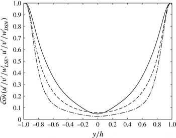
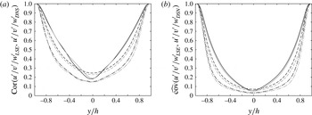
in the denominator of (4.2) diminishes toward the centreline, elevating its value. It is rather intuitive if we plot the covariance normalized by the auto-correlation as
 $$\begin{eqnarray}\widehat{\text{cov}}\left(u_{LSE}^{\prime },u_{DNS}^{\prime }\right)\equiv \text{Cov}\left(u_{LSE}^{\prime },u_{DNS}^{\prime }\right)/\text{Cov}\left(u_{DNS}^{\prime },u_{DNS}^{\prime }\right)=\frac{\displaystyle \left|\overline{\int _{0}^{L_{x}}\int _{0}^{L_{z}}u_{LSE}^{\ast ^{\prime }}u_{DNS}^{\prime }\,\text{d}x\,\text{d}z}\right|}{\displaystyle \overline{\int _{0}^{L_{x}}\int _{0}^{L_{z}}\left|u_{DNS}^{\prime }\right|^{2}\,\text{d}x\,\text{d}z}}.\end{eqnarray}$$
Figure 12 now reveals that the estimation is mostly unsuccessful away from the wall and indicates the limitation of instantaneous measurement based on the wall quantities. Since both correlation coefficients and normalized errors in Chevalier et al. (Reference Chevalier, Hœpffner, Bewley and Henningson2006) essentially show the same profiles as our profiles, their estimation must have the common problem. The key for further improvement is to infer motions away from the wall, especially beyond the peaks of turbulent kinetic energy.
Normalized covariance given by (4.4). Line patterns: ——,
 $\widehat{\text{cov}}(u_{LSE}^{\prime },u_{DNS}^{\prime })$
; - - -,
 $\widehat{\text{cov}}(v_{LSE}^{\prime },v_{DNS}^{\prime })$
; – ⋅ – ⋅ –,
 $\widehat{\text{cov}}(w_{LSE}^{\prime },w_{DNS}^{\prime })$
.

We subsequently visualize the discrepancy in the wavenumber space. To measure the success of the estimation, we similarly define the normalized covariance between the linear stochastic estimation and the true solution for each
 $(k_{x},k_{z})$
:
 $$\begin{eqnarray}\displaystyle \widehat{\text{cov}}\left[\tilde{u} _{LSE}\left(k_{x},y,k_{z}\right),\tilde{u} _{DNS}\left(k_{x},y,k_{z}\right)\right] & \equiv & \displaystyle \text{Cov}\left(\tilde{u} _{LSE},\tilde{u} _{DNS}\right)/\text{Cov}\left(\tilde{u} _{DNS},\tilde{u} _{DNS}\right)\nonumber\\ \displaystyle & = & \displaystyle \frac{\left|\overline{\tilde{u} _{LSE}^{\ast }\left(k_{x},y,k_{z}\right)\tilde{u} _{DNS}\left(k_{x},y,k_{z}\right)}\right|}{\overline{\left|\tilde{u} _{DNS}\left(k_{x},y,k_{z}\right)\right|^{2}}},\end{eqnarray}$$
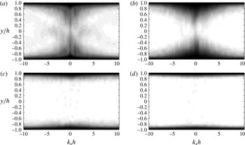
where the time average again takes every time step for wavenumber components. Figure 13 draws its contours for
 $\tilde{u}$
on selected constant
 $k_{z}$
planes corresponding to figure 7. Regardless of the wavenumbers, the normalized covariance reaches approximately unity near the wall: its thickness decreases with increasing
 $k_{z}$
. In the vicinity of the centreline (i.e.
 $y=0$
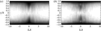
), the covariance is high only at low wavenumbers. We also display the contours for
 $\tilde{v}$
and
 $\tilde{w}$
on
 $k_{z}h=6.0$
in figure 14, showing the same trends. Thus, the stochastic estimation can reconstruct only very large motions, and its capability rapidly deteriorates from the buffer layer with increasing wavenumber.
Contours of normalized covariance for
 $\tilde{u}$
given by (4.5). The domain extends over the entire
 $k_{x}-y$
space. (a)
 $k_{z}h=1.5$
. (b)
 $k_{z}h=6.0$
. (c)
 $k_{z}h=18.0$
. (d)
 $k_{z}h=30.0$
.

Contours of normalized covariance at
 $k_{z}h=6.0$
. (a) for
 $\tilde{v}$
. (b) for
 $\tilde{w}$
.

In contrast to the turbulence estimation based on the wall measurement, Baars, Hutchins & Marusic (Reference Baars, Hutchins and Marusic2016) reported success in estimation of near-wall turbulent statistics from large-scale motions in the log layer and beyond. By extracting coherent motions from pointwise measurement in the log layer, they conversely infer streamwise velocity fluctuations beneath it using linear stochastic estimation even at higher Reynolds numbers (i.e.
 $Re_{\unicode[STIX]{x1D70F}}>O(10^{3})$
). On the other hand, their study also reveals the limitation of the instantaneous estimation in the buffer layer, in which incoherent motions dominate the peak of the energy spectrum. This is consistent with our observation below that it is difficult to infer instantaneous motions in the log layer from those in the viscous sublayer.
4.3 State observer combined with the linear stochastic estimation
Finally, an observer is established by imposing the body-force term in the Navier–Stokes equations, as explained in § 2.3. In this approach, a part of the estimation is given instantaneously by the linear stochastic estimation, while the rest is advanced from the previous time step using the DNS. Therefore, it is expected that the over-suppression of turbulent kinetic energy found in the previous section can be relaxed by propagating the information toward the centreline from the wall. Through this process, the pressure field is simultaneously produced, which is also evaluated below.
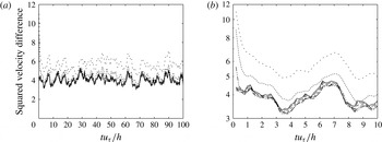
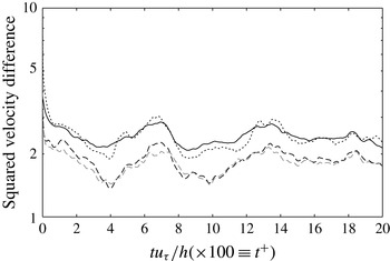
Time histories of the squared velocity difference given by (4.6). Line patterns:
 $\cdot \,\cdot \,\cdot \,\cdot \,\cdot$
,
 $\unicode[STIX]{x1D716}=1$
;
 $\cdots \cdots$
,
 $\unicode[STIX]{x1D716}=2$
;
 $-\cdot \cdot -\cdot \cdot -$
,
 $\unicode[STIX]{x1D716}=5$
; – ⋅ – ⋅ –,
 $\unicode[STIX]{x1D716}=10$
; – – –,
 $\unicode[STIX]{x1D716}=20$
;— —,
 $\unicode[STIX]{x1D716}=50$
; ——, linear stochastic estimation. (a) Linear scale over the entire sampling duration. (b) Log scale in the initial part.

When the errors in the forcing term are uncorrelated in space, and its magnitude is uniform, we can apply the criterion in Suzuki et al. (Reference Suzuki, Ji and Yamamoto2009a
) for the weight of the forcing,
 $\unicode[STIX]{x1D716}$
, in (2.13). In such a case,
 $\unicode[STIX]{x1D716}$
must overcome the maximum amplification rate of the system (in the current flow, the system is linearly stable; hence, it is difficult to directly determine the threshold). However, the errors are partially correlated in space, and the accuracy of the linear stochastic estimation is significantly deteriorated outside the viscous sublayer. Thus, several constant weights are examined below. In figure 15, time histories of the squared velocity difference given below are plotted for various
 $\unicode[STIX]{x1D716}$
:
 $$\begin{eqnarray}\displaystyle \frac{1}{L_{x}L_{z}}\int _{0}^{L_{x}}\!\int _{-h}^{h}\!\int _{0}^{L_{z}}\!\left(u_{Obs}-u_{DNS}\right)^{2}+\left(v_{Obs}-v_{DNS}\right)^{2}+\left(w_{Obs}-w_{DNS}\right)^{2}\,\text{d}x\,\text{d}y\,\text{d}z. & & \displaystyle\end{eqnarray}$$
Here, the subscript
 $\text{Obs}$
denotes a quantity from the observer, which is equivalent to that with a hat mark in (2.13). Since we impose the initial condition inconsistent with the wall information for the rest of the time, the discrepancy starts with the maximum value and soon becomes stationary for all the cases. This shows a sequential data assimilation feature, but the observer can suppress the discrepancy by approximately one third at best. The least weight yields the slowest initial convergence, and the slope becomes steeper with increasing
 $\unicode[STIX]{x1D716}$
. We should note that the least weight here,
 $\unicode[STIX]{x1D716}=1$
, is still strong in general control applications, and the magnitude of
 $\unicode[STIX]{x1D716}=O(10)$
is actually necessary to reduce the errors to the level equivalent to the linear stochastic estimation. This approximately corresponds to the frequency of streamwise-vortex passages above the wall. To remove the initial transient states, we take statistics from
 $t=10h/u_{\unicode[STIX]{x1D70F}}$
in the following discussion.
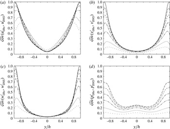
Normalized covariance given by the observer with different weights. Line patterns:
 $\cdot \,\cdot \,\cdot \,\cdot \,\cdot$
,
 $\unicode[STIX]{x1D716}=1$
;
 $\cdots \cdots$
,
 $\unicode[STIX]{x1D716}=2$
;
 $-\cdot \cdot -\cdot \cdot -$
,
 $\unicode[STIX]{x1D716}=5$
; – ⋅ – ⋅ –,
 $\unicode[STIX]{x1D716}=10$
; – – –,
 $\unicode[STIX]{x1D716}=20$
;— —,
 $\unicode[STIX]{x1D716}=50$
; ——, linear stochastic estimation. (a)
 $\widehat{\text{cov}}(u_{Obs}^{\prime },u_{DNS}^{\prime })$
. (b)
 $\widehat{\text{cov}}(v_{Obs}^{\prime },v_{DNS}^{\prime })$
. (c)
 $\widehat{\text{cov}}(w_{Obs}^{\prime },w_{DNS}^{\prime })$
. (d)
 $\widehat{\text{cov}}(p_{Obs}^{\prime },p_{DNS}^{\prime })$
. No linear stochastic estimation available for pressure.

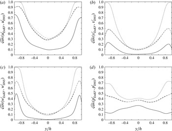
Subsequently, we compare the normalized velocity covariances given in (4.4) for various
 $\unicode[STIX]{x1D716}$
in figure 16(a–c). To achieve good agreement near the wall, we find that very strong forcing is necessary, especially for
 $v$
and
 $w$
. The magnitude of the velocity fluctuations in the viscous sublayer is much smaller than that near the peak of turbulent kinetic energy, as shown in figure 11. In the observer, strong motions in the buffer layer, which are inaccurately estimated from the wall information, evolve over time and dominate over weak fluctuations near the wall, which are accurately imposed by the linear stochastic estimation. Thus, we must force the right hand side strongly enough to overcome it and to retain accurate motions near the wall.
Away from the wall, on the other hand, smaller weights can improve estimate. For the streamwise velocity in figure 16(a),
 $\unicode[STIX]{x1D716}=1$
gives the highest covariance in
 $|y/h|\lesssim 0.4$
(this will be clear in figure 17), and the covariance degrades with increasing weight in this region. Likewise,
 $\unicode[STIX]{x1D716}=5$
provides the highest covariance for the spanwise velocity over a wide range of
 $y$
in figure 16(c), while the linear stochastic estimation predicts best across the entire channel for the vertical velocity in figure 16(b). If we compare the correlation coefficients instead (not shown), the best weight changes, but the trend of better estimation with a smaller weight away from the wall is more or less similar. By relaxing the forcing, we can improve the over-suppression of turbulent kinetic energy in the log layer, and this benefit seems to surpass the influence of strong motions inaccurately estimated in the buffer layer.
Regarding the estimated pressure field, the normalized covariance monotonically improves with increasing
 $\unicode[STIX]{x1D716}$
, as shown in figure 16(d). Because of the nature of the wall boundary condition, i.e.
 $\unicode[STIX]{x2202}p/\unicode[STIX]{x2202}y\approx 0$
, pressure exerted by the motions in the buffer layer penetrates the viscous sublayer. As a result, the pressure estimation on the wall is less successful compared with that of velocity fluctuations. On the other hand, such large-scale motions partly influence pressure near the centreline, leading to better estimates than those of velocity fluctuations.
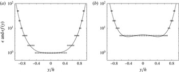
The weight of the forcing
 $\unicode[STIX]{x1D716}$
providing the best covariance at each
 $y$
(denoted by ○) and a quartic function best fitting to them (denoted by a solid line), which is used as the spatially varying
 $\unicode[STIX]{x1D716}f(y)$
(
 $\text{max}[\unicode[STIX]{x1D716}]\equiv 100$
). (a) For streamwise velocity. (b) For spanwise velocity.

Referring to figure 16, we eventually show that the normalized covariance can be improved by varying
 $\unicode[STIX]{x1D716}$
as a function of
 $y$
. As a simple example, figure 17 plots the weight
 $\unicode[STIX]{x1D716}$
that provides the best normalized covariance in figure 16 at each
 $y$
(points at which the linear stochastic estimation gives the best covariance are eliminated). We then fit a quartic function to those points assuming symmetry and introduce such spatially varying
 $\unicode[STIX]{x1D716}f(y)$
(
 ${\leqslant}100$
is imposed) into the observer for the streamwise and spanwise velocity components. For the vertical velocity estimation, the linear stochastic estimation always yields the best covariance; hence, we impose constant
 $\unicode[STIX]{x1D716}=100$
across the channel for simplicity (a plot for
 $v^{\prime }$
is omitted in figure 17).
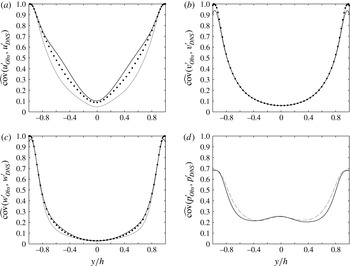
Normalized covariance of the observer with the spatially varying
 $\unicode[STIX]{x1D716}f(y)$
given in figure 17 (denoted by a thicker black line). For reference, the envelope of the best estimate in figure 16 is plotted by dots together with the linear stochastic estimation by a thin grey line for (a–c). (a)
 $\widehat{\text{cov}}(u_{Obs}^{\prime },u_{DNS}^{\prime })$
. (b)
 $\widehat{\text{cov}}(v_{Obs}^{\prime },v_{DNS}^{\prime })$
. (c)
 $\widehat{\text{cov}}(w_{Obs}^{\prime },w_{DNS}^{\prime })$
. (d)
 $\widehat{\text{cov}}(p_{Obs}^{\prime },p_{DNS}^{\prime })$
. No linear stochastic estimation available, but the
 $\unicode[STIX]{x1D716}=50$
case from figure 16(d) is plotted by a grey dashed line for reference.

In figure 18, we compare the results for the set of such
 $\unicode[STIX]{x1D716}f(y)$
with the envelopes of the best estimate in figure 16 as well as the linear stochastic estimation. Since a result of the linear stochastic estimation is unavailable for the pressure estimation, we overlay the
 $\unicode[STIX]{x1D716}=50$
case for reference in figure 18(d). The spatially varying weight predicts the streamwise and spanwise velocity components better than the other two profiles except very close to the wall. In particular, the improvement for
 $\widehat{\text{cov}}(u_{Obs}^{\prime },u_{DNS}^{\prime })$
is appreciable over a wide range of
 $y$
. In contrast, the covariance for the vertical velocity approximately remains the same since we only impose strong uniform forcing across the channel. Likewise, the degree of success in the pressure estimation is similar to the strongest uniform forcing of
 $\unicode[STIX]{x1D716}=50$
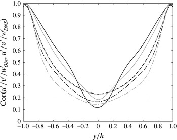
. Although we have not fully optimized the weight, these results demonstrate that we can improve the estimate in a certain degree by tuning the forcing function. On the other hand, the improvement of estimation for the two velocity components hardly helps the improvement of the remaining components. The comparison of the correlation coefficients in figure 19 shows consistent results.
Comparison of the correlation coefficients. Line patterns: ——,
 $\text{Cor}(u_{Obs}^{\prime },u_{DNS}^{\prime })$
; – – –,
 $\text{Cor}(v_{Obs}^{\prime },v_{DNS}^{\prime })$
; – ⋅ – ⋅ –,
 $\text{Cor}(w_{Obs}^{\prime },w_{DNS}^{\prime })$
. Thick black lines denote the results of the spatially varying
 $\unicode[STIX]{x1D716}f(y)$
and thin grey lines those of the linear stochastic estimation.

It is evident from figure 20(a) that the spatially varying weight helps relax the over-suppression of turbulent kinetic energy away from the wall compared with the linear stochastic estimation. However, the errors themselves somewhat increase near the centreline, indicating that the elevated turbulence intensity does not accurately fill large-scale motions. Figure 20(b) clarifies that the shear stress also slightly increases beyond the buffer layer. Unlike the linear stochastic estimation, the sum of the molecular and the eddy viscosities must comprise the total shear stress, which dictates the mean velocity profile. As a result,
 $\overline{u}(y)$
in the observer slightly deviates from the true solution. Nonetheless, the spatially varying weight provides the best estimate in the most regions for the streamwise and spanwise velocity components. Although we may speculate improvement by further relaxation of the forcing or by further enhancement of turbulent kinetic energy near the centreline, we found no other effective profile of
 $\unicode[STIX]{x1D716}f(y)$
among many other trials.
Turbulent quantities generated by the spatially varying weight. Line patterns: ——, original Navier–Stokes; – – – (black), spatially varying
 $\unicode[STIX]{x1D716}f(y)$
; – – – (thin grey), linear stochastic estimation. (a) Turbulent kinetic energy (
 $\cdots \cdots$
, the squared difference). (b) Reynolds shear stress (
 $\cdots \cdots$
, total shear stress).

Comparison of instantaneous flow fields in a three-dimensional view. Iso-surfaces of the second invariant of the velocity gradient tensor
 $\unicode[STIX]{x1D64C}_{+}$
are displayed to visualize vortex cores. Contours of the streamwise velocity are also drawn. (a) True solution on the top (
 $\unicode[STIX]{x1D64C}_{+}=-0.02$
). (b) Estimate using the spatially varying weight on the bottom (
 $\unicode[STIX]{x1D64C}_{+}=-0.01$
).

Comparison of instantaneous flow fields in a cross-sectional view at
 $x/h=3.0$
. Streamwise velocity contours are drawn with velocity vectors on perpendicular planes. (a) True solution. (b) Estimate using the spatially varying weight.

In figure 21, an instantaneous flow field estimated using the spatially varying weight is compared with the true solution at one of the best instants in a three-dimensional view. Their cross-sections are also compared in figure 22. Although large-scale streaks creeping near the wall are estimated relatively well, those detached from the wall as well as quasi-streamwise vortices away from the wall are mostly smeared, as expected from the results above. It is rather surprising from figure 22 that such distinctive structures are still difficult to be reconstructed based on the wall measurement with the full resolution. We should remember, however, that any linear combinations of the flow representation cannot improve the estimation, and the weak correlation across different wavenumbers would make nonlinear estimation ineffective.
In appendix D, we apply the ensemble Kalman filter (Evensen Reference Evensen1994) analogous to the work by Colburn et al. (Reference Colburn, Cessna and Bewley2011) to the current channel geometry. Although there are some differences in the flow solver architecture, we examine a few possible scenarios to replicate their work. Counter to their conclusion, the correlations near the centreline are less than
 $0.5$
for all the cases (our results are displayed based on the normalized covariance, but this statement still holds). This is rather consistent with our analyses above. Thus, our results imply that the observer solving the dynamical system improves the accuracy in the viscous sublayer in a limited extent relative to the instantaneous estimation, i.e. the linear stochastic estimation. Although Chevalier et al. (Reference Chevalier, Hœpffner, Bewley and Henningson2006) reported comparable results using the extended Kalman filter in
 $y^{+}\leqslant 20$
, it is fair from the discussions in appendices to ascribe the major contribution of the estimation in this region to the instantaneous estimation rather than the observer solving the dynamical system or the optimized feedback.
We observe that a series of our analyses reveal generic viewpoints in turbulent flow estimation based on wall measurement. The results of the following two analyses indicate that the linear part of the stochastic estimation, which is decoupled in the wavenumber space, dictates instantaneous estimation: one is poor correlation across different wavenumbers between the quantities on the wall and the velocity components in the flow, as shown in § 4.1; the other is limited improvement in the estimation by including time derivatives of the measured quantities and by using the ensemble Kalman filter, performed in appendices B and D, respectively. In addition, the analysis in § 2.2 manifests that the results of the estimation should be independent of the flow representation. Therefore, we cannot expect much improvement by incorporating nonlinearity or temporal variation in the estimation scheme or by changing it from the wavenumber space to the physical space except that they may help ‘memorize’ flow patterns during the sampling duration. The linear stochastic estimation can accurately reconstruct velocity components in the viscous sublayer, but inaccurately estimated motions in the buffer layer inevitably disrupt the estimation toward the centreline. Even by introducing an observer that solves the full Navier–Stokes equations, we can improve the estimation in a limited extent beyond the viscous sublayer. All these results may imply inherent difficulty of turbulent flow estimation even using sequential data assimilation techniques. Such techniques can remove unbiased uncorrelated measurement noise, but even a simple sequential observer has the same function, as demonstrated in appendix A. In fact, the accuracy of the estimation by using the extended Kalman filter (Chevalier et al. Reference Chevalier, Hœpffner, Bewley and Henningson2006) is only as good as the linear stochastic estimation. There is a study reporting nearly perfect estimation of a similar turbulent channel flow based on analogous wall measurements using the ensemble Kalman filter (Colburn et al. Reference Colburn, Cessna and Bewley2011). However, which function of their method truly enables the success is not understood.
5 Conclusions
We have tackled turbulent flow estimation based on the wall measurement by solving a channel flow with periodic boundary conditions at
 $Re_{\unicode[STIX]{x1D70F}}=100$
with DNS. By introducing linear stochastic estimation, we instantaneously estimate velocity fields from the two wall shear-stress components and the pressure fluctuation over the entire wavenumber space. Subsequently, we have used it to develop a simple observer; namely, a nonlinear dynamical system is solved with DNS to propagate the state vector consisting of velocity components, and it is sequentially updated by the body-force term given by the linear stochastic estimation. Degrees of success have been measured based on the normalized covariance as well as the correlation coefficients and the normalized errors, as reported by Chevalier et al. (Reference Chevalier, Hœpffner, Bewley and Henningson2006). The correlations between the three quantities measured on the wall and the velocity components inside the channel have also been evaluated in the wavenumber space. To support our claim, the ensemble Kalman filter has been performed by following the study by Colburn et al. (Reference Colburn, Cessna and Bewley2011). In addition, the effect of the uncorrelated white noise and the improvement by including time derivatives of the wall measurement have been analysed.
The linear stochastic estimation perfectly reconstructs all three velocity components right above the wall; however, the correlation coefficients significantly decay toward the centreline as low as
 $0.3$
or less. We can also estimate the Reynolds stresses comparably well, but the correlation coefficients diminish even more steeply. The bottleneck of the stochastic estimation is over-suppression of the velocity fluctuations beyond the viscous sublayer: because stochastic estimation determines a flow quantity by minimizing the least-squares difference, it tends to underestimate values in highly uncertain regions. In turn, the correlation coefficient may under-emphasize the discrepancy from the true solution due to the corresponding decrease in the denominator; hence, we have introduced the normalized covariance as a relevant measure.
We have investigated the effects of forcing strength in the observer. To achieve the accuracy comparable to the linear stochastic estimation near the wall, we must set the right-hand side of the Navier–Stokes equations to ten times the velocity difference or greater (i.e.
 $\unicode[STIX]{x1D716}\gtrsim 10$
). Strong feedback gain is necessary for weak fluctuations in the viscous sublayer, which are accurately estimated, to overcome strong motions in the buffer layer, which are inaccurately estimated. On the other hand, strong uniform forcing hardly alleviates over-suppression of turbulent kinetic energy near the centreline. In fact, our results show that weaker forcing improves the estimation in the log layer for the streamwise and spanwise velocity components. This motivates us to examine a spatially varying weight on the forcing which takes the maximum near the wall and diminishes away from it; as a result, the normalized covariances for those two velocity components become somewhat higher in the log layer than any of the uniform forcing weights.
Chevalier et al. (Reference Chevalier, Hœpffner, Bewley and Henningson2006) applied the extended Kalman filter to the same problem but including uncorrelated white noise in the measured quantities. The accuracy of their velocity estimation in
 $y^{+}\lesssim 20$
is indeed almost the same as our result of the linear stochastic estimation without noise. On the other hand, we have uncovered that a simple sequential processing can essentially remove uncorrelated noise. Assuming that the sequential process in the Kalman filter suppresses the measurement noise in their study, our study indicates that the instantaneous estimation based on the wall measurement primarily governs the accuracy of the estimation, and the observer solving the nonlinear dynamical system only secondarily contributes to it in a limited extent. In fact, the simple observer examined in this study improves the accuracy only in the streamwise and spanwise velocity components in the log layer relative to the linear stochastic estimation. Moreover, the addition of time derivative quantities on the wall hardly improves linear stochastic estimation. Thus, it is non-trivial to effectively integrate the time-dependent contribution into the estimation scheme.
The key to success is to accurately reconstruct motions in the buffer layer and propagate them toward the centreline without suppression; otherwise, errors from the instantaneous estimation in the buffer layer growth with turbulence production, and such motions prevail against the updated estimation in the sequential process. Collections of our analyses, however, infer the difficulty of substantial improvement in the instantaneous estimation. Change in the set of wall measurements or basis functions of the flow representation would not contribute to improvement unless increasing the dimensions of the measurement quantities. Although we can potentially increase them by utilizing nonlinear combinations in the wavenumber space or time variation in the wall measurement, they seem to be less effective according to our analyses. Moreover, poor correlation between wall fluctuations and motions beyond the viscous sublayer prevents the observer from accurately propagating the information toward the centreline even by solving the exact dynamical system. Thus, this study has clarified inherent hurdles for further improvement of the turbulent flow estimation beyond the buffer layer based on the wall measurement using sequential data assimilation approaches.
Acknowledgements
Y.H. gratefully acknowledges the support by the Ministry of Education, Culture, Sports, Science and Technology of Japan (MEXT) through the Grant-in-Aid for Scientific Research (B) (No. 17H03170), and also by the Japan Science and Technology Council (JST) through the Strategic International Collaboration Research Program (SICORP).
Appendix A. Effects of measurement noise
Measurement noise can be one of the potential issues in such flow estimation problems. Chevalier et al. (Reference Chevalier, Hœpffner, Bewley and Henningson2006) actually imposed Gaussian white noise in the wavenumber space on their measured quantities, and we wish to simulate statistically equivalent noise for comparison. However, their definition of the covariance in the Gaussian noise appears to be somewhat questionable: although there is ambiguity of the normalization in the discrete Fourier transform and the size of the time step, which are undefined throughout their series (Hœpffner et al.
Reference Hœpffner, Chevalier, Bewley and Henningson2005; Chevalier et al.
Reference Chevalier, Hœpffner, Bewley and Henningson2006; Colburn et al.
Reference Colburn, Cessna and Bewley2011), the signal to noise ratio in the pressure,
 $2.0\times 10^{-4}$
, is unrealistically low relative to that in the streamwise shear stress,
 $0.92$
in Chevalier et al. (Reference Chevalier, Hœpffner, Bewley and Henningson2006); moreover, the covariance in the pressure measurement for the laminar flow in Hœpffner et al. (Reference Hœpffner, Chevalier, Bewley and Henningson2005) is even greater by several orders of the magnitude. In this study, we impose similar measurement noise but analyse the results in a different approach. In turn, the results show that a sequential estimation technique can filter out uncorrelated noise, and we can separate the noise issue from the core of the estimation problems.
We define the uncorrelated mean-zero Gaussian white noise for their measured quantities in the same way as (2.7)–(2.9) in Chevalier et al. (Reference Chevalier, Hœpffner, Bewley and Henningson2006), except that the covariances are set to be
 $\unicode[STIX]{x1D6FC}_{\unicode[STIX]{x1D702}}=2.88\times 10^{-3}$
,
 $\unicode[STIX]{x1D6FC}_{v}=1.28\times 10^{-3}$
and
 $\unicode[STIX]{x1D6FC}_{p}=1.07\times 10^{-4}$
based on their normalization using the centreline velocity and the channel half-height; subsequently, we convert the noise components to our measured quantities. This combination provides the signal to noise ratio of the three measured quantities,
 $\tilde{\unicode[STIX]{x1D70F}}_{x}$
,
 $\tilde{\unicode[STIX]{x1D70F}}_{z}$
and
 $\tilde{p}$
, to be approximately all unity based on our normalization of the discrete Fourier transform given by (2.3). The magnitudes of the noise are still large compared with practical situations.
Comparison of the linear stochastic estimation with and without the measurement noise. Thick lines denote the results with the noise, and thin lines those without it. (a) Correlation coefficients defined in (4.2) over the channel height. Line patterns: ——,
 $\text{Cor}(u_{LSE}^{\prime },u_{DNS}^{\prime })$
; – – –,
 $\text{Cor}(v_{LSE}^{\prime },v_{DNS}^{\prime })$
; – ⋅ – ⋅ –,
 $\text{Cor}(w_{LSE}^{\prime },w_{DNS}^{\prime })$
. (b) Errors defined in (4.3) near the wall. Line patterns: ——,
 $\text{Err}(u_{LSE}^{\prime },u_{DNS}^{\prime })$
; – – –,
 $\text{Err}(v_{LSE}^{\prime },v_{DNS}^{\prime })$
; – ⋅ – ⋅ –,
 $\text{Err}(w_{LSE}^{\prime },w_{DNS}^{\prime })$
.

Figure 23 compares the results of the linear stochastic estimation with and without the measurement noise. Since the normalized covariance given by (4.4) hardly detects difference against uncorrelated noise, we only display the correlation coefficients and the normalized errors. Due to the constant magnitude of the noise over the wavenumber space, high-wavenumber errors are emphasized, and the estimation near the wall is significantly deteriorated. The correlations, particularly in the vertical velocity component, are dropped, and the errors are increased by an order of magnitude in the viscous sublayer. Thus, the instantaneous estimation is inevitably contaminated by the white noise.
We can minimize the discrepancy due to the measurement noise through a state observer. Figure 24 compares the results of the body forcing with
 $\unicode[STIX]{x1D716}=10$
at every time step with and without the noise. Except for discernible discrepancy in
 $v^{\prime }$
in the viscous sublayer, the correlation coefficients agree well between the two cases. Likewise, the errors are much smaller than those by the linear stochastic estimation found in figure 23. In the observer, the estimated flow is updated by only a fraction of
 $\unicode[STIX]{x1D716}\times \unicode[STIX]{x0394}tu_{\unicode[STIX]{x1D70F}}/h=2.0\times 10^{-2}$
based on the linear stochastic estimation, while the rest is sequentially advanced via the DNS; consequently, uncorrelated noise is largely cancelled and dissipated in the course of time.
Comparison of the observer for
 $\unicode[STIX]{x1D716}=10$
with and without the measurement noise. The line patterns are all the same as figure 23. (a) Correlation coefficients over the channel height. (b) Errors near the wall.

Comparison of the observer forced at every
 $10$
time steps for
 $\unicode[STIX]{x1D716}=100$
with and without the measurement noise. The line patterns are the same as figure 23. (a) Correlation coefficients over the channel height. (b) Errors near the wall.

Such filtering capability of a sequential technique can be clarified conversely by imposing stronger forcing but with a longer time interval. As discussed in Suzuki et al. (Reference Suzuki, Sanse, Mizushima and Yamamoto2009b
), the effect of the forcing is governed by
 $\unicode[STIX]{x1D716}\times \unicode[STIX]{x0394}t_{f}$
, where
 $\unicode[STIX]{x0394}t_{f}$
being the forcing interval. Namely, if the measurement noise were to be absent, forcing effects equivalent to the preceding case can be gained by imposing the body force with
 $\unicode[STIX]{x1D716}=100$
at every ten time steps. In figure 25, the same quantities are compared in such a case with and without the noise, in which the same
 $\unicode[STIX]{x1D6FC}_{\unicode[STIX]{x1D702}}$
,
 $\unicode[STIX]{x1D6FC}_{v}$
and
 $\unicode[STIX]{x1D6FC}_{p}$
are kept, but the impact of the noise is consequently amplified by ten times per forcing. Compared with figure 24, the discrepancy due to the noise is clearly increased, while the estimates without the noise remain to be similar to those in figure 24. These results demonstrate that a sequential technique can essentially remove white noise by simply increasing the frequency of the forcing and cancelling uncorrelated disturbances (a similar trend is observed using experimental data (Suzuki et al.
Reference Suzuki, Sanse, Mizushima and Yamamoto2009b
)). In this sense, numerical simulations can over-idealize measurement noise by introducing uncorrelated white noise without a constraint on the time step.
Appendix B. Stochastic estimation including the time derivatives of the wall quantities
To improve the accuracy of the estimation using the same set of the measured quantities, one candidate is to introduce their time derivatives in linear stochastic estimation. If we expand the measured quantities to higher-order derivatives, the method becomes equivalent to multi-time-delay stochastic estimation (Lasagna et al.
Reference Lasagna, Fronges, Orazi and Iuso2015) or possesses features of spectral stochastic estimation (Tinney et al.
Reference Tinney, Coiffet, Delville, Hall, Jordan and Glauser2006). In fact, Lasagna et al. (Reference Lasagna, Fronges, Orazi and Iuso2015) quantified the benefit of including multi-time-delay information in a wall-bounded turbulent channel flow at
 $Re_{\unicode[STIX]{x1D70F}}=180$
; however, the benefit is limited, particularly away from the wall (i.e.
 $y^{+}=50$
) even by including more than
 $100$
time steps. Therefore, we perform the analysis only in the first order below to observe the order of improvement and to assess the importance of the time variation in the wall measurement.
Unlike nonlinear stochastic estimation in the wavenumber space, the inclusion up to the first derivative only doubles the dimensions of the correlation matrices to be inverted. We formulate the linear stochastic estimation in the same way as (2.5)–(2.8) except that it additionally includes the first-order time derivatives of all six wall quantities, a total of 12 measured variables. Following the steps in § 3.2, we calculate 12 coefficients during the first sampling duration and similarly perform the estimation during the second duration sufficiently after the sampling duration.
Comparison of the linear stochastic estimation with and without the time derivatives of the measured quantities. Thick lines denote the results with the time derivatives, and thin lines those without them. (a) Correlation coefficients defined in (4.2). Line patterns: ——,
 $\text{Cor}(u_{LSE}^{\prime },u_{DNS}^{\prime })$
; – – –,
 $\text{Cor}(v_{LSE}^{\prime },v_{DNS}^{\prime })$
; – ⋅ – ⋅ –,
 $\text{Cor}(w_{LSE}^{\prime },w_{DNS}^{\prime })$
. (b) Normalized covariance defined in (4.4). Line patterns: ——,
 $\widehat{\text{cov}}(u_{LSE}^{\prime },u_{DNS}^{\prime })$
; – – –,
 $\widehat{\text{cov}}(v_{LSE}^{\prime },v_{DNS}^{\prime })$
; – ⋅ – ⋅ –,
 $\widehat{\text{cov}}(w_{LSE}^{\prime },w_{DNS}^{\prime })$
.

Figure 26 compares the results of the linear stochastic estimation with and without the time derivative quantities. Both measures reveal that the degrees of the improvement are very limited across the channel height despite that the dimensions of the correlation matrices are doubled. This is consistent with the results reported by Lasagna et al. (Reference Lasagna, Fronges, Orazi and Iuso2015). Not only does this result support the linear stochastic estimation using only six measured quantities, but also may indicate that unsteadiness on the wall hardly influences motions beyond the viscous sublayer in an organized manner. Hence, we expect that the accuracy of the estimation would not significantly improve even including further higher derivatives unless we deterministically estimate the flow field over a much longer time horizon. This may also be consistent with the fact that solving the nonlinear dynamical system improves the estimation only a little in the log layer, as observed in § 4.3.
Appendix C. Treatment of the wall boundary condition in a pseudo-spectral method
In this study, a pseudo-spectral method is applied with the Fourier expansions in the horizontal directions, whereas the Chebyshev polynomials are exploited in the vertical direction. Although it is common to use the
 $v$
–
 $\unicode[STIX]{x1D714}_{y}$
formulation (Kim et al.
Reference Kim, Moin and Moser1987) for a turbulent channel flow considered here, our simulation scheme was originally developed to simulate a flow over a deformable surface in a general coordinate system; hence, the primitive variables, i.e.,
 $u,v,w$
and
 $p$
, are solved by decoupling the pressure based on a fractional step method (Kim & Moin Reference Kim and Moin1985). Our scheme is essentially the same as that used in Fulgosi et al. (Reference Fulgosi, Lakehal, Banerjee and Angelis2003) except for the wall boundary conditions, as described below.
Characteristics of the present scheme at
 $Re_{\unicode[STIX]{x1D70F}}=150$
. (a) Comparison of velocity and pressure fluctuations between the current results and the data from Iwamoto et al. (Reference Iwamoto, Suzuki and Kasagi2002). (b) Dependence of
 $u_{rms}$
and
 $w_{rms}$
at the wall on the time step
 $\unicode[STIX]{x0394}t$
.

In the fractional step method, the first step typically imposes the no-slip conditions at the two walls; subsequently, the second step corrects the intermediate velocity field by solving the Poisson equation. This results in modifying the tangential velocity components at the walls of the order of
 $\unicode[STIX]{x0394}t$
as
 $$\begin{eqnarray}u_{i}^{n+1}=-\unicode[STIX]{x0394}t\frac{\unicode[STIX]{x2202}\unicode[STIX]{x1D711}\left(u^{\ast }\right)}{\unicode[STIX]{x2202}x_{i}}\quad \text{for}\;i=1,3,\end{eqnarray}$$
where
 $\unicode[STIX]{x1D711}$
denotes the solution to the Poisson equation for the intermediate velocity
 $u^{\ast }$
. This creates no problem for a finite volume method with a staggered grid system since the tangential velocities are undefined at the grid points on the wall. In a pseudo-spectral method, however, this causes non-zero tangential velocities at the wall. Note that the vertical component,
 $u_{2}^{n+1}$
, always remains zero regardless of numerical schemes as far as
 $\unicode[STIX]{x2202}\unicode[STIX]{x1D711}/\unicode[STIX]{x2202}y=0$
holds at the wall.
To avoid this problem, a few studies (Marcus Reference Marcus1984; Lyons, Hanratty & McLaughlin Reference Lyons, Hanratty and McLaughlin1991) have proposed a three-step method. In the present study, we apply a simpler approach by introducing a virtual wall boundary condition to solve the intermediate velocity field
 $u_{i}^{\ast }$
, which satisfies
 $u_{i}^{n+1}=0$
at the wall. It is obvious that
 $u_{1}^{n+1}$
and
 $u_{3}^{n+1}$
vanish at the wall if the wall boundary conditions for
 $u_{1}^{\ast }$
and
 $u_{3}^{\ast }$
yield
 $$\begin{eqnarray}u_{i}^{\ast }=\unicode[STIX]{x0394}t\frac{\unicode[STIX]{x2202}\unicode[STIX]{x1D711}^{n+1/2}}{\unicode[STIX]{x2202}x_{i}}\quad \text{for}\;i=1,3,\end{eqnarray}$$
while
 $\unicode[STIX]{x1D711}^{n+1/2}$
remains unknown. Hence, we approximate this quantity using the values from the previous time steps as
 $$\begin{eqnarray}\unicode[STIX]{x1D711}^{n+1/2}=\mathop{\sum }_{m=1}^{M}\unicode[STIX]{x1D6FC}\left(m\right)\cdot \unicode[STIX]{x1D711}^{n-m+1/2}.\end{eqnarray}$$
Our scheme takes fourth-order accuracy in
 $\unicode[STIX]{x0394}t$
, i.e.
 $M=3$
with
 $\unicode[STIX]{x1D6FC}(1)=3.0$
,
 $\unicode[STIX]{x1D6FC}(2)=-3.0$
and
 $\unicode[STIX]{x1D6FC}(3)=1.0$
.
In figure 27(a), the velocity fluctuations obtained by the present scheme are compared at
 $Re_{\unicode[STIX]{x1D70F}}=150$
with the existing database (Iwamoto et al.
Reference Iwamoto, Suzuki and Kasagi2002) using a pseudo-spectral method with the
 $v{-}\unicode[STIX]{x1D714}_{y}$
formulation. Excellent agreement is observed for all primitive variables. In figure 27(b), the tangential velocity fluctuations at the wall in the our simulation are plotted as a function of
 $\unicode[STIX]{x0394}t$
. The fourth-order accuracy in
 $\unicode[STIX]{x0394}t$
is ensured from their decay rates. In the present study,
 $\unicode[STIX]{x0394}tu_{\unicode[STIX]{x1D70F}}/h=2.0\times 10^{-3}$
is employed so that both
 $u_{rms}$
and
 $w_{rms}$
at the wall are kept of the order of
 $10^{-5}$
in the wall unit.
Appendix D. Ensemble Kalman filter
We attempt to replicate the work by Colburn et al. (Reference Colburn, Cessna and Bewley2011), who performed the data assimilation of a similar turbulent channel flow at
 $Re_{\unicode[STIX]{x1D70F}}=100$
using the ensemble Kalman filter (Evensen Reference Evensen1994). In principle, its limit of an infinite number of ensembles should approach the optimal Kalman filter formulated for the linear, time-invariant system. However, only the ensemble Kalman filter of their work successfully assimilated a turbulent flow over the entire region, and the extended Kalman filter (Chevalier et al.
Reference Chevalier, Hœpffner, Bewley and Henningson2006), though only the covariance equation is linearized, as well as other estimation methods failed to estimate the flow beyond the buffer layer. Our intent below is to identify the root cause of such a difference.
Although there are some steps that are not explicitly defined in Colburn et al. (Reference Colburn, Cessna and Bewley2011), we have made the best efforts to follow the their description except for the difference in the flow geometry between Chevalier et al. (Reference Chevalier, Hœpffner, Bewley and Henningson2006) and Colburn et al. (Reference Colburn, Cessna and Bewley2011) as well as the basic architecture difference between our flow solver and theirs. Namely, Colburn et al. (Reference Colburn, Cessna and Bewley2011) solved a wall-bounded channel flow in
 $L_{x}\times L_{y}\times L_{z}=2\unicode[STIX]{x03C0}h\times 2h\times \unicode[STIX]{x03C0}h$
as opposed to
 $4\unicode[STIX]{x03C0}h\times 2h\times 4\unicode[STIX]{x03C0}h/3$
by Chevalier et al. (Reference Chevalier, Hœpffner, Bewley and Henningson2006) and our study. Moreover, their solver discretized the vertical direction using a second-order finite-difference method, while we employ the Chebyshev polynomials with the same grid counts. The measured white noise levels that they imposed are unclear, but we set them only
 $5\,\%$
of the root mean square of the measured quantities so that the results are insensitive to the noise levels.
In our study, most of the steps and the parameters in the ensemble Kalman filter are the same as those in Colburn et al. (Reference Colburn, Cessna and Bewley2011): In essence, the same state vector and covariance equations are solved with the same number of ensembles, 66. Those initial conditions are generated at every
 $2h/u_{\unicode[STIX]{x1D70F}}$
(i.e.
 $t^{+}=200$
) in the pure DNS from the initial condition of the true solution. Since the independence of these ensemble members from the true solution is questionable, another set of ensemble members is generated from a different initial condition (more than
 $500h/u_{\unicode[STIX]{x1D70F}}$
apart) at every
 $10h/u_{\unicode[STIX]{x1D70F}}$
. The ensemble members are fed back at every
 $\unicode[STIX]{x0394}t=0.01h/u_{\unicode[STIX]{x1D70F}}$
, as indicated by Colburn et al. (Reference Colburn, Cessna and Bewley2011). Their rate of convergence is apparently very slow compared with typical Kalman filters, which are optimized in time (they took as many as 1000 updated steps in their figure 2). In fact, forcing the optimal gain from the beginning makes the DNS solver unstable. Considering the possibility of multiplying a relaxation factor, such as
 $\unicode[STIX]{x0394}t$
(which is not specified in their paper), the Kalman gain
 $\boldsymbol{K}$
and the inflation rate (we adopt the same value,
 $\unicode[STIX]{x1D6FD}=1.01$
) are commonly multiplied by
 $0.01$
in our study. Yet, the initial slope of the convergence in our simulation appears to be still faster than their result, and statistics after the transient time are insensitive to this multiplication factor in the Kalman filter.
Regarding the localization parameter, it is unclear whether they applied the same correlation distances for
 $\unicode[STIX]{x1D70C}_{1}$
and
 $\unicode[STIX]{x1D70C}_{2}$
in their (2.17). An additional point is that our solver records the three wall quantities over the entire wavenumber space instead of the physical quantities at
 $16\times 16$
equally spaced points in Colburn et al. (Reference Colburn, Cessna and Bewley2011). To perform equivalent or even better estimation, therefore, one way is to calculate the Kalman gain for each wavenumber combination and to filter the feedback term in the wavenumber space such that our localization function retains equivalent correlation distances to their approach in the
 $x$
and
 $z$
directions. Their localization function between the points
 $i$
and
 $j$
indicates
 $$\begin{eqnarray}\unicode[STIX]{x1D70C}_{\boldsymbol{x}}\left(\boldsymbol{x}_{i},\boldsymbol{x}_{j}\right)\equiv \exp \left[-50\left(x_{i}-x_{j}\right)^{2}-50\left(y_{i}-y_{j}\right)^{2}-25\left(z_{i}-z_{j}\right)^{2}\right].\end{eqnarray}$$
By taking its Fourier transforms, we define an equivalent wavenumber filter:
 $$\begin{eqnarray}\unicode[STIX]{x1D70C}_{\boldsymbol{k}}\left(\boldsymbol{k}_{i},\boldsymbol{k}_{j}\right)\equiv \exp \left[-k_{x}^{2}/200-50\left(y_{i}-y_{j}\right)^{2}-k_{z}^{2}/100\right],\end{eqnarray}$$
where the localization from the wall keeps the physical length. We also examine the ensemble Kalman filter without this localization (i.e.
 $\unicode[STIX]{x1D70C}=1$
).
To reveal the impact of the localization in the
 $y$
direction, we additionally test the body forcing of the true solution via the filter (D 2). Namely, we solve (2.13) by replacing the forcing distribution
 $f$
by
 $\unicode[STIX]{x1D70C}_{\boldsymbol{k}}$
and
 $\boldsymbol{u}_{LSE}$
by the exact true solution. This case eliminates errors in the estimation and mimics the best scenario of the Kalman filter with the localization above. We set the weight to be
 $\unicode[STIX]{x1D716}=50$
(the maximum weight tested in § 4.3), beyond which the DNS solver becomes unstable.
Time histories of the squared velocity difference given by (4.6) using the ensemble Kalman filter. Line patterns: ——, ensemble Kalman filter with
 $\unicode[STIX]{x1D70C}_{\boldsymbol{k}}$
; – – – (thick), that without
 $\unicode[STIX]{x1D70C}_{\boldsymbol{k}}$
; – – – (grey thin), that without
 $\unicode[STIX]{x1D70C}_{\boldsymbol{k}}$
with ensemble members of
 $10h/u_{\unicode[STIX]{x1D70F}}$
apart;
 $\cdots \cdots$
, exact body force via
 $\unicode[STIX]{x1D716}\unicode[STIX]{x1D70C}_{\boldsymbol{k}}$
.

Figure 28 compares the time histories of the squared velocity difference from the same true solution defined by (4.6) across the aforementioned conditions. To convert the time scale to the viscous time unit and compare it with figure 2 in Colburn et al. (Reference Colburn, Cessna and Bewley2011), we must multiply the horizontal time scale by
 $Re_{\unicode[STIX]{x1D70F}}=100$
. It is clear that the ensemble Kalman filter with the localization, which simulates their work, suppresses the errors only by half or less. In fact, the ensemble Kalman filter without the localization performs better. Figure 28 also ensures that the ensemble members with longer time duration apart produce a comparable result even if starting with a totally different initial condition from the ensemble members. It is interesting that the body force with the true solution almost reproduces the time history of the ensemble Kalman filter with the localization. This may imply that the instantaneous estimation based on the wall measurement provides sufficient accuracy for this localization to work near the wall, but the thickness of the forcing is insufficient to propagate the information toward the centreline. Most importantly, none of the simulations can successfully suppress the squared velocity error by more than one third, while Colburn et al. (Reference Colburn, Cessna and Bewley2011) reported that it decays more than two orders of magnitude.
Normalized covariance across different conditions obtained using the ensemble Kalman filter. Line types are the same as figure 28. (a)
 $\widehat{\text{cov}}(u_{EnKF}^{\prime },u_{DNS}^{\prime })$
. (b)
 $\widehat{\text{cov}}(v_{EnKF}^{\prime },v_{DNS}^{\prime })$
. (c)
 $\widehat{\text{cov}}(w_{EnKF}^{\prime },w_{DNS}^{\prime })$
. (d)
 $\widehat{\text{cov}}(p_{EnKF}^{\prime },p_{DNS}^{\prime })$
.

Figure 29 exhibits the normalized covariance of each component for these different conditions. We can compare it with figures 16 and 18 although the duration of the statistics in figure 29 is approximately one fifth of those figures due to high computational expense. The ensemble Kalman filter performs better without the localization, and the estimation beyond the buffer layer appears to be as good as the case with the body force of the true solution via the localization. The thickness of the high covariance region near the wall corresponds to the length scale in
 $y$
given by the localization function. It is important to note that the body force with the strong weight produces excessive velocity fluctuations, resulting in greater errors in figure 28. There is appreciable improvement using the ensemble Kalman filter in the streamwise and spanwise velocity components relative to the simple observer in figure 18. However, the correlations at the centreline are still far from unity, unlike those reported by Colburn et al. (Reference Colburn, Cessna and Bewley2011).