1. Introduction
A growing consensus indicates that the world is warming and will continue to warm as the concentration of greenhouse gases rises in the future (IPCC, 2007a). However, there remains considerable debate about how harmful climate change will actually be (IPCC, 2007b). This paper examines the climate sensitivity of agricultural production in Mexico. Between 2000 and 2004, agriculture in Mexico accounted for 5.7% of the Gross Domestic Product (GDP), 16.4% of the working population, and approximately 16% of the land area (SAGARPA, 2006). Farmers are already highly vulnerable because of high current temperatures and poverty. Of the total national population in Mexico, 25.6 million people live in small rural communities. In these rural communities, the food deprivation poverty level is around 27.6% (SAGARPA, 2006). Agronomists are especially concerned about household farms because these small farms tend to be poor with few technological alternatives (Rosenzweig and Parry, Reference Rosenzweig and Parry1994). Agronomic studies of selected crops in Latin America, including Mexico, reveal staple crops would be damaged by higher temperatures (IPCC, 2007b). However, we are not aware of any agro-economic studies in Mexico to date. Further, there have been no formal tests of whether small household farms are more sensitive to climate than large commercial farms in Mexico.
This paper measures the impact of climate on Mexican agriculture using a Ricardian analysis. The Ricardian method is briefly reviewed in section 2. It is a cross-sectional method that measures the long-term impact on farmland values of one climate versus another. The main advantages of the method are that it is relatively easy to estimate, yields geographically precise values, and captures adaptation. As outlined in section 3, the analysis relies on economic data from 621 individual farms that was collected in an existing survey conducted in 2002 (Mexico National Rural Household Survey (ENHRUM), 2003). Data on climate, elevation, and distance to the nearest city was matched with each farm. Soil data from FAO was also combined with the farm observations (FAO, 2003).
Section 4 describes the results of the Ricardian analysis. Farmland values were regressed on climate and other control variables. The results reveal how farmland value varies with climate across the sample. Adaptation is captured because farmers have already adapted to the climate that they live in. By examining farmland values across climate, the Ricardian model captures these long-term adaptations in the analysis. Separate analyses were also conducted of different types of farms. One analysis tests whether rainfed and irrigated farms have similar climate sensitivity (climate coefficients). A second analysis tests whether small versus large farms have similar climate sensitivity.
The Ricardian results were then used to forecast how Mexican farmland value would change with different future climate scenarios. Section 5 displays three climate scenarios for 2100 from three different climate models. The climate scenarios reflect the range of future outcomes considered plausible by climate scientists (IPCC, 2007a). The paper concludes with a summary of the empirical results and the results of the climate forecasts. The policy implications of the results are also discussed.
2. Methodology
The Ricardian method is a cross-sectional approach to studying agricultural production (Mendelsohn et al., Reference Mendelsohn, Nordhaus and Shaw1994). The method was named after Ricardo because of his original observation that the value of land would reflect its net productivity. Farmland net revenues (π) reflect net productivity. This principle is captured in the following equation:

where Pi is the market price of crop i, Qi is output of crop i, X is a vector of purchased inputs (other than land), F is a vector of climate variables, Z is a vector of other control variables such as soil and market access, and Px is a vector of input prices. The farmer is assumed to choose X to maximize net revenues given the characteristics of the farm and market prices. Farmland value (V) is proportional to net revenue (V = π/r) where r is the interest rate. The Ricardian model is a reduced form model that examines how several exogenous variables, F and Z, affect farmland value.
We adopt a loglinear functional form for the Ricardian model with a quadratic formulation of climate:

where β is an estimated coefficient and μ is an error term. Both a linear and a quadratic term for temperature and precipitation are introduced. The marginal impact of a single climate variable on farmland value is

Note that the marginal value of climate depends upon the level of climate (fi). For example, the marginal value of temperature will depend upon how warm the farm is already. With a quadratic formulation, not only can the magnitude of the marginal effect change, but also the sign.
The quadratic term reflects the nonlinear shape of the farmland value climate response function (equation (2)). When the quadratic term is positive, the function is U-shaped and when the quadratic term is negative, the function is hill-shaped. We expect, based on agronomic research and previous cross-sectional analyses, that farm value will have a hill-shaped relationship with annual temperature. For each crop, there is a known temperature at which that crop grows best across the seasons. Across many crops, there is a broader and flatter hill shaped relationship. The relationship of seasonal climate variables, however, is more complex and may include a mixture of positive and negative quadratic coefficients across seasons. Note that the loglinear functional form assumes that climate impacts are proportional to land value.
The change in annual welfare, ΔW, resulting from a climate change from C 0 to C 1 can be measured as follows:

Changes that increase land value are beneficial and changes that decrease land value are harmful. This is a comparative static analysis. It is not a dynamic model. The Ricardian model is not measuring the effects of year-to-year changes in weather but rather long-term changes in climate.
Cross-sectional observations across different climates can reveal the climate sensitivity of farms. The advantage of this empirical approach is that the method not only includes the direct effect of climate on productivity but also the adaptation response by farmers to local climate. Including farm adaptation is important because farmers can take many actions to reduce the potential damages to their farms from climate change. For example, they can shift crops (Kurukulasuriya and Mendelsohn, Reference Kurukulasuriya and Mendelsohn2008a; Seo and Mendelsohn, Reference Seo and Mendelsohn2008c) and install irrigation (Kurukulasuriya and Mendelsohn, Reference Kurukulasuriya and Mendelsohn2008b). Analyses that do not include efficient adaptation (such as many agronomic studies) overestimate the damages associated with climate changes. Adaptation can explain the more optimistic results found with the Ricardian method compared to the generally more pessimistic results found in agronomic studies.
Adaptation is clearly costly. The Ricardian model takes into account the costs of different farm choices. For example, if a farmer decides to introduce a new crop on his land as climate warms, the Ricardian model assumes the farmer will pay the costs normally associated with growing that new crop. The farmer will have to pay for new seeds and new equipment specific to the crop. The Ricardian model does not, however, measure transition costs. For example, if a farmer has crop failures for a year or two as he learns how to grow a new crop, this transition cost is not reflected in the analysis. Similarly, if the farmer makes the decision to move to a new crop suddenly, the model would not capture the cost of decommissioning capital equipment prematurely. Transition costs are clearly very important in sectors where there is extensive capital that cannot be easily changed. For example, studies of timber (Sohngen et al., Reference Sohngen, Mendelsohn and Sedjo2002) or coastal structures vulnerable to sea level rise (Yohe et al., Reference Yohe, Neumann, Marshall, Mendelsohn and Neumann1999) show that modeling the rate of transition is important in these sectors. It is less obvious that this would be the case in agriculture. However, some intertemporal analyses argue that transitional costs to climate change will be substantial to farms as well (Kaiser et al., Reference Kaiser, Riha, Wilkes, Rossiter and Sampath1993; Kelly et al., Reference Kelly, Kolstad and Mitchell2005).
Another drawback of the Ricardian approach is that it cannot measure the effect of variables that do not vary across space. Specifically, the Ricardian approach cannot detect the effect of different levels of carbon dioxide (CO2), since CO2 levels are generally the same across the world. Changes in CO2 levels have occurred in recent decades. In principle, one might be able to detect the effect of these increases in CO2 by looking at productivity over time. However, it is difficult to distinguish the effect of CO2 changes from the much larger effect of changes in capital and technical change that have occurred over time as well (Mendelsohn, Reference Mendelsohn, Evenson and Pingali2007). The best evidence about the magnitude of the fertilization effects of CO2 come from controlled experiments. These studies report an almost universal fertilization effect for all crops, although the magnitude of this effect varies from crop to crop (Reilly et al., Reference Reilly, Baethgen, Chege, van de Geijn, Erda, Iglesias, Kenny, Patterson, Rogasik, Rotter, Rosenzweig, Somboek, Westbrook, Watson, Zinyowera, Moss and Dokken1996). Reilly reports an average improvement in productivity of 30% associated with a doubling in CO2. However, these results must be interpreted cautiously because the conditions in the controlled experiments may not be representative of farms across the world (IPCC, 2007b). In most cases, the laboratory experiments have been conducted in near ideal conditions where other nutrients are freely available. In practice, if nutrients are scarce, the fertilization benefits from increased CO2 levels may be lower. Thus, in many developing countries where fertilizers are not fully applied, the actual carbon fertilization benefits may be less than 30% (Cline, Reference Cline2007).
The analysis does not account for changes in climate variation or extreme events. Hurricanes and El Niño are currently part of Mexico's vulnerability to the elements. If these events become more severe or more frequent, they could contribute to a further decline in farm productivity.
The Ricardian model also assumes that the prices of inputs and outputs remain constant. This introduces a bias in the analysis (Cline, Reference Cline1996). The Ricardian approach, by relying on a cross-section, cannot adequately control for prices since all farms in the same country effectively face the same prices. However, it is possible to determine the direction of the bias (Mendelsohn and Nordhaus, Reference Mendelsohn and Nordhaus1996). If reductions in domestic supply result in higher prices, then the Ricardian method will overestimate the damages. If increases in domestic supply result in lower prices, the Ricardian method will overestimate the benefits. It is hard to know in advance how prices will actually change, however, since prices depend on a global response to climate, not a domestic response. Global food prices are not expected to change a great deal because of climate change (IPCC, 2007b). If aggregate supplies and global prices do not change a great deal, the bias introduced by the Ricardian assumption of constant prices is likely to be small (Mendelsohn and Nordhaus, Reference Mendelsohn and Nordhaus1996).
Another criticism that has been leveled against the original Ricardian analysis concerns the absence of explicit inclusion of irrigation (Cline, Reference Cline1996; Darwin, Reference Darwin1999; Schlenker et al., Reference Schlenker, Hanemann and Fischer2005). In the United States, rainfed farms appear to be more sensitive to climate than all farms (Schlenker et al., Reference Schlenker, Hanemann and Fischer2005). This problem has been addressed in the literature by explicitly modeling irrigation (Mendelsohn and Dinar, Reference Mendelsohn and Dinar2003; Seo and Mendelsohn, Reference Seo and Mendelsohn2008a; Kurukulasuriya and Mendelsohn, Reference Kurukulasuriya and Mendelsohn2008b). This study of Mexico explicitly examines rainfed and irrigated farms separately in order to test the importance of irrigation.
Another concern raised by agricultural experts is that small household farms will be far more vulnerable to climate change than large commercial farms (Rosenzweig and Parry, Reference Rosenzweig and Parry1994). If small farmers have fewer substitutes and less capital, they may not be able to adapt as well as commercial farmers. On the other hand, commercial livestock owners were observed to specialize in heat intolerant beef in Africa and so they were more vulnerable than household livestock owners (Seo and Mendelsohn, Reference Seo and Mendelsohn2008b). Similarly, empirical work in South America (Seo and Mendelsohn, Reference Seo and Mendelsohn2008a) reveals that small and large farms have quite similar climate sensitivity. This study tests this hypothesis by comparing the climate sensitivity of small and large farms in Mexico.
Agricultural and trade policies are a final concern with the Ricardian method. If countries subsidize specific inputs, subsidize crops, or regulate crop imports or exports, these policies will affect domestic farm choices. These policies will be embedded in the Ricardian results. If these policies are removed in the future, it may affect the parameters of the model and bias predictions.
3. Data
Economic and socio-demographic data to estimate the model come from the Mexico National Rural Household Survey (ENHRUM, 2003). This survey provides detailed data on assets, socio-demographic characteristics, production, and different sources of income of rural households. The survey data covers the 2002 cropping season. Altogether, there were 1,765 rural households in 14 States and 80 villages interviewed. In the sample, 653 households are active farmers and report some crop production. Of these, 621 farms report land values. This study relies strictly on this subsample of farmers.
Meteorological data was obtained from Mexico's National Meteorological Service (Servicio Meteorológico Nacional). The data included monthly climate normals (30 year averages) from each weather station in Mexico for 1971–2000. Additional data from United States stations along the border with Mexico were also included. Long-term climate normals were interpolated from these weather stations to each farm in the sample using inverse distance squared and Kriging methodologies. The accuracy of each method was estimated and the methods compared: inverse distance weighted interpolations generated more consistent accuracy across the study's 80 subregions (6% rate of error) and were thus selected for the study. For each month, a regression of temperature or precipitation was estimated across weather stations using altitude, latitude, and longitude (following Mendelsohn et al., Reference Mendelsohn, Nordhaus and Shaw1994). This regression provided a surface of climate normal values between stations. The regression coefficients were then used to interpolate a value of temperature and precipitation for each month for each village surveyed and then for each farm. We explored several alternative specifications for climate but found that the quarterly approach worked best. The monthly values were then aggregated by quarters with December, January, and February as winter; and June, July, and August as summer. Spring and autumn values were calculated from the remaining months. Diurnal variables measure the difference between daily minimum and maximum temperatures.
GIS methods were also used to calculate the distance from the farm to the nearest river and nearest city. These measures were intended to capture access to irrigation water and access to markets. Altitude and latitude were also calculated for each farm using a digital elevation model and the geoposition of each farm's municipality. Soils data were obtained from FAO and were matched with each observation (FAO, 2003).
4. Results
Appendix 1 provides summary statistics for the sample. The mean and standard deviation of key variables used in the analysis is displayed for the whole sample and for rainfed and irrigated farms. Appendix 1 reveals that the mean value per hectare of farmland was 27,100 pesos for the whole sample, 41,500 pesos for irrigated farms, and 21,800 pesos for rainfed farms. The mean annual temperature for rainfed farms was 19.6°C and for irrigated farms it was 20.3°C, slightly higher. However, the mean annual precipitation for rainfed farms is 388 mm while the mean annual precipitation for irrigated farms is 249 mm. Clearly, precipitation plays a large role in determining whether farmers choose irrigation or not. Note that about half of the precipitation in Mexico occurs during the three months of summer.
Rainfed and irrigated farms have other differences. The average plot size for rainfed farms is 7.8 ha whereas the average size of irrigated farms is 10.3 ha. Staple crops (maize and beans) reflect 68% of production on rainfed farms but only 45% of production on irrigated farms. The two types of farms are not growing the same crops. Farmers with indigenous backgrounds represent 36% of rainfed farmers but only 23% of irrigated farmers.
There are several other facts about the sample that are worth noting. The average altitude for farms is 1,124 m revealing that farming in Mexico is largely done just in the high altitudes. The average age of farmers is 53. The average farm household has five members. Males head 90% of the farms. The average education of the head of household is just 4 years, but the head has an average of 43 years of experience farming.
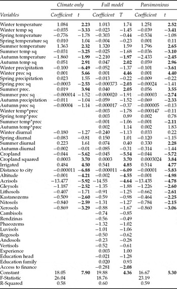
Table 1 presents three loglinear regressions on farmland value using the whole sample. In the first column, the “climate only” regression, the summer and winter climate coefficients are significant as well as autumn temperatures. In contrast, the seasonal diurnal coefficients are not significant.
Loglinear specifications of Ricardian model for Mexico

Number of observations is 621.
The full regression explores the complete set of soil variables and farmer characteristics. Several soils are not significant and most of the farmer characteristics remain insignificant. The greater the distance to the nearest city, the lower the farmland value. Access to loans is significant and negative. Of course, one would expect that having access to capital would be desirable. However, this variable actually measures the presence of loans amongst farmers and may be correlated with low net revenues and therefore endogenous.
The third regression includes climate interaction effects but drops the insignificant control variables. The temperature–precipitation interaction effects are not significant except for summer. In the summer, hotter and wetter farms have lower values.
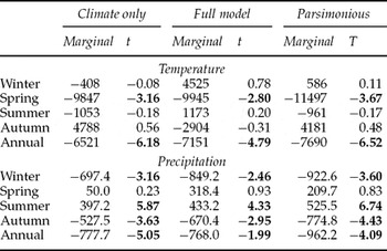
Table 2 calculates the marginal impact of climate for each regression in table 1. The marginals are stable across specifications. The annual temperature impacts range from −6,500 (−24%) to −7,700 (−28%) pesos per degree Celsius evaluated at the mean of the sample. The annual precipitation impacts range from −770 (−3%) to −960 (−4%) pesos per mm/mo. The harmful temperature effects are due to spring temperatures and the harmful precipitation effects are due largely to winter effects. The model also suggests that summer precipitation is strictly beneficial.
Marginal impacts of climate on Mexican farmland values (Loglinear model)

Marginals calculated at mean climate for each sample based on coefficients in table 1.
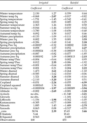
Table 3 compares irrigated versus rainfed farms. Both regressions have the same set of independent variables as the parsimonious regression. However, two soil types, acrisols and gleysols, are not observed in irrigated farms and so are not included in that regression. A formal F test of whether the climate coefficients from the rainfed and irrigated models are alike rejects that possibility.
Loglinear Ricardian models of rainfed and irrigated samples in Mexico

Note: The F-Statistic that irrigated and rainfed farm coefficients are the same is 3.04 and the critical value for an F (33,555) at 1% significance is 1.70.
The irrigated model in table 3 has few significant climate variables. Diurnal range is significant in every season except spring in the irrigated regression. Cropland, distance to city, altitude, and lithosols are all significant in the irrigated regression. There are some differences in the rainfed model. Most of the precipitation variables are significant in the rainfed regression. The autumn precipitation–temperature interaction term is significant in the rainfed regression whereas the spring precipitation–temperature interaction term is significant in the irrigated regression. More of the control variables in the rainfed regression are significant including cropland, cropland squared, distance to city, altitude, acrisols, and nitosols. This latter effect may be due to the larger sample size of the rainfed regression.
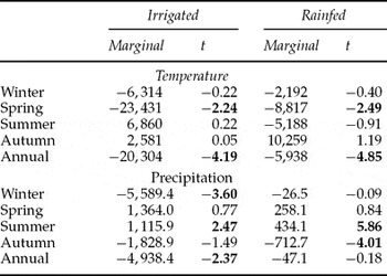
Table 4 examines the marginal impacts of climate in the rainfed and irrigated regressions of table 3. The temperature marginals for irrigated farms are much larger than the temperature marginals for rainfed farms. The temperature marginals are −20,300 pesos (−49%) per degree Celsius for irrigated farms, but they are only −5,900 pesos (−27%) per degree Celsius for rainfed farms. In both models, the harmful annual effect is being caused by large losses associated with warmer spring temperatures. Irrigated farms are also more sensitive to increases in precipitation compared to rainfed farms. The annual damages from increased precipitation are −4,940 pesos (−12%) per mm/mo for irrigated farms but only −50 pesos (−0.2%) per mm/mo for the rainfed farms. The harmful annual damages for irrigated farms are associated with winter precipitation.
Marginal climate impacts for Mexican rainfed and irrigated farms

Note: Marginals calculated at mean climate for each sample based on coefficients in table 3.
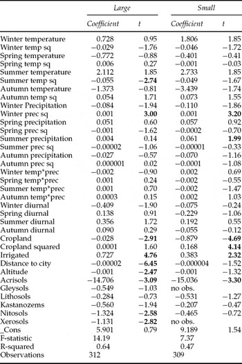
Table 5 tests whether small and large farms have the same climate sensitivity. Although few of the climate coefficients are individually significant, an F test reveals that climate coefficients of small and large farms are significantly different from each other. In addition, many of the control variables are significant in these regressions including cropland, irrigation, soils, altitude, cropland, and distance to city.
Comparison of small and large Mexican farms (Loglinear model)

Note: The F-statistic that large and small farm coefficients are the same is 2.35 where the critical value F (34, 553) at a 1% of significance level is 1.68.
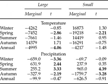
Table 6 examines the marginal climate impacts for small and large farms using the coefficients from table 5. The results indicate that the marginal temperature effects for large farms are larger than the marginal effects for small farms. Higher annual temperatures reduce large farm land values by −5,000 pesos (−32%) per degree Celsius and they reduce small farm land values by −4,200 pesos (−11%) per degree Celsius. This is due in large part to the harmful effects of warmer springs. Precipitation impacts are larger for small farms than large farms. More rain reduces large farm land values by −100 pesos (−0.6%) per mm/mo and reduces small farm land value by −630 pesos (−1.6%) per mm/mo. Because the seasonal effects are offsetting the annual marginal impacts are not significant. The differences in climate sensitivity between small and large farms may reflect specialization on one hand and the ability to find substitutes on the other.
Marginal climate impacts for Loglinear regressions on large and small Mexican farms

Marginals calculated at mean climate for each sample based on coefficients in table 5.
5. Projections with climate scenarios
We use the estimated regressions in the previous section to explore how future climate change scenarios might affect cropland in Mexico. The Ricardian results prove that farmland values vary across existing climates in Mexico. The marginals imply that a small change in temperature would have immediately harmful effects on Mexican agriculture. We now wish to explore the magnitude of impacts if climate changes a great deal. We use the estimated Ricardian functional forms to predict how future climates might affect future farmland values. These projections assume that all other conditions are held constant. We consequently are not making a forecast of how farmland values will actually change. We are simply isolating the effect of climate change on farmland values. We are not taking into account other likely changes such as in prices, investment, population, and technology.
We examine a set of climate change scenarios for 2100 predicted by three climate models: Center for Climate System Research (MIMR) (Hasumi and Emory, Reference Hasumi and Emori2004), Hadley Centre for Climate Prediction and Research (HADCM3) (Pope et al., Reference Pope, Gallani, Rowntree and Stratton2000), and the Parallel Climate Model (PCM) (Washington et al., Reference Washington, Weatherly, Meehl, Semtner, Bettge, Craig, Strand, Arblaster, Wayland, James and Zhang2000). For each climate scenario, we add the predicted change in temperature from the climate model (2070–2100 minus 1970–2000) to the baseline temperature in each district. We also multiply the predicted percentage change in precipitation from the climate models (2070–2100 minus 1970–2000 divided by 1970–2000) times the baseline precipitation in each district or province. This gives us a new climate for every district in Mexico. The PCM scenario is relatively mild, predicting a 2.3°C warming in Mexico and a reduction of 1.7 mm/mo in annual precipitation. The MIMR scenario predicts an average increase of 5.1°C and a precipitation reduction of 3.6 mm/mo. The HADCM3 scenario predicts a temperature increase of 5.1°C with a small increase of 0.4 mm/mo of precipitation. The models also differ slightly in the distribution of climate changes predicted across Mexico.
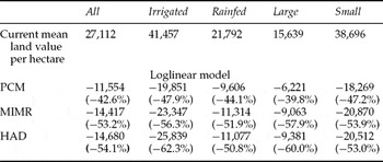
Table 7 presents the predictions from each climate scenario. The parsimonious regression in table 1 is used to predict impacts for the whole sample. The regressions in table 3 are used to predict impacts for rainfed and irrigated farms. The regressions in table 5 are used to predict impacts for small and large farms. In each case, we calculate the change in farmland value per hectare for each climate scenario in each municipio in Mexico. We then average the change in farmland values across all of Mexico to get a total impact for the country. Losses were limited to the value of the farm. That is, the most a farm can lose is 100% of its value.
Welfare impacts on Mexican farmland of alternative climate scenarios for 2100

Impacts are changes in land value in pesos per ha averaged over total farms. Percentage changes are in parentheses. Harmful impacts have been truncated to be no larger than the value of the land itself. All effects are statistically significant.
The models predict average losses with all three climate scenarios of between −42% and −50% of land value. The smaller losses were associated with the milder PCM scenario. Irrigated farms had larger absolute losses than small farms but the percentage losses were similar for all farms in each scenario except the HADCM3 scenario. The absolute losses were larger for small compared to large farms but the percentage losses were mixed. For the PCM scenario, small farms had larger percentage losses, for MIMR, they were about the same, and for HADCM3, large farms had larger percentage losses. Although the sample of all Mexican farms lost about half of its value, some farms lost all of their value. Between 30% and 45% of the farms in the sample lost 100% of their value depending on the climate scenario.
The effects vary a great deal across Mexico. Color figures of the results are provided in Appendix 2 (available at http://journals.cambridge.org/EDE). The maps display the results for each municipio in Mexico, the lowest level of political administration in Mexico (similar to the county in the United States). The map of the PCM result shows that although there are not wide differences in impacts, the impacts are not uniform across Mexico. The Baja Peninsula in the West, the northern mountains, and the southern Gulf coast suffer lower damages. These regions are either already cool or they are predicted to have smaller climate changes. There are even scattered municipios in the southern Gulf Coast near the state of Tabasco that are predicted to have higher farmland values. The map of the MIMR scenario shows that the impacts are generally more severe than the predicted PCM impacts and the range of effects is wider. The hardest hit regions are along the mid and southern Pacific coast and in the state of Veracruz along the southern Gulf coast. Many of these farms lose their entire value. Although they suffer small damages, the same regions that do well in the PCM scenario also do relatively better in the MIMR scenario. The map of the HADCM3 climate scenario results is similar to the MIMR scenario. HADCM3 also predicts severe damages along the mid and southern Pacific coast but beneficial impacts near the state of Tabasco. However, the HADCM3 model also predicts large losses along the northern border with Texas. Although the three climate scenarios have some similarities, there are clearly some marked differences amongst them.
6. Conclusion and policy implications
The analysis reveals that farmland values in Mexico are sensitive to climate. A marginal increase in annual temperature reduces land value by −6,500 to −7,700 pesos per degree Celsius. Even with adaptation, a small amount of warming is likely to have a negative impact on Mexican agriculture. A marginal increase in precipitation in every season is predicted to reduce farmland value. However, this annual effect is due largely to the harmful consequences of autumn and winter rainfall. Summer rainfall is beneficial. It is not clear why winter rainfall is so harmful in Mexico. The autumn rainfall can be tied to hurricanes. These results are consistent with earlier findings from South America (Seo and Mendelsohn, Reference Seo and Mendelsohn2008a).
Separating small and large farms and conducting Ricardian analysis on each sample reveals that both farm sizes are sensitive to warming. Annual temperature has a similar harmful impact on both small and large farms. The seasonal precipitation effects are significant but offsetting so that the annual precipitation effect is not significant. Wetter summers are beneficial and wetter autumns are harmful. Both seasonal effects are larger for small farms than large farms.
Both irrigated and rainfed farms are damaged by warmer temperatures. However, irrigated farms are more sensitive to warming than rainfed farms in Mexico. This result is consistent with findings from South America (Seo and Mendelsohn, Reference Seo and Mendelsohn2008a). The annual marginal precipitation effects are significant and negative only for irrigated farms. This result is not consistent with the results from South America that found the rainfed farms were far more sensitive than irrigated farms (Seo and Mendelsohn, Reference Seo and Mendelsohn2008a). The marginal precipitation effects, however, are dominated by harmful effects during winter, not during the growing season.
Future climate scenarios paint a bleak picture for Mexican agriculture. The loglinear model predicts average losses between 42% and 54%. Between 30% and 45% of the farms in the sample lose 100% of their value depending on the climate scenario. Irrigated farms are predicted to be slightly more vulnerable than rainfed farms to future climate scenarios. The results comparing the impacts of small and large farms are mixed depending on the climate scenario. These results are consistent with earlier findings from South America (Seo and Mendelsohn, Reference Seo and Mendelsohn2008a).
Projections of future impacts suggest that the impacts will vary a great deal across the Mexican landscape. Regions along the mid and southern Pacific coast look especially vulnerable to warming. Part of the northern mountain regions and the state of Tabasco may be the only regions that benefit. The rest of Mexico will be harmed but to a lesser extent. It is important that policy makers realize that the impacts will vary across the landscape and target farms appropriately.
If Mexican farmers are hurt by future climate scenarios, this will pose additional concerns for Mexico as many farm families are poor and with little education. There is reason to be concerned that people will migrate from especially unproductive regions to the cities as temperatures warm (Rivera and Yúnez-Naude, Reference Rivera and Yúnez-Naude2008).
This study has taken into account adaptations that farmers can make to climate change. The study has not evaluated adaptations that governments might take. Producing more effective varieties and breeds that might be more suited for a warmer world may provide farmers with useful substitutes for current crops and livestock. Providing farmers with more secure property rights to their water and lands may help provide incentive for farmers to invest more heavily in irrigated farming. Managing water more efficiently may help as part of a larger strategy to make irrigation more effective in Mexico.
International agencies may want to provide direct assistance to affected farmers. Providing micro credit may help especially poorer farm households make needed investments into capital to improve their farms. Providing access to new crop varieties and animals may help farmers adapt to future warmer climates. However, agencies must be careful not to subsidize farmers to remain in harm's way. It is critical that farmers adjust to the new conditions that are evolving because of warming. Providing insurance or emergency relief to compensate farmers for climate losses may hinder the adaptation that is needed and keep people in a steady state of need.
Appendix 1: Summary statistics of Mexican sample

1574 observations, 153 irrigated and 421 rainfed.
2477 observations, 126 irrigated and 351 rainfed.
3477 observations, 123 irrigated and 354 rainfed.
Source: ENHRUM, 2003.