1. Introduction
Since the 1970s, with the era of space missions, an increased interest has grown in investigating the solar wind–magnetosphere–ionosphere (SMI) coupling and dynamics with the aim of understanding and forecasting geomagnetic disturbances (Joselyn Reference Joselyn1985; Detman & Vassiliadis Reference Detman and Vassiliadis1997; Gonzalez, Tsurutani & Clúa de Gonzalez Reference Gonzalez, Tsurutani and Clúa de Gonzalez1999; Lindsay, Russell & Luhmann Reference Lindsay, Russell and Luhmann1999; Akasofu Reference Akasofu2001; Wing et al. Reference Wing, Johnson, Jen, Meng, Sibeck, Bechtold, Freeman, Costello, Balikhin and Takahashi2005; Lakhina & Tsurutani Reference Lakhina and Tsurutani2016; Camporeale et al. Reference Camporeale, Wing, Johnson, Jackman and McGranaghan2018; Baker Reference Baker2020; Borovsky Reference Borovsky2020). The history of characterizing and forecasting the geospace response to solar wind changes had begun in the 1930s with the pioneering work by Chapman & Ferraro (Reference Chapman and Ferraro1930), firstly introducing the concept of a magnetic cavity around the Earth, i.e. the magnetosphere. Starting from that, a new branch of space physics was born to infer the course of events during magnetic storms and substorms (Siscoe Reference Siscoe2001; McPherron Reference McPherron2020).
Nowadays, it is widely accepted that the Earth's magnetosphere is a multiscale complex system whose dynamics can be described as a far-from-equilibrium nonlinear system (Consolini, De Michelis & Tozzi Reference Consolini, De Michelis and Tozzi2008; Borovsky & Valdivia Reference Borovsky and Valdivia2018). This behaviour, associated with both an intrinsic nonlinear character and an externally driven topology due to the solar wind variability (Tsurutani et al. Reference Tsurutani, Sugiura, Iyemori, Goldstein, Gonzalez, Akasofu and Smith1990, Reference Tsurutani, Gonzalez, Tang and Lee1992), displays different features such as scale invariance and criticality (Consolini & De Michelis Reference Consolini and De Michelis1998; Consolini & Chang Reference Consolini and Chang2001, Reference Consolini and Chang2002; Uritsky et al. Reference Uritsky, Klimas, Vassiliadis, Chua and Parks2002; Consolini & De Michelis Reference Consolini and De Michelis2005), intermittency and turbulence (Consolini, Marcucci & Candidi Reference Consolini, Marcucci and Candidi1996; Consolini & De Michelis Reference Consolini and De Michelis1998) and low-dimensional chaos (Vassiliadis et al. Reference Vassiliadis, Sharma, Eastman and Papadopoulos1990; Klimas et al. Reference Klimas, Vassiliadis, Baker and Roberts1996). These features are associated with processes and phenomena operating at different spatial and temporal scales such as high-latitude energy deposition mechanisms (Ahn, Akasofu & Kamide Reference Ahn, Akasofu and Kamide1983), magnetotail disruption (Lui Reference Lui2016), central plasma sheet dynamics (Vörös et al. Reference Vörös, Baumjohann, Nakamura, Runov, Volwerk, Takada, Lucek and Rème2007), particle precipitation mechanisms and couplings between magnetospheric and ionospheric current systems (Daglis et al. Reference Daglis, Livi, Sarris and Wilken1994, Reference Daglis, Thorne, Baumjohann and Orsini1999). Such mechanisms and phenomena give rise to different critical issues in correctly forecasting the magnetospheric response to solar wind changes, especially at time scales of the order of a few minutes, where these processes typically operate (Consolini, Alberti & De Michelis Reference Consolini, Alberti and De Michelis2018).
One of the main reasons for the difficulties in providing a reliable forecast can be explained by considering that the magnetospheric dynamics comprises both the internal dynamics and the solar wind directly driven/triggered processes which act on different time scales. As recently shown (Alberti et al. Reference Alberti, Consolini, Lepreti, Laurenza, Vecchio and Carbone2017), a poorly significant correlation has been found at time scales lower than 200 minutes during geomagnetic storms, supporting the idea that a better forecasting of the magnetospheric response requires the knowledge of proxies capable of quantifying the internal magnetotail state, that is independent of the solar wind variations (Alberti et al. Reference Alberti, Lekscha, Consolini, De Michelis and Donner2020). Conversely, the significant correlation observed at long time scales (i.e. longer than 200 minutes) between solar wind variations and geomagnetic variability supports the possibility of providing a good estimate of geomagnetic index changes at hourly resolution (Pallocchia et al. Reference Pallocchia, Amata, Consolini, Marcucci and Bertello2006) (see also considerations in Siciliano et al. Reference Siciliano, Consolini, Tozzi, Gentili, Giannattasio and De Michelis2021). All the above difficulties have been shown to characterize machine-learning and artificial neural networks approaches, Burtons models and regression analysis, posing a serious concern for the correct estimation of short time-scale fluctuations that are extremely important in the framework of Space Weather studies, being the fast and large variations of the geomagnetic field, the most effective and dangerous for anthropic systems (Camporeale et al. Reference Camporeale, Wing, Johnson, Jackman and McGranaghan2018; Tozzi et al. Reference Tozzi, De Michelis, Coco and Giannattasio2019).
The main aim of this paper is to go deeper into the storm–substorm relationship by searching for phase coherence and relations between the AL and SYM-H geomagnetic indices. This constitutes a follow-up of previous works where amplitude relations have been investigated (e.g. Alberti et al. Reference Alberti, Consolini, Lepreti, Laurenza, Vecchio and Carbone2017, Reference Alberti, Lekscha, Consolini, De Michelis and Donner2020). Instead of using a large set of geomagnetic indices, as in Alberti et al. (Reference Alberti, Consolini, Lepreti, Laurenza, Vecchio and Carbone2017), we only focus on AL and SYM-H being representative proxies of magnetic substorms and storms, respectively (De Michelis et al. Reference De Michelis, Consolini, Materassi and Tozzi2011). These two indices, both at 1 min resolution, are indeed capable of resolving the small-scale variations due to storm triggering mechanisms (Wanliss & Showalter Reference Wanliss and Showalter2006; Wanliss & Uritsky Reference Wanliss and Uritsky2010) and impulsive energy release mechanisms due to the magnetotail activity during substorms (Klimas et al. Reference Klimas, Vassiliadis, Baker and Roberts1996).
Historically, the storm–substorm relations are investigated by means of searching for amplitude relations, while less attention has been paid to phase relations. To this latter purpose the wavelet transform (WT), successfully applied to several fields, ranging from climate (Yiou, Sornette & Ghil Reference Yiou, Sornette and Ghil2000; Taricco et al. Reference Taricco, Mancuso, Ljungqvist, Alessio and Ghil2015; Barbosa & Donner Reference Barbosa and Donner2016; Ekhtiari et al. Reference Ekhtiari, Agarwal, Marwan and Donner2019) to solar physics (Laurenza, Storini & Moreno Reference Laurenza, Storini and Moreno2005; Donner & Thiel Reference Donner and Thiel2007; Vecchio & Carbone Reference Vecchio and Carbone2009), with some applications also to the field of Space Weather (Consolini Reference Consolini1997; Consolini & Lui Reference Consolini and Lui2000; Materassi & Mitchell Reference Materassi and Mitchell2007; Laurenza et al. Reference Laurenza, Storini, Giangravè and Moreno2009; Kunagu et al. Reference Kunagu, Balasis, Lesur, Chandrasekhar and Papadimitriou2013; Zaourar et al. Reference Zaourar, Hamoudi, Mandea, Balasis and Holschneider2013; Balasis et al. Reference Balasis, Daglis, Mann, Papadimitriou, Zesta, Georgiou, Haagmans and Tsinganos2015), is employed to investigate energy–time–time-scale distribution as well as the phase coherence between the two geomagnetic indices. As highlighted in several previous works (e.g. De Michelis et al. Reference De Michelis, Consolini, Materassi and Tozzi2011; Runge et al. Reference Runge, Balasis, Daglis, Papadimitriou and Donner2018; Stumpo et al. Reference Stumpo, Consolini, Alberti and Quattrociocchi2020), when dealing with correlations between two quantities driven by a third one (such as in the SMI system), the mutual influence cannot be correctly evaluated if the common driver is not excluded. Thus, the partial wavelet coherence tool is here used to provide, for the first time, the evidence of phase relations between geomagnetic indices due to the internal dynamics of the magnetosphere by neglecting the common solar wind driver, as described by the $z$ component of the interplanetary magnetic field Bz.
2. Data
This work is based on the use of geomagnetic indices and solar wind parameters as freely retrieved from the OMNI database at https://cdaweb.gsfc.nasa.gov/index.html/. Specifically, the geomagnetic variability is monitored by using 2 geomagnetic indices: one high-latitude index, AL, and one low-latitude index, SYM-H. The former allows us to monitor the ionospheric auroral westward electrojet (Davis & Sugiura Reference Davis and Sugiura1966), associated with the impulsive activity of the magnetotail during magnetospheric substorms, while the latter is intended to quantify the activity of the ring current in the course of a geomagnetic storm (Iyemori Reference Iyemori1990). All geomagnetic indices have a 1 minute time resolution and are derived from longitudinally distributed chains of high (AL) and low (SYM-H) latitude ground-based magnetometers. As a solar wind proxy we use the $z$ component of the interplanetary magnetic field Bz in the geocentric solar magnetospheric (GSM) coordinate system.Footnote 1 We use Bz since it has been shown to be the best parameter for investigating the geomagnetic response to solar wind changes (Runge et al. Reference Runge, Balasis, Daglis, Papadimitriou and Donner2018; Stumpo et al. Reference Stumpo, Consolini, Alberti and Quattrociocchi2020).
For the present study, the superstorm that occurred on 20 November 2003 has been selected, being one of strongest storms of solar cycle 23 with $K_p= 9^-$ andFootnote 2 with the best data coverage for both solar wind parameters and geomagnetic indices, with no data gap for the selected parameters. For this reason, we used data covering the time interval between 16 November and 24 November, allowing us to take into account both the storm period and the quiet-time levels before and after the disturbance. With our time series at 1 minute resolution, our dataset consists of $N_p = 11\ 520$
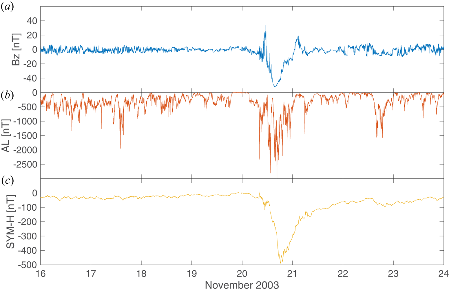
 points. Figure 1 reports the time series of the considered quantities (Bz, AL and SYM-H) for the selected period relative to the geomagnetic storm that occurred on 20 November 2003.
Temporal behaviour of the solar wind parameter Bz (a), the high-latitude geomagnetic index AL (b) and low-latitude geomagnetic index SYM-H (c) during the selected period relative to the geomagnetic storm that occurred on 20 November 2003.

The superstorm was associated with a high-speed full-halo coronal mass ejection originating from the active region AR 10501 on 18 November, located at N03E09 (Srivastava et al. Reference Srivastava, Mathew, Louis and Wiegelmann2009; Grechnev et al. Reference Grechnev, Uralov, Chertok, Slemzin, Filippov, Egorov, Fainshtein, Afanasyev, Prestage and Temmer2014). Several M-class flares were released from this active region, with the most intense an M3 class 07:52 UT, together with strong radio bursts (both type II and type IV). We observe that the Bz component, starting from 07:30 UT on 20 November, dropped rapidly to strongly negative values (${\rm Bz}_{\min } = -50\ {\rm nT}$ ), with long-lasting negative values from approximately 11:00 UT to 23:00 UT on 20 November. From the geomagnetic side we observe an intense activity of the westward auroral electrojet, with ${\rm AL}_{\min } \sim -2500$
 nT, suggesting an intense burst of activity in the magnetotail due to the solar wind changes. Furthermore, associated with the positive to negative variations of the interplanetary magnetic field Bz and with a time delay of ${\sim }90$
 minutes due to the travel time for the solar wind perturbation to the Earth's surface, a sudden decrease to negative values is observed for the SYM-H index, reaching a minimum value SYM-H$_{\min } \sim -500$
 nT.
3. Wavelet analysis
3.1. Wavelet Transform
Since our measurements of both the solar wind and geomagnetic variability are obtained as time series whose dynamics usually manifests a nonlinear behaviour, a suitable method for detecting and quantifying nonlinearities in non-stationary time series is wavelet analysis (Torrence & Compo Reference Torrence and Compo1998). The main idea is to convolve a time series with a function satisfying certain conditions, i.e. the so-called wavelet (Daubechies Reference Daubechies1990; Farge et al. Reference Farge, Guezennec, Ho and Meneveau1990; Farge Reference Farge1992). Given a signal represented as a discrete time series $x_n$ with a fixed sampling time ${\rm \Delta} t$
 and a mathematical function $\psi (x) \in L^2(R)$
 with $x \in R$
 , if $\psi (x)$
 is a well-localized function with fast decay at infinity and at least one vanishing moment (i.e. zero mean), then $\psi (x)$
 can be termed a continuous ‘mother wavelet’ (Farge Reference Farge1992; Farge & Schneider Reference Farge and Schneider2015). Thus, the WT can be defined as

where $N_p$ is the length of the time series, $s$
 is the scale, ${\dagger}$
 denotes complex conjugation and $W_n(s)$
 is the wavelet coefficient (Torrence & Compo Reference Torrence and Compo1998). By varying $s$
 and translating along the time index $n$
 it is possible to reconstruct how the amplitude of the signal varies across scales and with time, thus providing an efficient way to investigate localized processes in the time-scale domain (Torrence & Compo Reference Torrence and Compo1998). In this way, we build up an additive decomposition of time series into components, usually describing the dynamics in logarithmically spaced frequency bands (Torrence & Compo Reference Torrence and Compo1998). Within the different possible choices for the function $\psi (x)$
 , usually called the mother wavelet, here, we use two different continuous complex functions that are suitable for evaluating the degree of coherence between pairs of quantities, i.e. the Morlet and the Paul wavelets.
The Morlet wavelet is defined as

with $\omega _0$ the dimensionless frequency and $x$
 the dimensionless time (Grossmann, Kronland-Martinet & Morlet Reference Grossmann, Kronland-Martinet and Morlet1989).
The Paul wavelet is instead defined as

with $m = 4$ the order of the wavelet and $i$
 the imaginary unit.
Both mother wavelets are well suited for investigating both amplitude and phase contributions in time series, although with different features. While the Morlet wavelet has a good frequency resolution with respect to its time localization, the narrower width resolution in the time domain makes the Paul function very localized in time (Farge et al. Reference Farge, Guezennec, Ho and Meneveau1990; Farge Reference Farge1992; Farge & Schneider Reference Farge and Schneider2015). The choice of $\omega _0 = 6$ for the Morlet wavelet and $m = 4$
 for the Paul wavelet is particularly suited for the analysis of signals whose components have a time-varying frequency and/or a time-varying amplitude (Holschneider Reference Holschneider1995; Maraun, Kurths & Holschneider Reference Maraun, Kurths and Holschneider2007). Another important and useful feature of both mother wavelets is the relationship between the scale parameter $s$
 and the Fourier period (i.e. the real time scale of oscillation) $\tau$
 , allowing us to detect the intrinsic periodicities of the analysed time series (Grinsted, Moore & Jevrejeva Reference Grinsted, Moore and Jevrejeva2004). For the Morlet this relation is $\tau = 1.06\ {\rm s}$
 , while for the Paul it is $\tau = ({4{\rm \pi} }/({2m+1}))s = 1.4\ {\rm s}$
 .
3.2. Wavelet spectrum and cross-spectrum
From the WT defined in (3.1), the wavelet power spectrum is $\mathcal {W}(\tau, t_n) = |W_n(\tau )|^2$ , where the relations $\tau = 1.06\ {\rm s}$
 and $\tau = 1.4\ {\rm s}$
 permit us to directly work in the time-scale domain. Furthermore, since the WT suffers from edge artefacts, because it is not completely localized in time, it is important to define a cone of influence (COI), where edge effects cannot be ignored. It is defined as the area where the wavelet power $\mathcal {W}(\tau, t_n)$
 decreases by a factor ${\rm e}^{-2}$
 due to a discontinuity at the edges (Torrence & Compo Reference Torrence and Compo1998; Grinsted et al. Reference Grinsted, Moore and Jevrejeva2004). Moreover, the statistical significance of $\mathcal {W}(\tau, t_n)$
 must be assessed with respect to the null hypothesis that the signal is associated with a stationary process with a background spectrum $\mathcal {P}(\tau )$
 . Since many natural time series show features of red noise that can be modelled via a first-order auto-regressive process, we assessed the statistical significance of $\mathcal {W}(\tau, t_n)$
 with respect to a background spectrum of the form

with $\alpha$ the lag-1 auto-correlation estimated from the observed time series (Allen & Smith Reference Allen and Smith1996).
The univariate wavelet analysis can be further extended to investigate the common power shared between two different signals by defining the so-called cross-WT (XWT) (Grinsted et al. Reference Grinsted, Moore and Jevrejeva2004; Maraun et al. Reference Maraun, Kurths and Holschneider2007). This method is based on the computation of the WT for two different signals $X(t)$ and $Y(t)$
 , namely $W_n(s)^X$
 and $W_n(s)^Y$
 , respectively. Then, XWT is simply defined as

As for the univariate WT, it is possible to define the cross-wavelet power as

The XWT is a helpful tool for investigating the existence of common power and relative phase in the time–time-scale space between two time series, although it cannot be used to disentangle any possible relations between them (Maraun & Kurths Reference Maraun and Kurths2004; Maraun et al. Reference Maraun, Kurths and Holschneider2007).
3.3. WT coherence
One of the most useful concepts within wavelet analysis is surely the so-called WT coherence (WTC). It is able to quantify how oscillatory components are coherent, i.e. to detect transient but significant localized correlations in the time–time-scale space (Grinsted et al. Reference Grinsted, Moore and Jevrejeva2004). Indeed, although two time series can share a significant amount of power, i.e. they can have a common power $\mathcal {W}(\tau, t_n)$ in a specific time–time-scale band; this cannot be associated with a significant interrelation between them (Maraun & Kurths Reference Maraun and Kurths2004). As introduced by Torrence & Webster (Reference Torrence and Webster1999) the WTC is defined as

with $\mathcal {S}$ a smoothing operator based on a weighted running average in both time and scale (Torrence & Webster Reference Torrence and Webster1999). As for usual correlation analyses, it is fundamental to assess the significance of correlation levels via Monte Carlo methods. For this purpose, a large ensemble of surrogate data is generated with similar lag-1 auto-correlation coefficients as the input time series. Then, for each pair of surrogate time series the wavelet coherence is evaluated. Finally, the significance level for each scale is estimated using only values outside the COI (Torrence & Webster Reference Torrence and Webster1999; Grinsted et al. Reference Grinsted, Moore and Jevrejeva2004; Maraun et al. Reference Maraun, Kurths and Holschneider2007).
3.4. Partial Wavelet Coherence
When investigating a complex system like the SMI one, it could happen that some components are interacting each other and this effect could bias correlation estimates. For example, having a system with two different components, namely $S_1$ and $S_2$
 , and assuming that both are related to an external forcing $F$
 , then the relation between $S_1$
 and $S_2$
 needs to be studied by removing the effect of the common driver $F$
 . For this reason Mihanović, Orlić & Pasarić (Reference Mihanović, Orlić and Pasarić2009) firstly introduced the concept of partial wavelet coherence (PWC) that allows us to evaluate the wavelet coherence between two time series $Y$
 and $X_1$
 after removing the influence of the time series $X_2$
 as

As a practical example: if $\text {WTC}(Y,X_1)$ is high but $\text {PWC}(Y,X_1,X_2)$
 is low, then $X_1$
 has no significant influence on $Y$
 , and $X_2$
 dominates the effect on $Y$
 ; if $\text {PWC}(Y,X_1,X_2) \sim \text {PWC}(Y,X_2,X_1)$
 then both $X_1$
 and $X_2$
 have a significant influence on $Y$
 (Mihanović et al. Reference Mihanović, Orlić and Pasarić2009; Ng & Chan Reference Ng and Chan2012). As for WTC, Monte Carlo methods are used for assessing the significance with respect to a red noise background spectrum (Allen & Smith Reference Allen and Smith1996; Grinsted et al. Reference Grinsted, Moore and Jevrejeva2004; Maraun et al. Reference Maraun, Kurths and Holschneider2007; Hu & Si Reference Hu and Si2016, Reference Hu and Si2021).
For our analysis we set the following parameters: minimum scale $\tau _{\min } = 2 {\rm \Delta} t = 2$ minutes, maximum scale $\tau _{\max } = 4096$
 minutes (the closest power of two to half of the length of the time series), ${\rm \Delta} j = 0.25$
 , i.e. we used 4 sub-octaves per octave, and a total number of scales $j_1 = ({\log _2(N_p)-1})/{{\rm \Delta} j} = 51$
 .
4. Results
4.1. Spectral features
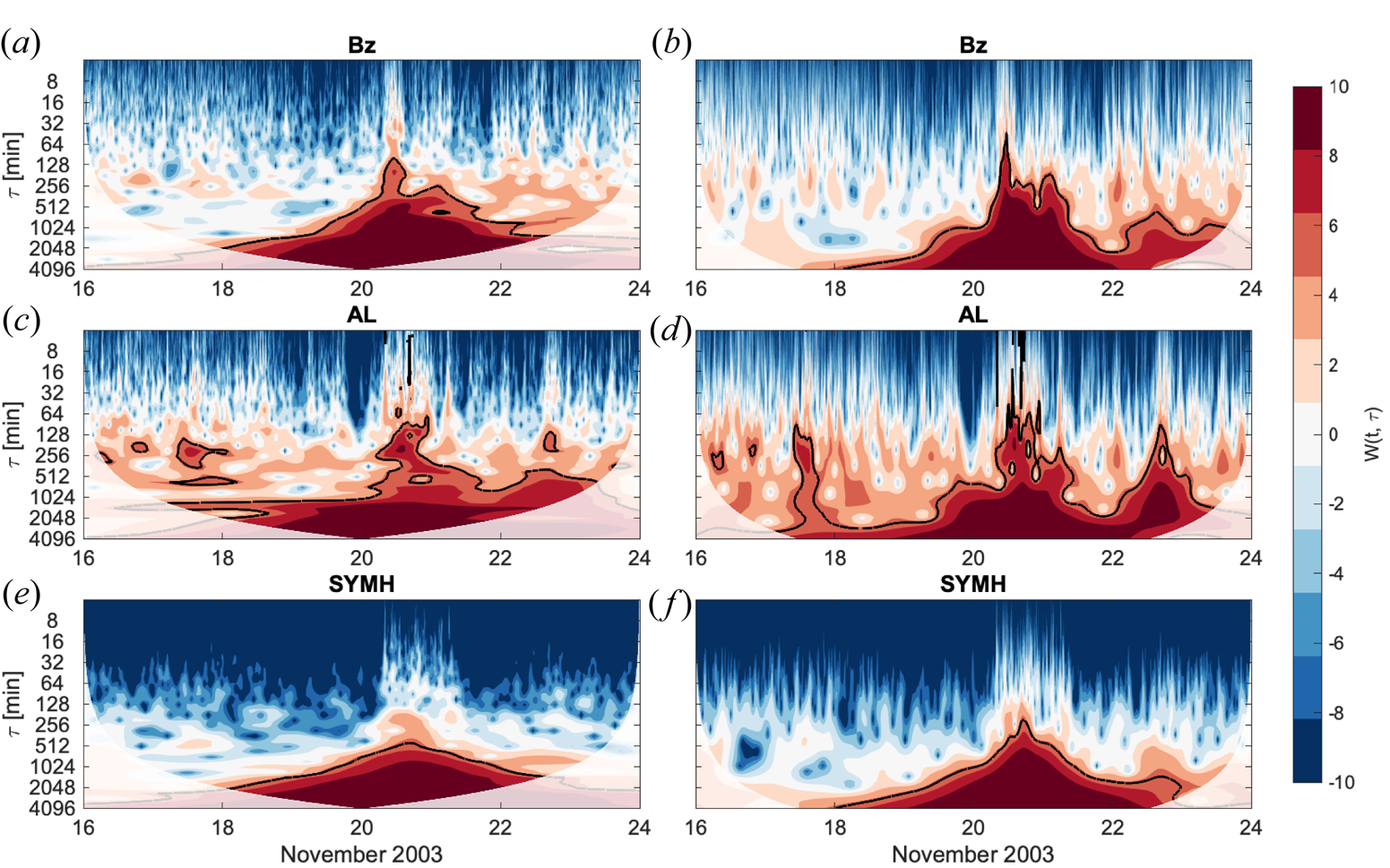
We start our investigation with the evaluation of the wavelet power in the time–time-scale plane, i.e. the so-called scalogram $\mathcal {W}(\tau, t_n)$ , for the three quantities used in our analysis, namely, Bz, AL and SYM-H, as reported in figure 2.
The scalogram $\mathcal {W}(\tau, t_n)$ (in logarithmic scale) for the three quantities: Bz (a,b), AL (c,d) and SYM-H (e,f ). The white area refers to the COI, while the 5 % significance level against red noise is shown as a thick contour. Panels (a,c,e) and (b,d,f) show the results using the Morlet and the Paul wavelets, respectively.

We observe that there are common features in the wavelet power between the three quantities, especially looking at the long-time-scale dynamics, namely $\tau \gtrsim 200$ min. It is interesting to note that the Paul wavelet (right panels in figure 2) appears to resolve better with the respect to the Morlet one (left panels in figure 2) the time localization of the observed features, such as for example the occurrence of the sharp transition due to the geomagnetic storm (see around 20 November) or the occurrence of substorm activity outside the disturbed period (see around 18 November or 23 November). Indeed, we have to recall that we can observe substorm activity also without the simultaneous observation of a geomagnetic storm (Lyons et al. Reference Lyons, Blanchard, Samson, Lepping, Yamamoto and Moretto1997; Lakhina & Tsurutani Reference Lakhina and Tsurutani2016; Lui Reference Lui2016). However, it is difficult to quantify the shared common patterns between time series by only looking at the univariate analysis. The WTC can be helpful in this regard.
4.2. Shared features
Before computing the WTC we note that the internal dynamics between ionospheric and magnetospheric current systems does not simultaneously occur (Daglis et al. Reference Daglis, Livi, Sarris and Wilken1994; De Michelis et al. Reference De Michelis, Consolini, Materassi and Tozzi2011). Furthermore, also the geomagnetic response does not simultaneously occur with solar wind changes but it is delayed by of the order of tens of minutes (Lyons et al. Reference Lyons, Blanchard, Samson, Lepping, Yamamoto and Moretto1997; Alberti et al. Reference Alberti, Consolini, Lepreti, Laurenza, Vecchio and Carbone2017). For this reason, we firstly need to evaluate the characteristic time delay between input and output quantities. For this purpose we use the delayed mutual information method (De Michelis et al. Reference De Michelis, Consolini, Materassi and Tozzi2011; Alberti et al. Reference Alberti, Consolini, Lepreti, Laurenza, Vecchio and Carbone2017; Johnson, Wing & Camporeale Reference Johnson, Wing and Camporeale2018). Given two time series $X$ and $Y$
 , the delayed mutual information coefficient $\text {MI}(\varDelta )$
 can be written as

where $p(x(t), y(t+\varDelta ) )$ is the joint probability of observing the pair of values ${(x(t), y(t+\varDelta)}$
 , while $p(x(t))$
 and $p(y(t))$
 are the probability distributions of observing $x(t)$
 and $y(t)$
 as independent quantities (Johnson et al. Reference Johnson, Wing and Camporeale2018). The choice of using the mutual information instead of a cross-correlation analysis allows us to recover not only linear coupling between pairs of quantities but also nonlinear ones (Johnson et al. Reference Johnson, Wing and Camporeale2018). Indeed, the mutual information is a measure of the uncertainty reduction in the knowledge of a specific quantity if knowing another. Thus, the high the mutual information the low is the reduction of uncertainty, while a zero mutual information means that two quantities are independent (De Michelis et al. Reference De Michelis, Consolini, Materassi and Tozzi2011; Johnson et al. Reference Johnson, Wing and Camporeale2018). The MI is particularly appropriated in the SMI framework because of the nonlinear features of the magnetosphere–ionosphere dynamics as well as its response to the solar wind variability (Alberti et al. Reference Alberti, Consolini, Lepreti, Laurenza, Vecchio and Carbone2017). To quantify the relevance of the degree of mutual information a significance threshold is required. This can be obtained by means of a certain number of surrogates (here 1000) of the two time series $X$
 and $Y$
 by randomly sorting them. In this way any time correlation in each sequence as well as any possible correspondence is disrupted without altering the statistics of the original time series. For each pair of surrogates, we evaluate the mutual information coefficient ${\rm MI}_0 = {\rm MI}(\varDelta = 0)$
 (the zero lag is justified since the two surrogates are independent). Then, the cumulative statistics of MI$_0$
 values is evaluated and the threshold level is chosen at the value MI$_t$
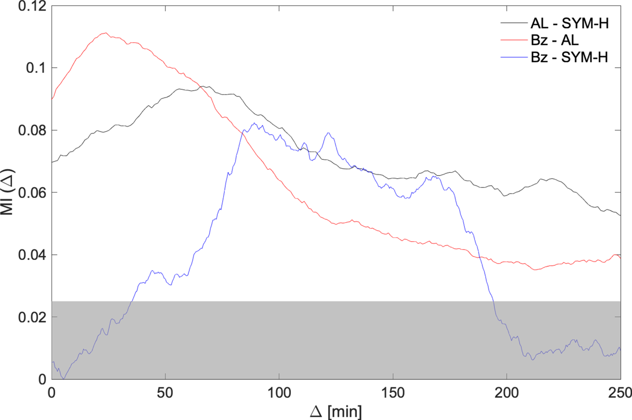
 at which the cumulative distribution function is 0.95. This corresponds to the 5 % confidence limit. Moreover, due to the finite data sample of the analysed time series the joint probability as well as the independent probabilities are evaluated via a non-parametric procedure known as kernel density estimation (Silverman Reference Silverman1986). This procedure is closely related to histograms although it allows us to reduce data sampling effects and to obtain a smoother distribution by using a suitable kernel. For this study, the Epanechnikov kernel is used, which is optimal in a mean square error sense (Epanechnikov Reference Epanechnikov1969). The characteristic time delay between the input and the output quantities is that associated with the maximum value of the mutual information coefficient (Alberti et al. Reference Alberti, Consolini, Lepreti, Laurenza, Vecchio and Carbone2017). As shown in figure 3, the obtained time delays are: $\varDelta = 67$
 minutes between AL and SYM-H, $\varDelta = 25$
 minutes between Bz and AL and $\varDelta = 86$
 minutes between Bz and SYM-H, respectively. These time delays are all consistent with previous works where the SMI coupling has been investigated (Lyons et al. Reference Lyons, Blanchard, Samson, Lepping, Yamamoto and Moretto1997; Alberti et al. Reference Alberti, Consolini, Lepreti, Laurenza, Vecchio and Carbone2017) as well as where the storm–substorm relations have been studied (Daglis et al. Reference Daglis, Livi, Sarris and Wilken1994; De Michelis et al. Reference De Michelis, Consolini, Materassi and Tozzi2011; Runge et al. Reference Runge, Balasis, Daglis, Papadimitriou and Donner2018; Stumpo et al. Reference Stumpo, Consolini, Alberti and Quattrociocchi2020).
The mutual information coefficient between AL and SYM-H (black line), Bz and AL (red line) and Bz and SYM-H (blue line), respectively. The horizontal dashed lines refer to the highest 95 % statistical significance level obtained for the three pairs of quantities.

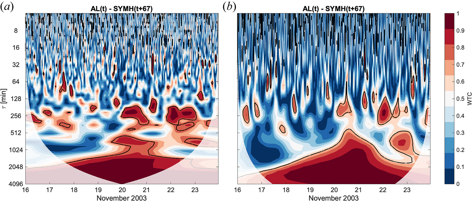
Having evaluated the corresponding time delays between pairs of variables, we can now characterize the phase dependence between AL and SYM-H by evaluating the WTC, $\text {WTC}(\tau, t_n)$ , as in (3.7). The results by using the Morlet and the Paul wavelets are reported in figure 4.
The WTC, $\text {WTC}(\tau, t_n)$ , (in logarithmic scale) between AL and SYM-H. The white area refers to the COI, while the 5 % significance level against red noise is shown as a thick contour. Panels (a,b) show the results using the Morlet and the Paul wavelets, respectively.

It is interesting to observe the widest area of significant coherence is mainly found on time scales longer than 5 hours, closely related to the observed break in the nonlinear response of the geomagnetic variability to the solar wind driver (Tsurutani et al. Reference Tsurutani, Sugiura, Iyemori, Goldstein, Gonzalez, Akasofu and Smith1990), with enhancements on shorter time scales only observed during the main phase and at the end of the geomagnetic storm. A significant coherence at large scales is also observed after the geomagnetic storm, close to the end of 22 November, that could be related to another small depression observed in the SYM-H index values towards negative values, in close correspondence to both enhancements in the AL index and a negative turning of Bz (see figure 2). These results seem to point towards the existence of an inter-relation between substorms and storms, as previously highlighted (e.g. Daglis et al. Reference Daglis, Livi, Sarris and Wilken1994; De Michelis et al. Reference De Michelis, Consolini, Materassi and Tozzi2011); however, we cannot draw any conclusion on the possible dependence of this coupling from a common driver due to the solar wind variability.
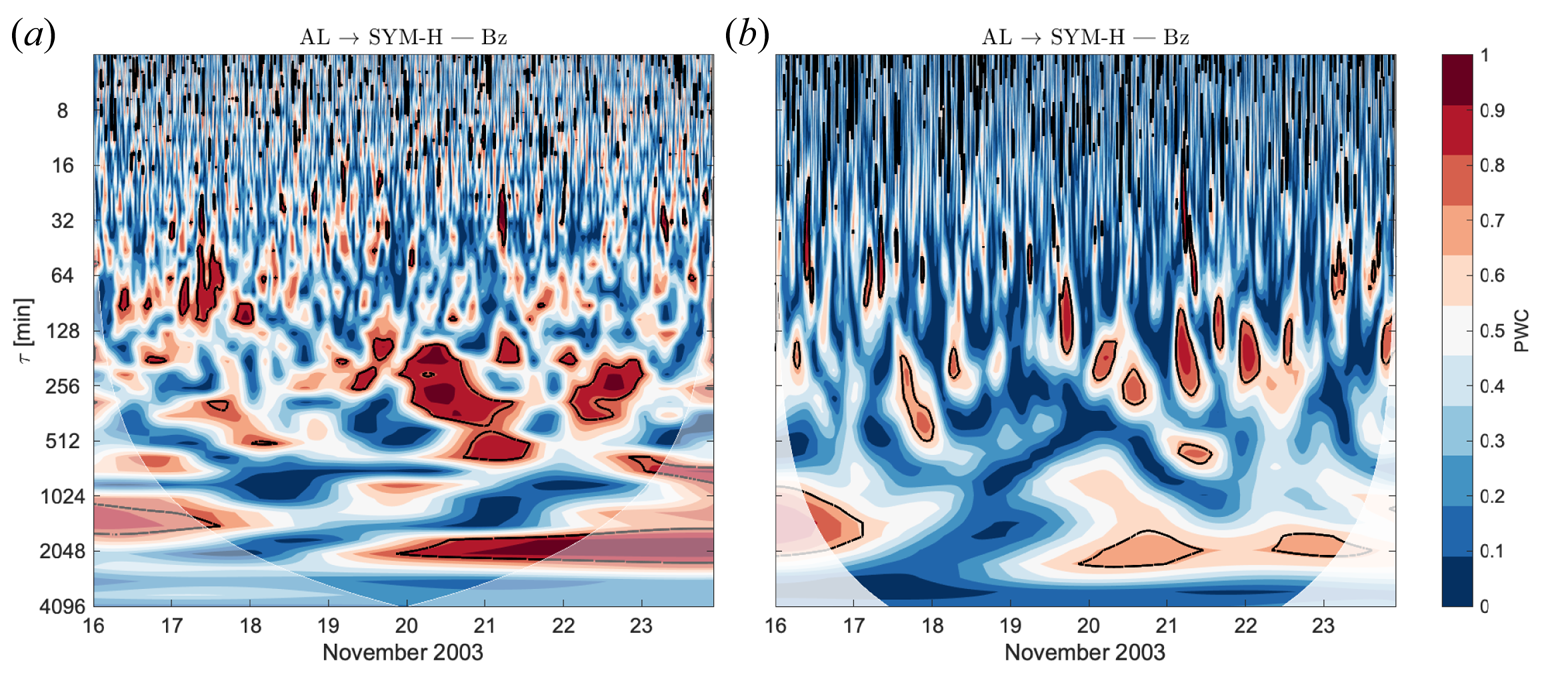
In order to speculate on the latter point we evaluate the PWC between AL and SYM-H by excluding Bz (see figure 5).
The PWC, $\text {PWC}(\tau, t_n)$ , (in logarithmic scale) between AL and SYM-H by excluding Bz. The white area refers to the COI, while the 5 % significance level against red noise is shown as a thick contour. Panels (a,b) show the results using the Morlet and the Paul wavelets, respectively.

When investigating the partial coherence between AL and SYM-H by neglecting the common driver Bz we can observe a reduction of the area of significant coherence at large time scales (i.e. $\tau \gtrsim 5$ h), while the previously observed coherence at shorter time scales around 200 minutes persists. This is especially evident during the main phase of the geomagnetic storm as well as in close correspondence to the secondary depression of the SYM-H index at the end of 22 November, after the recovery of the geomagnetic storm that occurred on 20 November (see figure 1). This can be clearly related to the enhancements observed at the same time in the AL index (see figure 1) that seem to produce a small depression in the SYM-H index values towards negative values (SYM-H $\sim -100$
 nT), partially related to a negative turning of Bz. Thus, this suggests that there is a clear coupling between Bz and AL which in turn can reflect on SYM-H. Moreover, instead of the wider area observed for the coherence at large time scales (see figure 4), the significant coherence at these time scales is only found for a narrower frequency band (around 2048 minutes). This area is close to the COI and could suffer of edge artefacts. The results are almost consistent by using both the Morlet and the Paul wavelets, apart, again, from the better temporal localization of the Paul with respect to the Morlet. This is valid at almost all time scales, also at around 2048 minutes, that could suggest that this time scale could be related to long-lasting phenomena related to the recovery phase of the geomagnetic storm. However, the main result remains practically unchanged, i.e. a clear substorm–storm relation emerges at time scales below/around the spectral break of the nonlinear response of the geomagnetic activity to the solar wind driver (Tsurutani et al. Reference Tsurutani, Sugiura, Iyemori, Goldstein, Gonzalez, Akasofu and Smith1990). This result is in agreement previous findings according to which there is a storm–substorm relation due to the ionospheric plasma (mainly oxygen ions) flowing towards the magnetospheric regions via field-aligned currents (Daglis et al. Reference Daglis, Livi, Sarris and Wilken1994). This produces fast enhancements of the ring current activity, particularly during the main phase of a geomagnetic storm (Daglis et al. Reference Daglis, Livi, Sarris and Wilken1994; De Michelis et al. Reference De Michelis, Consolini, Materassi and Tozzi2011). Moreover, these enhancements affect the typical times of processes operating during the recovery phase as charge exchange and wave–particle loss mechanisms, thus explaining our findings of coherence during this phase of the storm. These findings are in favour of the scenario according to which geomagnetic storms, although certainly driven by solar wind changes, can also be understood as a collection of substorms (Daglis et al. Reference Daglis, Thorne, Baumjohann and Orsini1999; Akasofu Reference Akasofu2001, Reference Akasofu2017), with the storm-time ring current mainly of terrestrial origin (Daglis Reference Daglis1997; De Michelis et al. Reference De Michelis, Consolini, Materassi and Tozzi2011; Stumpo et al. Reference Stumpo, Consolini, Alberti and Quattrociocchi2020).
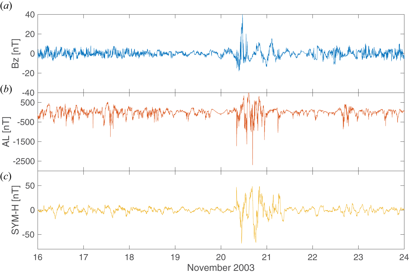
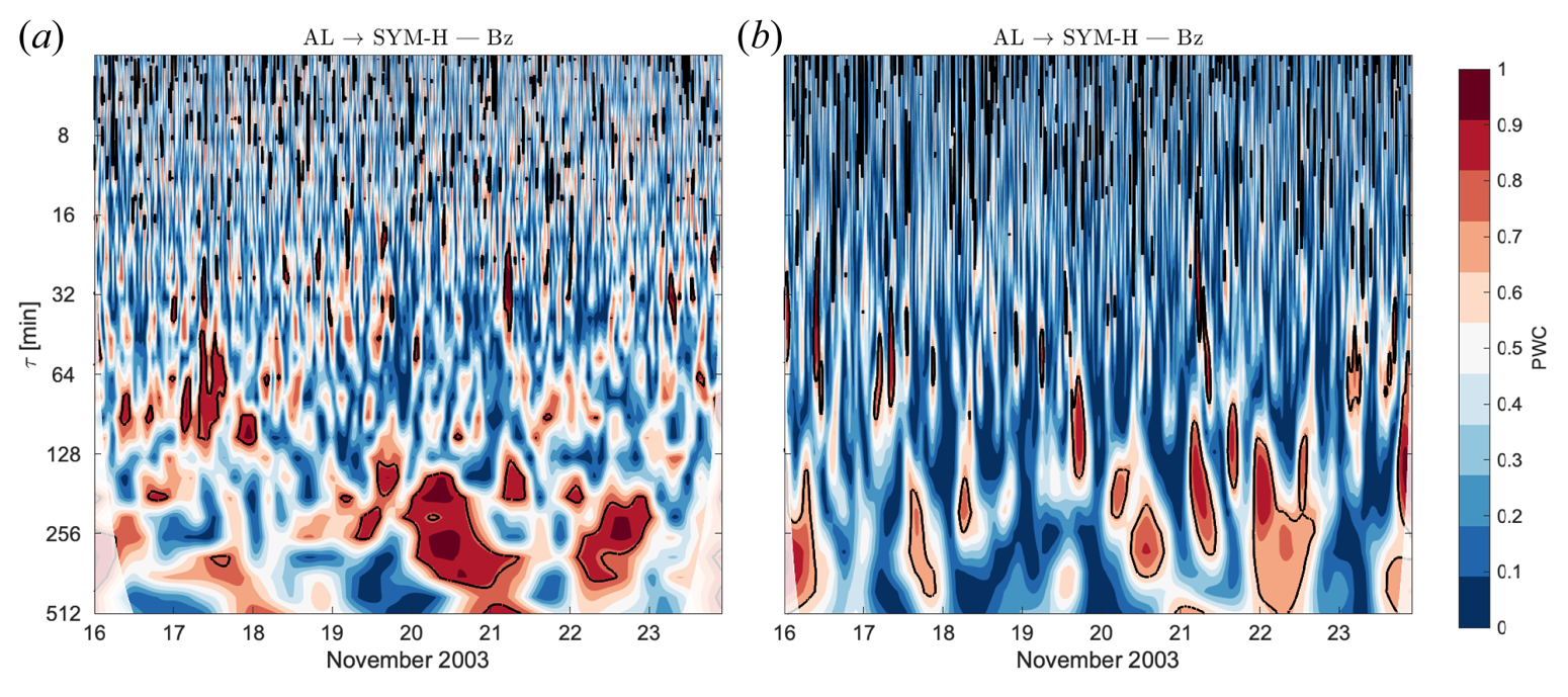
As a final step to assess our findings we performed the partial coherence analysis by removing the large-scale dynamics due to the coronal mass ejection hitting the Earth's magnetosphere. Indeed, as shown by Dolla et al. (Reference Dolla, Marqué, Seaton, Van Doorsselaere, Dominique, Berghmans, Cabanas, De Groof, Schmutz, Verdini, West, Zender and Zhukov2012), misleading information could be recovered for signals that are very similar on long time scales, although wavelet coherence can be performed without removing the large-scale trend (Maraun & Kurths Reference Maraun and Kurths2004; Maraun et al. Reference Maraun, Kurths and Holschneider2007; Dolla et al. Reference Dolla, Marqué, Seaton, Van Doorsselaere, Dominique, Berghmans, Cabanas, De Groof, Schmutz, Verdini, West, Zender and Zhukov2012). To this purpose, as in Dolla et al. (Reference Dolla, Marqué, Seaton, Van Doorsselaere, Dominique, Berghmans, Cabanas, De Groof, Schmutz, Verdini, West, Zender and Zhukov2012), we removed the large-scale trend by using a high-pass filter with a cutoff time scale of 512 minutes. This time scale corresponds to the closest power of two to the double time scale break of $\tau _b \sim 5$ hours observed by Tsurutani et al. (Reference Tsurutani, Sugiura, Iyemori, Goldstein, Gonzalez, Akasofu and Smith1990) in the nonlinear response to the solar wind changes. The choice of $2 \tau _b$
 as cutoff time scale is to take into account edge effects due to both the filtering procedure and the wavelet analysis. Figure 6 reports the filtered time series, while figure 7 reports the results of the PWC between AL and SYM-H by excluding Bz with the large-scale trend removed from each time series. The results shown in figure 7 match those in figure 5, thus confirming the physical meaning of our findings on observed coherence at shorter time scales of around or less than 5 hours. This is again evident during the main phase of the geomagnetic storm as well as in close correspondence with the secondary depression of the SYM-H index at the end of 22 November.
Temporal behaviour of the solar wind parameter Bz (a), the high-latitude geomagnetic index AL (b) and low-latitude geomagnetic index SYM-H (c) during the selected period relative to the geomagnetic storm occurred on 20 November 2003 when the large-scale trend is removed.

The PWC $\text {PWC}(\tau, t_n)$ (in logarithmic scale) between AL and SYM-H by excluding Bz with the large-scale trend removed from each time series. The white area refers to the COI, while the 5 % significance level against red noise is shown as a thick contour. Panels (a,b) show the results using the Morlet and the Paul wavelets, respectively.

5. Discussion and conclusions
In this study we investigated the storm–substorm relationship by using different measures developed in the context of wavelet analysis (Torrence & Compo Reference Torrence and Compo1998; Mihanović et al. Reference Mihanović, Orlić and Pasarić2009; Ng & Chan Reference Ng and Chan2012; Hu & Si Reference Hu and Si2016, Reference Hu and Si2021). Our results underline the existence of an inter-relation between substorms and storms that mainly emerges at time scales below/around the spectral break of the nonlinear response of the geomagnetic activity to the solar wind driver ($\sim 5$ h, Tsurutani et al. Reference Tsurutani, Sugiura, Iyemori, Goldstein, Gonzalez, Akasofu and Smith1990). Although the storm–substorm coupling has been previously investigated and highlighted in different works (Daglis et al. Reference Daglis, Livi, Sarris and Wilken1994; De Michelis et al. Reference De Michelis, Consolini, Materassi and Tozzi2011; Runge et al. Reference Runge, Balasis, Daglis, Papadimitriou and Donner2018; Stumpo et al. Reference Stumpo, Consolini, Alberti and Quattrociocchi2020), the main novelty of this study consists in the identification of the time scales of processes involved in this coupling. Moreover, by means of the partial coherence analysis we are able to investigate this coupling by neglecting the solar wind driver, as described by means of Bz. In this way, we clearly observe a reduction of the area of significant coherence at large time scales (i.e. $\tau \gtrsim 5$
 h), while a significant coherence persists at shorter time scales. These findings taken together seem to confirm that there is a non-negligible information coming from the internal variability of the magnetosphere–ionosphere system as a result of a complex interplay between processes and phenomena of internal origin, triggered by external processes. Thus, the following scenario can be drawn to explain our findings. During geomagnetic storms the magnetospheric ring current intensity increases due to the outflow of high-latitude oxygen ions O$^+$
 of ionospheric origin related to the field-aligned currents activation (Daglis et al. Reference Daglis, Livi, Sarris and Wilken1994), although the high-latitude auroral activity is related to loading–unloading processes taking place in the magnetotail region (Ahn et al. Reference Ahn, Akasofu and Kamide1983; Akasofu Reference Akasofu2001, Reference Akasofu2017). This means that the low-latitude geomagnetic activity is triggered via internal mechanisms of high-latitude ionospheric origin which in turn are driven by processes taking place at the boundary between the magnetosphere and the interplanetary medium, mainly related to reconnection processes and convective phenomena related to the solar wind variability (Ahn et al. Reference Ahn, Akasofu and Kamide1983; Tsurutani et al. Reference Tsurutani, Sugiura, Iyemori, Goldstein, Gonzalez, Akasofu and Smith1990; Lyons et al. Reference Lyons, Blanchard, Samson, Lepping, Yamamoto and Moretto1997; Akasofu Reference Akasofu2001; Lui Reference Lui2016). Our results clearly support these mechanisms (see figure 5). Indeed, the observed significant coherence between AL and SYM-H when neglecting the common driver Bz on time scales around 5 hours during the main phase of the geomagnetic storm explains the storm–substorm coupling due to ionospheric plasma flowing towards the magnetospheric regions (Daglis et al. Reference Daglis, Livi, Sarris and Wilken1994, Reference Daglis, Thorne, Baumjohann and Orsini1999). Thus, geomagnetic storms, although mainly driven by solar wind changes, can also be understood as a collection of substorms (Daglis et al. Reference Daglis, Thorne, Baumjohann and Orsini1999; Akasofu Reference Akasofu2001), with the storm-time ring current mainly of terrestrial origin (Daglis Reference Daglis1997; De Michelis et al. Reference De Michelis, Consolini, Materassi and Tozzi2011; Stumpo et al. Reference Stumpo, Consolini, Alberti and Quattrociocchi2020).
The main message of this work is that a significant amount of information comes from the interactions between geomagnetic storms and magnetospheric substorms. The latter represent one of the most challenging problems in space physics (Manshour et al. Reference Manshour, Balasis, Consolini, Papadimitriou and Paluš2021) and has a crucial impact on any forecasting tool, involving time scales of the order of a few minutes, where the forecasting horizon significantly reduces (Consolini et al. Reference Consolini, Alberti and De Michelis2018). Indeed, due to the different internal processes taking place during a geomagnetic storm such as loading–unloading mechanisms (Kamide & Kokubun Reference Kamide and Kokubun1996; Akasofu Reference Akasofu2001, Reference Akasofu2017), wave–particle coupling, fast relaxation processes (Vörös et al. Reference Vörös, Baumjohann, Nakamura, Runov, Volwerk, Takada, Lucek and Rème2007) and magnetotail phenomena (Lui Reference Lui2016), a precise forecasting of short time scales is difficult. However, since the main large-scale driver of a geomagnetic storm is clearly the solar wind, also triggering the short-time-scale internal mechanisms, assessing the probability of a short-time-scale event occurring when observing large time-scale activity is still feasible. In this context, recently developed machine-learning techniques, training on a large amount of data coming from different sources and at different time resolution, could be used to provide a timely and reliable forecast of the geomagnetic activity (Camporeale et al. Reference Camporeale, Wing, Johnson, Jackman and McGranaghan2018).
Our findings firmly suggest that more efforts are needed to overcome the inherent difficulties in forecasting the dynamics at short time scales, that are of the order of the time resolution of the geomagnetic indices, by providing high-resolution (at least of the order of 1 second) proxies and parameters to increase our forecasting capabilities. Moreover, greater efforts are also needed in understanding the nonlinear complex dynamics and coupling between the different regions of the magnetosphere–ionosphere system in the course of geomagnetic storms and substorms. This suggests that more efforts should be dedicated to characterizing and understanding localized source mechanisms and processes occurring within the magnetospheric and ionospheric current systems, providing a big challenge for any Space Weather forecasting schemes and purposes (e.g. Camporeale et al. Reference Camporeale, Wing, Johnson, Jackman and McGranaghan2018; Manshour et al. Reference Manshour, Balasis, Consolini, Papadimitriou and Paluš2021). These points represent one of the main and fundamental aspects in providing a reliable forecast and possible mitigation of Space Weather effects such as geomagnetically induced currents. Indeed, they are mainly related to fast energy releases and enhancements of the geomagnetic field on the ground, typically occurring on time scales shorter than 5 minutes. Although several efforts have been provided in developing different forecasting schemes (e.g. Pulkkinen et al. Reference Pulkkinen, Kuznetsova, Ridley, Raeder, Vapirev, Weimer, Weigel, Wiltberger, Millward, RastäTter, Hesse, Singer and Chulaki2011; Weimer Reference Weimer2013) they completely fail in reproducing the high-frequency perturbations that can contribute up to 50 % of the total magnetic field variability (Santarelli, De Michelis & Consolini Reference Santarelli, De Michelis and Consolini2021). Our results highlight the great potential of data analysis methods (such as wavelets or empirical mode decomposition), together with tools from dynamical systems, to improve Space Weather diagnostics and to disentangle contributions coming from different sources and operating on different time scales in light of providing additional inputs and features for Space Weather forecasting schemes (Alberti et al. Reference Alberti, Consolini, De Michelis, Laurenza and Marcucci2018, Reference Alberti, Lekscha, Consolini, De Michelis and Donner2020; Santarelli et al. Reference Santarelli, De Michelis and Consolini2021).
As a final remark, there is an urgent need for deeper investigations into the framework of dynamical systems by means of non-traditional approaches to deal with emergent behaviours that cannot be predicted from the sum of their parts, i.e. ‘complicated’ system (Anderson Reference Anderson1972). Indeed, the SMI system is a nonlinear complex system (Nicolis & Nicolis Reference Nicolis and Nicolis2012) containing a hierarchical multi-level structure composed of different interacting components, each of them possessing different scale-invariant features and scale-dependent rules. These behaviours are typical of non-equilibrium systems when subject to externally forced regime shifts (e.g. the solar wind), driving a topological transition towards a different dynamical state, whose restoring effects are instead of the internal dynamics of the system itself (e.g. the magnetosphere and the ionosphere, respectively) (Chang et al. Reference Chang, Tam, Wu and Consolini2003). In a similar fashion to the climate science, two different theoretical frameworks could be explored for investigating the relation between the solar wind forced dynamics and the internal magnetosphere–ionosphere variability: linear stochastic theory (Hasselmann Reference Hasselmann1976; Ghil & Lucarini Reference Ghil and Lucarini2020), based on the fluctuation–dissipation theorem (Callen & Welton Reference Callen and Welton1951), and deterministic chaos (Lorenz Reference Lorenz1963), exploring the emergence of patterns in an apparent deterministic system (i.e. described by mathematical rules). When we consider simultaneously the two frameworks, a geomagnetic storm can be described as an abrupt change, namely a tipping point (Ditlevsen & Johnsen Reference Ditlevsen and Johnsen2010) or an extreme event (Lucarini et al. Reference Lucarini, Faranda, Wouters and Kuna2014), and as a linear response to the external forcing, during which an emergent dynamics between different sub-systems develops, resulting in a gradual restoring of the initial dynamical state by means of self-organization and/or self-regulation processes (Chang et al. Reference Chang, Tam, Wu and Consolini2003). This would overcome some limitations of ‘complicated’ models for predicting the geomagnetic response to solar wind changes, offering a different framework, based on dynamical systems and statistical mechanics, to provide data-driven models to deal with the stochastic nature and the nonlinear dynamics of complex systems (Champion et al. Reference Champion, Lusch, Kutz and Brunton2019). This could also allow us to diagnose governing equations from sparse data, thus incorporating all known information about the physics and constraints of our system (Champion et al. Reference Champion, Lusch, Kutz and Brunton2019), opening novel perspectives also for machine learning-based studies (Camporeale et al. Reference Camporeale, Wing, Johnson, Jackman and McGranaghan2018).
Further investigations will be devoted to more recent events, also employing the latest magnetospheric/ionospheric missions, providing more direct in situ information, as well as to extending this study to other datasets and/or to longer periods to explore different properties of the near-Earth electromagnetic environment. Finally, close attention should be paid to investigating the nonlinear coupling between different scales as well as a comparison between the scale-dependent dynamics during quiet and disturbed periods.
Acknowledgements
The author acknowledges the Kyoto World Data Center (WDC) for Geomagnetism and the observatories that produce and make AL and SYM-H indices available at http://wdc.kugi.kyoto-u.ac.jp/ as well as NASA Space Physics Data Facility (SPDF) that hosts the Coordinated Data Analysis Web (CDAWeb) services along with the science teams that provided interplanetary data through http://cdaweb.gsfc.nasa.gov/. The wavelet analysis was performed with the MATLAB wavelet toolbox and the wavelet coherence package by A. Grinsted, J.C. Moore and S. Jevrejeva (http://www.glaciology.net/wavelet-coherence), while the MATLAB software packages for performing the partial wavelet coherency for multiple quantities are provided by W. Hu, and B.C. Si (https://figshare.com/articles/software/Matlab_code_for_multiple_wavelet_coherence_and_partial_wavelet_coherency/13031123/4). The author is particularly grateful to Drs G. Consolini and P. De Michelis for useful discussions and helpful comments on the manuscript. The author would also sincerely thank Professor V. Carbone for the continuous fruitful discussions which significantly contributed to the construction of the scientific career of the author. This work has benefit from discussions within the International Space Science Institute (ISSI) Team #455 ‘Complex Systems Perspectives Pertaining to the Research of the Near-Earth Electromagnetic Environment’. The author sincerely thanks two anonymous reviewers for fruitful comments.
Editor Francesco Califano thanks the referees for their advice in evaluating this article.
Declaration of interests
The authors report no conflict of interest.
Funding
This research received no specific grant from any funding agency, commercial or not-for-profit sectors.
Data availability statement
The data used in this study are freely available at http://wdc.kugi.kyoto-u.ac.jp/.