Introduction
In recent years the Antarctic continent has been the object of intense research programmes across all fields of science. The impacts of climate change have received special attention because of the ongoing changes in this region that are assumed to be a consequence of global warming. Likewise, the implications of global pollution on the Antarctic continent has been intensely studied (Bargagli et al. Reference Bargagli, Battisti, Focardi and Formichi1993, Ebinghaus et al. Reference Ebinghaus, Kock, Temme, Einax, Lowe, Richter, Burrows and Schroeder2002, Pereira et al. Reference Pereira, Pereira, Padeiro, Goncalves, Amaro, Leppe, Verkulich, Hughes, Peter and Canário2017). However, Antarctica is also a source of potentially toxic elements, such as mercury.
Deception Island is an atoll-like island located in the South Shetland Islands archipelago. In addition to the severe weather conditions, the island presents many features challenging to researchers, including the semi-enclosed nature of the bay (known as Port Foster), the presence of hydrothermal activity and the sharp disparities in topography. In general, little is known about the biogeochemistry of mercury in Antarctica. The hydrothermal activity at Deception Island is known to be a source of mercury to the water (Siegel et al. Reference Siegel, Siegel and McMurtry1980, Bargagli et al. Reference Bargagli, Battisti, Focardi and Formichi1993, de Ferro et al. Reference de Ferro, Mota and Canário2014), but the role of hydrodynamics on its dispersion inside the bay and eventual exportation to the Southern Ocean has not received due attention. An integrated study is needed that takes into account the sources, fluxes, pathways and bioavailability of mercury in the Port Foster ecosystem. The work presented here will contribute to this knowledge and to a better understanding of the hydrodynamics in Port Foster. Since tides and related processes strongly influence the hydrography, mean circulation and water mass exchanges in ice-covered seas (Foster et al. Reference Foster, Foldvik and Middleton1987, Padman et al. Reference Padman, Plueddemann, Muench and Pinkel1992, Padman Reference Padman1995), our study focuses on the water transport at Deception Island, with special emphasis on the dispersion of mercury released from the hydrothermal vents. A 3D hydrodynamic model coupled to a passive Lagrangian tracer model was used for the study. The role of stratification in dispersion was also studied. To the best of our knowledge, this is the first attempt to understand the role of Deception Island as a source of mercury to the open ocean in Antarctica.
Methodology
Study site
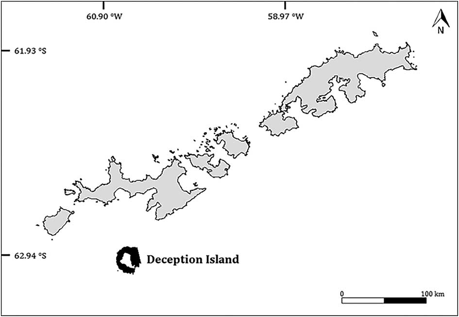
Deception Island (62°57'S, 60°38'W) belongs to the South Shetland Islands archipelago. However, it is located in the Bransfield Strait (Galindo-Zaldívar et al. Reference Galindo-Zaldívar, Jabaloy, Maldonado and Sanz de Galdeano1996, González-Casado et al. Reference González-Casado, Giner-Robles and López-Martínez2000), which divides the archipelago from the Antarctic Peninsula (Baraldo & Rinaldi Reference Baraldo and Rinaldi2000) (Fig. 1). Deception Island is an active volcano and has a horseshoe-shaped morphology, with a c.12 km diameter and a maximum altitude of 539 m at Pond Mount (Molina et al. Reference Molina, de Pablo and Ramos2013). The inner bay of the island (Port Foster) resulted from the collapse of a volcanic chimney (Hawkes Reference Hawkes1961). Port Foster has an almost elliptical shape being 9.8 km long and 5.7 km wide (Smith Reference Smith2003), with an approximate perimeter of 32 km and a maximum mid-bay depth of c. 160 m (Pérez-López et al. Reference Pérez-López, Giner-Robles, Martínez-Díaz, Rodríguez-Pascua, Bejar, Paredes and González-Casado2007). There is a narrow connection between the inner bay and the sea located at the south-east of the island, known as Neptune’s Bellows, which has a maximum depth of c. 10 m.
Location of Deception Island relative to the South Shetland Islands.

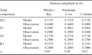
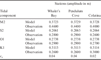
The tide is responsible for diurnal and/or semi-diurnal variability. The main tidal components are the M2, K1, O1 and S2, with M2 of an amplitude of 0.4 m being the most relevant. The other components have amplitudes c. 0.28 m (Lopez et al. Reference Lopez, Garcia, Gomis, Rojas, Sospedra and Sanchez-Arcilla1999). Velocity amplitudes are lower at Port Foster (<0.05 m s-1), and the maximum tidal currents are observed in Neptune’s Bellows ranging between 0.64 and 0.76 m s-1. Tidal heights reach a maximum 3 m during spring tides (Lenn et al. Reference Lenn, Chereskin and Glatts2003). Neptune’s Bellows is also the area where most of the tidal energy is dissipated (Vidal et al. Reference Vidal, Berrocoso and Fernandez-Ros2012).
Orographical constraints in the region have a major influence on the wind. At Bellingshausen Station (located on King George Island, South Shetland Islands) the winds are predominantly from the west and north-west, whereas the winds detected by the Terrestrial Station (located on Deception Island) are predominantly from the north-east and south-west. Using a local WRF model, Comin et al. (unpublished) demonstrated that the winds on Deception Island are predominantly from the north-west and south-east.
According to Lenn et al. (Reference Lenn, Chereskin and Glatts2003), baroclinic tides are generated in Neptune’s Bellows, and the study of these tides is important for understanding water column mixing processes inside Port Foster (Flexas et al. Reference Flexas, Arias and Ojeda2017). Baroclinic tides are internal waves in stratified fluids that result from the interaction of barotropic tides (generated by astronomical forcing) with topography (Levine et al. Reference Levine, Padman, Muench and Morison1997).
Model setup
The 3D numerical hydrodynamic model used in this work was MOHID (Martins et al. Reference Martins, Leitão, Silva and Neves2001), which has been applied in numerous studies since its creation (e.g. Coelho et al. Reference Coelho, Neves, Leitão, Martins and Santos1999, Trancoso et al. Reference Trancoso, Saraiva, Fernandes, Pina, Leitão and Neves2005, Vaz et al. Reference Vaz, Dias, Leitão and Martins2005, Reference Vaz, Mateus, Plecha, Sousa, Leitão, Neves and Dias2015). The numerical computation was carried out on a spatial domain representative of Port Foster and its surroundings using a grid consisting of 40 334 square elements (134 rows and 301 columns); each square has a horizontal resolution of ∆x=∆y=50 m. A Cartesian co-ordinate system was adopted for the vertical resolution (∆z). Parameters related to hydrodynamics include the bottom drag coefficient and the horizontal and vertical eddy viscosities. The value assumed for bottom drag coefficient was 3×10⁻³ and for horizontal viscosity was 3 m s-2 (values were chosen based on a previous study by Vidal et al. Reference Vidal, Berrocoso and Jigena2011). The vertical viscosity was obtained from the General Ocean Turbulence Model, where it was calculated using the dynamic equation for the k-epsilon model. A time step of ∆t=45 s was applied for both baroclinic and barotropic simulations. The simulation periods were 3 months for the Antarctic summer and 1 month for the Antarctic winter (avoiding periods of ice plates).
Bathymetry
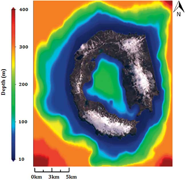
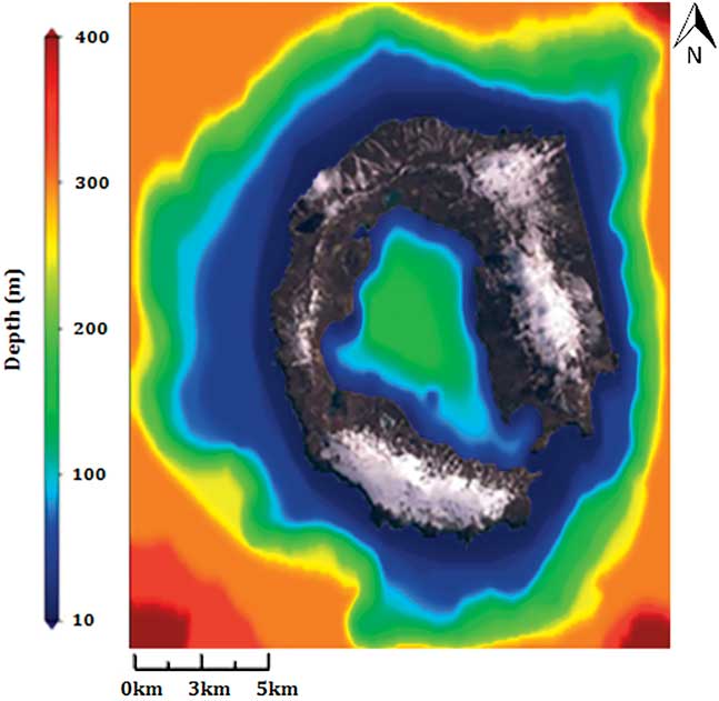
The bathymetry of the bay and the coastline were created using the spatial data infrastructure for Deception Island (SIMAC-IDEDEC), maintained by the Laboratory of Astronomy, Geodesy and Cartography of the University of Cadiz, Spain (Torrecillas et al. Reference Torrecillas, Berrocoso and García-García2006). The outline bathymetry was generated based on a grid from the Autochart Bathymetric Map Production from the National Oceanic and Atmospheric Administration (NOOA). The information was processed using the ArcGIS software and subsequently georeferenced. The resulting bathymetry (Fig. 2) was compared with data from Barclay et al. (Reference Barclay, Wilcock and Ibáñez2009) and found to be similar for the study area. Smoothing was required when merging the two sets of bathymetry data and this was done by linear interpolation for the area outside Neptune’s Bellows.
Modelled domain and bathymetry built from available barometric data.
2D model
In the 2D tidal model, the tide level and phase of the components were imposed as boundary conditions using the FES2004 global tide solution (Lyard et al. Reference Lyard, Lefevre, Letellier and Francis2006), which is the tide level and harmonic predictor of POC-LEGOS, with 14 harmonic components (M2, S2, K1, K2, N2, 2N2, O1, Q1, P1, M4, Mf, Mm, Mtm and MSqm).
The 2D tidal model has been validated by comparing the model results with observational data. The data used is presented in Vidal et al. (Reference Vidal, Berrocoso and Jigena2011) as a result of a harmonic analysis applied to a J number of tidal gauges located on the island. For each constituent of each simulation, the error in the amplitudes
 $$\left( {e_{a} } \right)$$
and phases
 $$\left( {e_{P} } \right)$$
were calculated using:
 $$e_{a} {\equals}\sqrt {{1 \over J}\mathop{\sum}\limits_{i{\equals}1}^J {{{\left( {Ao_{i} {\minus}Am_{i} } \right)^{2} } \over 2}} } , $$
 $$ e_{p} {\equals}{1 \over J}\mathop{\sum}\limits_{i{\equals}1}^J {{{A_{{m_{i} }}^{2} \left( {\theta o_{i} {\minus} \theta m_{i} } \right)} \over {\sum_i A_{{m_{i} }}^{2} }}} .$$
The error in the amplitudes was calculated from the difference between the amplitude observations (Ao) and the results of the model (Am), and the difference in error between the phases
 $$\left( {\theta o_{i} {\minus} \theta m_{i} } \right)$$
, weighted with the values of the model amplitudes (Am). These equations are used to assess the variation between the modelled values and observation data, and were used by Vidal et al. (Reference Vidal, Berrocoso and Jigena2011) in the model setup.
3D model
In the 3D model, T-S profiles were applied with the aim of understanding their role in the current situation. Since there was no reliable data for wind and solar radiation the profiles were made static, i.e. the third term on the right-hand side of Eq. (3) was kept constant:
 $${1 \over {\rho _{0} }}{{\partial p} \over {\partial x_{i} }} {\equals}{1 \over {\rho _{0} }}{{\partial p_{{atm }} } \over {\partial x_{i} }}{\plus}g{{\partial \eta } \over {\partial x_{i} }}{\plus}{g \over {\rho _{0} }}\mathop{\int}\limits_{x_{3} }^\eta {{{\partial \rho ^{'} } \over {\partial x_{i} }}dx_{3} ,} $$
where ρ
0
is the fluid density reference state, x
1 the longitudinal (x
1), transversal (x
2) and vertical distances (x
3), p
atm
the atmospheric pressure, g the gravitational acceleration, η the free surface and
 $$\rho ^{'} $$
the density deviation from the reference state. The pressure term in the horizontal momentum equations is calculated using Eq. (3).
With the lack of reliable wind data, the use of global weather re-analysis was considered but, since the dimensions of the bay are small and the surrounding topography is its major influence, the atmospheric forcing data would be very unreliable.
Locations for the time series outputs
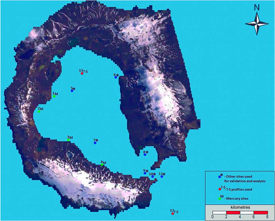
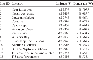
The locations for the time series used in this study were chosen considering the previous tidal data collected, including Neptune’s Bellows and the most relevant sites inside Port Foster (sites 5–11, see Fig. 3). The sites chosen to monitor mercury dispersion (sites 1–4, Fig. 3) were the locations where the most significant mercury samples were collected (de Ferro Reference de Ferro2012). The time series locations and respective site identification numbers are presented in Table I.
Time series locations for model output.

Time series co-ordinates.

Temperature and salinity
The salinity and temperature profiles applied in the model were obtained during the ERUPT III and V expeditions (Smith Reference Smith2003), which occurred during the summer and winter in 2000, respectively. The T-S profiles at site 13 are representative of Port Foster for summer and winter conditions. Site 12 was chosen to represent conditions outside the bay for the summer (Fig. 3) and an additional data point was used to represent T-S profiles outside the bay for winter conditions (63°11'S, 60°32.606'W). These profiles were created based on CTD data provided by Sturz et al. (Reference Sturz, Gray, Dykes, King and Radtke2003). T-S values assigned for outside and inside the bay varied vertically and were assumed to be constant horizontally, except for the interface between the two areas where a linear interpolation was used. Therefore, the density effect over the flow is considered both in stratification (via buoyancy in the vertical turbulence model) and in horizontal pressure gradients.
Residence time and mercury circulation
Considering mercury contamination, since one of the forms in which mercury appears in the marine environment is aggregated to different particles (HgP), an important approach is the residence time, because it gives the average amount of time a particle spends in the bay. The residence time was determined using two approaches. The first approach used:
 $$Tresidence{\,\equals\,}{V \over {Cs{\times}Mf}},$$
where V is the volume of Port Foster (3626 hm3), Mf the mean flow entering Port Foster (1.2 cm s-1), and C S the cross-section at Neptune’s Bellows (5500 m2).
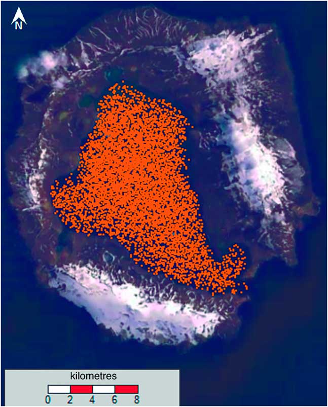
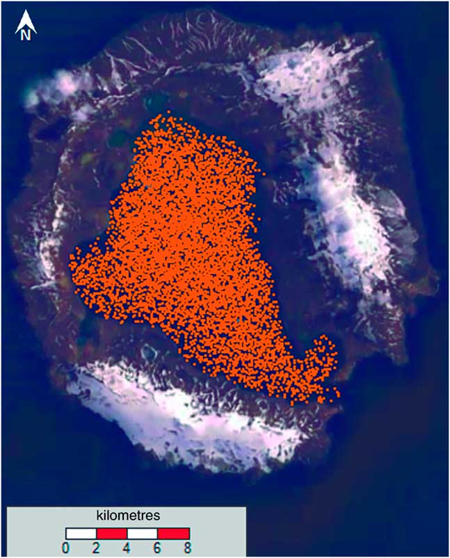
The second approach consisted of filling the bay with Lagrangian tracers (Fig. 4) and completing a 3 month simulation of barotropic conditions to understand the shape of the regression regarding the number of particles leaving the bay over time; this approach follows the practical implementation presented in Murakami (Reference Murakami1991). For the study of mercury circulation, the particles were simulated by using passive Lagrangian tracers, i.e. chemical reactions, such as transformation or particle bounding, were not taken into account. The simulation was performed by releasing particles at a given time and not continuously. This approach was chosen since the authors did not have information on the emission intensity of release. Turbulence parameterization was based on Sullivan Allen formulation. No assumptions were made for the settling velocity of particles to which mercury aggregated; therefore, the model only took into account advection in this simulation.
Bay filled with Lagrangian tracers.
Results
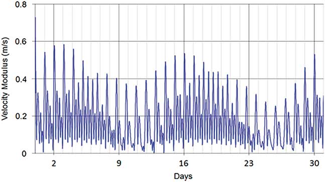
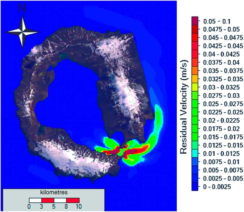
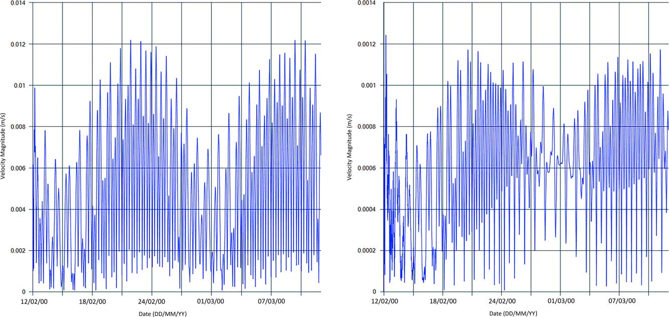
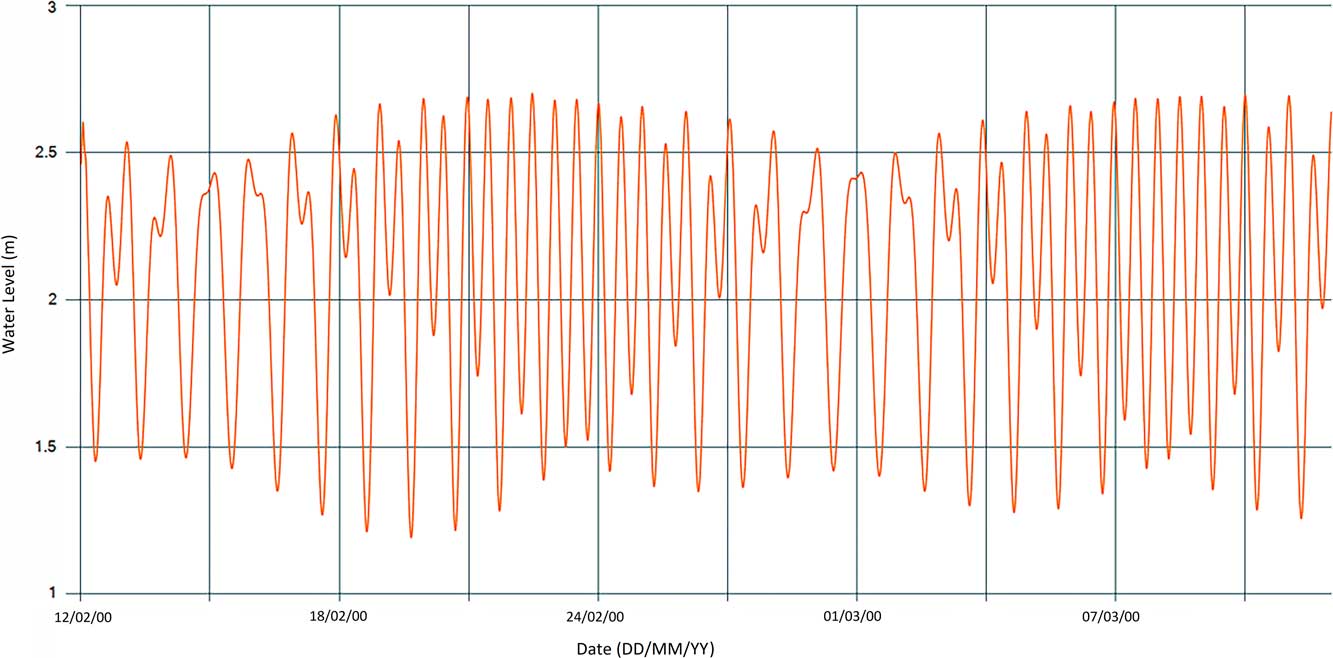
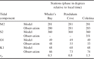
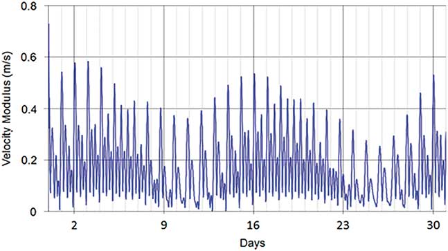
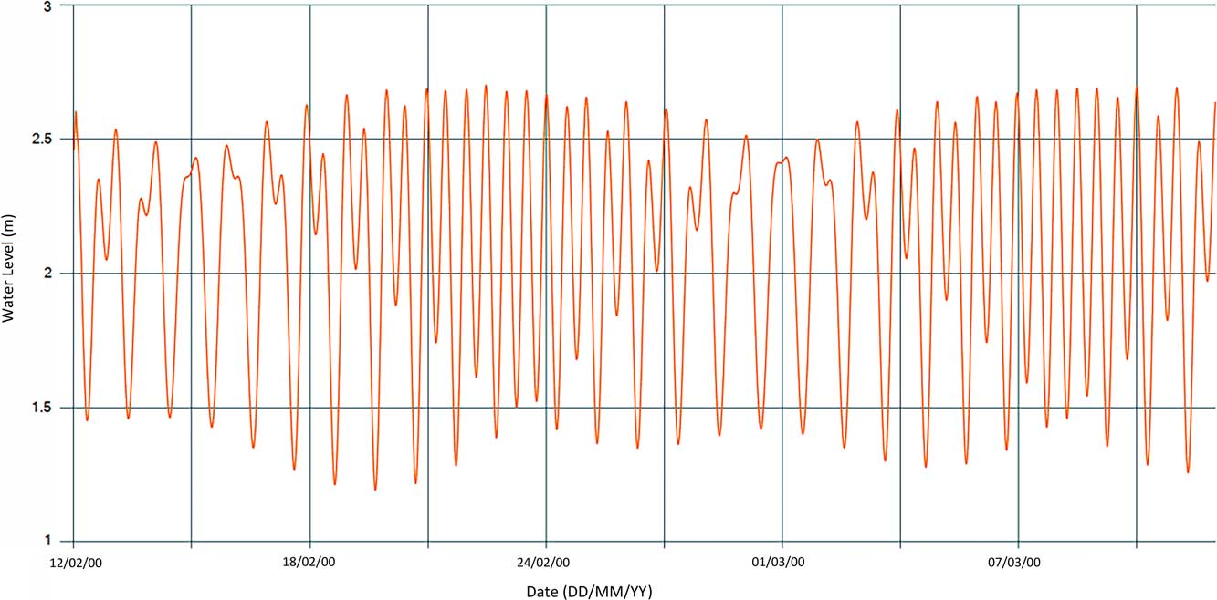
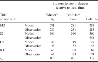
The model results demonstrated that the amplitudes of the velocities in Neptune’s Bellows can reach maximum speeds near 0.60 m s-1 during spring tides (Fig. 5) and the average residual velocity during the simulation was 0.1 m s-1 (Fig. 6). Validation results for amplitude and phase for each tidal constituent used in the simulation are shown in Tables II & III, respectively. Although the predictions for M2 and S2 amplitudes are underestimated, we assume that the results are acceptable for e a (< 0.05 m deviation from the observed data point), taking into account all tidal components. For e p , the results are acceptable, with the model accurately resolving the tidal phase. Model results for surface currents show small velocities (< 0.05 m s-1) at Port Foster (Fig. 7). The velocities near the narrow channel of Neptune’s Bellows also show that the east–west direction is more relevant, in agreement with the orientation of the passage. A mean tidal level variation of 1.2 m can be observed (Fig. 8).
Velocity magnitude in Neptune’s Bellows, 1 month simulation (from 1 July to 1 August 2011).
Model results for the residual velocity after a 1 month simulation period.

Velocity magnitude in two locations: a. Stanley patch (site 7) and b. centre depth (site 5).

Water level at Stanley patch (site 7; 1 month simulation).
Harmonic analysis results for tidal amplitude: model and observation.
Harmonic analysis results for tidal phase: model and observation.
Residence time
The first approach gave a value for residence time of 1.7 years. Whereas the second approach gave a value of c. 70 days. This result comes from an exponential fit (R 2=0.94) between the percentage of initial particles inside the bay (y) and time (x):
 $$y{\equals}98.301e^{{{\minus}7E{\minus}08x}} .$$
With Eq. (5), the residence time was calculated assuming 63% of particles leaving the bay as a good representation.
3D model hydrodynamics
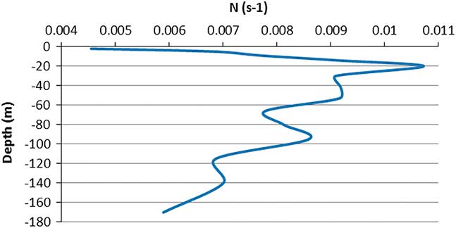
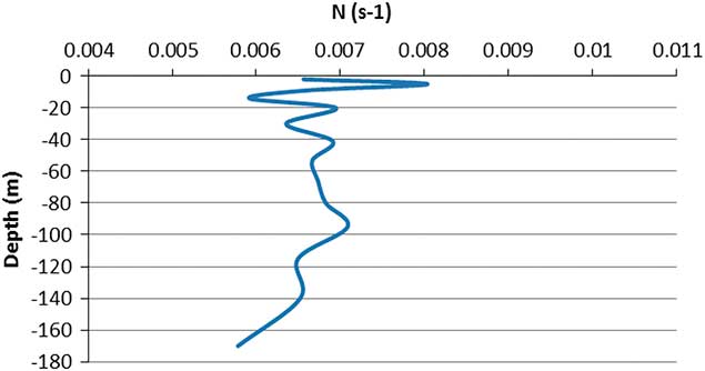
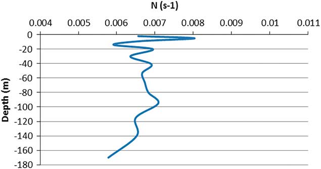
The buoyancy frequency was analysed for summer and winter conditions inside Port Foster. This frequency is related to water column stability and it is a fundamental variable in the dynamics of a stratified flow. The thermocline is located between 10 and 20 m in summer (Fig. 9) and absent in winter when the water column is well mixed (Fig. 10), since the winter simulations were performed during periods of no ice plates. Due to stratification, particles are expected to stay above the thermocline during summer, and in winter, since the water column is well mixed, they are expected to be dispersed over the whole column.
Summer buoyancy frequency at centre depth (site 5).
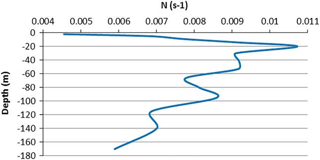
Winter buoyancy frequency at centre depth (site 5).
Internal tides
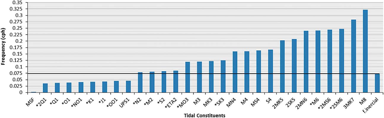
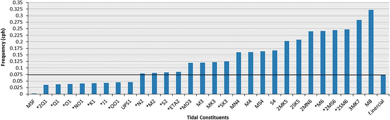
A thorough study of internal tides is outside the scope of this research, which addresses two main issues regarding the generation of baroclinic tides in Neptune’s Bellows: i) in which season (summer or winter) their generation is most likely, and ii) which components of the barotropic tide are more prone to the generation of internal tides. Figure 11 shows the tidal components that can be associated with internal tide generation in Neptune’s Bellows (bars extending above the black line). The frequency band for internal wave propagation ranges between the Coriolis and buoyancy frequency.
Frequency of tidal constituents in Neptune’s Bellows.
The potential sites for generation of internal tides, as well as the more important components related to their appearance, can be deduced from the linear internal wave theory, whereby the bottom slope (bs) is compared with the slope of the internal wave characteristics (c):
 $$c^{2} {\equals}{{w^{2} {\minus}f^{2} } \over {N^{2} {\minus}w^{2} }},$$
where f, N, and w are the inertial, buoyancy and tidal frequencies, respectively.
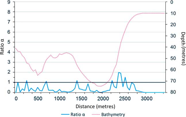
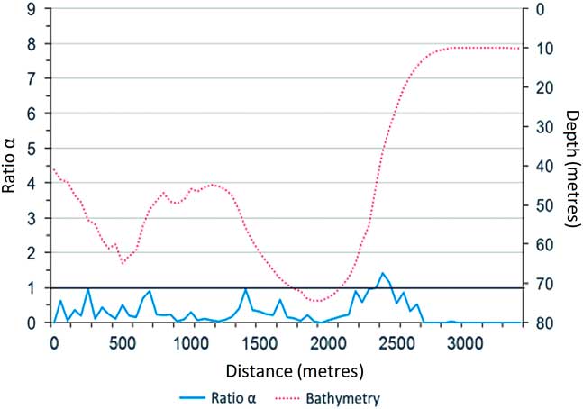
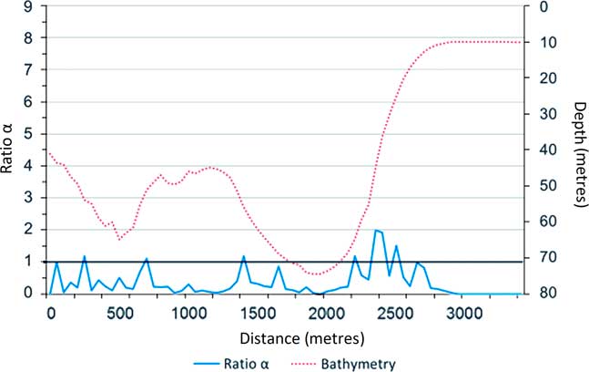
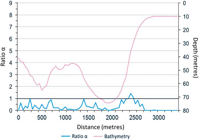
The results for the component M2 in summer and winter are depicted in Figs 12 & 13, respectively.
Summer: alpha ratio for component M2, as a function of depth and distance, from Neptune’s Bellows to inside Port Foster.
Winter: alpha ratio for component M2, as a function of depth and distance, from Neptune’s Bellows to inside Port Foster.
Mercury circulation
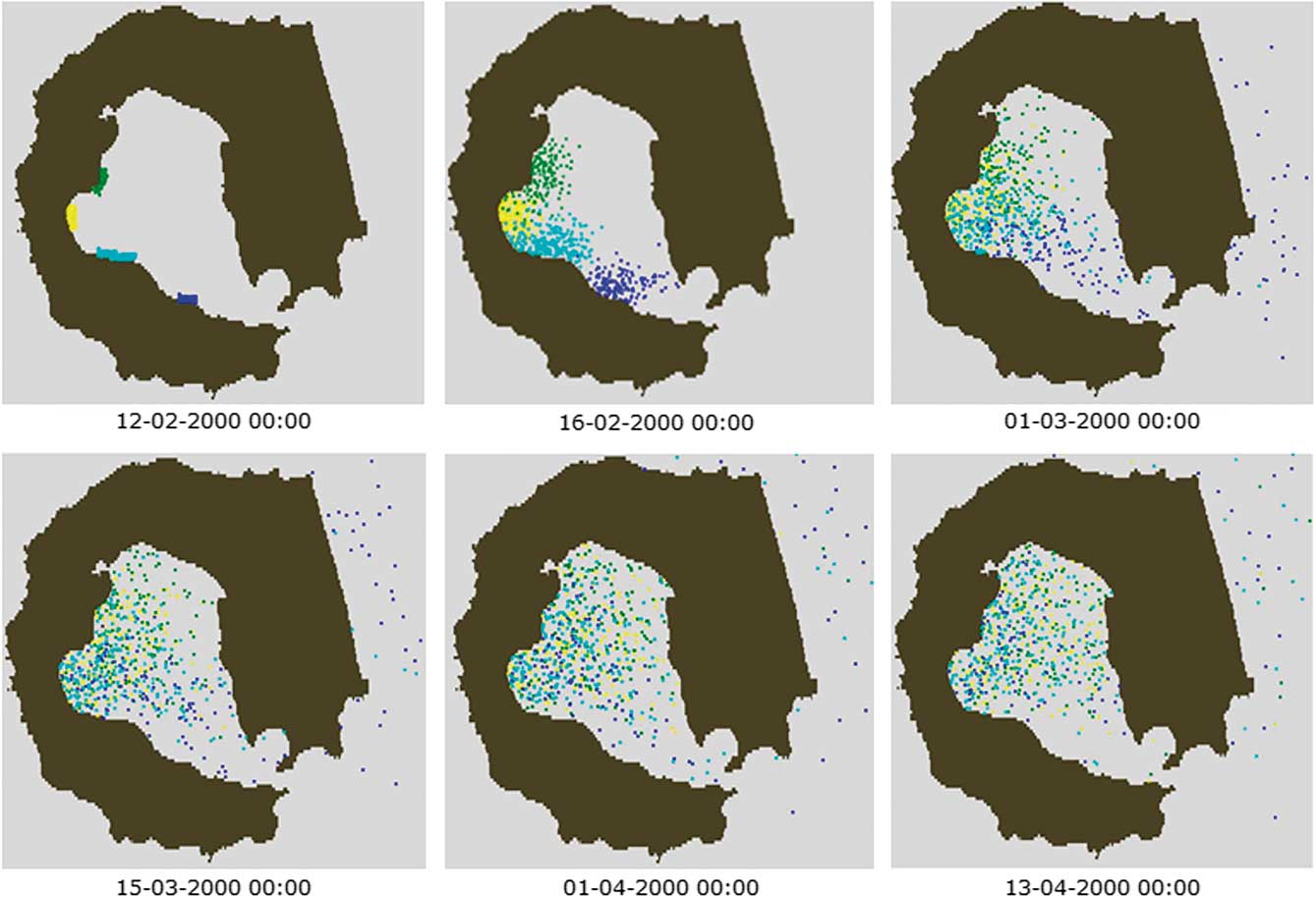
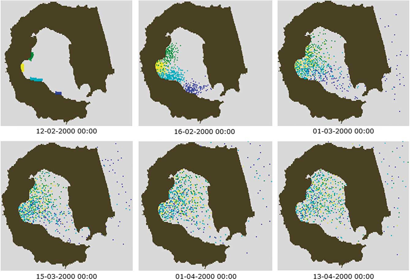
After the 3 month simulation of summer conditions the main conclusions are: i) there is a poor rate of exchange of water between Port Foster and the surrounding areas and ii) the particles tend to accumulate mainly in the western and northern parts of the bay due to the gradual decrease in velocity from Neptune’s Bellows to those regions (Fig. 14).
Lagrangian tracers simulation for summer. Colours represent the location of the initial release of different particles.
Discussion
Surface current and particles accumulation
The model results for surface currents agree with the previous studies of Vidal et al. (Reference Vidal, Berrocoso and Jigena2011) and Lenn et al. (Reference Lenn, Chereskin and Glatts2003). Overall, taking into account all tidal components, the tide in Port Foster was adequately reproduced in the model, despite underestimating M2 and S2 amplitudes; therefore, the tidal model can be applied with confidence. The residence time estimated by empirical formulae (1.7 years) is close to previous estimates reported by Lenn et al. (Reference Lenn, Chereskin and Glatts2003) of 2.4 years based on a mean flow entering Port Foster of 1 cm s-1. However, the value reached by the Lagrangian tracers approach (150 days) is considerably lower. This latter result is highly influenced by the number of particles released and by the simulation period. Despite the uncertainty associated with both methods, we can conclude that the bay is propitious for the accumulation of heavy metals.
Internal waves and mercury circulation
Using the approach proposed by Baines (Reference Baines1982) and Craig (Reference Craig1987) for linear internal wave theory, it can be concluded that baroclinic tides, with the M2 frequency (Figs 12 & 13), can indeed be formed in both summer and winter, and are most likely to propagate in an offshore direction since α>1 (Pereira & Castro Reference Pereira and Castro2007).
The main conclusion for mercury circulation is that particles tend to accumulate in the northern and western areas of the bay and dispersal is relatively slow, reinforcing the prediction of long residence time.
Conclusions
The tidal model was successfully validated and the 2D hydrodynamic model confirmed established circulation patterns at Deception Island, namely, the residual circulation inside Port Foster, variations in sea level and the particle residence time. A 3D simulation was performed and, to the best of our knowledge, this is the first attempt at such an analysis. The 3D model used in this work assumes a steady fluid stratification because there is a lack of data regarding solar radiation and wind forcing. The absence of data implied that the 3D model could not be validated, limiting its ability to make predictions and allow transport process studies. Stratification plays a bigger role in the summer, and there is strong evidence of the generation of internal waves in Neptune’s Bellows in both seasons. The impact of the energy released during this process in Port Foster’s water column is yet to be assessed. The M2 is the main tidal component related to this phenomenon. Another important finding of the model is that Port Foster presents conditions that favour a long residence time. These results, together with similar findings from previous studies, prove that mercury accumulation is occurring in Port Foster; therefore, there is a possible threat to the local ecosystem.
Future studies should focus on the importance of internal tides in transport processes in Port Foster and aim to develop a more complex 3D model that includes meteorological conditions, such as wind stress and radiation, as well as the processes involved in water solidification and ice fusion. For wind stress, the best approach is to create a local scale atmospheric model that is able to describe the microscale physics and account for the orography around Port Foster. The residence time should be simulated again when a more complex 3D model becomes available.
Author contribution
DF, AdS and MM designed the case study. DF gathered the data and created the 2D and the approach to the 3D model with regular help from MM and LP. Data analysis was performed by DF in close co-operation with AdS and all the results of this analysis were reviewed by MM and LP. The simulations were performed by DF and both MM and LP ensured quality on this modelling step. DF was the lead writer of the manuscript and all authors contributed to its revision and final structure.