2.1. Design of the 3UPS–3SS parallel mechanism

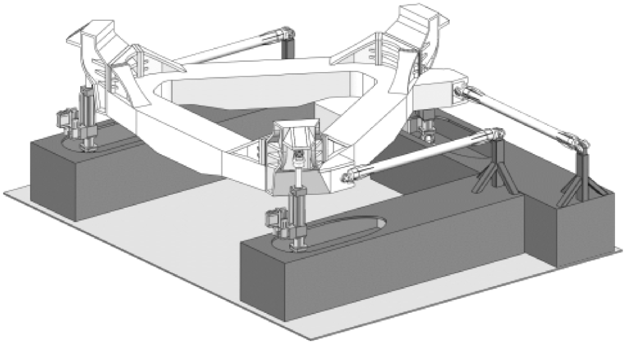
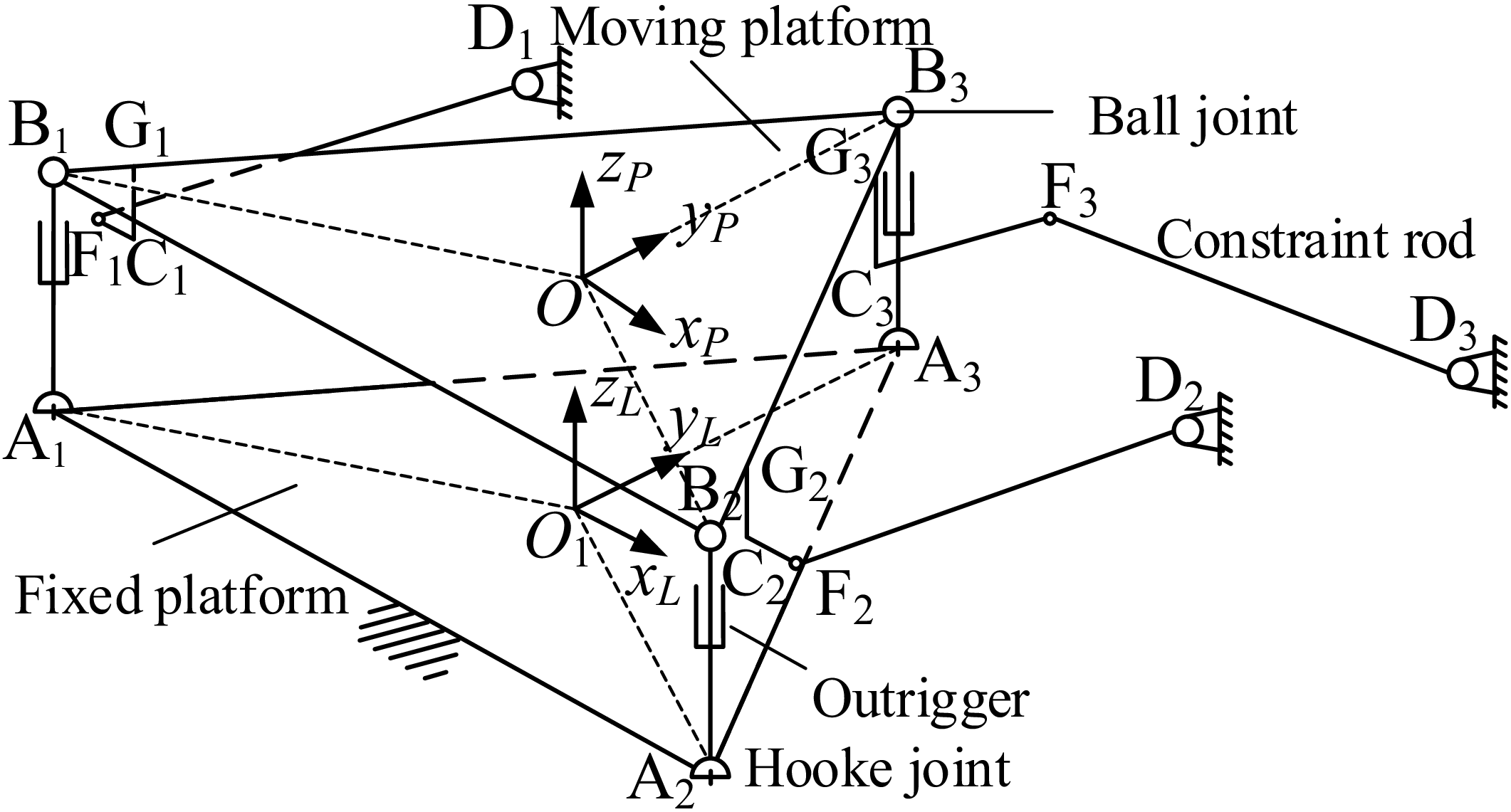
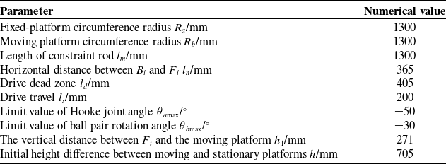
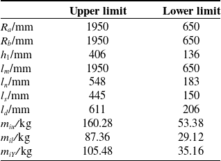
Figures 1 and 2, respectively, show the three-dimensional model of the initial position and the schematic diagram of the 3UPS-3SS parallel mechanism. The mechanism consists of a moving platform, a fixed platform, 3 driving branches, and 3 constraint branches. The fixed platform is fixed on the hull. The 3 driving branches, A _i B _i (i = 1, 2, 3 in the following text), connect the moving platform and the fixed platform, which are UPS configurations. The driving element of the driving branch is a hydraulic drive unit (P pair). Its connecting part on the fixed-platform end is a universal pair (U pair), and the connecting part on the moving platform end is a spherical pair (S pair). The length of the driving rod A _i B _i is l _i , and the initial length of A _i B _i is the initial height difference h between the moving platform and the fixed platform. The two ends of the 3 equal-length constraint rods, F _i D _i , are respectively connected to the moving platform and the fixed platform through spherical pairs (S pairs), which are the constraint branches of the SS configuration. The hinge point F _i is located at h ₁ below the moving platform, that is, |C _i G _i | = h ₁.

Figure 1.

3D model of 3UPS-3SS parallel mechanism.

Figure 1. Long description

A 3D model of a 3UPS-3SS parallel mechanism, showcasing its high rigidity, high speed, and large load capacity. The mechanism features a complex structure with multiple interconnected components, including triangular platforms connected by struts and spherical joints. The design emphasizes precise adaptation to specific task requirements, such as attitude adjustment and wave compensation. The model highlights the innovative layout of the branch chains to improve workspace isotropy, making it suitable for industrial manufacturing, aerospace, and ocean engineering applications.

Figure 2.

Schematic diagram of 3UPS-3SS parallel mechanism.

Figure 2. Long description

The schematic diagram of a 3UPS-3SS parallel mechanism features a fixed platform and a moving platform connected by three identical branches. Each branch consists of a universal joint (U) connected to a prismatic joint (P) and then to a spherical joint (S). The fixed platform is labeled with points A1 and A2, while the moving platform is labeled with points B1, B2, and B3. Constraint rods connect points B3, C3, and D3, forming a triangular structure. The diagram includes axes labeled xP, yP, zP for the moving platform and xL, yL, zL for the local coordinate system. Ball joints, constraint rods, and outriggers are also labeled, showing their connections and interactions within the mechanism.

As shown in Figure 2, a fixed coordinate system O ₁ x _L y _L z _L (denoted as {L}) is established on the fixed platform. The positive directions of the x _L axis and y _L axis are along the directions of A ₁ A ₂ and O ₁ A ₃ , respectively, and the z _L axis is perpendicular to the fixed platform. A moving coordinate system Ox _P y _P z _P (denoted as {P}) is established on the moving platform. The positive directions of the x _P axis and y _P axis are along the directions of B ₁ B ₂ and OB ₃ , respectively, and the z _P axis is perpendicular to the moving platform.

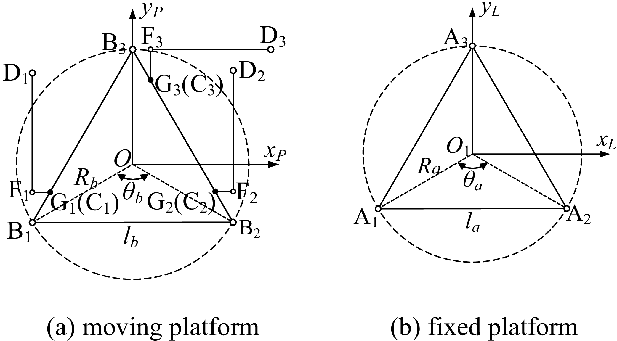
The hinge point where the driving rods connect to the fixed platform is A _i , and that connecting to the moving platform is B _i . As shown in Figure 3, the hinge point A _i forms an equilateral triangle, which is inscribed in a circle with radius R _a , with the center at O ₁ , and the central angle corresponding to each side of the triangle is $\theta$ _a . The hinge point B _i forms an equilateral triangle, which is inscribed in a circle with radius R _b , with the center at O, and the central angle corresponding to each side of the triangle is $\theta$ _b , where $\theta$ _a = $\theta$ _b . The characteristic of this mechanism is that when it is in the initial position, the moving platform is parallel to the fixed platform, the origin O ₁ of the fixed coordinate system is the projection of the center O of the moving platform onto the fixed platform, the axis of the driving rod is perpendicular to the fixed platform, and the 3 constraint rods are in a plane parallel to the fixed platform. From the viewing angle shown in Figure 3, B, F, and D are collinear; besides, |B _i F _i | = l _{n and} |F _i D _i | = l _m .

Figure 3.

Schematic diagram of moving platform and fixed-platform structure.

Figure 3. Long description

The image presents a schematic diagram of a moving platform and a fixed-platform structure. The moving platform, labeled as (a), features a triangular arrangement with points B1, B2, and B3 connected to points F1, F2, and F3 respectively. The fixed platform, labeled as (b), also has a triangular arrangement with points A1, A2, and A3. Both platforms include central points O and O1, with radii Rb and Ra extending to their respective vertices. The moving platform includes angles θb and distances lb, while the fixed platform includes angle θa and distance la. The diagram illustrates the geometric relationships and configurations of these platforms, highlighting their structural design and key points.

2.2. Degree-of-freedom analysis of the 3UPS-3SS parallel mechanism based on screw theory

In this section, screw theory is applied to analyze the degrees of freedom (DOF) of the mechanism, and the modified G–K equation is used to validate the DOF calculation:

(1) \begin{equation} F=d\left(n-g-1\right)+\mathop{\sum }\limits_{i=1}^{g}f_{i}+v-\zeta \end{equation}

where F – DOF of the mechanism. d – order of the mechanism. n – total number of links in the mechanism. g – number of kinematic pairs in the mechanism. f _i – degrees of freedom of the i-th kinematic pair. v – redundant degrees of freedom of the mechanism. $\zeta$ – local degrees of freedom of the mechanism.

The coordinates of the kinematic pairs at points A ₁, A ₂, and A ₃ are defined as follows:

(2) \begin{equation} \begin{array}{l@{\quad}l@{\quad}l} s_{1,1}=\left[\begin{array}{l@{\quad}l@{\quad}l} -\dfrac{\sqrt{3}}{2}R_{a} & -\dfrac{1}{2}R_{a} & 0 \end{array}\!\right] & s_{1,2}=\left[\begin{array}{l@{\quad}l@{\quad}l} \dfrac{\sqrt{3}}{2}R_{a} & -\dfrac{1}{2}R_{a} & 0 \end{array}\!\right] & s_{1,3}=\left[\begin{array}{l@{\quad}l@{\quad}l} 0 & R_{a} & 0 \end{array}\!\right] \end{array} \end{equation}

The coordinates of the kinematic pairs at points B ₁, B ₂, and B ₃ are defined as follows:

(3) \begin{equation} \begin{array}{l@{\quad}l@{\quad}l} s_{2,1}=\left[\begin{array}{l@{\quad}l@{\quad}l} -\dfrac{\sqrt{3}}{2}R_{b} & -\dfrac{1}{2}R_{b} & h \end{array}\!\right] & s_{2,2}=\left[\begin{array}{l@{\quad}l@{\quad}l} \dfrac{\sqrt{3}}{2}R_{b} & -\dfrac{1}{2}R_{b} & h \end{array}\!\right] & s_{2,3}=\left[\begin{array}{l@{\quad}l@{\quad}l} 0 & R_{b} & h \end{array}\!\right] \end{array} \end{equation}

The coordinates of the kinematic pairs at points F ₁, F ₂, and F ₃ are defined as follows:

(4) \begin{equation} \begin{array}{l@{\quad}l@{\quad}l} s_{3,1}=\left[\begin{array}{l@{\quad}l@{\quad}l} -\dfrac{\sqrt{3}}{2}R_{b} & l_{n}-\dfrac{1}{2}R_{b} & h-h_{1} \end{array}\!\right] & s_{3,2}=\left[\begin{array}{l@{\quad}l@{\quad}l} \dfrac{\sqrt{3}}{2}R_{b} & l_{n}-\dfrac{1}{2}R_{b} & h-h_{1} \end{array}\!\right] & s_{3,3}=\left[\begin{array}{l@{\quad}l@{\quad}l} l_{n} & R_{b} & h-h_{1} \end{array}\!\right] \end{array} \end{equation}

The coordinates of the kinematic pairs at points D ₁, D ₂, and D ₃ are defined as follows:

(5) \begin{align} & \begin{array}{l@{\quad}l@{\quad}l} s_{4,1}=\left[\begin{array}{l@{\quad}l@{\quad}l} -\dfrac{\sqrt{3}}{2}R_{b} & l_{m}+l_{n}-\dfrac{1}{2}R_{b} & h-h_{1} \end{array}\!\right] & s_{4,2}=\left[\begin{array}{l@{\quad}l@{\quad}l} \dfrac{\sqrt{3}}{2}R_{b} & l_{m}+l_{n}-\dfrac{1}{2}R_{b} & h-h_{1} \end{array}\!\right] & \end{array}\nonumber \\&\; s_{4,3}=[\begin{array}{l@{\quad}l@{\quad}l} l_{m}+l_{n} & R_{b} & h-h_{1} \end{array}] \end{align}

Thus, in the initial configuration, the motion screw system of the SS can be expressed as follows:

(6)

(7)

(8)

The results are defined as follows:

(9)

(10)

(11)

According to the principle of reciprocal screws, (1) two line vectors are reciprocal if and only if they are coplanar. If they are not coplanar, they cannot be reciprocal. (2) Two moments are always reciprocal. (3) A line vector and a moment are reciprocal only when they are perpendicular. If they are not perpendicular, they are not reciprocal. (4) Both line vectors and moments are self-reciprocal.

Through in-depth analysis of the 3UPS drive branch chains and the 3SS constraint branch chains, the following conclusions can be drawn: the 3SS structure part contains three reciprocal screws, while the 3UPS structure part has no counter-rotating quantity characteristics. Therefore, the three counter-rotating quantities of the 3SS constraint branch chain pairwise constitute the overall counter-rotating quantity system of the 3UPS-3SS mechanism, and the corresponding constraint rotational quantity is shown as follows

(12) \begin{align} \begin{array}{l} {S}_{1}^{r}=\left[\begin{array}{l@{\quad}l@{\quad}l@{\quad}l@{\quad}l@{\quad}l@{\quad}l} 0 & 1 & 0 & ; & -h & 0 & \dfrac{\sqrt{3}}{2}R_{b} \end{array}\!\right]^{T}\\[10pt] {S}_{2}^{r}=\left[\begin{array}{l@{\quad}l@{\quad}l@{\quad}l@{\quad}l@{\quad}l@{\quad}l} 0 & 1 & 0 & ; & -h & 0 & \dfrac{\sqrt{3}}{2}R_{b} \end{array}\!\right]^{T}\\[10pt] {S}_{3}^{r}=\left[\begin{array}{l@{\quad}l@{\quad}l@{\quad}l@{\quad}l@{\quad}l@{\quad}l} 1 & 0 & 0 & ; & 0 & h & R_{b} \end{array}\!\right]^{T} \end{array} \end{align}

Thus, the constraint screw system of the 3UPS-3SS parallel mechanism is given by:

(13)

where f is the eccentricity in the constrained rotation, which is used to describe the offset influence of the torque transmission direction and magnitude relative to the coordinate origin.

Based on screw reciprocity, the motion screw system of the 3UPS-3SS parallel mechanism is given by:

(14)

Based on the calculation, the mechanism has three degrees of freedom, the translation O _z along the axis z _L and the rotation ( $\theta$ _x = $\gamma$ and $\theta$ _y = $\beta$ ) around the axes x _L and y _L , so the motion mode of the parallel stabilization platform is 2R1T.

The correctness of this DOF analysis is further validated using the modified G–K equation, as follows:

(15) \begin{equation} F=d\left(n-g-1\right)+\mathop{\sum }\limits_{i=1}^{g}f_{i}+v-\zeta =6\left(13-15-1\right)+36+0-0=3 \end{equation}

3.1. Inverse solution on position

By defining the transformation matrix R through the Roll-Pitch-Yaw angle (RPY), describe the rotation of the dynamic coordinate system {P} relative to the fixed coordinate system {L}: first rotate around the x _L axis of {L} by $\gamma$ , then around the y _L axis by $\beta$ , and finally around the z _L axis by $\alpha$ , then the rotation matrix is:

(16) \begin{equation} \begin{array}{l} {\boldsymbol{R}}={\boldsymbol{R}}(z,\alpha ){\boldsymbol{R}}(y,\beta ){\boldsymbol{R}}(x,\gamma )\\[5pt] =\left[\begin{array}{c@{\quad}c@{\quad}c} \cos \alpha \cos \beta & \mathit{\cos }\mathit{\alpha }\sin \beta \sin \gamma -\sin \alpha \cos \gamma & \mathit{\cos }\mathit{\alpha }\sin \beta \cos \gamma +\sin \alpha \sin \gamma \\[5pt] \sin \alpha \sin \beta & \mathit{\sin }\mathit{\alpha }\sin \beta \sin \gamma +\cos \alpha \cos \gamma & \mathit{\sin }\mathit{\alpha }\sin \beta \cos \gamma -\cos \alpha \sin \gamma \\[5pt] -\sin \beta & \cos \beta \sin \gamma & \cos \beta \cos \gamma \end{array}\!\right] \end{array} \end{equation}

The position vector of the subcenter point A _i of the U pair of the fixed platform at {L} is:

(17) \begin{equation} {}^{L}{{\boldsymbol{A}}}{_{i}^{}}=(\begin{array}{l@{\quad}l@{\quad}l} A_{ix} & A_{iy} & A_{iz} \end{array})^{\mathrm{T}} \end{equation}

The position vector of the center position B _i of the ball pair of the S pair of the moving platform at {P} is:

(18) \begin{equation} {}^{P}{{\boldsymbol{B}}}{_{i}^{}}=(\begin{array}{l@{\quad}l@{\quad}l} B_{ix} & B_{iy} & B_{iz} \end{array})^{\mathrm{T}} \end{equation}

The position vector of the origin O of the moving coordinate system at {P} in {L} is:

(19) \begin{equation} {}^{L}{{\boldsymbol{O}}}{_{P}^{}}=(\begin{array}{l@{\quad}l@{\quad}l} {}^{L}{O}{_{Px}^{}} & {}^{L}{O}{_{Py}^{}} & {}^{L}{O}{_{Pz}^{}} \end{array})^{\mathrm{T}} \end{equation}

Then the position vector of hinge point B _i at {L} is:

(20) \begin{equation} {}^{L}{{\boldsymbol{B}}}{_{i}^{}}={}^{L}{{\boldsymbol{O}}}{_{P}^{}}+{\boldsymbol{R}}{}^{P}{{\boldsymbol{B}}}{_{i}^{}} \end{equation}

The position vector of the ball pair point F _i of the constraint branch on the moving platform at {P} is:

(21) \begin{equation} {}^{P}{{\boldsymbol{F}}}{_{i}^{}}=(\begin{array}{l@{\quad}l@{\quad}l} F_{ix} & F_{iy} & F_{iz} \end{array})^{\mathrm{T}} \end{equation}

Then the position vector of F _i under {L} is:

(22) \begin{equation} {}^{L}{{\boldsymbol{F}}}{_{i}^{}}={}^{L}{{\boldsymbol{O}}}{_{P}^{}}+{\boldsymbol{R}}{}^{P}{{\boldsymbol{F}}}{_{i}^{}} \end{equation}

The position vector of the ball pair point D _i of the constraint branch on the fixed platform at {L} is:

(23) \begin{equation} {}^{L}{{\boldsymbol{D}}}{_{i}^{}}=(\begin{array}{l@{\quad}l@{\quad}l} D_{ix} & D_{iy} & D_{iz} \end{array})^{\mathrm{T}} \end{equation}

The constraint equations for the three constraint rods are:

(24) \begin{align} \begin{cases} (D_{1x}-F_{1x})^{2}+(D_{1y}-F_{1y})^{2}+(D_{1z}-F_{1z})^{2}={l}_{m}^{2}\\[5pt] (D_{2x}-F_{2x})^{2}+(D_{2y}-F_{2y})^{2}+(D_{2z}-F_{2z})^{2}={l}_{m}^{2}\\[5pt] (D_{3x}-F_{3x})^{2}+(D_{3y}-F_{3y})^{2}+(D_{3z}-F_{3z})^{2}={l}_{m}^{2} \end{cases} \end{align}

The length vector of the i-th driving rod of the mechanism is l _i , which can be calculated from the center position ^L B _i of the ball pair and the center position ^L A _i of the Hooke pair of the i-th driving branch in the fixed coordinate system {L}, as shown in the following equation:

(25) \begin{equation} {\boldsymbol{l}}_{i}={}^{L}{{\boldsymbol{B}}}{_{i}^{}}-{}^{L}{{\boldsymbol{A}}}{_{i}^{}} \end{equation}

Combining Eqs. (20) and (25) to obtain:

(26) \begin{equation} {\boldsymbol{l}}_{i}={}^{L}{{\boldsymbol{O}}}{_{P}^{}}+{\boldsymbol{R}}{}^{P}{{\boldsymbol{B}}}{_{i}^{}}-{}^{L}{{\boldsymbol{A}}}{_{i}^{}} \end{equation}

Then the length of the mechanism drive rod is:

(27) \begin{equation} \left| {\boldsymbol{l}}_{i}\right| =\sqrt{{l}_{1}^{2}+{l}_{2}^{2}+{l}_{3}^{2}} \end{equation}

where l ₁, l ₂, and l ₃ are respectively the actual lengths of the driving rod in the x, y, and z directions.

The theoretical length L _i of the mechanism drive rod is:

(28) \begin{equation} L_{i}=\sqrt{(B_{i}-A_{i})^{\mathrm{T}}(B_{i}-A_{i})} \end{equation}

Using the least squares method, an objective function is established to solve the length of the driving rod:

(29) \begin{equation} F(x,y,z,\theta _{x},\theta _{y},\theta _{z})=\mathop{\sum }\limits_{i=1}^{3}[l_{i}-L_{i}]^{2} \end{equation}

where (x, y, z, $\theta$ _x , $\theta$ _y , and $\theta$ _z ) is the pose of the driving rod in the fixed coordinate system {L}. $\theta$ _x , $\theta$ _y , and $\theta$ _z are, respectively, the rotation angles of the driving rod around the x _L , y _L , and z _L axes.

3.2. Inverse solution on velocity

This section focuses on analyzing the velocity characteristics of the moving parts of the shipborne stable platform, emphasizing both linear and angular velocities. Firstly, through theoretical calculations and mathematical modeling, the linear velocity distribution of each moving component is determined. The angular velocity characteristics are then explored in detail, based on the principles of rigid body kinematics.

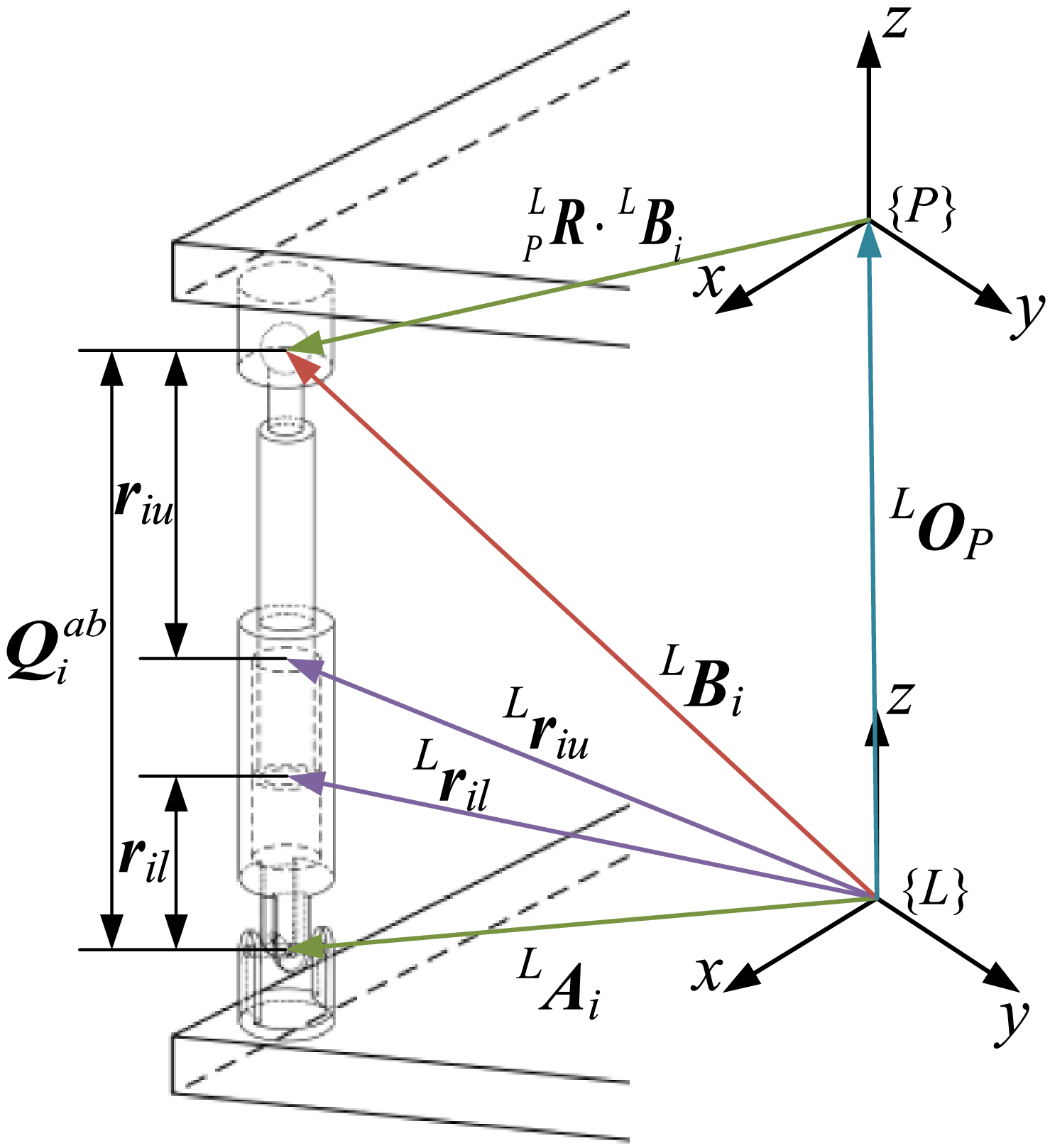
The position information and size parameters of the i-th driving branch in the stabilization platform are shown in Figure 4. By performing derivative operations on both sides of the inverse kinematics equation, the velocity model of the parallel mechanism is obtained.

Figure 4.

Stabilize the position and size parameters of the i-th drive branch of the platform.

Figure 4. Long description

The diagram illustrates a mechanical system with a cylindrical structure and various labeled components. The system includes points labeled as L A i, L B i, L r i u, and L r i l, with corresponding vectors and distances. Two coordinate systems, {L} and {P}, are shown with axes labeled x, y, and z. The diagram also features a point Q i a b and vectors such as L R dot L B i and L O P. The relationships between these components are depicted through lines and arrows, indicating their spatial and functional connections.

The center of mass of the moving platform of this institution is ^P E _up at {P} and ^L E _up at {L}, which can be expressed as:

(30) \begin{equation} {}^{L}{{\boldsymbol{E}}}{_{up}^{}}={}^{L}{{\boldsymbol{O}}}{_{P}^{}}+{}_{P}^{L}{{\boldsymbol{R}}}{}{}^{P}{{\boldsymbol{E}}}{_{up}^{}} \end{equation}

The position of the parallel stabilization platform driving branch UPS pair at {L} is ${}^{L}{{Q}_{i}^{ab}}{}$ ,which can be expressed as:

(31) \begin{equation} {}^{L}{{\boldsymbol{Q}}}{_{i}^{ab}}={}^{L}{{\boldsymbol{O}}}{_{P}^{}}+{}_{P}^{L}{{\boldsymbol{R}}}{_{}^{P}}{\boldsymbol{B}}_{i}-{}^{L}{{\boldsymbol{A}}}{_{i}^{}} \end{equation}

The position of the fixed-length constrained branched SS pair at {L} is ${}^{L}{{Q}_{i}^{cd}}{}$ ,which can be expressed as:

(32) \begin{equation} {}^{L}{{\boldsymbol{Q}}}{_{i}^{cd}}={}^{L}{{\boldsymbol{O}}}{_{P}^{}}+{}_{P}^{L}{{\boldsymbol{R}}}{_{}^{P}}{\boldsymbol{F}}_{i}-{}^{L}{{\boldsymbol{D}}}{_{i}^{}} \end{equation}

The positions of the piston center of mass and cylinder center of mass of the i-th drive branch UPS pair at {L} are ^L r _iu and ^L r _il , respectively, which can be expressed as:

(33) \begin{equation} {}^{L}{{\boldsymbol{r}}}{_{iu}^{}}={}^{L}{{\boldsymbol{A}}}{_{i}^{}}-\left({Q}_{i}^{ab}-r_{iu}\right){}^{L}{\hat{{\boldsymbol{Q}}}}{_{i}^{ab}} \end{equation}

(34) \begin{equation} {}^{L}{{\boldsymbol{r}}}{_{il}^{}}={}^{L}{{\boldsymbol{A}}}{_{i}^{}}+r_{il}{}^{L}{\hat{{\boldsymbol{Q}}}}{_{i}^{ab}} \end{equation}

where ${}^{L}{{\hat{Q}}_{i}^{cd}}{}$ is the unit directional vector of the i-th drive branch UPS pair. ${Q}_{i}^{ab}$ is the length of the i-th drive branch UPS pair.

In the coordinate system {L}, the centroid position of the i-th fixed-length constraint branch SS can be represented as ^L r _iY , and its mathematical expression is:

(35) \begin{equation} {}^{L}{{\boldsymbol{r}}}{_{iY}^{}}={}^{L}{{\boldsymbol{A}}}{_{i}^{}}+r_{iY}{}^{L}{\hat{{\boldsymbol{Q}}}}{_{i}^{cd}} \end{equation}

where ${}^{L}{{\hat{Q}}_{i}^{cd}}{}$ is the unit direction vector of the fixed-length constrained branch SS.

The velocity of the center of mass of the moving platform of the shipborne stabilization platform in the coordinate system {L} can be obtained by performing a time differentiation on both sides of Eq. (30), and its mathematical expression is:

(36) \begin{equation} {}^{L}{\dot{{\boldsymbol{E}}}}{_{up}^{}}={}^{L}{\dot{{\boldsymbol{O}}}}{_{P}^{}}+{}_{P}^{L}{\boldsymbol{\omega }}{}\times {}_{P}^{L}{{\boldsymbol{R}}}{_{}^{P}}{\boldsymbol{E}}_{up} \end{equation}

where ${}_{P}^{L}{\boldsymbol{\omega }}{}$ is the angular velocity of {P} relative to {L}.

The velocity of the hinge point B _i of the driving branch on the moving platform at {L} is obtained by differentiating the first-order time on both sides of Eq. (20):

(37) \begin{equation} {}^{L}{\dot{{\boldsymbol{B}}}}{_{i}^{}}={}^{L}{\dot{{\boldsymbol{O}}}}{_{P}^{}}+{}_{P}^{L}{\boldsymbol{\omega }}{}\times {}_{P}^{L}{{\boldsymbol{R}}}{_{}^{P}}{\boldsymbol{B}}_{i} \end{equation}

The velocity of the hinge point B _i of the driving branch on the moving platform at {L} is also the velocity of B _i relative to A _i , which is:

(38) \begin{equation} {}^{L}{\dot{{\boldsymbol{B}}}}{_{i}^{}}={}^{L}{\dot{{\boldsymbol{Q}}}}{_{i}^{ab}} \end{equation}

The velocity of the driving branch UPS pair at {L} is obtained by differentiating the first-order time on both sides of Eq. (31) simultaneously:

(39) \begin{equation} {}^{L}{\dot{{\boldsymbol{Q}}}}{_{i}^{ab}}={\dot{Q}}_{i}^{ab}\;{}^{L}{\hat{{\boldsymbol{Q}}}}{_{i}^{ab}}+{Q}_{i}^{ab}\;{}_{G_i}^{L}{\boldsymbol{\omega }}{}\times {}^{L}{\hat{{\boldsymbol{Q}}}}{_{i}^{ab}} \end{equation}

where ${Gi}^{L}{\omega }{}$ is the angular velocity of the i-th drive branch UPS pair at {L}.

The velocity of the constrained pair of the moving platform at {L} is obtained by simultaneously differentiating the first-order time on both sides of Eq. (22):

(40) \begin{equation} {}^{L}{\dot{{\boldsymbol{F}}}}{_{i}^{}}={}^{L}{\dot{{\boldsymbol{O}}}}{_{P}^{}}+{}_{P}^{L}{\boldsymbol{\omega }}{}\times {}_{P}^{L}{{\boldsymbol{R}}}{_{}^{P}}{\boldsymbol{F}}_{i} \end{equation}

Similarly, from Eq. (32), the velocity of the fixed-platform constrained pair at {L} can be obtained as follows:

(41) \begin{equation} {}^{L}{\dot{{\boldsymbol{D}}}}{_{i}^{}}={}^{L}{\dot{{\boldsymbol{Q}}}}{_{i}^{cd}}={\dot{Q}}_{i}^{cd}\;\;{}^{L}{\hat{{\boldsymbol{Q}}}}{_{i}^{cd}}+{Q}_{i}^{cd}{}_{Yi}^{{\,}{L}}{\boldsymbol{\omega }}{}\times {}^{L}{\hat{{\boldsymbol{Q}}}}{_{i}^{cd}} \end{equation}

The velocity of the center of mass of the piston of the UPS pair in the i-th driving branch at {L} is obtained by differentiating both sides of Eq. (33) with respect to time in the first order

(42) \begin{equation} {}^{L}{\dot{{\boldsymbol{r}}}}{_{iu}^{}}={\dot{Q}}_{i}^{ab}\;\;{}^{L}{\hat{{\boldsymbol{Q}}}}{_{i}^{ab}}+\left({Q}_{i}^{ab}-r_{iu}\right){}_{Gi}^{L}{\boldsymbol{\omega }}{}\times {}^{L}{\hat{{\boldsymbol{Q}}}}{_{i}^{ab}} \end{equation}

According to a similar derivation of Eq. (34), the velocity of the center of mass of the cylinder barrel of the i-th driving branch UPS pair in the coordinate system {L} can be obtained, and its mathematical expression is:

(43) \begin{equation} {}^{L}{\dot{{\boldsymbol{r}}}}{_{il}^{}}=r_{il}\;\;{}_{Gi}^{L}{\boldsymbol{\omega }}{}\times {}^{L}{\hat{{\boldsymbol{Q}}}}{_{i}^{ab}} \end{equation}

According to a similar derivation from Eq. (35), it can be concluded that the velocity of the centroid of the i-th fixed-length constrained branch SS in the coordinate system {L} is:

(44) \begin{equation} {}^{L}{\dot{{\boldsymbol{r}}}}{_{iY}^{}}=r_{iY}\;\;{}_{Yi}^{L}{\boldsymbol{\omega }}{}\times {}^{L}{\hat{{\boldsymbol{Q}}}}{_{i}^{cd}} \end{equation}

The inverse solution for the velocity of a stabilization platform is to calculate the extension and contraction velocities of the three legs by the linear velocity v and angular velocity $\omega$ of the moving platform. The velocity vector of the hinge point B _i of the moving platform can be derived from the linear velocity and angular velocity of the moving platform, and the specific expression is as follows:

(45) \begin{equation} {\boldsymbol{v}}_{{B_{i}}}=\boldsymbol{\omega }_{p}\times \left({}_{P}^{L}{{\boldsymbol{R}}}{_{}^{P}}{\boldsymbol{B}}_{i}\right)+{\boldsymbol{v}}_{p} \end{equation}

The velocity vector of the hinge point B _i on the moving platform can also be calculated by the velocity and angular velocity of the support leg l _i , with the specific equation as follows:

(46) \begin{equation} {\boldsymbol{v}}_{{B_{i}}}=\boldsymbol{\omega }_{{l_{i}}}\times {\boldsymbol{l}}_{i}+\dot{L}_{i}{\boldsymbol{n}}_{i} \end{equation}

where n _i is the axial unit vector of leg l _i . $\boldsymbol{\omega}$ _{l i} is the angular velocity of leg l _i . $\dot{\mathit{L}_{\mathit{i}}}$ is the extension speed of the leg l _i .

(47) \begin{equation} \dot{{\boldsymbol{p}}}=\left[\begin{array}{l} {\boldsymbol{v}}_{p}\\[5pt] \boldsymbol{\omega }_{p} \end{array}\!\right]=\left[\begin{array}{l} \dot{z}\\[5pt] \dot{\beta }\\[5pt] \dot{\gamma } \end{array}\!\right] \end{equation}

The Jacobian matrix can be regarded as a transformation matrix between pair movements. It describes the relationship between spatial differentiation operations. The mapping relationship can be expressed as follows:

(48) \begin{equation} \dot{{\boldsymbol{l}}}=\frac{\mathrm{d}f}{\mathrm{d}p}\;\dot{{\boldsymbol{p}}}={\boldsymbol{J}}^{-1}\dot{{\boldsymbol{p}}} \end{equation}

By taking the derivative of both sides of Eq. (24) and applying the method of the geometric Jacobian matrix, the inverse expression for the velocity of the mobile platform can be derived. This is done in combination with Eqs. (46)–(48):

(49) \begin{equation} \left[\begin{array}{l} \dot{l}_{1}\\[5pt] \dot{l}_{2}\\[5pt] \dot{l}_{3} \end{array}\!\right]={\boldsymbol{J}}^{-1}\left[\begin{array}{l} \dot{z}\\[5pt] \dot{\beta }\\[5pt] \dot{\gamma } \end{array}\!\right] \end{equation}

The Jacobian matrix of institutional speed is:

(50) \begin{equation} {\boldsymbol{J}}\boldsymbol{=}\left[\begin{array}{c@{\quad}c} {\boldsymbol{n}}_{1} & \left({\boldsymbol{R}}^{P}{\boldsymbol{B}}_{1}\right)\times {\boldsymbol{n}}_{1}\\[5pt] {\boldsymbol{n}}_{2} & \left({\boldsymbol{R}}^{P}{\boldsymbol{B}}_{2}\right)\times {\boldsymbol{n}}_{2}\\[5pt] {\boldsymbol{n}}_{3} & \left({\boldsymbol{R}}^{P}{\boldsymbol{B}}_{3}\right)\times {\boldsymbol{n}}_{3} \end{array}\!\right] \end{equation}

The extension and contraction speeds of the three driving rods are written in vector form. The relationship between the extension and contraction speeds of each driving rod, the speed of the moving platform, and the angular velocity is then obtained as follows:

(51) \begin{equation} \dot{{\boldsymbol{L}}}_{\mathit{i}}={\boldsymbol{J}}{\boldsymbol\cdot} \dot{{\boldsymbol{T}}} \end{equation}

where $\dot{{\boldsymbol{T}}}$ is the speed and angular velocity of the moving platform.

4.1. Inverse solution on acceleration

The inverse solution of parallel mechanism acceleration involves calculating the acceleration of each driving branch or pair. This calculation is based on the acceleration, position, and attitude of the end effector. When analyzing the acceleration of a parallel stabilization platform, the focus is on solving the centroid acceleration, rigid body angular acceleration, and linear acceleration of key hinge points. A kinematic model is established for this process. Motion constraint relationships are then used to derive the acceleration of each branch in reverse. This approach enables a comprehensive evaluation of the dynamic performance of the stabilization platform.

In the coordinate system {L}, the acceleration of the center of mass of the parallel stabilization moving platform can be obtained by performing second-order time differentiation on both sides of Eq. (36), and its mathematical expression is:

(52) \begin{equation} {}^{L}{\ddot{{\boldsymbol{E}}}}{_{up}^{}}={}^{L}{\ddot{{\boldsymbol{O}}}}{_{P}^{}}+{}_{P}^{L}{\dot{\boldsymbol{\omega }}}{}\times {}_{P}^{L}{{\boldsymbol{R}}}{}{}^{P}{{\boldsymbol{E}}}{_{up}^{}}+{}_{P}^{L}{\boldsymbol{\omega }}{}\times \left({}_{P}^{L}{\boldsymbol{\omega }}{}\times {}_{P}^{L}{{\boldsymbol{R}}}{}{}^{P}{{\boldsymbol{E}}}{_{up}^{}}\right) \end{equation}

where $_{P}^{L}{\dot{\boldsymbol{\omega }}}{}$ is the angular acceleration of {P} relative to {L}.

From Eqs. (37) to (39), the acceleration at the hinge point B _i of the driving branch on the moving platform at {L} can be obtained as follows:

(53) \begin{equation} \begin{aligned} {}^{L}{\ddot{{\boldsymbol{B}}}}{_{i}^{}}&={}^{L}{\ddot{{\boldsymbol{Q}}}}{_{i}^{ab}}\\[5pt] & ={\ddot{Q}}_{i}^{ab}\;\;{}^{L}{\hat{{\boldsymbol{Q}}}}{_{i}^{ab}}+{Q}_{i}^{ab}\;\;{}_{Gi}^{L}{\dot{\boldsymbol{\omega }}}{}\times {}^{L}{\hat{{\boldsymbol{Q}}}}{_{i}^{ab}}\\[5pt] &\quad + {Q}_{i}^{ab}\;\;{}_{Gi}^{L}{\boldsymbol{\omega }}{}\times \left({}_{Gi}^{L}{\boldsymbol{\omega }}{}\times {}^{L}{\hat{{\boldsymbol{Q}}}}{_{i}^{ab}}\right)\\[5pt] & \quad + 2{Q}_{i}^{ab}\;\;{}_{Gi}^{L}{\boldsymbol{\omega }}{}\times {}^{L}{\hat{{\boldsymbol{Q}}}}{_{i}^{ab}} \end{aligned} \end{equation}

where $_{\mathit{G}\mathit{i}}^{L}{\dot{\boldsymbol{\omega }}}{}=(\begin{array}{ccc} -\ddot{\mathit{\beta }_{\mathit{i}}}\sin{\mathit{\alpha}}_{\mathit{i}} & \ddot{\mathit{\beta }_{\mathit{i}}}{\cos \mathit{\alpha} }_{\mathit{i}} & \ddot{\mathit{\alpha }_{\mathit{i}}} \end{array})^{\mathrm{T}}$ is the angular acceleration of the i-th drive branch UPS pair at {L}.

The acceleration of the fixed hinge point of the constraint rod at {L} can be obtained from Eq. (41) as follows:

(54) \begin{equation} \begin{aligned} {}^{L}{\ddot{{\boldsymbol{D}}}}{_{i}^{}}&={}^{L}{\ddot{{\boldsymbol{Q}}}}{_{i}^{cd}}\\[5pt] & ={\ddot{Q}}_{i}^{cd}\;{}^{L}{\hat{{\boldsymbol{Q}}}}{_{i}^{cd}}+{Q}_{i}^{cd\,}{}_{Yi}^{L}{\dot{\boldsymbol{\omega }}}{}\times {}^{\,{L}}{\hat{{\boldsymbol{Q}}}}{_{i}^{cd}}\\[5pt] & \quad +{Q}_{i}^{cd}\;{}_{Yi}^{L}{\boldsymbol{\omega }}{}\times \left({}_{Yi}^{L}{\boldsymbol{\omega }}{}\times {}^{L}{\hat{{\boldsymbol{Q}}}}{_{i}^{cd}}\right)\\[5pt] & \quad +2{Q}_{i}^{cd}\;{}_{Yi}^{L}{\boldsymbol{\omega }}{}\times {}^{L}{\hat{{\boldsymbol{Q}}}}{_{i}^{cd}} \end{aligned} \end{equation}

From Eq. (42), the acceleration of the piston center of mass at {L} of the UPS pair of the i-th driving branch can be obtained, and its mathematical expression is:

(55) \begin{equation} \begin{aligned} {}^{L}{\ddot{{\boldsymbol{r}}}}{_{iu}^{}}&={\ddot{Q}}_{i}^{ab}\;{}^{L}{\hat{{\boldsymbol{Q}}}}{_{i}^{ab}}+\left({Q}_{i}^{ab}-r_{iu}\right){}_{Gi}^{L}{\dot{\boldsymbol{\omega }}}{}\times {}^{L}{\hat{{\boldsymbol{Q}}}}{_{i}^{ab}}\\[5pt] &\quad +\left({Q}_{i}^{ab}-r_{iu}\right){}_{Gi}^{L}{\boldsymbol{\omega }}{}\times \left({}_{Gi}^{L}{\boldsymbol{\omega }}{}\times {}^{L}{\hat{{\boldsymbol{Q}}}}{_{i}^{ab}}\right)\\[5pt] &\quad +2{\dot{Q}}_{i}^{ab}\;{}_{Gi}^{L}{\boldsymbol{\omega }}{}\times {}^{L}{\hat{{\boldsymbol{Q}}}}{_{i}^{ab}} \end{aligned} \end{equation}

In addition, the acceleration of the piston center of mass of the i-th driving branch UPS pair at {L} can also be calculated by the acceleration of the ball pair center of the i-th branch ${}^{L}{\ddot{B}_{i}}{}$ , the angular velocity of the driving branch ${}_{Gi}^{L}{\boldsymbol{\omega }}{}$ , the angular acceleration ${}_{Gi}^{L}{\dot{\boldsymbol{\omega }}}{}$ , and the position r _iu of the piston center of mass on that branch. The mathematical expression is as follows:

(56) \begin{equation} {}^{L}{\ddot{{\boldsymbol{r}}}}{_{iu}^{}}={}^{L}{\ddot{{\boldsymbol{B}}}}{_{i}^{}}-r_{iu}\;{}_{Gi}^{L}{\dot{\boldsymbol{\omega }}}{}\times {}^{L}{\hat{{\boldsymbol{Q}}}}{_{i}^{ab}}-r_{iu}\;{}_{Gi}^{L}{\boldsymbol{\omega }}{}\times \left({}_{Gi}^{L}{\boldsymbol{\omega }}{}\times {}^{L}{\hat{{\boldsymbol{Q}}}}{_{i}^{ab}}\right) \end{equation}

According to Eq. (43), the acceleration of the center of mass of the cylinder barrel of the i-th driving branch UPS pair in the coordinate system {L} can be obtained, and its mathematical expression is:

(57) \begin{equation} {}^{L}{\ddot{{\boldsymbol{r}}}}{_{il}^{}}=r_{il}\;{}_{Gi}^{L}{\dot{\boldsymbol{\omega }}}{}\times {}^{L}{\hat{{\boldsymbol{Q}}}}{_{i}^{ab}}+r_{il}\;{}_{Gi}^{L}{\boldsymbol{\omega }}{}\times \left({}_{Gi}^{L}{\boldsymbol{\omega }}{}\times {}^{L}{\hat{{\boldsymbol{Q}}}}{_{i}^{ab}}\right) \end{equation}

According to Eq. (44), the acceleration of the centroid of the i-th fixed-length constrained branch SS in the coordinate system {L} can be obtained, and its mathematical expression is:

(58) \begin{equation} {}^{L}{\ddot{{\boldsymbol{r}}}}{_{iY}^{}}=r_{iY}\;{}_{Yi}^{L}{\dot{\boldsymbol{\omega }}}{}\times {}^{L}{\hat{{\boldsymbol{Q}}}}{_{i}^{cd}}+r_{iY}\;{}_{Yi}^{L}{\boldsymbol{\omega }}{}\times \left({}_{Yi}^{L}{\boldsymbol{\omega }}{}\times {}^{L}{\hat{{\boldsymbol{Q}}}}{_{i}^{cd}}\right) \end{equation}

4.2. Dynamics model

According to the D’Alembert principle, the inertial forces acting on various moving components within a stabilization platform follow a specific relationship [Reference He, Fang, Jin and Zhang18]. In this relationship, the inertial force of the moving platform is expressed in a detailed form:

(59) \begin{equation} {\boldsymbol{f}}_{up}=-m_{up}{}^{\,{L}}{\ddot{{\boldsymbol{E}}}}{_{up}^{}} \end{equation}

The gravity of the moving platform can be expressed as:

(60) \begin{equation} {\boldsymbol{G}}_{up}=m_{up}{\boldsymbol{g}} \end{equation}

The inertia moment of the parallel stabilization platform moving platform can be expressed as:

(61) \begin{equation} {\boldsymbol{M}}_{up}=-{}^{L}{{\boldsymbol{I}}}{_{up}^{}}\;{}_{P}^{L}{\dot{\boldsymbol{\omega }}}{}-{}_{P}^{L}{\boldsymbol{\omega }}{}\times \left({}^{L}{{\boldsymbol{I}}}{_{up}^{}}\;{}_{P}^{L}{\boldsymbol{\omega }}{}\right) \end{equation}

where ^L I _up is the inertia tensor of the stabilization platform moving in the {L} coordinate system.

(62) \begin{equation} {}^{L}{{\boldsymbol{I}}}{_{up}^{}}={}_{P}^{L}{{\boldsymbol{R}}}{}{}^{P}{{\boldsymbol{I}}}{_{up}^{}}\;{}_{L}^{P}{{\boldsymbol{R}}}{} \end{equation}

where ${}^{P}{I_{up}}{}$ is the inertia tensor of the stabilization platform moving in the {P} coordinate system. ${}_{L}^{P}{{\boldsymbol{R}}}{}$ is the rotation matrix from the {L} coordinate system to the {P} coordinate system, ${}_{L}^{P}{{\boldsymbol{R}}}{}={}_{P}^{L}{{\boldsymbol{R}}}{_{}^{T}}$ .

The mathematical expression for the inertial force acting on the piston of the hydraulic cylinder in the i-th driving branch is:

(63) \begin{equation} {\boldsymbol{f}}_{iu}=-m_{iu}\;{}^{L}{\ddot{{\boldsymbol{r}}}}{_{iu}^{}} \end{equation}

where m _iu is the mass of the i-th branch driving the hydraulic cylinder piston.

The mathematical expression for the gravity acting on the piston of the hydraulic cylinder in the i-th driving branch is:

(64) \begin{equation} {\boldsymbol{G}}_{iu}=m_{iu}{\boldsymbol{g}} \end{equation}

The mathematical expression for the moment of inertia acting on the piston of the hydraulic cylinder in the i-th driving branch is:

(65) \begin{equation} {\boldsymbol{M}}_{iu}=-{}^{L}{{\boldsymbol{I}}}{_{iu}^{}}\;{}_{Gi}^{L}{\dot{\boldsymbol{\omega }}}{}-{}_{Gi}^{L}{\boldsymbol{\omega }}{}\times \left({}^{L}{{\boldsymbol{I}}}{_{iu}^{}}\;{}_{Gi}^{L}{\boldsymbol{\omega }}{}\right) \end{equation}

where ^L I _iu is the inertia tensor of the i-th branch-driven hydraulic cylinder piston in the {L} coordinate system, ${}^{L}{{\boldsymbol{I}}}{_{iu}^{}}={}_{Gi}^{L}{{\boldsymbol{R}}}{}^{Gi}{{\boldsymbol{I}}}{_{iu}^{}}\;{}{_{{L}}}^{Gi}{{\boldsymbol{R}}}{}$ , ^Gi I _iu represents the inertia tensor of the i-th branch driving the hydraulic cylinder piston of the stabilization platform in the {Gi} coordinate system, and ${}_{L}^{Gi}{{\boldsymbol{R}}}{}$ represents the rotation matrix from the {L} coordinate system to the {Gi} coordinate system, ${}_{L}^{Gi}{{\boldsymbol{R}}}{}={}_{Gi}^{L}{{\boldsymbol{R}}}{_{}^{T}}$ .

The mathematical expression for the inertial force acting on the cylinder barrel of the hydraulic cylinder in the i-th driving branch is:

(66) \begin{equation} {\boldsymbol{f}}_{il}=-m_{il\,}{}^{L}{\ddot{{\boldsymbol{r}}}}{_{il}^{}} \end{equation}

The mathematical expression for the gravity acting on the cylinder barrel of the hydraulic cylinder in the i-th driving branch is:

(67) \begin{equation} {\boldsymbol{G}}_{il}=m_{il}{\boldsymbol{g}} \end{equation}

The mathematical expression for the moment of inertia acting on the cylinder barrel of the hydraulic cylinder in the i-th driving branch is:

(68) \begin{equation} {\boldsymbol{M}}_{il}=-{}^{L}{{\boldsymbol{I}}}{_{il}^{}}\;\,{}_{Gi}^{L}{\dot{\boldsymbol{\omega }}}{}-{}_{Gi}^{L}{\boldsymbol{\omega }}{}\times \left({}^{L}{{\boldsymbol{I}}}{_{il}^{}}\;\,{}_{Gi}^{L}{\boldsymbol{\omega }}{}\right) \end{equation}

where ^L I _il is the inertia tensor of the i-th branch-driven hydraulic cylinder barrel in the {L} coordinate system, ${}^{L}{{\boldsymbol{I}}}{_{il}^{}}={}_{Gi}^{L}{{\boldsymbol{R}}}{}{}^{Gi}{{\boldsymbol{I}}}{_{il}{\,}^{}}{}_{L}^{Gi}{{\boldsymbol{R}}}{}$ , ^Gi I _il represents the inertia tensor of the i-th branch-driving hydraulic cylinder barrel of the stabilization platform in the {Gi} coordinate system.

The mathematical expression for the inertial force acting on the i-th fixed-length constraint rod is:

(69) \begin{equation} {\boldsymbol{f}}_{iY}=-m_{iY}{}{\,}^{L}{\ddot{{\boldsymbol{r}}}}{_{iY}^{}} \end{equation}

The mathematical expression for the gravity acting on the i-th fixed-length constraint rod is:

(70) \begin{equation} {\boldsymbol{G}}_{iY}=m_{iY}{\boldsymbol{g}} \end{equation}

The mathematical expression for the moment of inertia acting on the i-th fixed-length constraint rod is:

(71) \begin{equation} {\boldsymbol{M}}_{iY}=-{}^{L}{{\boldsymbol{I}}}{_{iY}^{}}{\,}_{Yi}^{L}{\dot{\boldsymbol{\omega }}}{}-{}_{Yi}^{L}{\boldsymbol{\omega }}{}\times \left({}^{L}{{\boldsymbol{I}}}{_{iY}^{}}{\,}_{Yi}^{L}{\boldsymbol{\omega }}{}\right) \end{equation}

where ${}^{L}{{\boldsymbol{I}}_{iY}}{}$ is the inertia tensor of the i-th branch fixed-length constraint rod in the {L} coordinate system, ${}^{L}{{\boldsymbol{I}}}{_{iY}^{}}={}_{Yi}^{L}{{\boldsymbol{R}}}{}^{Yi}{{\boldsymbol{I}}}{_{iY}^{}}\;\,{}_{L}^{Yi}{{\boldsymbol{R}}}{} , {}^{Yi}{{\boldsymbol{I}}}{_{iY}^{}}$ represents the inertia tensor of the i-th branch fixed-length constraint rod of the stabilization platform in the {Yi} coordinate system, and ${}_{L}^{\mathit{Y}\mathit{i}}{{\boldsymbol{R}}}{}$ represents the rotation matrix from the {L} coordinate system to the {Yi} coordinate system, ${}_{L}^{Yi}{{\boldsymbol{R}}}{}={}_{Yi}^{L}{{\boldsymbol{R}}}{_{}^{T}}$ .

According to the above equation, the forces and moments acting on each moving component are first calculated. Then, the pose of each moving component is solved. To simplify the calculations, the virtual displacement of the driving pair is set as a unit virtual displacement. This is specifically expressed as follows:

(72) \begin{equation} \begin{cases} \delta \boldsymbol{\rho }^{1}=(\begin{array}{l@{\quad}l@{\quad}l} 1 & 0 & 0 \end{array})^{\mathrm{T}}\\[5pt] \delta \boldsymbol{\rho }^{2}=(\begin{array}{l@{\quad}l@{\quad}l} 0 & 1 & 0 \end{array})^{\mathrm{T}}\\[5pt] \delta \boldsymbol{\rho }^{3}=(\begin{array}{l@{\quad}l@{\quad}l} 0 & 0 & 1 \end{array})^{\mathrm{T}} \end{cases} \end{equation}

where $\delta{\boldsymbol\rho}^{\, j}$ represents the virtual displacement of the driver for the j-th drive branch.

Based on the kinematic principles of a stabilization platform, a virtual displacement mapping relationship between the pair space and workspace is established. For the virtual displacement generated by each driver, the corresponding virtual displacement of each moving component of the stabilization platform is derived [Reference Weber, Sotomaior, Albuquerque and Angela19, Reference Liu, Cai, Yang, Shao and Lv20]. By combining the velocity Jacobian matrix of the 3UPS-3SS mechanism, the expression for the virtual displacement of the moving platform is obtained as follows:

\begin{equation*} \delta {\boldsymbol{X}}^{\, j}={\boldsymbol{J}}\delta \boldsymbol{\rho }^{\, j} \end{equation*}

where J is the first-order Jacobian matrix of the 3UPS-3SS parallel mechanism.

The virtual displacement of the angle and centroid of the moving platform in the direction of degrees of freedom can be expressed as:

(73) \begin{equation} \delta {{\boldsymbol{X}}}_{up}^{\, j}=\left(\begin{array}{l@{\quad}l@{\quad}l} \delta {\boldsymbol{\varphi }}_{x}^{\, j} & \delta {\boldsymbol{\varphi }}_{y}^{\, j} & \delta {{\boldsymbol{P}}}_{z}^{\, j} \end{array}\right)^{\mathrm{T}} \end{equation}

The virtual displacement of the center of mass of the moving platform can be expressed as:

(74) \begin{equation} \delta {{\boldsymbol{E}}}_{up}^{\, j}=\left(\begin{array}{l@{\quad}l@{\quad}l} \delta {{\boldsymbol{P}}}_{x}^{\, j} & \delta {{\boldsymbol{P}}}_{y}^{\, j} & \delta {{\boldsymbol{P}}}_{z}^{\, j} \end{array}\right)^{\mathrm{T}} \end{equation}

The mathematical expression for the virtual displacement of the moving platform angle is:

(75) \begin{equation} \delta {\boldsymbol{\varphi }}_{up}^{\, j}=\left(\begin{array}{l@{\quad}l@{\quad}l} \delta {\boldsymbol{\varphi }}_{x}^{\, j} & \delta {\boldsymbol{\varphi }}_{y}^{\, j} & \delta {\boldsymbol{\varphi }}_{z}^{\, j} \end{array}\right)^{\mathrm{T}} \end{equation}

The mathematical expression for the virtual displacement of the center of the S pair in the i-th driving branch is:

(76) \begin{equation} \delta {{\boldsymbol{B}}}_{i}^{\, j}=\delta {{\boldsymbol{E}}}_{up}^{\, j}+\delta {\boldsymbol{\varphi }}_{up}^{\, j}\times {}_{P}^{L}{{\boldsymbol{R}}}{}{}^{L}{{\boldsymbol{B}}}{_{i}^{}} \end{equation}

The mathematical expression for the virtual displacement of the center angle of the S-pair in the i-th driving branch is:

(77) \begin{equation} \delta {\boldsymbol{\varphi }}_{i}^{\, j}=\left(\begin{array}{l@{\quad}l@{\quad}l} \delta {\beta }_{i}^{\, j}\sin \alpha _{i} & \delta {\beta }_{i}^{\, j}\cos \alpha _{i} & \delta {\alpha }_{i}^{\, j} \end{array}\right)^{\mathrm{T}} \end{equation}

The mathematical expression for the imaginary displacement of the driving hydraulic cylinder piston in the i-th driving branch is:

(78) \begin{equation} {\delta }_{iu}^{\, j}=\delta {{\boldsymbol{B}}}_{i}^{\, j}+\delta {\boldsymbol{\varphi }}_{i}^{\, j}\times {}_{P}^{L}{{\boldsymbol{R}}}{}{}^{L}{{\boldsymbol{r}}}{_{iu}^{}} \end{equation}

The mathematical expression for the virtual displacement of the center of mass of the hydraulic cylinder barrel in the i-th driving branch is:

(79) \begin{equation} {\delta }_{il}^{\, j}=\delta {\boldsymbol{\varphi }}_{i}^{\, j}\times {}_{P}^{L}{{\boldsymbol{R}}}{}{}^{L}{{\boldsymbol{r}}}{_{il}^{}} \end{equation}

The mathematical expression for the virtual displacement of the center of mass of the i-th fixed-length constraint rod is:

(80) \begin{equation} {\delta }_{iy}^{\, j}=\delta {\boldsymbol{\varphi }}_{iy}^{\, j}\times {}_{P}^{L}{{\boldsymbol{R}}}{}{}^{L}{{\boldsymbol{r}}}{_{iy}^{}} \end{equation}

In an ideal situation, the system’s energy conversion follows the principle of conservation of mechanical energy, where internal forces perform no work. The total external force or moment acting on all active components in the system is zero. This indicates that the system satisfies the principle of virtual work and conforms to Eq. (56). The moving parts include the moving platform, the driving branch, and the restraining branch. Based on the principle of virtual work, a dynamic model of the parallel mechanism can be established. This model is expressed in the following form:

(81) \begin{equation} \begin{aligned} \delta W&=\mathop{\sum }\limits_{j=1}^{3}\boldsymbol{\tau }_{j}\delta \boldsymbol{\rho }_{j}+\left[{\boldsymbol{F}}_{up}\delta _{up}+{\boldsymbol{M}}_{up}\delta \boldsymbol{\varphi }_{up}\!\right]\\[5pt] &\quad +\mathop{\sum }\limits_{i=1}^{3}\left[{\boldsymbol{F}}_{iu}\delta _{iu}+{\boldsymbol{F}}_{il}\delta _{il}+\left({\boldsymbol{M}}_{iu}+{\boldsymbol{M}}_{il}\right)\delta \boldsymbol{\varphi }_{i}\!\right]\\[5pt] &\quad +\mathop{\sum }\limits_{i=1}^{3}\left[{\boldsymbol{F}}_{iy}\delta _{iy}+{\boldsymbol{M}}_{iy}\delta \boldsymbol{\varphi }_{iy}\!\right]=0 \end{aligned} \end{equation}

where ${\delta}{W}$ is the sum of the work done by external forces. $\boldsymbol\tau_{j}$ is the driving force of the j-th driving branch. $\delta\boldsymbol\rho_{j}$ is the virtual displacement corresponding to $\tau_{j}$ . F _up is the external force acting on the dynamic platform. $\delta$ _up is the virtual displacement corresponding to F _up . M _up is the moment of force exerted on the moving platform. The rotation generated under the action of M _up is referred to as $\delta\boldsymbol\varphi_{up}$ . F _iu is the external force acting on the cylinder core of the i-th driving hydraulic cylinder. $\delta$ _iu is the virtual displacement corresponding to F _iu . F _il is the resultant force acting on the center of mass of the i-th driving hydraulic cylinder piston. $\delta$ _il is the virtual displacement corresponding to F _il . M _iu is the external load torque acting on the i-th driving hydraulic cylinder barrel. M _il is the external load torque experienced by the i-th driving hydraulic cylinder piston. The rotation generated under the action of M _iu and M _il is denoted as $\delta\boldsymbol\varphi_{i}$ . F _iy is the resultant force acting on the center of mass of the i-th constraint rod. $\delta$ _iy is the virtual displacement corresponding to F _iu . M _iy is the external load moment acting on the i-th constraint rod. The rotation generated under the action of M _iy is $\delta\boldsymbol\varphi_{iy}$ .

By substituting Eq. (56) into Eq. (81), the general form of the dynamic equation can be simplified as follows:

(82) \begin{equation} \boldsymbol{\tau }={\boldsymbol{M}}({\boldsymbol{q}})\ddot \, {{\boldsymbol{q}}}+{\boldsymbol{V}}({\boldsymbol{q}}\boldsymbol{,}\,\dot{{\boldsymbol{q}}})+{\boldsymbol{G}}({\boldsymbol{q}}) \end{equation}

where $\boldsymbol{\tau}$ represents the input torque of the driver. q represents the generalized coordinates of the input end. $\dot{{\boldsymbol{q}}}$ describes the generalized velocity at the input end. $\ddot{{\boldsymbol{q}}}$ represents the generalized acceleration at the input end. M ( q ) is the generalized inertia matrix of the institution. ${\boldsymbol{V}}({\boldsymbol{q}}\boldsymbol{,}\,\dot {{\boldsymbol{q}}})$ represents velocity-related torque, including Coriolis force and centrifugal force. G ( q ) is the generalized gravitational moment, which reflects the calculation results of the moment caused by the action of gravity.

According to Eq. (82), a mathematical relationship exists between the input generalized coordinates, generalized velocity, generalized acceleration of the mechanism, and the driving torque $\tau$ of the pair of actuators. This relationship is described through a dynamic model. The calculation of the mass matrix depends only on the input generalized coordinates. The velocity-related term is determined by two variables: the input generalized coordinates and their time derivative, which is the generalized velocity. Similarly, the gravity term is also determined by the input generalized coordinates and can be derived through analytical calculations.

The driving force $\boldsymbol{\tau}_{j}$ of the j-th driving branch can be expressed as:

(83) \begin{equation} \begin{aligned} \boldsymbol{\tau }_{j}&=[(\,{\boldsymbol{f}}_{up}+{\boldsymbol{G}}_{up})\delta {{\boldsymbol{E}}}_{up}^{\, j}+{\boldsymbol{M}}_{up}\delta {\boldsymbol{\varphi }}_{up}^{\, j}]\\[5pt] &\quad +\mathop{\sum }\limits_{i=1}^{3}[(\,{\boldsymbol{f}}_{iu}+{\boldsymbol{G}}_{iu}){\delta }_{iu}^{\, j}+(\,{\boldsymbol{f}}_{il}+{\boldsymbol{G}}_{il}){\delta }_{il}^{\, j}\\[5pt] &\quad +({\boldsymbol{M}}_{iu}+{\boldsymbol{M}}_{il})\delta {\boldsymbol{\varphi }}_{i}^{\, j}]\\[5pt] &\quad +\mathop{\sum }\limits_{i=1}^{3}[(\,{\boldsymbol{f}}_{iy}+{\boldsymbol{G}}_{iy}){\delta }_{iy}^{\, j}+{\boldsymbol{M}}_{iy}\delta {\boldsymbol{\varphi }}_{iy}^{\, j}] \end{aligned} \end{equation}

4.3. Dynamics simulation verification

On one hand, a 5th-degree polynomial is established through interpolation, and an inverse dynamic equation program is developed to generate the theoretical driving force curves of the three driving branches. On the other hand, the 3D model of the platform is imported into multi-body dynamics motion analysis software for dynamic simulation. The theoretical and simulated curves of the branch driving force are then compared and analyzed [Reference Xu, Liu, Zhang, Wan and Liu21].

In order to interpolate the input pose data, this paper adopts the Lagrange interpolation polynomial method to achieve polynomial fitting of discrete data points. We plan to select five interpolation nodes for interpolation calculation, where the known independent variable values are x ₀, x ₁, …, x ₄, and the corresponding function values are y ₀, y ₁, …, y ₄, in order to construct five interpolation points. Based on these known node data, calculate using a fifth-order interpolation technique to obtain a more accurate fitting curve expression. The Lagrange basis function is:

(84) \begin{align} L_{i}(x)=\prod_{\substack{j=0 \\ j\neq i}}^{4} \frac{x-x_{j}}{x_{i}-x_{j}}, \qquad i=0,1,2,3,4 \end{align}

The Lagrange interpolation polynomial is:

(85) \begin{equation} P(x)=\mathop{\sum }\limits_{i=0}^{4}\;y_{i}L_{i}(x) \end{equation}

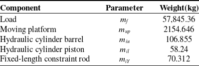
Equation (85) is derived twice to calculate the linear acceleration and angular acceleration of the moving platform. The force and moment of inertia acting on the moving platform are then determined. Using Eq. (83), the driving forces of the three driving branches are calculated in the simulation analysis software. The three-dimensional model is imported into multi-body dynamic motion analysis software for dynamic simulation. The driving force curves of the three driving branches obtained from both methods are analyzed and compared. As an example, the stable compensation of ship heave, roll, and pitch movements under Sea State 4 is used for dynamic solution verification. The mass attributes of each component of the stabilization platform are presented in Table I.

Table I.

The quality of each moving member.

Table I. Long description

The table presents the mass attributes of different components of a stabilization platform. It includes six components: Load, Moving platform, Hydraulic cylinder barrel, Hydraulic cylinder piston, and Fixed-length constraint rod. Each component is listed with its corresponding parameter and weight in kilograms. The Load has a weight of 57.845.36 kilograms, the Moving platform weighs 2154.646 kilograms, the Hydraulic cylinder barrel weighs 106.855 kilograms, the Hydraulic cylinder piston weighs 58.24 kilograms, and the Fixed-length constraint rod weighs 70.312 kilograms. The table provides a clear breakdown of the weights associated with each component, which are essential for dynamic simulation and analysis.

To verify the correctness of the theory proposed in this paper, the pose and position changes of the moving platform in three single-degree-of-freedom directions of the parallel stabilization platform are numerically set. 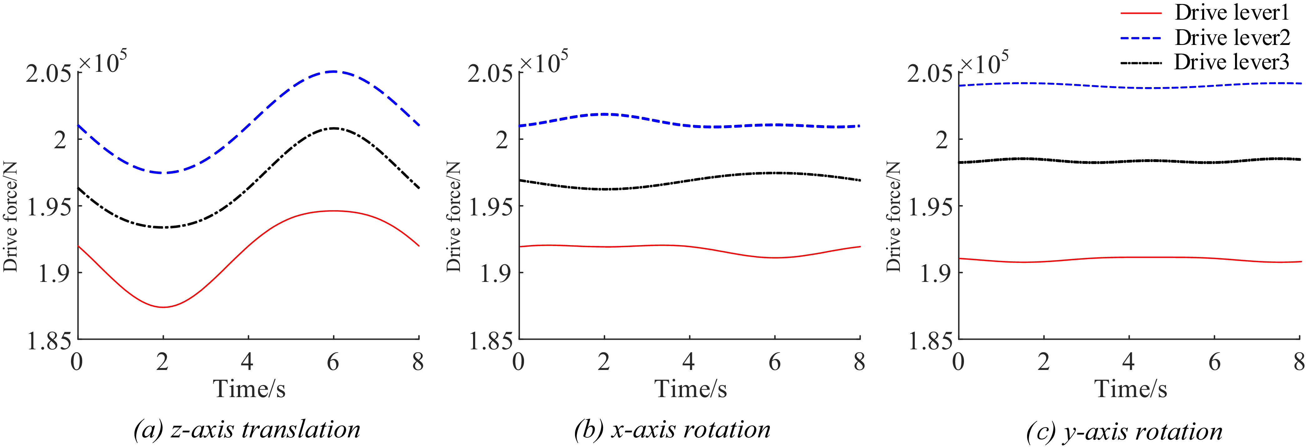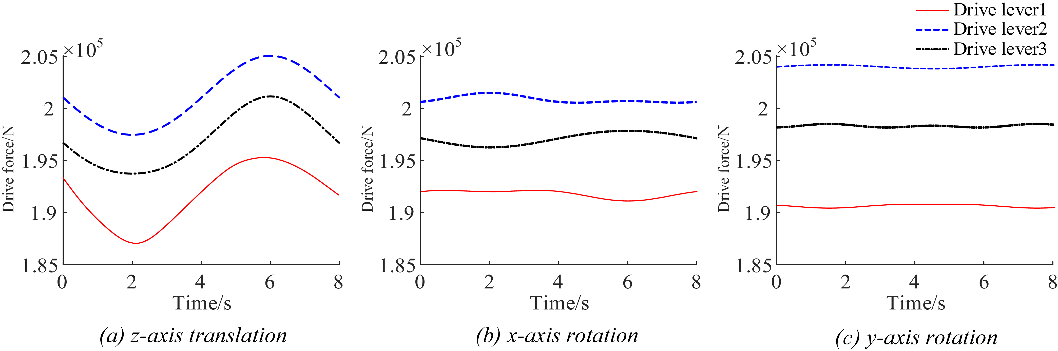The translational motion along the z-axis is defined as P _z = o _z = ±300 mm, the rotational motion angle around the x-axis is set as R _x = $\gamma$ = ±8°, and the rotational motion angle around the y-axis is set as R _y = $\beta$ = ±8°. By comparing and analyzing the driving input force change curves of the three driving rods based on the numerical simulation results from MATLAB and the simulation calculation results from ADAMS, the driving force curve charts generated by MATLAB and ADAMS are presented, as shown in Figures 6 and 7.

Figure 5.

Simplified ADAMS model of 3UPS-3SS parallel stabilization platform.

Figure 5. Long description

Figure 5 shows a simplified ADAMS model of a 3UPS-3SS parallel stabilization platform. This model features a central platform supported by three UPS (Universal-Prismatic-Spherical) joints and three SS (Spherical-Spherical) joints. The UPS joints are connected to the base with vertical prismatic joints, allowing for linear movement, while the SS joints provide rotational freedom. The structure is designed to ensure high rigidity, speed, and load capacity, making it suitable for applications in industrial manufacturing, aerospace, and ocean engineering. The model is depicted in a three-dimensional view, highlighting the geometric arrangement and mechanical connections of the components.

Figure 6.

MATLAB drive force curve of z-axis translation, x-axis rotation, and y-axis rotation.

Figure 6. Long description

The image contains three line graphs side by side. Each graph plots drive force in Newtons on the y-axis against time in seconds on the x-axis. The first graph shows the drive force curve for z-axis translation, the second for x-axis rotation, and the third for y-axis rotation. Each graph includes three lines representing different drive levers, with distinct colors and line styles for each. The drive force values range from 1.85 times 10 to the power of 5 to 2.05 times 10 to the power of 5 Newtons, and the time ranges from 0 to 8 seconds.

Figure 7.

ADAMS drive force curve of z-axis translation, x-axis rotation, and y-axis rotation.

Figure 7. Long description

The image contains three line graphs side by side. Each graph displays the drive force in Newtons on the y-axis and time in seconds on the x-axis. The first graph on the left shows the drive force curve for z-axis translation, with three different drive levers represented by red, blue, and black lines. The middle graph shows the drive force curve for x-axis rotation, again with three different drive levers. The right graph shows the drive force curve for y-axis rotation, with the same three drive levers. The red line represents drive lever 1, the blue dashed line represents drive lever 2, and the black dotted line represents drive lever 3. The graphs illustrate how the drive force varies over time for each axis and lever combination.

By comparing and analyzing the driving force curves obtained from theoretical calculations and numerical simulations, it is evident that the amplitude and trend of both are largely consistent, which preliminarily verifies the effectiveness of the established dynamic model.

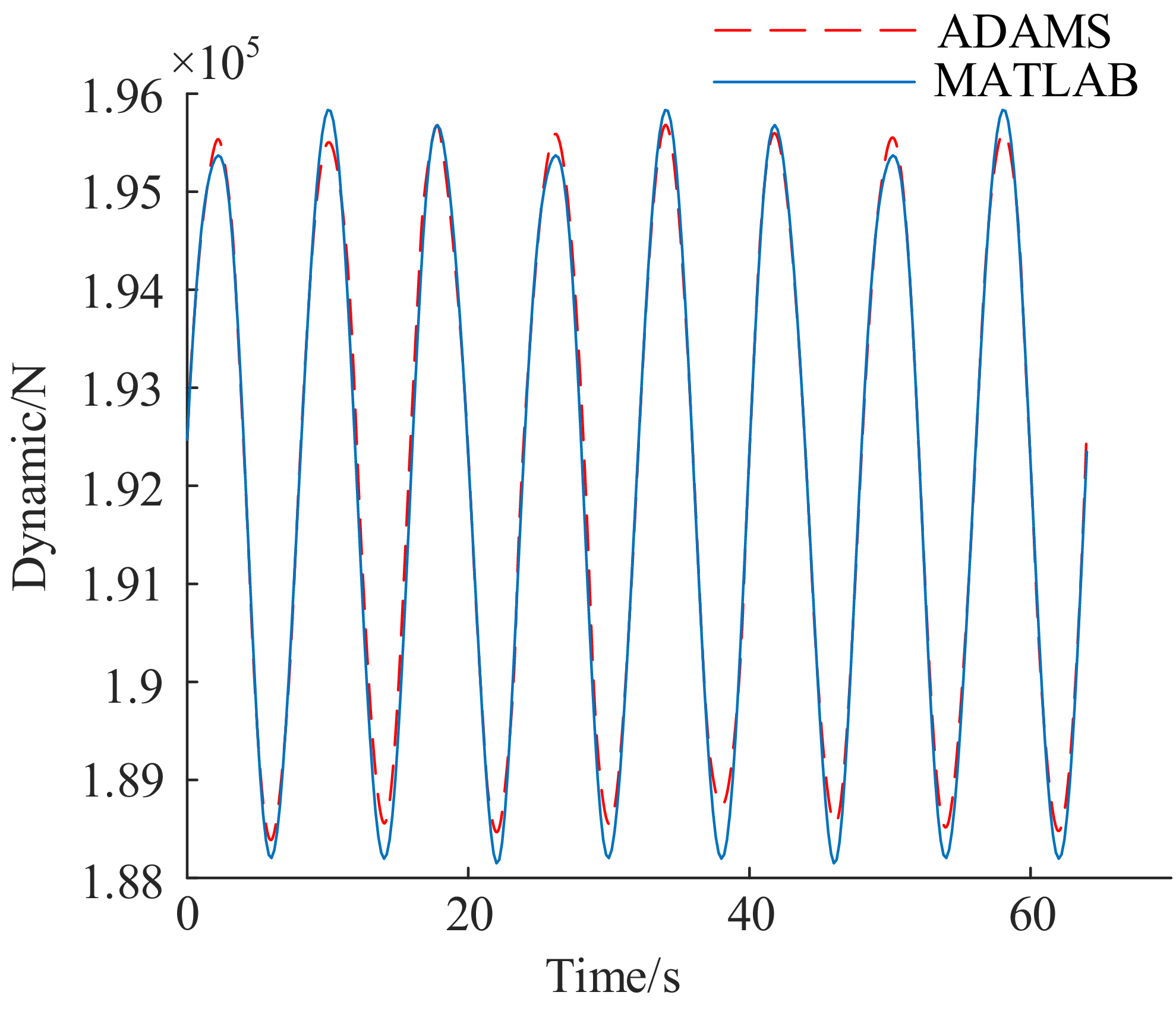
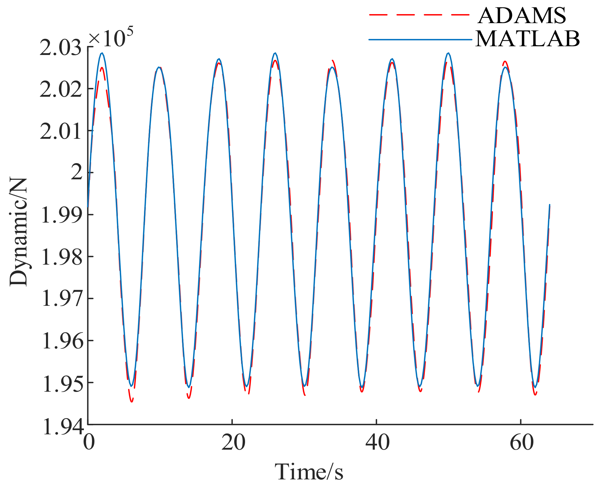
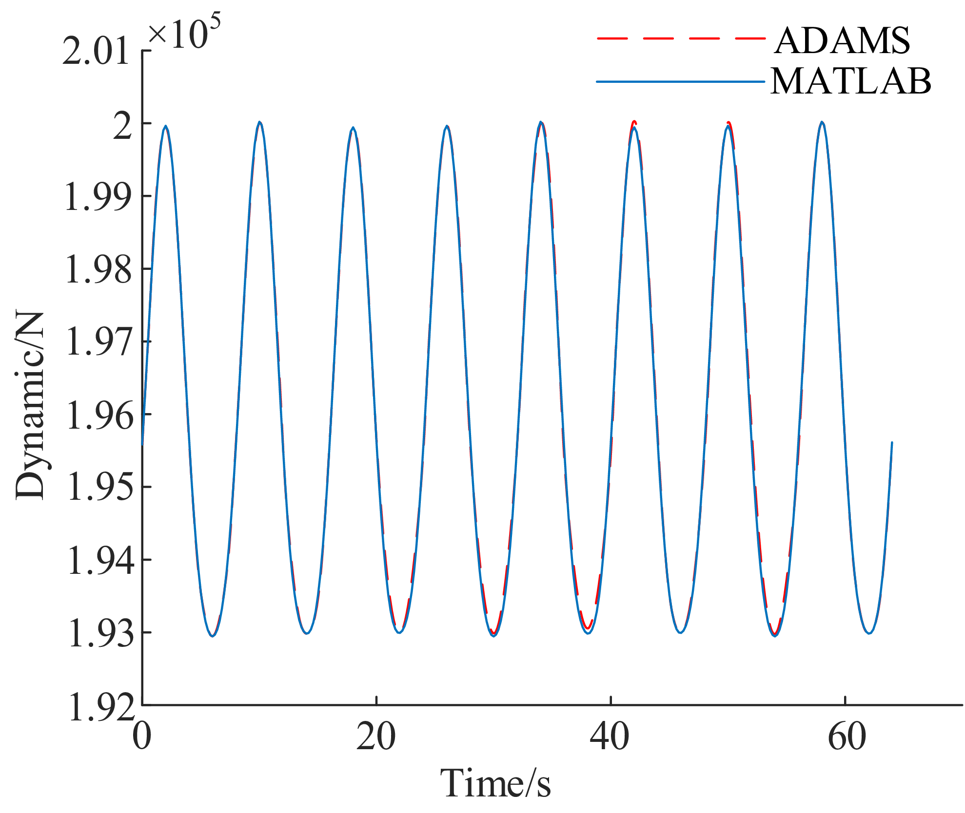
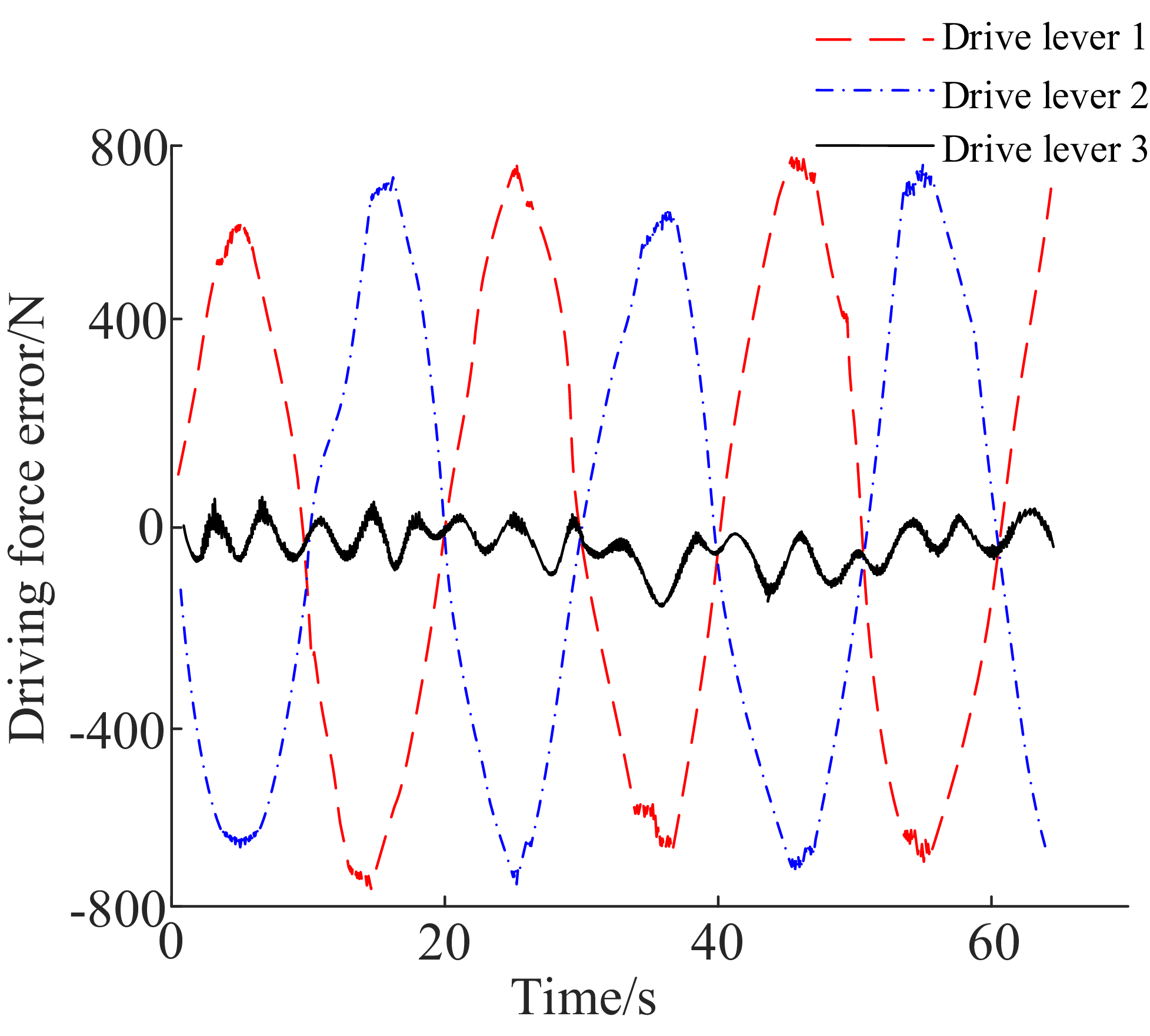
From Figures 8–10, it can be observed that the theoretical calculations based on simulation analysis software are largely consistent with the curves simulated by multi-body dynamics analysis software. The differences are illustrated in Figure 11. The maximum driving force error for drive rods 1 and 2 is 760.43 N, while the maximum driving force error for drive rod 3 is 92.86 N.

Figure 8.

Comparison curve of the simulated and theoretical driving force of the drive rod 1.

Figure 8. Long description

A line graph compares the simulated and theoretical driving force of the drive rod 1 over time. The x-axis represents time in seconds, ranging from 0 to 70 seconds. The y-axis represents the dynamic force in Newtons, ranging from 1.88 times 10 to the power of 5 to 1.96 times 10 to the power of 5. The graph features two data lines: a red dashed line representing the ADAMS simulation and a solid blue line representing the MATLAB simulation. Both lines exhibit a periodic pattern with peaks and troughs, indicating fluctuations in the driving force over time. The red dashed line closely follows the blue solid line, suggesting a strong correlation between the simulated and theoretical data. All values are approximated.

Figure 9.

Comparison curve of the simulated and theoretical driving force of the drive rod 2.

Figure 9. Long description

The line graph compares the simulated and theoretical driving force of the drive rod 2 over time. The x-axis represents time in seconds, ranging from 0 to 70 seconds. The y-axis represents the dynamic force in newtons, ranging from 1.94 times 10 to the power of 5 to 2.03 times 10 to the power of 5. Two data lines are plotted: one in red representing ADAMS and one in blue representing MATLAB. Both lines exhibit a periodic pattern with peaks and troughs, indicating fluctuations in the driving force over time. The red and blue lines closely follow each other, suggesting a strong correlation between the simulated and theoretical values. All values are approximated.

Figure 10.

Comparison curve of the simulated and theoretical driving force of the drive rod 3.

Figure 10. Long description

A line graph compares the simulated and theoretical driving force of the drive rod 3 over time. The x-axis represents time in seconds, ranging from 0 to 70 seconds. The y-axis represents the dynamic force in newtons, ranging from 1.92 times 10 to the power of 5 to 2.01 times 10 to the power of 5 newtons. The graph features two data lines: a red dashed line labeled ADAMS and a blue solid line labeled MATLAB. Both lines exhibit a periodic pattern with peaks and troughs, indicating fluctuations in the driving force over time. The values oscillate between approximately 1.93 times 10 to the power of 5 and 2.00 times 10 to the power of 5 newtons. The two lines closely follow each other, suggesting a strong correlation between the simulated and theoretical data. All values are approximated.

Figure 11.

Simulation and theoretical driving force error curves.

Figure 11. Long description

The line graph displays the driving force error over time for three drive levers. The x-axis represents time in seconds, ranging from 0 to 60 seconds. The y-axis represents the driving force error in Newtons, ranging from -800 to 800 Newtons. The graph includes three data lines: Drive lever 1 represented by a red dashed line, Drive lever 2 represented by a blue dashed line, and Drive lever 3 represented by a black solid line. Drive lever 1 and Drive lever 2 exhibit large oscillations, peaking at approximately 800 Newtons and troughing at approximately -800 Newtons. Drive lever 3 shows smaller oscillations, staying close to the zero line. All values are approximated.

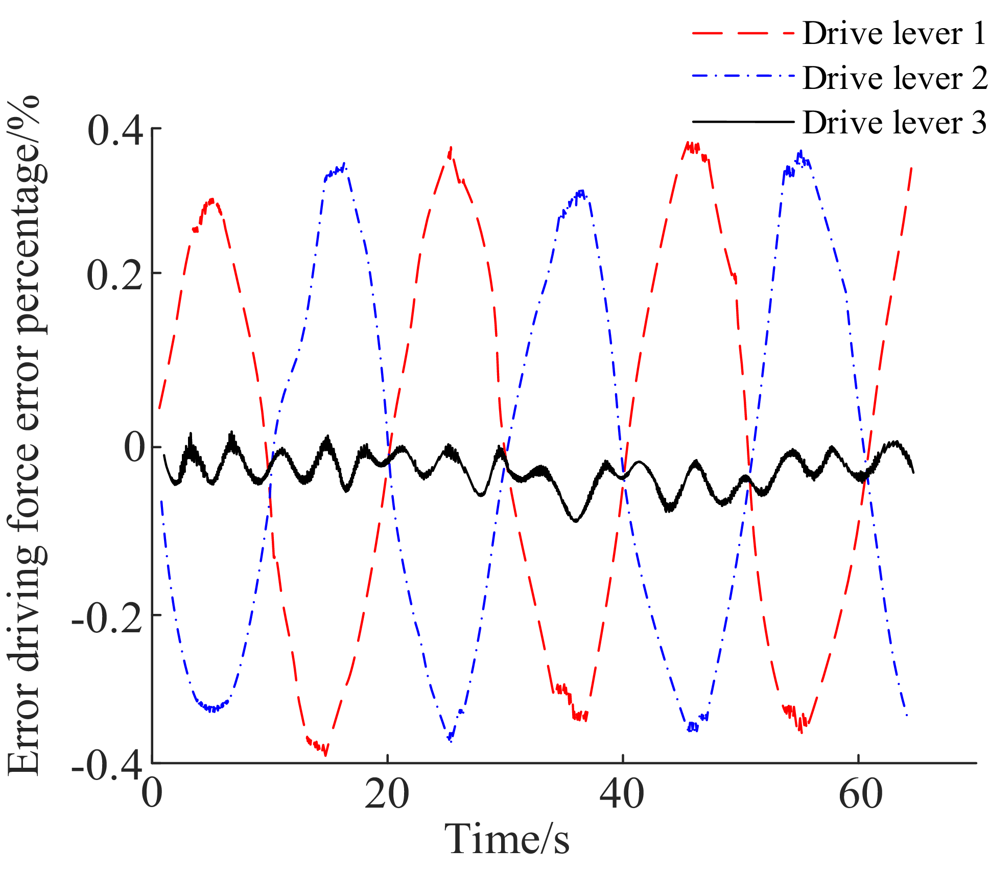
The three-dimensional geometric solid model constructed in ADAMS multi-rigid-body simulation assigns a uniform mass distribution attribute to each connecting rod. In the MATLAB simulation environment, a theoretical calculation model is built to represent all linkages using only one centroid position. When the moving platform deviates from its initial position and undergoes motion, each driving link produces rotational motion, generating additional moments of inertia. This leads to deviations between the two simulation methods. As the deviation of the moving platform from its initial position increases, the discrepancy between the methods gradually widens. Consequently, there is a certain degree of error between the driving force variation curves obtained from MATLAB and ADAMS. The peak of this error typically occurs at the peak and valley positions of the curve, which has been shown in Figure 12.

Figure 12.

Simulation and theoretical driving force error rate curves.

Figure 12. Long description

The line graph displays the error driving force error percentage over time for three drive levers. The x-axis represents time in seconds, ranging from 0 to 60 seconds. The y-axis represents the error driving force error percentage, ranging from negative 0.4 to 0.4 percentage. The graph includes three data lines: a red dashed line for Drive lever 1, a blue dashed-dotted line for Drive lever 2, and a black solid line for Drive lever 3. Drive lever 1 and Drive lever 2 exhibit periodic fluctuations with peaks and troughs, while Drive lever 3 remains relatively stable around the zero mark. All values are approximated.

Due to the inaccurate overlap between the centroid positions of the hydraulic cylinder piston, cylinder liner, and mobile platform in the ADAMS simulation model and the centroid coordinates set in MATLAB, there is a certain deviation in the driving force of the driving branch. The driving forces generated by the three driving branches were analyzed using two calculation methods. It was found that the deviation percentages did not exceed 0.4%, specifically 0.390%, 0.398%, and 0.128%, respectively. The small deviation percentages between the theoretical calculations and numerical simulation results indicate that the established dynamic simulation model is highly reliable.

6.1. Workspace analysis

The workspace is an important indicator for evaluating the kinematic performance of parallel mechanisms [Reference Zhang, Yang, Liu, Wang and Guo22, Reference Zhang, Wang, Song, Guo, Liu and Kou23]. The quick polar coordinate search steps for setting up a workspace start from the initial angle. The polar diameter increases in increments of 0 mm. When the length of the telescopic rod l and the rotation angle of the pair reach their limit values, the endpoint of the polar diameter becomes the boundary point of the workspace. The domestic nearshore waters primarily experience Sea State 4. The structural parameters selected for stable compensation of ship heave, roll, and pitch movements [Reference Hongbin, Song, Feng, Xue and Lijie4] under this sea condition are shown in Table II.

Table II.

Stabilize the structural parameters of the platform.

Table II. Long description

The table presents structural parameters for stabilizing a platform, including fixed-platform circumference radius, moving platform circumference radius, length of constraint rod, horizontal distance between specific points, drive dead zone, drive travel, limit values for Hooke joint angle and ball pair rotation angle, vertical distance between a point and the moving platform, and initial height difference between moving and stationary platforms. The table contains two columns: Parameter and Numerical value, with 10 rows detailing specific measurements in millimeters and degrees.

Set the constraints for the workspace as follows:

(102) \begin{align} \begin{cases} l_{\min }=l_{d}+l_{s}\\[5pt] l_{\max }=l_{d}+l_{s}+l_{s}\\[5pt] \theta _{ai}=\theta _{a\max }\\[5pt] \theta _{bj}=\theta _{b\max } \end{cases} \end{align}

where l _max, l _min represent the maximum and minimum lengths of the driving rod, respectively. $\theta$ _ai is the size of the Hooke joint angle; $\theta$ _bj ( j = 1, 2, …, 9) is the size of the ball pair angle

Figure 13.

Institutions have access to workspaces.

Figure 13. Long description

The image contains four subplots of a scatter plot. Each subplot presents a different view of a grid with color gradients ranging from blue to yellow. The front view (a) and left view (b) show the grid in a 3D space with the z-axis labeled in millimeters and the x-axis labeled in degrees. The vertical view (c) displays the grid in a 2D plane with both axes labeled in degrees. The 3D view (d) combines all three dimensions, showing the grid in a three-dimensional space with axes labeled in degrees and millimeters. The grid appears to form a conical shape in the 3D views and a circular shape in the vertical view. The color gradients indicate variations in the data points across the grid. All values are approximated.

Use Matlab software to draw the workspace using the fast polar coordinate method as shown in Figure 13. As shown in the figure, the workspace of this mechanism is relatively large and not of a regular shape, so its volume cannot be explicitly expressed. This article uses the bounding box method [Reference Kim, Lee, Kim and Han24] to enclose the workspace into a regular shape and calculate its volume V _W , as follows:

(103) \begin{equation} V_{W}=\left(x_{\max }-x_{\min }\right){\boldsymbol\cdot} \left(y_{\max }-y_{\min }\right){\boldsymbol\cdot} \left(z_{\max }-z_{\min }\right) \end{equation}

where x _max, y _max, and z _max represent the maximum coordinate values of the workspace in the x, y, and z directions. x _min, y _min, and z _min represent the minimum coordinate values of the workspace in the x, y, and z directions.

6.2. Force transmission analysis

The force Jacobian matrix describes the relationship between the force acting on the driving rod and the force acting on the moving platform, as follows:

(104) \begin{equation} {\boldsymbol{F}}_{F}={\boldsymbol{H}}{\boldsymbol\cdot} \boldsymbol{\tau }_{j} \end{equation}

where F _F is the force and torque experienced by the moving platform. $\boldsymbol\tau_{j}$ is the driving force of the driving rod. H is the Jacobian matrix of forces.

In the field of mechanics, if the force Jacobian matrix H is the transpose J ^T of the velocity Jacobian matrix J , then Eq. (38) can be transformed into:

(105) \begin{equation} \boldsymbol{\tau }_{j}={\boldsymbol{H}}^{-1}{\boldsymbol\cdot} {\boldsymbol{F}}_{F}=\left({\boldsymbol{J}}^{\mathrm{T}}\right)^{-1}{\boldsymbol\cdot} {\boldsymbol{F}}_{F} \end{equation}

By performing singular value decomposition on the velocity Jacobian matrix J in Eq. (39), the range of values for the driving force $\boldsymbol\tau_{j}$ of the driving rod can be obtained as follows:

(106) \begin{equation} \frac{\left|\left|{\boldsymbol{F}}_{F}\right|\right|}{\sigma _{\max }\left({\boldsymbol{J}}\right)}\leq \left|\left|\boldsymbol{\tau }_{j}\right|\right|\leq \frac{\left|\left|{\boldsymbol{F}}_{F}\right|\right|}{\sigma _{\min }\left({\boldsymbol{J}}\right)} \end{equation}

The upper limit of the driving force of the driving rod is determined by the minimum singular value $\sigma$ _min( J ) of the velocity Jacobian matrix J . When $\sigma$ _min( J ) decreases, the upper limit increases, the mechanism approaches a singular pose, and the force transmission efficiency decreases. On the contrary, as the upper limit decreases, the mechanism approaches isotropy, and the force transmission performance improves. Therefore, $\sigma$ _min( J ) can be used as a local force transfer performance index (LTI).

LTI only reflects the force transmission performance of the mechanism in a specific pose and cannot evaluate the overall force transmission performance of the mechanism. To compensate for the shortcomings of LTI indicators, the Global Force Transfer Index (GTI) is introduced. Starting from the definition of transmission angle, the area with a local force transmission performance index greater than 0.7 in the workspace is defined as a high-quality transmission space. The ratio of high-quality transfer space to the overall workspace is the GTI, which is expressed as:

(107) \begin{equation} \psi_{\mathrm{GTI}}= \frac{\int\limits_{V_{G}} \mathrm{d}W} {\int\limits_{V_{W}} \mathrm{d}W} \end{equation}

where W is the overall workspace of the institution, V _G is the volume of the high-quality transmission space, and V _W is the volume of the overall workspace.

The value of $\psi$ _GTI ranges from 0 to 1, and the closer it is to 1, the better the force transmission performance of the mechanism. The closer it approaches 0, the closer the mechanism approaches a singular state, and the transmission efficiency of force from the driving end to the end effector decreases.

Based on the above definition and the parameters in Section 3.1, search for the distribution map of the minimum singular value of the Jacobian matrix, as shown in Figure 14. As shown in the figure, the $\sigma$ _min( J ) of the mechanism in the majority of the target workspace is greater than 0.3, with an average minimum singular value of $\overline{\mathit{\sigma }}_{\min }({\boldsymbol{J}})$ of 0.28, corresponding to $\psi$ _GTI of 0.46. This indicates that the overall force transmission performance of the mechanism is poor, especially in the boundary region of the workspace where $\sigma$ _min( J ) is between 0 and 0.1, which is close to a singular pose.

Figure 14.

Minimum singular value distribution.

Figure 14. Long description

A scatter plot visualizes the distribution of minimum singular values in a parallel mechanism. The plot contains hundreds of data points, each represented by a colored dot. The x-axis represents the beta angle in radians, ranging from negative ten to positive ten radians. The y-axis represents the z-axis position in millimeters, ranging from negative one hundred to positive one hundred millimeters. The color gradient from blue to yellow indicates the magnitude of the singular values, with blue representing lower values and yellow representing higher values. The data points form a cluster that appears to have a central concentration with a spread towards the outer regions. The overall trend suggests a variation in singular values across different configurations of the mechanism. All values are approximated.

6.3. Dynamic dexterity analysis

The 3UPS-3SS mechanism is a 2R1T low-degree-of-freedom parallel mechanism with an inherently asymmetric structure. The drive branch chain adopts a UPS configuration, while the constraint branch chain adopts an SS configuration. The motion constraint characteristics of these two configurations differ significantly, resulting in a mass matrix that cannot achieve ``completely equal singular values in all directions,’’ which is the core condition for ideal isotropy. Additionally, the motion space of the mechanism is limited to translation along the z-axis and rotation around the x/y axes. It lacks the freedom of rotation around the z-axis and translation along the x/y axes. As a result, the ``isotropy’’ of the dynamic response is inherently dimensionally restricted, making the pursuit of ideal isotropy for the entire space impractical.

Dynamic isotropy represents an extreme case of ``optimal dynamic dexterity,’’ but there is a strong coupling conflict between this goal and the workspace and force transmission performance [Reference Singh, Ahmad and Ghosal5]. Excessively pursuing isotropy leads to a deviation of the mechanism’s scale parameters toward ``symmetry and compactness,’’ sacrificing workspace and force transmission efficiency. This paper emphasizes practical configurations that balance multiple objectives rather than theoretical configurations optimized for a single index. Therefore, it does not focus solely on the extreme case of dynamic isotropy.

During the process of cargo transshipment at sea, changes in the weight and shape of the cargo demand good load adaptability. High dynamic agility optimizes load distribution for the system. This optimization allows the system to handle goods of different weights and shapes effectively. It also helps avoid instability or reduced accuracy caused by uneven loads.

In order to ensure a uniform distribution of acceleration in all directions of the mechanism, thereby enhancing its dynamic isotropy and improving overall dynamic agility, the condition number of the mass matrix is usually used for evaluation. The condition number ( M = J ^T I ( q ) J ) of the mass matrix is calculated and used to measure local dynamic dexterity (LDD). The specific calculation equation is as follows:

(108) \begin{align} \quad \quad K_{M}&=\left|\left|{\boldsymbol{M}}\right|\right|{\boldsymbol\cdot} \left|\left|{\boldsymbol{M}}^{-1}\right|\right| \nonumber \\[5pt] &=\dfrac{\sigma _{\max }\left({\boldsymbol{M}}\right)}{\sigma _{\min }\left({\boldsymbol{M}}\right)} \nonumber \\[5pt] &=\sqrt{\lambda _{\max }\left({\boldsymbol{M}}^{{\boldsymbol{T}}}{\boldsymbol{M}}\right)}{\boldsymbol\cdot} \sqrt{\lambda _{\max }\left({\boldsymbol{M}}^{-\mathrm{T}}{\boldsymbol{M}}^{-1}\right)} \end{align}

(109) \begin{equation} \begin{aligned} K_{{\boldsymbol{M}}}&=\left|\left|{\boldsymbol{M}}\right|\right|{\boldsymbol\cdot} \left|\left|{\boldsymbol{M}}^{-1}\right|\right|\\[5pt] &=tr\left({\boldsymbol{M}}^{\mathrm{T}}{\boldsymbol{M}}\right)^{1/2}{\boldsymbol\cdot} tr\left({\boldsymbol{M}}^{-\mathrm{T}}{\boldsymbol{M}}^{-1}\right)^{1/2} \end{aligned} \end{equation}

where K _M is the condition number of the mass matrix, and after normalization, its value ranges from 0 to 1. The closer it approaches 1, the worse the acceleration performance of the mechanism. The closer it approaches 0, the better the acceleration performance of the mechanism.

The dynamic dexterity of a mechanism is influenced by its geometric structural parameters and exhibits a trend of variation throughout the entire workspace. In order to measure the overall dynamic performance of the mechanism, the Global Dynamic Dexterity Index (GDD) $ \eta$ _M is commonly used, which characterizes the comprehensive dynamic sensitivity of the mechanism by calculating the average local dynamic dexterity of the entire workspace.

(110) \begin{equation} \eta _{M}=\frac{\int \limits_{W}K_{M}dW}{\int \limits_{W}dW} \end{equation}

Based on the above definition and parameters in Section 2.2, the distribution map of the local dynamic dexterity of the mechanism shown in Figure 15 is obtained through searching. By analyzing the corresponding data through the diagram, it can be concluded that within the workspace of the mechanism, the condition number K _M of the mass matrix in most areas exceeds 0.4, while the global dynamic dexterity index $ \eta$ _M is 0.79. This indicates that the overall acceleration transfer performance of the mechanism is weak, especially in the workspace boundary area K _M between 0.9 and 1, which is close to anisotropy, and the mechanism needs further optimization.

Figure 15.

Institutional LDD distribution map.

Figure 15. Long description

A 3D heat map with axes labeled beta and gamma in degrees and z in millimeters. The map displays a color gradient ranging from blue to yellow, indicating varying values. The highest values are represented by yellow, while the lowest values are shown in blue. The heat map features a central peak with higher values and gradually decreases towards the edges. The color scale on the right side of the image ranges from 0 to 1, providing a visual representation of the data distribution.

7.1. Establish an optimization model

The overall performance of the institution is influenced by its scale parameters. In the scale optimization problem, the scale parameters include length variables and mass variables. The decision variables for this optimization design problem are defined as follows:

(111) \begin{equation} \begin{aligned} {\boldsymbol{x}}&=\left(x_{1},x_{2},\ldots ,x_{D}\right)^{\mathrm{T}}\\[5pt] & =\left(R_{a},R_{b},h_{1},l_{m},l_{n},l_{d},l_{s},m_{iu},m_{il},m_{iY}\right)^{\mathrm{T}} \end{aligned} \end{equation}

Where D is the dimension of the decision variable.

To improve the overall force transmission performance of the mechanism in the workspace and achieve high force transmission efficiency in as many areas as possible, the optimization objective is to maximize the average minimum singular value f ₂(x). In the process of optimizing mechanism design, increasing the workspace may lead to weaker force transmission ability in certain positions of the mechanism, as the increase in space may result in the arrangement of pairs and components no longer being dominant, thereby affecting the transmission efficiency. Meanwhile, expanding the workspace may lead to a decrease in the stiffness and dynamic performance of the mechanism, especially during dynamic response and control, which may result in a decrease in dexterity. Therefore, maximizing the workspace volume f ₁(x), minimizing the condition number f ₃(x) of the average mass matrix of the mechanism, and maximizing the average minimum singular value f ₂(x) of the mechanism are a set of contradictory objectives that can be used as three objectives in scale parameter optimization. The objective function of this optimization problem can be set to:

(112) \begin{align} \min \begin{cases} f_{1}(x)=1/V_{W}\\[5pt] f_{2}(x)=1/\overline{\sigma }_{\min }\left(J\right)\\[5pt] f_{3}(x)=\eta _{M} \end{cases} \end{align}

To ensure that the mechanism can adapt to the range of ship motion, avoid interference, prevent mechanism singularity, and optimize force transmission performance, the following constraints are introduced:

1) Limitations on decision variable values. To ensure adaptability to the range of ship motion, the decision variable values are confined within a specific range, as shown in Table III:

Table III.

The range of values of the decision variables.

Table III. Long description

The table presents the upper and lower limits of decision variables, including dimensions in millimeters and mass in kilograms. It contains eight rows and two columns, with the first column listing variables such as R subscript o, R subscript b, h subscript 1, l subscript m, l subscript b, l subscript d, m subscript 10, and m subscript 0. The second column shows the corresponding upper and lower limits for each variable. For instance, R subscript o and R subscript b both range from 650 to 1950 millimeters, while h subscript 1 ranges from 136 to 406 millimeters. Mass variables like m subscript 10 and m subscript 0 have limits ranging from 29.12 to 160.28 kilograms and 35.16 to 105.48 kilograms, respectively.

2) Mass constraints. In optimizing quality parameters, it is assumed that the rotational inertia of each component remains constant. This assumption simplifies calculations and enhances optimization efficiency. Only the influence of component mass on the dynamic characteristics of the mechanism is analyzed. Additionally, the quality of the dynamic platform is determined by external load changes to ensure rationality in optimization calculations. Therefore, the dynamic platform and load mass are set at a constant value of 60,000 kg. The minimum sum of the masses of other moving parts, calculated based on the original mass of each component, is as follows:

(113) \begin{equation} m_{\min }=\mathop{\sum }\limits_{i=1}^{3}\left(m_{iu,\min }+m_{il,\min }+m_{iY,\min }\right)=706.221\,\mathrm{kg} \end{equation}

The design variables in the optimization process should meet the overall constraints:

(114) \begin{equation} \mathop{\sum }\limits_{i=1}^{3}\left(m_{iu}+m_{il}+m_{iY}\right)\gt m_{\min } \end{equation}

3) Hook pair and ball pair angle limit: To prevent interference, the rotation angles of the Hooke pair and ball pair are limited within a defined range:

(115) \begin{align} \begin{cases} g_{j}(x)=\theta _{bj}-\theta _{b\max }\leq 0\\[5pt] g_{i+9}(x)=\theta _{ai}-\theta _{a\max }\leq 0 \end{cases} \end{align}

4) Avoiding singular configurations. To ensure optimal transmission performance of the mechanism, the following constraint conditions are introduced:

(116) \begin{equation} g_{13}(x)=\sigma _{\min ,\min }=\min \sigma _{\min }\left({\boldsymbol{J}}\right)\geq 0.2 \end{equation}

where $\sigma$ _min,min is the minimum value among the minimum singular values in the workspace.

7.2. NSGA-III multi-objective optimization method

The optimization of parallel mechanism scale parameters is a multi-objective optimization problem. The NSGA-III algorithm was proposed by DEB et al. [Reference Deb and Jain25] as a method for solving such problems. Its working principle is illustrated in Figure 16. The NSGA-III algorithm removes the crowding distance selection used in NSGA-II and introduces reference points. This change reduces computational costs and improves the convergence of the algorithm. It also increases the diversity of solutions and accelerates the search process. The method is suitable for high-dimensional multi-objective problems with three or more objectives. The flowchart of the NSGA-III algorithm is shown in Figure 17.

Figure 16.

Schematic diagram of the NSGA-III algorithm.

Figure 16. Long description

The flowchart illustrates the NSGA-III algorithm process. It begins with a population Pt and a set of reference points Rt. The population is divided into different fronts F1 to Fn based on non-dominated sorting. Each front is then mapped to the reference points. The process includes a step labeled ’Small habitat protection’ which filters the population. The final population Pt+1 is formed, with some individuals being marked as ’Give up’. The flowchart shows the flow of individuals through these stages, indicating the selection and sorting mechanism of the algorithm.

Figure 17.

NSGA-III algorithm flowchart.

Figure 17. Long description

The flowchart illustrates the NSGA-III algorithm process. It begins with initialization, followed by generating the initial parent generation. The process then involves crossing and mutation to generate offspring, merging parent and child populations, and performing non-dominated sorting. The population selection strategy includes establishing reference points on the hyperplane, population normalization, calculating the vertical distance of the population, and small habitat protection operations. This strategy generates the next generation of the parent population. The process repeats until the requirements are met, at which point the optimal population is outputted.

The NSGA-III algorithm includes the following basic steps:

Step 1: Set parameters such as iteration count, population size, mutation probability, crossover probability, etc., and initialize the reference point and population.

Step 2: Perform selection, crossover, and mutation operations on the parent population P_t to obtain the offspring Q_t , and calculate the fitness of all individuals in Q_t separately.

Step 3: Merge the parent and offspring populations to obtain a new population R_t and divide it into different levels of non-dominated fronts through non-dominated sorting, such as F ₁, F ₂, …, F _l , …, F _n .

Step 4: Starting from the non-dominated layer of F ₁, select individuals in sequence and keep them in the next generation population S_t until the number of individuals in S_t is greater than or equal to the population size N. If the selected individual is in the F _l layer at this time, discard the remaining individuals in the non-dominated layer after F _l . If the number of individuals in S_t is equal to n at this time, the iteration ends, and S_t is used as the parent population P _{t + 1} for the next iteration. If the number of individuals in S_t is greater than n at this time, all individuals before the non dominated layer F _l will be stored in the next iteration’s parent population P _{t + 1}, and then a population selection strategy based on the reference point will be used, that is, allocation will be based on the shortest distance. Select some individuals from F _l and store them in P _{t + 1} until the population size of P _{t + 1} reaches N, and end this iteration at the same time.

Step 5: Determine if the set number of iterations has been reached. If so, terminate the iteration and output the optimal population. Otherwise, return to step 2.

7.3. Multi-objective optimization and result analysis

The NSGA-III algorithm uses a population size of 200. The crossover probability is set to 0.5, and the mutation probability is also set to 0.5. The iteration count is fixed at 80. The search produces 200 Pareto optimal solutions, as shown in Figure 18.

Figure 18.

Pareto optimal solution set.

Figure 18. Long description

A 3D scatter plot with red dots representing data points, showing the relationship between three variables labeled as f1(x), f2(x), and f3(x). The x-axis represents f1(x) ranging from 0.75 to 1.6, the y-axis represents f2(x) ranging from 0.8 to 1, and the z-axis represents f3(x) ranging from 0.2 to 0.7. The data points are scattered throughout the 3D space, forming a cloud-like distribution. There is no clear linear trend visible, and the points are densely packed in the center, becoming sparser towards the edges. The plot appears to illustrate the inertial forces acting on various moving components within a stabilization platform, following the D’Alembert principle. All values are approximated.

This article focuses on three objective optimizations. It uses the TOPSIS method [Reference Pandey, Komal and Dincer26] to rank evaluation objects based on their proximity to the ideal objective. The method helps determine how each objective impacts overall performance. The calculation method for its evaluation indicators is outlined below:

(117) \begin{equation} C=\frac{D^{-}}{D^{-}+D^{+}} \end{equation}

Where D ⁺ is the distance from the solution to the optimal solution. D ⁻ is the distance to the worst solution.

The comparison between several representative solutions selected from the Pareto solutions obtained and the original design parameters is shown in Table IV.

Table IV.

Comparison of mechanism performance parameters before and after optimization.

Table IV. Long description

The table presents a comparison of mechanism performance parameters before and after optimization across five groups. It includes measurements for Ra, Rb, h1, lm, ln, ls, ld, miu, mil, miY, f1(x), f2(x), and f3(x) in various units. Each group shows variations in these parameters, indicating changes due to optimization. For example, Group 1 shows an increase in Ra from 1.300 meters to 1.456 meters after optimization, while Group 5 shows a significant increase in miY from 70.31 kilograms to 93.44 kilograms.

Table V.

Comparison of mechanism performance parameters before and after optimization.

Table V. Long description

The table presents a comparison of mechanism performance parameters before and after optimization, focusing on five groups and several metrics. It includes data on volume change of workspace in percentage, change of mean minimum singular value in percentage, and dynamic dexterity variation in percentage. The table has five rows labeled Group 1 to Group 5 and three columns labeled Volume change of workspace (%), Change of mean minimum singular value (%), and Dynamic dexterity variation (%). Notable trends include significant variations in the change of mean minimum singular value and dynamic dexterity variation across different groups. For instance, Group 1 shows a volume change of workspace of plus 14.28 percentage, a change of mean minimum singular value of plus 171.43 percentage, and a dynamic dexterity variation of plus 13.92 percentage. Group 5, on the other hand, shows a volume change of workspace of minus 17.24 percentage, a change of mean minimum singular value of plus 82.14 percentage, and a dynamic dexterity variation of plus 32.91 percentage.

Figure 19.

Optimized distribution of LTI.

Figure 19. Long description

A heat map displays the optimized distribution of LTI. The map is a three-dimensional plot with axes labeled beta and gamma in degrees and z in millimeters. The color scale ranges from blue to yellow, indicating varying intensities. The highest intensity is represented by yellow, while the lowest is represented by blue. The heat map shows a gradient distribution with higher values concentrated in the center and lower values towards the edges. The plot is set within a grid layout, and the data points are densely packed, forming a smooth surface.

Excessive pursuit of a large workspace will increase the physical volume of the mechanism, which is unfavorable for installation on the ship. It can be seen from the selected optimization results from Table 5 that the average minimum singular value and dynamic dexterity of the second set of results are greatly improved, although the workspace volume is only increased by 7.14%. The corresponding mechanism scale parameters are {R _a , R _b , h ₁ , l _m , l _n , l _s , l _d , m _iu , m _il , m _iY } = {1309, 1249, 265, 1286, 319, 362, 473, 110.28, 71.28, 68.96}.

Based on the above parameters, the distribution of the minimum singular value of the optimized Jacobian matrix and the distribution of the condition number of the mass matrix are shown in Figures 19 and 20, respectively. As shown in the figure, the $\sigma$ _min( J ) of the mechanism in the target workspace is greater than 0.6, and the average minimum singular value $\overline{\mathit{\sigma }}_{\min }({\boldsymbol{J}})$ is 0.83, corresponding to a $\psi$ _GTI of 1, indicating that the overall force transmission performance of the mechanism is good. The K _M of the mechanism in the target workspace is less than 0.5, and the global dynamic dexterity index $ \eta$ _M is 0.35, indicating that the overall acceleration performance of the mechanism is good.

The comparison of performance parameters before and after institutional optimization is shown in Table VI.