Introduction

Snow cover on sea ice modulates ice/atmosphere heat exchanges due to its high albedo (Reference Grenfell and MaykutGrenfell and Maykut, 1977) and insulating properties (Reference Sturm, Holmgren, König and MorrisSturm and others, 1997, Reference Sturm, Morris, Massom and Jeffries1998, Reference Sturm, Holmgren and Perovich2001). The thermal conductivity of snow is much less than that of the underlying ice and an order of magnitude less than that of the ocean (Reference Maykut and UntersteinerMaykut and Untersteiner, 1971), which allows it to insulate the sea ice from cold polar air. The insulation decreases the basal sea-ice accumulation rate, and the high albedo impedes sea-ice melt from the top during the summer (Reference WarrenWarren and others, 1999). The summer melting of snow cover creates surface ponds, whose lower albedo absorbs more radiation than snow or ice, further increasing the rate of melt at the top and introducing a supply of fresh water into the ocean. Remote sensing of the snow depth in the polar regions provides an improved understanding of sea-ice mass balance, surface heat and energy budget, inter-annual variability of precipitation/accumulation rates and, in turn, freshwater input (Reference FarrellFarrell and others, 2012).

Satellite-based laser and radar altimeters optimized for polar observations have been launched over the last decade (Reference ZwallyZwally and others, 2002; Reference WinghamWingham and others, 2006), with the determination of global sea-ice thickness/distribution being one of the major objectives of these missions. The altimeters measure the sea-ice freeboard, which is converted to sea-ice thickness under the assumption of hydrostatic equilibrium. Sea-ice thickness is related to total freeboard and snow thickness (Reference Kwok and CunninghamKwok and Cunningham, 2008) as

where ρ _w, ρ _i and ρ _s are the densities of sea water, sea ice and snow, respectively, and h _i, h _f and h _s are sea-ice thickness, total freeboard and snow thickness, respectively. Each of the components of Eqn (1) is shown in Figure 1 as an illustration of how sea-ice thickness is calculated. Given Eqn (1), the determination of sea-ice thickness is based on freeboard (snow and ice above sea level) measurements, and the presence of snow cover affects this thickness estimate. Satellite and airborne laser altimeters, including ICESat-I (Ice, Cloud, and land Elevation Satellite-I), measure range to the air/snow interface and rely upon detection of open water (leads) to establish mean sea level. Accurate knowledge of the snow depth is necessary to back out the effect of the snow loading in the freeboard measurements. Reference Zwally, Yi, Kwok and ZhaoZwally and others (2008) used the AMSR-E (Advanced Microwave Scanning Radiometer for Earth Observing System) snow thickness product (Reference Comiso, Cavalieri and MarkusComiso and others, 2003), which is restricted to dry snow thickness of <50 cm, to estimate sea-ice thickness from ICESat-I measurements in the Weddell Sea, Antarctica. Reference Kwok and CunninghamKwok and Cunningham (2008) used the European Centre for Medium-Range Weather Forecasts (ECMWF) daily snow precipitation products to estimate sea-ice thickness from ICESat-I measurements in the Arctic Ocean. Regardless of the snow thickness product, those authors stated that the uncertainty in the snow depth leads to a large uncertainty in the sea-ice thickness estimate, which highlights the need for more accurate knowledge of snow thickness and its distribution.

Fig. 1.

Illustration of the mathematical components of sea-ice thickness measurement.

Measurements of freeboard made by satellite-based radar altimeters, which typically operate at Ku-band frequencies, are also affected by the presence of snow. For measurements collected over the Arctic sea ice during October–March, in which the snow cover is dry and cold, the peak radar return is assumed to come from the snow/ice interface (Reference Laxon, Peacock and SmithLaxon and others, 2003). This was confirmed through a comparison of data retrieved from laser and radar altimeters operating from an airborne platform (Reference GilesGiles and others, 2007; Reference LeuschenLeuschen and others, 2008). Consequently, during these months accurate sea-ice thickness estimates made from satellite radar-altimeter measurements over the Arctic contain less uncertainty due to snow loading. The origin of the peak radar return within the snow/sea-ice stratigraphy is ambiguous for the Antarctic sea-ice snow cover due primarily to the overall increased snow depth resulting from higher temperatures compared to the Arctic and the subsequent presence of an intermediate slush layer (Reference Willatt, Giles, Laxon, Stone-Drake and WorbyWillatt and others, 2010). This introduces more uncertainty into the determination of sea-ice thickness.

To improve the accuracy of sea-ice thickness estimates, an airborne radar with fine resolution for mapping snow stratigraphy and characterizing radar backscatter is needed to validate satellite-based sensors. Measurement design goals are to measure snow depth over a 0.1–2 m range with a vertical range resolution on the order of 5 cm. This vertical range resolution corresponds to an altimetric ice thickness error of 18 cm for ρ _w = 1.025 g cm⁻³, ρ _s = 0.3 g cm⁻³ and ρ _i = 0.836 g cm⁻³ (Reference Ulaby, Moore and FungUlaby and others, 1986a; Reference Kwok and CunninghamKwok and Cunningham, 2008). Towards this end, the Center for Remote Sensing of Ice Sheets (CReSIS) at the University of Kansas has developed a 2–8 GHz ultra-wideband (UWB), frequency-modulated, continuous-wave (FMCW) radar capable of detecting snow thickness over sea ice. The lower frequency range was selected because of the reduced attenuation in snow, but is still high enough to provide the large bandwidth necessary to achieve the targeted range resolution. This radar has been successfully operated on long-range NASA aircraft since 2009.

The application of UWB radars for measuring snow depth has been the topic of several investigations starting in the 1970s (Reference Venier and CrossVenier and Cross, 1972; Reference Vickers and RoseVickers and Rose, 1973; Reference Koh, Yankielun and BaptistaKoh and others, 1996; Reference Holmgren, Sturm, Yankielun and KohHolmgren and others, 1998; Reference KanagaratnamKanagaratnam and others, 2007; Reference Marshall and KohMarshall and Koh, 2008; Reference Marshall, Birkeland, Elder, Meiners, Campbell, Conger and HaegeliMarshall and others, 2008). Most of these measurements were performed either with surface- or helicopter-based radars. The results from the surface-based measurements demonstrated the potential of UWB radars for snow depth determination. However, the airborne experiments were of limited success because the technology required to implement high-sensitivity, UWB, coherent radars was not available at the time these systems were developed. Most of the earlier airborne systems used Yttrium iron garnet (YIG)-tuned oscillators to generate a UWB chirp. YIG oscillators are limited to sweep rates in the millisecond range and cannot be swept at the fast rate (μs) required for airborne applications. Recent advances in microwave and digital device technologies enabled the development of UWB chirp generators required to implement airborne systems (Reference Straayer, Messier and LyonsStrayer and others, 2006; Reference Panzer, Leuschen, Patel, Markus and GogineniPanzer and others, 2010; Reference Gomez-GarciaGomez-Garcia, 2011).

The radar described in this paper, currently known as the ‘Snow Radar’, is a much-improved version of previous systems built at CReSIS. The early version of the radar was operated over a frequency range of 2–8 GHz with a 10 ms sweep rate for surface-based measurements as part of the Australian AMSR-E sea-ice validation experiments in 2003 in the Antarctic (Reference KanagaratnamKanagaratnam and others, 2007). A modified version of the surface-based radar used a YIG oscillator for chirp generation, an improved data acquisition system and an antenna array for helicopter-based measurements of Antarctic sea-ice snow cover in 2008 with partial success (Reference Galin, Worby, Markus, Leuschen and GogineniGalin and others, 2012).

The radar system originally developed for surface-based measurements was redesigned, modified and used with limited success for an airborne operation in 2006 in the Arctic (Reference WillyardWillyard, 2007; Reference Gogineni, Leuschen, Patel, Rodriguez-Morales and TelikepalliGogineni and others, 2009). The modifications included development of a UWB chirp generator using a voltage-controlled oscillator (VCO) phase-locked to a direct digital synthesizer (DDS) using a phase-locked loop (PLL) (Reference Rink, Kanagaratnam, Braaten, Akins and GogineniRink and others, 2006; Reference WillyardWillyard 2007). The PLL is used to sweep the VCO, rather than just a voltage sweep, because better frequency control is possible; this allows for improved range side-lobe response and better coherence. (Amplitude and phase modulation of the transmit chirp, chirp nonlinearities, and spectral leakage due to the Fourier transform are all causes of range side-lobes. The reader is referred to Reference RichardsRichards (2005) for a detailed explanation.) Coherence is the predictability of the signal’s phase and is important for pre-summing (averaging) data because small errors in phase result in destructive interference when pre-summing. Although the concept of using a low-power, UWB radar for snow thickness measurements was demonstrated with this system, usable data could not be collected for most of the flight-lines flown in 2006 (Reference Gogineni, Leuschen, Patel, Rodriguez-Morales and TelikepalliGogineni and others, 2009). This was mainly due to chirp nonlinearities at long ranges when the chirp generator operated with a 250 μs duration pulse. The pulse duration was increased to ∼2.5 ms to enable the PLL to lock over the operating frequency range to generate a chirp with sufficient linearity. This resulted in a few samples that showed that the air/snow and snow/ice interfaces can be mapped, but data were not usable for much of the flight-line.

The Snow Radar, which was used for the measurements reported in this paper, features a redesign of the PLL, including VCO compensation circuitry, to generate a fast linear chirp over the desired bandwidth (Reference Gomez-GarciaGomez-Garcia, 2011). This new architecture provided reduced range side-lobes due to the improved chirp linearity and a shorter pulse duration, allowing it to be operated from fast-moving, long-range aircraft.

This work provides a high-level overview of the FMCW radar architecture, a description of the radar hardware, four highlights from the first seven NASA Operation IceBridge (OIB) field deployments, and a few representative results from select flights. Thus far, the Snow Radar has flown 48 sea-ice flights, providing direct snow thickness measurements over large areas of Arctic and Antarctic sea ice for the first time. Validation of the radar’s ability to measure snow thickness over sea ice is covered in past work (Reference Kurtz and FarrellKurtz and Farrell, 2011; Reference KwokKwok and others, 2011; Reference FarrellFarrell and others, 2012) and is part of an ongoing effort by the authors.

Snow radar description

The Snow Radar uses an FMCW radar architecture (Reference Kingsley and QueganKingsley and Quegan 1999). Two key benefits from the FMCW architecture are fine range resolution employing a low-speed analog-to-digital converter (ADC), and reduced transmit power due to the high duty cycle. The FMCW architecture performs the dechirp operation in hardware allowing for a narrow-bandwidth receiver and reduces the sampling rate requirement of the ADC. Additionally, the architecture uses a long transmit pulse with a very large time–bandwidth product to achieve significant pulse compression gain.

Figure 2 illustrates the principle of operation of FMCW radar. A linear, frequency-modulated chirp is transmitted, and a delayed and attenuated copy is received. The receive signal and a copy of the transmit signal are multiplied together, a process known as deramping or dechirping, and bandpass-filtered to produce a difference frequency, or beat frequency. The beat frequency is directly proportional to the two-way delay to the target(s), or, in this case, the air/snow and snow/ice interfaces. The expression for the beat frequency can be defined as the product of chirp rate and two-way target delay for sawtooth modulation as

where f_bn is the beat frequency for the nth target located at the range R_n , B is the bandwidth of the transmit chirp, T is the duration of the chirp and c is the speed of light in a vacuum. By dechirping on receive, an ultra-wide bandwidth signal can be transmitted, but a much narrower bandwidth signal is actually digitized which reduces the data rate and relaxes the requirements for the ADC. By Fourier analysis of the beat-frequency signal, returns from each target can be isolated and range can be accurately determined.

Fig. 2.

Illustration of the operating principle of FMCW radars. The transmitted chirp and received chirp are mixed to produce a beat frequency proportional to two-way range.

Figure 3 shows the block diagram of the Snow Radar. The system was designed to operate on an aircraft flying at 100–130 m s⁻¹ at a nominal altitude of 500 m above ground level (a.g.l.). A 100–400 MHz linear chirp is generated by a 1 × 10⁹ samples s⁻¹ (1 GSPS) DDS with a 250μs duration pulse and 2 kHz pulse-repetition frequency (PRF). The chirp image frequencies, lying from 600 to 900 MHz, are bandpass-filtered and input to a PLL that frequency-multiplies the input signal by a factor of 20 to output a 12–18 GHz chirp (Reference Gomez-GarciaGomez-Garcia 2011). The output of the PLL is mixed with the 10 GHz output of a phase-locked oscillator (PLO) with the lower sideband of 2–8 GHz preserved using a bandpass filter. The 10 GHz PLO is locked to the same clock used to generate the reference chirp, thus maintaining coherency.

Fig. 3.

Block diagram of the Snow Radar.

The output signal of 2–8 GHz is passed through a directional coupler. The output of the through port from the directional coupler is amplified with a power amplifier, increasing the transmit power to 23 dBm (200 mW). The output signal from the power amplifier is fed to the transmit antenna through a 4.5 m long low-loss coaxial cable. The cable loss reduces the transmit power to ∼20 dBm (100 mW) at the antenna feed point. Both the transmit and receive horn-antennas (ETS Lindgren 3115) operate over the frequency range 2–18 GHz with an average antenna gain of 10 dBi and half-power beamwidth of 45° over the frequencies of interest.

The chirp output from the coupled port of the directional coupler is amplified to drive the local oscillator (LO) port of the receive mixer. The receive horn-antenna collects signals scattered and reflected from the air/snow and snow/ice interfaces. These signals are passed through a 2–8 GHz bandpass filter to minimize interference from other instruments such as a Ku-band altimeter that normally operates in close proximity. The filtered signals are amplified with a 10 dB low-noise amplifier (LNA), with high reverse isolation, and input to the radio-frequency (RF) port of the receive mixer. Multiplying (mixing) the received signal with a copy of the transmit signal produces sum and difference frequencies. The difference frequency is preserved by means of a seventh-order, Gaussian, bandpass filter with a passband ranging from 62.5 to 125 MHz. This filter is designed to pass only frequencies associated with targets in the range window of interest while minimizing ringing effects. The beat-frequency signal is then input to a 60 dB intermediate-frequency (IF) amplifier and passed through another bandpass filter. The filter output is bandpass-sampled in the second Nyquist zone (62.5–125 MHz) by the data acquisition unit at 125 × 10⁶ samples s⁻¹ (125 MSPS).

For the waveform with 6.0 GHz bandwidth and 250 μs pulse duration, a 200 m variation with respect to the nominal altitude can be tolerated without altering the waveform settings. Beyond this altitude range, the beat frequency signal will lie outside the IF bandpass filter. At 125 MSPS, a 250 μs pulse duration corresponds to ∼31 000 data points per record that need to be recorded by the data acquisition system. At a PRF of 2 kHz the resulting data rate is 124 MB s⁻¹. Due to the data bandwidth limitations of the recording system, four hardware averages are used to reduce the data rate to 31 MB s⁻¹.

The successful development of an FMCW radar for airborne applications depends upon careful design and construction of a fast, linear chirp generator, and careful design and optimization of the RF hardware to reduce internal reflections and LO leakage. Towards these goals, a compensation scheme has been developed in the most recent radar to correct for the VCO nonlinearities, and internal reflections are reduced by means of microwave attenuators placed between components to improve their input and output return loss. RF amplifiers in the receiver are used primarily for reverse isolation so that reflected signals from the mixer RF input and mixer LO-RF leakage are not transmitted by the receive antenna. It is also important to dechirp and bandpass-filter the beat-frequency signal early in the receive chain to remove the strong antenna coupling signal, thereby reducing the possibility of saturating succeeding components.

Field deployments

To date, the Snow Radar has been operated on the NASA DC-8 and P-3B aircraft as part of seven NASA OIB deployments consisting of 120 low-level (500 m a.g.l.) science flights in the Arctic, 37 of which were dedicated to sea-ice measurements, and 58 low-level science flights in the Antarctic, with 11 dedicated to sea-ice measurements. The sea-ice flight-lines for the Arctic and Antarctic are presented in Figures 4 and 5, respectively. The Snow Radar also operated over land ice, identifying snow/ice accumulation layers. The OIB deployments are expected to continue for the next few years. The NASA P-3B is deployed to the Arctic while the NASA DC-8 is utilized for the longer-duration flights required over the Antarctic.

Fig. 4.

Arctic sea-ice flight-lines surveyed from 2009 to 2012.

Fig. 5.

Antarctic sea-ice flight-lines surveyed from 2009 to 2011.

Insufficient transmit–receive antenna isolation of ∼35 dB affected the initial radar installation aboard both NASA aircraft in 2009. To mitigate this issue the transmit power was reduced and the front end of the receiver was attenuated. Both measures result in decreased sensitivity. Decreased sensitivity is noticeable by weak scattering on pressure ridges and any potential snow/ice interface beneath pressure ridges, and also causes reduced penetration into the firn on land-ice flights. On the DC-8 in 2010, completion of RF transparent panels, with near-zero transmission loss, allowed the antennas to move to the wing roots, which provided 75 dB of isolation and radar operation with full transmit power (100 mW). On the P-3B in 2012, aluminum enclosures, lined with RF absorbing foam, were added to the antenna mounting structure, improving the isolation to 50dB.

Operational parameters for each sea-ice deployment are listed in Table 1. Flight altitudes are often varied downward to as low as 180 m a.g.l. to avoid low-altitude clouds. Using Eqn (2), the beat frequencies associated with the targets of interest at this lower altitude are less than the specified IF passband. The bandwidth of the radar has been maximized; the pulse duration must be decreased to support data collection at these lower altitudes.

Table 1.

Standard Snow Radar parameters used for each field season

The theoretical, vertical range resolution in dry snow is defined as

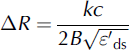
where k is a windowing factor and depends on the weighting function used and is the relative permittivity of dry snow. Each receive signal must be windowed to reduce spectral leakage, which manifests itself as range side-lobes in the data, resulting from the Fourier transform (Reference HarrisHarris, 1978). Choosing the appropriate window requires a trade-off between main-lobe widening, which results in degradation in range resolution, and suppression of side-lobes that could potentially mask normally resolvable, but weaker, targets of interest. The relative permittivity of dry snow can be expressed in terms of snow density, ρ _s, as (Reference Ulaby, Moore and FungUlaby and others, 1986a)

The vertical range resolution values listed in Table 1 and the depth axes in the figures assume a mean snow density of 0.3 g cm³ (Reference WarrenWarren and others, 1999; Reference MassomMassom and others, 2001; Reference Sturm, Holmgren and PerovichSturm and others, 2001) and a windowing factor of 2 (Reference HarrisHarris, 1978). Snow density on sea ice may increase/ decrease with depth, and, as a result, the depth axes may under-/overestimate, respectively, the depth for deeper layers. As detailed in Reference KwokKwok and others (2011), varying the snow density by 0.1 g cm⁻³ results in a 5% change in the velocity of propagation, or a ∼20 mm difference in the range resolution of the radar in snow.

Assuming a sufficiently smooth surface, the cross-track resolution is the diameter of the pulse-limited footprint. The radius of the pulse-limited footprint, r _pl, is defined as

where B is the bandwidth and h is the altitude above the surface (m). All the footprint diameters listed in Table 1 are calculated with a pulse-limited assumption at 500 m altitude (Reference Kingsley and QueganKingsley and Quegan 1999).

The along-track resolution is dependent on the synthetic aperture length formed through the hardware and software averaging and the altitude above the surface. The synthetic aperture length is dependent on the product of the hardware and software averaging of the data, 16 in this case, the velocity of the aircraft, and the PRF. The synthetic aperture length is defined as

where n is the product of the number of pre-sums (averages) done in hardware and software, v is the velocity of the platform, assumed to be 130 m s⁻¹, and the PRF is 2 kHz for normal operation. The half-power beamwidth for the synthetic aperture is defined as (Reference Ulaby, Moore and FungUlaby and others, 1986b)

where λ is the wavelength at the center frequency and L is the synthetic aperture length defined in Eqn (6). The along-track resolution can now be defined as

where H is the altitude above the surface and β is the half-power beamwidth defined in Eqn (7). All along-track resolutions listed in Table 1 assumed a 500 m altitude. Note that these along-track resolutions are coarser than that of the cross-track resolution, i.e. pulse-limited footprint. The pulse-limited footprint is based on the assumption that the surface is sufficiently smooth.

Processing

Data processing to generate a radar echogram to display returns from air/snow and snow/ice interfaces consists of six basic steps:

1. 1. Reduction of coherent noise generated from the direct antenna-to-antenna coupling;

2. 2. Phase correction and time shift to correct aircraft altitude variation;

3. 3. Integration to improve signal-to-noise ratio (SNR) and along-track resolution;

4. 4. Fourier-transforming of data to obtain radar response as a function of range;

5. 5. Incoherent integration to reduce fading effects and concatenating range lines to generate a radar echogram; and

6. 6. Processing of data from step 4 with an interface or layer tracker to estimate air/snow and snow/ice interfaces and converting the range difference between the two interfaces into snow thickness assuming a constant density.

Radar data are corrupted by unwanted coherent signals caused by the direct antenna-to-antenna coupling, referred to as coherent noise. Figure 6a shows an echogram over the Antarctic ice sheet showing multiple internal layers where the coherent noise restricts the useful data to the shallowest 10 m. The coherent noise present within the data manifests itself as dark, horizontal lines in the echogram. Figure 6b shows the range-Doppler domain of Figure 6a which shows that the coherent noise resides in the zero Doppler bin. These unwanted signals remain coherent over a sufficiently long duration that we are able to reduce them by ∼15 dB using an approach similar to that reported by Reference BeavenBeaven (1995). We coherently averaged a number of range lines to generate an estimate of the coherent noise. As expected, the averaging resulted in a reduction of return power from the air/snow interface and enhancement of the coherent noise. We then subtracted the averaged signal from each range line to reduce the coherent noise to obtain an improvement in the SNR. This processing step also removes the DC bias of the data due to hardware averaging. This does not affect snow returns as aircraft-induced motion results in non-zero Doppler when data are analyzed over a sufficiently large aperture. Figure 7 shows the same echogram as in Figure 6, after applying the coherent noise removal algorithm. The internal layering in this image is evident to at least 40 m beneath the surface.

Fig. 6.

(a) Radar echogram from 9 November 2009 Pine Island Glacier (Antarctica) flight which demonstrates the coherent noise present in the collected data which restricts useful data to the top 10 m. (b) The same data are displayed in the range-Doppler domain, and the strong zero-Doppler component can be clearly seen.

Fig. 7.

Snow Radar results from the 9 November 2009 Pine Island Glacier flight showing the improvement in SNR from the coherent noise removal method applied to the data in Figure 6a. A constant snow density of 0.3 g cm⁻³ was assumed. Firn snow density increases with depth, so the depth axes overestimate the depth for deeper targets.

Multiple steps take place prior to applying a fast Fourier transform (FFT) on the data to generate the FMCW radar response as a function of range. First, the GPS inertial navigation system (GPS/INS) data reference, typically the GPS antenna phase center, is transformed to the monostatic phase center of the radar antennas (the midpoint between the two antenna apertures). With the re-referenced GPS/INS data, a phase correction and time shift are performed to mitigate the effect of aircraft roll, pitch and yaw. The system response is then deconvolved, four additional averages are performed, which is analogous to an unfocused synthetic aperture radar (SAR) algorithm, and the data are Hanningwindowed for range side-lobe suppression. Every five range lines of the Fourier-transformed data are then incoherently averaged to reduce the data size for delivery to the US National Snow and Ice Data Center (NSIDC), where the data are archived and openly distributed to the science community. Decimation does not affect the quality of the processed data product because the spatial sampling of the data, which is on the order of 1 m and dependent upon aircraft velocity and PRF, is much less than the along-track footprint.

Snow thickness extraction, for now, relies upon threshold detection of both the air/snow and snow/ice interfaces and the underlying assumption that the magnitude of the return from the snow/ice interface is greater than that from the air/ snow interface (Reference KwokKwok and others, 2011; Reference FarrellFarrell and others, 2012). Relying on threshold detection implies relying upon the mean magnitude being above the noise floor for both interfaces, and, as a result, produces conservative snow thickness estimates; if the threshold for either interface is not exceeded, a snow thickness is not returned. As a reference, Reference KwokKwok and others (2011) reported 46%, 37% and 24% snow depth retrieval for the 31 March, 2 April and 5 April 2009 Arctic sea-ice flights. These percentages exclude the instances of open water and bare sea ice.

Results

Representative results for a sea-ice flight and land-ice flight are presented in this section. A more complete set of results is available through NSIDC (nsidc.org) and our CReSIS website (data.cresis.ku.edu). For all the echograms presented in this section, the depth, D, is found by converting the propagation delay (which is what the radar really measures) into range in snow using

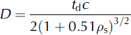
where t _d is the time delay between the air/snow interface and the target, and ρ _s is the density of dry snow (Reference Ulaby, Moore and FungUlaby and others, 1986a). As mentioned above, a mean snow density of 0.3 g cm⁻³ is used. Using a Taylor series expansion, the expression for calculating the percentage error of snow depth as a function of uncertainty in snow density is

For Δρ _s = ±0.1 g cm⁻³, the resulting percentage error in snow depth is ±16.63%. This error can be described as cumulative, as it increases for thicker snow cover.

Figure 8 shows a radar echogram generated for a 4 km segment from data collected over sea ice in the Bellingshausen Sea, Antarctica, on 23 October 2011. Air/snow and snow/ice interfaces are plotted in Figure 9a, with the extracted snow thickness vs spatial position shown in Figure 9b, and the associated histogram shown in Figure 9c indicates a range of depths from 40 to 150 cm, with a mean thickness of 93 cm. We omitted erroneous zero thickness results in computing the mean. Of particular interest is the pressure ridge seen at 0.6 km distance on the x-axis. The tracker described in the earlier section does not follow this pressure ridge along the top. There is also no clearly discernible snow/ice interface, indicating the existence of deformed ice. Another rough air/snow interface is seen from 1 to 1.4 km distance on the horizontal axis with a discernible snow/ice interface. The former is much more abrupt than the latter, and the weaker signal from the air/ snow interface can probably be attributed to increased surface roughness.

Fig. 8.

Snow Radar results from the 23 October 2011 Bellingshausen Sea ice flight. A constant snow density of 0.3 g cm⁻³ was assumed for deriving the depth axis.

Fig. 9.

Standard output from the interface tracker. (a) Extracted air/snow and snow/ice interfaces from the echogram presented in Figure 8. (b) Snow depth vs along-track position. (c) Histogram of snow thickness derived assuming a constant snow density of 0.3 g cm⁻³. Mean snow thickness for the segment was 93 cm.

Due to the heavy snow loading in the Antarctic, the second interface seen throughout Figures 8 and 9 is probably not the snow/ice interface. It is more likely a snow/slush interface as most of the sea ice is suppressed beneath the sea surface, causing in-flooding. This snow/slush interface has a stronger received signal power than the snow/ice interface, due to a larger dielectric contrast. Figure 10 shows a comparison between data collected over the Arctic (15 April 2011) and the Antarctic (23 October 2011) snow cover. Radar parameters for these two segments are given in Table 1; the only difference between the two segments is the transmit–receive antenna isolation. In general, second interface (snow/slush or snow/ice) returns are much stronger for the flight in Antarctica than those for the flight in the Arctic. To illustrate these differences, we plotted the radar response as a function of range, normally called A-scopes, on the right side of Figure 10. The red lines within the echograms show the spatial location of the range line used to produce the corresponding A-scope. Although the snow cover for the Antarctic sea-ice echogram is much more than that of the Arctic sea ice (>1 m vs 50 cm), the returns from the snow/ice interface, relative to those from the air/snow interface, in Antarctica are 12 dB larger than those obtained in the Arctic. These high values support that returns are from a snow/slush interface instead of a snow/ice interface. Reference Lytle, Jezek, Gogineni and HosseinmostafaLytle and others (1996) reported that the presence of slush resulted in an 8 dB higher return, at normal incidence, than that for a slush-free interface. The measurements by Reference Lytle, Jezek, Gogineni and HosseinmostafaLytle and others (1996) were performed with a coarse-resolution radar system operating at Ku-band frequencies and resulted in averaging over a much larger range window than the Snow Radar system.

Fig. 10.

Comparison between radar returns from the snow/ice interface for the Arctic (a) and Antarctic (b) sea ice. The second interface shown in echogram of (b) is believed to be a snow/slush interface due to the increase in the relative amplitude offset between the two interfaces.

As part of NASA OIB, the Snow Radar is operated on every flight regardless of altitude and targets of interest. Despite the low transmit power, at the nominal altitude of 500 m a.g.l. the radar is capable of detecting fine, near-surface accumulation layers on land ice to depths as great as 100 m, and consistently to depths of 20–40 m in the slower-moving dry snow zone. Figure 7 shows this capability for the 9 September 2011 Pine Island Glacier (Antarctica) flight with layers detected >40 m down from the apex of the surface. Compared to the varying densities of snow on sea ice, the snow density of firn generally increases with depth (range commonly 0.3–0.9 g cm⁻³), so using a single density of 0.3 g cm³ may overestimate the snow depth in deeper layers.

The range resolution of the system can be verified with data collected over bare sea ice, under the assumption that bare sea ice is a specular target for the radar. Reference Bredow and GogineniBredow and Gogineni (1990) investigated the backscattering coefficient vs incidence angle of a smooth saline ice sheet at C-band and reported a root-mean-square height of 0.029 cm, which satisfies the Fraunhofer criterion for smoothness at the center frequency of 5 GHz (Reference Ulaby, Moore and FungUlaby and others, 1986b). Radar returns from bare sea ice are noticeable due to the increase in side-lobe energy, which is evident for the entirety of the range window, and therefore suitable for deriving the system response. Two examples of this can be seen in Figure 11a. One instance is to the right of 1.60 km on the distance axis, and the other lies between 3.19 and 4.79 km on the distance axis; both instances are outlined with a red box.

Fig. 11.

Snow Radar results from the 16 March 2012 Beaufort–Chukchi flight in the Arctic. (a) Echogram for eight data files (Nos. 163–170) without compensating for the system response. (b) The same echogram with the system response deconvolved. (c) Comparison of the A-scopes at the location marked with the line. Average system response was derived from the A-scopes lying within the boxes outlined in (a).

Traditional deconvolution techniques are typically applied on data that have not been deramped, so the receive signal needs to be reramped. Reramping of the receive signal requires digitization of the transmit signal copy used to deramp the receive signal (Reference SoumekhSoumekh, 1999). This is not economical due to the sampling frequency requirement of the ADC to directly sample the 2–8 GHz chirp input to the LO port of the receive mixer to perform the reramping. As an alternative approach, an inverse filter (Reference Robinson and TreitelRobinson and Treitel, 2000) can be synthesized and applied to the data. An example of the output of the synthesized filter can be seen in Figure 11 b and c where the SNR improved by 5 dB and the range resolution, taken as the 6 dB lobe width of snow/ice interface, is ∼5.5 cm.

Conclusions

We have presented a high-level overview of the principle of operation of FMCW radars, a hardware description and processed data for a 2–8 GHz UWB, FMCW radar developed at CReSIS, known as the Snow Radar. When operating with standard parameters, the Snow Radar can provide a vertical range resolution of ∼5 cm in snow. Processed data from the first seven NASA OIB campaigns show that the Snow Radar can consistently resolve and detect the snow layer over sea ice. We also showed an example of firn on glacial ice where multiple accumulation layers were identified.

Snow depth retrievals have been compared to previous climatological values (Reference Kurtz and FarrellKurtz and Farrell, 2011) and to in situ measurements (Reference FarrellFarrell and others, 2012). Snow Radar data are currently being used in determination of sea-thickness (Reference KurtzKurtz and others, 2011), with the subsequent results used for sea-ice forecasting (Reference LindsayLindsay and others, 2012). In addition to this work, ongoing work on accurate snow depth retrievals will continue. Modeling of backscatter from the snow/sea-ice stratigraphy will be used to simulate responses that can be fit to the data to extract geophysical parameters of the snow and sea ice, such as density of snow and surface roughness of the air/snow and snow/ice interfaces.

We are currently developing an automated tracking algorithm that searches for the air/snow interface based upon a user-defined threshold above the noise power. Range compensation is then performed from this range bin and beyond. The snow/ice interface is taken to be the peak with the largest magnitude. Both interfaces are then weighted by their respective scattering magnitude and filtered over an 8–16 range line aperture to reduce tracker errors caused by low SNR. A surface classification algorithm to discriminate between snow cover, bare sea ice and open water is also under development. The algorithm is based on the roll-off from the peak response or the rise in the side-lobe energy over bare sea ice.

Future hardware development includes the design of a multi-channel receiver and antenna array to allow for three-dimensional (3-D) imaging of the air/snow and snow/ice interfaces on sea ice, in addition to 3-D imaging of the firn on land ice. We also plan to include a dual-polarization and quad-polarization cross-track array (Reference Kindt, Kragalott, Parent and TavikKindt and others, 2009) for operating the Snow Radar and a Ku-band altimeter together to measure radar backscatter as a function of incidence angle at a wide range of frequencies between 2–8 and 12–18 GHz. This is to estimate snow density from radar data using an approach similar to that reported by Reference RottRott and others (2010) without the need for extensive in situ snow characterization observations to convert radar-determined electrical range to snow thickness.