1. Introduction
Atomisation is a process that converts bulk liquids into fine droplets and has a number of applications, including spray combustion, spray painting, spray drying, agricultural sprays and inkjet printing (Lefebvre & McDonell Reference Lefebvre and McDonell2017). The goal of any atomisation process is to achieve the desired drop size distribution, which involves selecting the appropriate nozzle geometry and controlling the flow parameters. One of the common methods to atomise liquids is to force thin liquid sheets at high speeds, which causes the sheet to oscillate and break up. The break-up of the sheet is attributed to the Kelvin–Helmholtz instability, wherein a small, wavy perturbation introduced into the sheet is amplified through interactions between the liquid sheet and the surrounding gas phase.
Squire (Reference Squire1953) was the first to analyse the problem by performing a linear stability analysis for a constant thickness (
 $h$
), inviscid liquid sheet surrounded by an inviscid gas phase. He showed that, while both symmetric (varicose/dilational) and anti-symmetric (sinuous) waves are unstable, the growth rates for the sinuous waves are significantly higher than those for varicose waves. For thin liquid sheets moving in air, where
 $kh\ll 1$
, the condition for temporal instability for the sinuous mode is given by (Squire Reference Squire1953),
 \begin{align} \textit{We} \gt 2+\frac {kh}{\delta }, \end{align}
where
 $k$
is the wavenumber,
 $\sigma$
is the surface tension,
 $\delta = \rho _{{g}}/\rho _{{l}}$
is the ratio of gas to liquid density and the Weber number,
 $\textit{We} \equiv \rho _{{l}} U^2 h/ \sigma \gg 1$
measures the competition between the inertial and surface tension forces. Here,
 $U$
is the liquid’s speed, assumed constant across the sheet thickness. Clearly, if the aerodynamic effects are ignored (
 $\rho _g = 0$
), the moving liquid sheet is stable to all infinitesimal perturbations. It should, however, be noted that sheets can be destabilised in the absence of aerodynamic effects, such as in the case of large deformations of the interface involving inertia and surface tension, as demonstrated by Burton & Taborek (Reference Burton and Taborek2007), or for small deformations in very thin films, of the order of tens of Angstroms, when the van der Waals force competes against viscous and surface tension forces to rupture the sheet (Ruckenstein & Jain Reference Ruckenstein and Jain1974; Vaynblat, Lister & Witelski Reference Vaynblat, Lister and Witelski2001).
Following Gaster (Reference Gaster1962), who showed that the temporal growth rate could be related to the spatial growth rate via the group velocity, Asare, Takahashi & Hoffman (Reference Asare, Takahashi and Hoffman1981) used the results of the temporal analysis of Squire (Reference Squire1953) to derive an expression for the critical forcing frequency below which the sheet is stable to perturbations (
 $\delta \ll \tanh (kh/2))$
 \begin{align} \omega _{{c}} \approx \frac {\rho _{{g}} U^3}{\sigma }. \end{align}
They experimented with planar water sheets issuing vertically downward from slit nozzles and obtained images of the spatially evolving sinuous waves. When the slit nozzle was vibrated at amplitudes much smaller than the sheet thickness and at forcing frequencies below the critical value, excellent agreement was found between the predicted and observed growth rates for
 $\textit{We}=548$
(their
 $\textit{We}$
is based on the half-thickness). The normalised wave envelopes overlapped for increasing forcing amplitudes at fixed forcing frequency, except that the break-up occurred at shorter fall distances for higher amplitudes, which was attributed to nonlinear effects. Decreasing the surrounding air pressure reduced spatial growth due to weaker aerodynamic interactions. Interestingly, in experiments performed at forcing frequencies above the critical value, sinuous waves were also observed to grow near the nozzle and then stabilise after a short fall distance. The former was attributed to the initial transverse momentum imparted to fluid particles leaving the vibrating nozzle and not due to an instability.
While the aforementioned study reported close agreement with Squire’s theory, a more recent set of experiments performed by Tammisola et al. (Reference Tammisola, Sasaki, Lundell, Matsubara and Söderberg2011) on an identical geometry and similar sheet thickness but for slightly higher Weber number (
 $\textit{We}=700$
) showed that the measured spatial growth rates is approximately half to one-third of the predicted value. The reduced growth rate is attributed to the presence of the gas boundary layer next to the liquid sheet, which reduces the effective velocity difference between the liquid and the surrounding gas phase. An Orr–Sommerfield equation results from a locally parallel assumption and predicts the reduced growth rates, due to the presence of the boundary layer, in close agreement with their measurements. They also varied the gas velocity to show that the instability decreases when the velocity difference between the sheet and the surrounding gas phase is reduced.
The aerodynamic theory of Squire has been applied to explain the dynamics of a radially expanding liquid sheet produced by the impact of two co-axial opposing jets or a jet impinging co-axially with a cylindrical impactor (Taylor Reference Taylor1959; Weihs Reference Weihs1978). The dynamics of the circular sheet is characterised by the jet Weber number,
 $\textit{We}_{{d}}=\rho _{{l}} U^2 d_{\!{j}}/\sigma$
, where
 $d_{\!{j}}$
is the jet diameter and
 $U$
is the jet speed. At low
 $\textit{We}_{{d}}$
, the sheet is smooth with its diameter set by a balance between the inertial force stretching the sheet and the retarding force of the surface tension at the rim. Taylor (Reference Taylor1959) has shown that when a steady, point (sinuous) perturbation is introduced at the centre, the stationary perturbation forms a cardioid on the sheet with a magnitude that diverges at the edge of the sheet. Importantly, the amplification in sinuous perturbation takes place in the absence of any aerodynamic disturbance. Huang (Reference Huang1970) has shown that, while the sheet produced from two colliding co-axial jets is smooth for
 $\textit{We}_{{d}} \lesssim 800$
, small perturbations originating at the colliding point for higher Weber numbers (
 $\textit{We}_{{d}}=$
800–2000) propagate radially with increasing amplitude. This growth in the transition regime is attributed to the cardioidal waves and occurs in the absence of any aerodynamic interactions. For
 $\textit{We}_{{d}}\gt 2000$
, the sheet is distinctly unstable and starts to flap. Increasing
 $\textit{We}_{{d}}$
increases the instability, causing the sheet diameter to decrease as
 $\textit{We}_{{d}}^{-1/3}$
. Huang (Reference Huang1970) attributed the decrease to the aerodynamic interactions and employed the dispersion relation of Squire to confirm the observations.
Bremond, Clanet & Villermaux (Reference Bremond, Clanet and Villermaux2007) investigated the stability of radially expanding liquid sheets when the impactor is vibrated at varying amplitudes and frequencies. Following Asare et al. (Reference Asare, Takahashi and Hoffman1981), they predict a critical/cutoff frequency for each Weber number, beyond which the circular sheet becomes stable. They observed spatial growth for both stable and unstable forcing and distinguished the two cases by tracking the position of the first antinode of the wave envelope. For stable forcing (
 $\omega \gt \omega _{{c}}$
), the position of the antinode did not vary significantly, which they attributed to the most unstable mode (and not to that corresponding to the forcing frequency). Variations in the position of the first antinode were observed for frequencies below the critical value, and the change in location of the first antinode with frequency was attributed to the aerodynamic instability at a mode corresponding to the forcing frequency. Interestingly, the spatial growth rates were similar for both stable and unstable forcing (see their figure 14).
In contrast to the aforementioned studies, Tirumkudulu & Paramati (Reference Tirumkudulu and Paramati2013) derived the governing equations for the dynamics of a sinuous wave on a radially expanding liquid sheet in the absence of aerodynamic interactions. The derivation followed that for a liquid curtain (Weinstein et al. Reference Weinstein, Clarke, Moon and Simister1997) and predicted the liquid sheet to be unstable to all forcing frequencies, with the perturbation diverging at the edge of the sheet. The predictions of the model showed good agreement with the slope of the sinuous perturbation under varying forcing frequencies and amplitudes, including those performed under low gas pressure (Majumdar & Tirumkudulu Reference Majumdar and Tirumkudulu2018). However, Mehring & Gyurkovich (Reference Mehring and Gyurkovich2023) have recently shown that the original derivation of Tirumkudulu & Paramati (Reference Tirumkudulu and Paramati2013) ignored a term in the kinematic boundary condition, which, on inclusion, eliminates the instability. However, Tirumkudulu (Reference Tirumkudulu2023) shows that the modified equations predict that the amplitude of the sinuous perturbation will grow spatially. The perturbations diverge at the edge of the sheet across a finite range of frequencies and for finite slope of the perturbation at the point of impingement. The varicose mode, on the other hand, decays inversely with radial distance at this order of approximation.
The goal of the present work is to reassess the range of applicability of the modified equations (Mehring & Gyurkovich Reference Mehring and Gyurkovich2023; Tirumkudulu Reference Tirumkudulu2023) by comparing the model predictions with the existing experimental results and whether a finite perturbation slope at the impingement point can indeed explain the observed spatial growth of the sinuous mode. We first show that a finite-slope perturbation of zero frequency at the point of impingement causes the sinuous perturbation to diverge logarithmically at the edge of the sheet. As the frequency is increased, the wave envelope follows the growth profile observed for zero frequency (steady perturbation), with the first antinode aligning with the zero-frequency curve, and all subsequent antinodes exhibiting no further growth. We next compare the predictions of the modified model with measurements. Here, we show that a small slope of the sinuous mode at the point of impingement caused by noise in the system can result in sinuous modes close to those observed in experiments. Importantly, the non-zero slope necessary to match the observations is of very small magnitude,
 $\mathcal{O}(0.01^{\circ }{-}0.1^{\circ })$
, thereby emphasising the role of noise in inducing spatial growth.
2. Problem statement
A radially expanding liquid sheet is formed when two laminar liquid jets (of speed
 $U$
and diameter
 $d_{\!{j}}$
) impinge head on, or when a single jet impacts a cylindrical impactor (figure 1). If there is negligible energy loss at the point of impingement, the radial velocity, to the lowest order, is equal to the speed of the jet. The thickness of the sheet for the two-jet assembly, at any location
 $r$
, is derived from a simple mass,
 $h(r) = d_{\!{j}}^2/ 4r$
(Tirumkudulu & Paramati Reference Tirumkudulu and Paramati2013). A radial momentum balance at the edge of the sheet sets the radial extent of the sheet (
 $R_{{t}}$
) in terms of the local thickness (
 $h_{{t}}$
),
 $2\pi R_{{t}} h_{{t}} U^2 \rho _{{l}} = 2 \times 2 \pi R_{{t}} \sigma$
, which in turn sets the value of the local Weber number at the edge of the sheet,
 $ \textit{We}_{{h}}=\rho _{{l}} U^2 h_{{t}}/ \sigma =2$
(Taylor Reference Taylor1959).
Schematic of the radially expanding liquid sheet formed by head-on impingement of two equal collinear liquid jets.

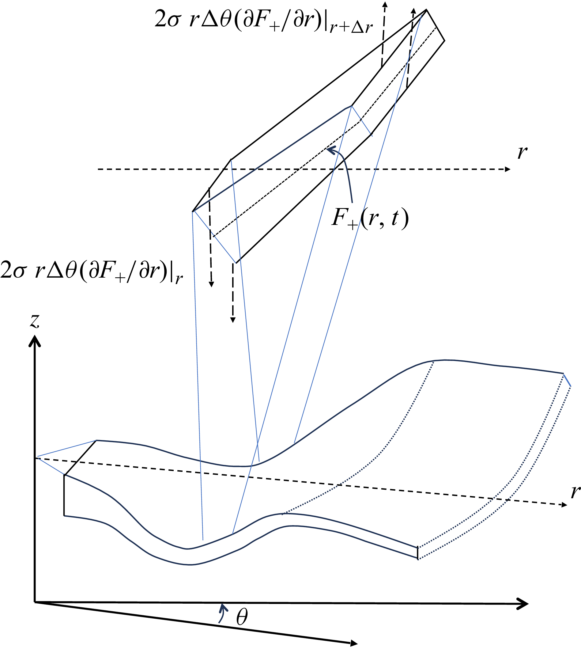
A schematic of the deforming sheet and a sectional element of the sheet showing the vertical component of surface tension force acting on the sheet.

The governing equation for the dynamics of the centreline of the liquid sheet (equivalently, the sinuous-mode perturbation) may be derived from a vertical force balance (figure 2). The vertical velocity of a fluid element moving at speed
 $U$
in the radial direction at any time,
 $t$
, is given by
 \begin{align} v_z(r,t) = \left (\frac {\partial }{\partial t} + U\frac {\partial }{\partial r} \right )F_+(r,t) , \end{align}
while the acceleration in the vertical direction is given by,
 \begin{align} a_z(r,t) = \left (\frac {\partial }{\partial t} + U\frac {\partial }{\partial r} \right )^2 F_+(r,t) . \end{align}
Here,
 $F_+$
is the position of the sheet centreline and represents the sinuous mode. Equating the mass times vertical acceleration of a section of the sheet of local thickness,
 $h$
, and of span
 $r \Delta \theta \Delta r$
to the surface tension (
 $\sigma$
) force results in the following shell balance:
 \begin{align} \rho _{{l}} h r \Delta \theta \Delta r \left (\frac {\partial }{\partial t} + U\frac {\partial }{\partial r} \right )^2 F_+ = \left (2 \sigma r \Delta \theta \frac {\partial F_+}{\partial r}|_{r + \Delta r} - 2 \sigma r \Delta \theta \frac {\partial F_+}{\partial r}|_{r} \right )\! . \end{align}
Note that, here, the arc length used to calculate the mass of the sheet element is written in terms of
 $\Delta r$
by invoking the small-slope approximation, under which the radial derivative of the displacement remains much smaller than unity. In this limit, the arc length of the sheet element differs negligibly from its radial projection, and higher-order geometric corrections can be safely neglected.
The time-dependent equation for the sinuous mode is obtained by dividing throughout by
 $\Delta \theta \Delta r$
and taking the limit,
 $\Delta r \rightarrow 0$
 \begin{align} \rho _{{l}} h r \left (\frac {\partial ^2 F_+ }{\partial t^2} + 2 U\frac {\partial ^2 F_+ }{\partial r \partial t} + U^2 \frac {\partial ^2 F_+ }{\partial r^2} \right ) = 2 \sigma \frac {\partial }{\partial r} \left ( r\frac {\partial F_+}{\partial r} \right )\! . \end{align}
In passing, we note that Weihs (Reference Weihs1978) performed a similar force balance that also included viscous deformation and aerodynamic interaction. However, the acceleration of the fluid element was obtained from the time derivative of the fluid element instead of its material derivative. Consequently, his force balance misses the second and third terms on the left-hand side in the above equation.
The dimensionless form of the above equation is obtained using the following scaling:
 \begin{align} r \sim R; \;\; h, F_+ \sim H; \;\; t \sim R/U\, , \end{align}
giving (Mehring & Gyurkovich Reference Mehring and Gyurkovich2023; Tirumkudulu Reference Tirumkudulu2023)
 \begin{equation} \frac {1}{\textit{We}_{{H}}} \bigg [\frac {1}{\bar {r}} \frac {\partial }{\partial \bar {r}} \bigg (\bar {r} \frac {\partial \bar {F}_+}{\partial \bar {r}} \bigg )\bigg ] = \frac {1}{2\bar {r}} \bigg ( \frac {\partial ^2 \bar {F}_+}{\partial \bar {t}^2 } + 2\frac {\partial ^2 \bar {F}_+}{\partial \bar {t} \partial \bar {r} } + \frac {\partial ^2 \bar {F}_+}{\partial \bar {r}^2 } \bigg ). \end{equation}
Here,
 $H$
is the characteristic thickness at a characteristic radial location
 $R$
, and
 $\textit{We}_{{H}} = \rho _{{l}} U^2 H/\sigma$
is the Weber number calculated with respect to the characteristic thickness.
The edge of the circular sheet in the dimensionless form is given by
 $\bar {r} = {\textit{We}_{{H}}}/{2}$
. We will henceforth use (2.6) in the current work and refer to this as the ‘modified thinning’ theory to distinguish it from the thinning theory originally proposed by Tirumkudulu & Paramati (Reference Tirumkudulu and Paramati2013). The details of the modification made can be found in Mehring & Gyurkovich (Reference Mehring and Gyurkovich2023) and Tirumkudulu (Reference Tirumkudulu2023).
An important result in Tirumkudulu (Reference Tirumkudulu2023), which requires emphasis, is that, when a constant displacement (or a zero-frequency perturbation) is introduced at the point of impingement, the governing equation for the spatial evolution of the steady perturbation is given by
 \begin{equation} \left (\frac {\textit{We}_{{H}}}{2} -\bar {r} \right ) \frac {\partial ^2 \bar {F}_+}{\partial \bar {r}^2} - \frac {\partial \bar {F}_+}{\partial \bar {r}}=0 . \end{equation}
On integrating the above equation, we obtain the slope of the perturbation
 \begin{equation} \frac {\partial \bar {F}_+}{\partial \bar {r}} = \frac {A}{\displaystyle \left ( \frac{\textit{We}_{{H}}}{2}-\bar {r} \right )}\! , \end{equation}
while a second round of integration gives the spatial evolution of the perturbation
 \begin{equation} \bar {F}_+ = B - A \ln\! \left (\frac {\textit{We}_{{H}}}{2} - \bar {r}\right )\! . \end{equation}
Here,
 $A$
and
 $B$
are constants of integration. For non-zero slope (
 $A\ne 0$
), the perturbation diverges logarithmically at the edge of the sheet. On the other hand, a zero-slope perturbation does not grow.
If azimuthal variation is included in (2.7), Taylor (Reference Taylor1959) has shown that a perturbation (superposition of small cardioid perturbations) introduced close to the point of impingement will diverge even more strongly at the edge of the sheet irrespective of the slope of the perturbation at the impingement point
 \begin{align} \bar {F}_+ = A \!\left ( \frac {\bar {r}}{\frac{\textit{We}_{{H}}}{2} - \bar {r}} \right )^{1/4}\! . \end{align}
In this study, we shall consider only axisymmetric perturbations, where sinusoidal sinuous perturbations are introduced close to the impingement point, and seek solutions of the form
 \begin{equation} \bar {F}_+(\bar {r},\bar {t}) = \bar {S}(\bar {r}) e^{i\bar {\omega }\bar {t}} . \end{equation}
Our goal is to determine the spatial evolution of
 $\bar {S}(\bar {r})$
for varying forcing frequencies and perturbation amplitudes and slopes.
Substituting the above form of the solution in (2.6), we obtain the governing equation for the sinuous mode
 \begin{equation} \bigg (\frac {1}{2} - \frac {\bar {r}}{\textit{We}_{{H}}} \bigg ) \frac {\text{d}^2 \bar {S}}{\text{d} \bar {r}^2} = \bigg ( - i\bar {\omega } + \frac {1}{\textit{We}_{{H}}} \bigg ) \frac {\text{d} \bar {S}}{\text{d} \bar {r} } + \frac {\bar {\omega }^2}{2} \bar {S}\, . \end{equation}
The system is described by the following boundary conditions:
 \begin{align} \bar {F}_+(\bar {r}_0,\bar {t}) = \frac {a_0}{H} e^{i\bar {\omega } \bar {t}}, \quad \left .\frac {\partial \bar {F}_+}{\partial \bar {r}}\right |_{\bar {r}=\bar {r}_0} = \frac {\text{d}S^0} {H/R} e^{i\bar {\omega } \bar {t}}, \end{align}
so that the boundary conditions for (2.12) become
 \begin{equation} \bar {S}(\bar {r}_0) = \frac {a_0}{H}, \left .\frac {\text{d} \bar {S}}{\text{d} \bar {r} }\right |_{\bar {r}=\bar {r}_0} = \frac {\text{d}S^0} {H/R}. \end{equation}
Here,
 $\bar {r}_0$
denotes a small radial distance from the impingement point where a perturbation of amplitude
 $a_0$
and slope
 $\text{d}S^0$
is introduced.
Equation (2.12) is a second-order, linear ordinary differential equation governing the spatial evolution of the sinuous-mode amplitude for a prescribed forcing frequency. Since the objective of the present work is to determine spatial growth, the forcing frequency is specified a priori and the equation is solved by marching radially outward from a small but finite location near the impingement point. Both the displacement amplitude and its slope are prescribed at this location, rendering the problem well posed.
The governing equation is recast as an equivalent system of first-order ordinary differential equations and solved numerically in MATLAB® using the solver ode45, which is based on a Runge–Kutta scheme. Care is taken to terminate the integration before reaching the sheet edge, where the governing equation becomes singular as
 $\bar {r} \rightarrow {\textit{We}_{{H}}}/2$
. The spatial envelope of the perturbation is then obtained from the magnitude of the complex solution.
3. Comparison of the predictions of the modified thinning theory with experiments
We shall compare the experimental results of Bremond et al. (Reference Bremond, Clanet and Villermaux2007), Paramati, Tirumkudulu & Schmid (Reference Paramati, Tirumkudulu and Schmid2015), Majumdar & Tirumkudulu (Reference Majumdar and Tirumkudulu2018), Dighe & Gadgil (Reference Dighe and Gadgil2019) and Gyurkovich & Mehring (Reference Gyurkovich and Mehring2023) with the predictions of the theory. Before moving forward, it is useful to familiarise ourselves with the experimental set-ups and the methods of forcing applied in each of the five cases.
Paramati et al. (Reference Paramati, Tirumkudulu and Schmid2015) formed a radially expanding liquid sheet by head-on impingement of two liquid jets each of diameter 1.62 mm. Acoustic perturbation was applied near the impingement point using a high-intensity acoustic speaker. The frequency of the perturbation was controlled using a function generator and the perturbation amplitude was varied in terms of the sound pressure level (SPL) using an amplifier. Note that the actual perturbation amplitude of the liquid sheet applied at the impingement point is not known, since the forcing was acoustic in nature and the displacement of the impingement point was not measured.
Bremond et al. (Reference Bremond, Clanet and Villermaux2007), Majumdar & Tirumkudulu (Reference Majumdar and Tirumkudulu2018) and Gyurkovich & Mehring (Reference Gyurkovich and Mehring2023) employed jet-on-impactor set-ups. Liquid jets of diameters 2.9, 2.5 and 3 mm, respectively, impinge head on with circular impactors of diameters 6, 9 and 10 mm, respectively. In studies by Bremond et al. (Reference Bremond, Clanet and Villermaux2007) and Gyurkovich & Mehring (Reference Gyurkovich and Mehring2023), the impactor was perturbed using a shaker system, which allowed independent control of the perturbation frequency and amplitude, applied exclusively at the impingement point. Majumdar & Tirumkudulu (Reference Majumdar and Tirumkudulu2018) mounted the impactor on a speaker, which was connected to a function generator and a sound amplifier and achieved independent control of amplitude and frequency, similar to that in the previous two studies.
Dighe & Gadgil (Reference Dighe and Gadgil2019) conducted experiments on a liquid sheet shaped like a bay leaf, created by the oblique impingement of two 1 mm diameter liquid jets at a
 $90^\circ$
angle. The liquid sheet was perturbed via acoustic forcing applied using a speaker, and the signal frequency and SPL were controlled using a sine wave generator and an amplifier, similar to the experiments of Paramati et al. (Reference Paramati, Tirumkudulu and Schmid2015).
Since the thinning theory was initially derived for head-on impingement of two jets, modifications are needed to account for a single-jet-impactor assembly. For two impinging jets, the thickness of the sheet is
 $h(r) = d_{\!{j}}^2/4r$
for head-on collision, while
 $h(r) = d_{\!{j}}^2/0.7r$
for the bay-leaf sheet (Dighe & Gadgil Reference Dighe and Gadgil2019). For a single-jet configuration, the sheet thickness variation is given by,
 $h(r) = d_{\!{j}}^2/8r$
. This affects how we define the characteristic thickness
 $H$
at the characteristic location
 $R$
, namely,
 $H = d_{\!{j}}^2/4R$
for coaxial double jets,
 $H = d_{\!{j}}^2/0.7R$
for double jets colliding at
 $90^\circ$
and
 $H = d_{\!{j}}^2/8R$
for the jet-on-impactor configuration. The theoretical sheet break-up radius (
 $R_{\kern-1pt t}$
) under smooth flow conditions for the coaxial two-jet configuration is
 $R_{\kern-1pt t}/d_{\!{j}}= \textit{We}_{{d}}/8$
while that for a single jet impacting an impactor is given by
 $R_{\kern-1pt t}/d_{\!{j}} = \textit{We}_{{d}}/16$
. In the following study, we have taken
 $R = R_{\kern-1pt t}$
so that
 $H$
corresponds to the film thickness at the edge of the sheet and the dimensionless radial coordinate,
 $\bar {r}$
, varies from 0 to 1. Consequently, the Weber number defined with respect to the film thickness becomes
 $\textit{We}_{{H}}=2$
.
When comparing measurements with predictions (2.12) and (2.14) for cases where the jet impinges on a vibrating impactor,
 $r_0$
corresponds to the impactor’s radius, and
 $a_0$
is the impactor’s vibration amplitude. For the two-jet impingement case, when the impingement point is displaced via acoustic forcing,
 $r_0$
is the radius of the jet while
 $a_0$
is chosen so that the first measured displacement point of the sheet matches the prediction.
3.1. Comparison of theoretical predictions with the experiments of Bremond et al. (Reference Bremond, Clanet and Villermaux2007) and Gyurkovich & Mehring (Reference Gyurkovich and Mehring2023)
We first compare the predictions of the thinning theory with the experiments conducted by Bremond et al. (Reference Bremond, Clanet and Villermaux2007) and Gyurkovich & Mehring (Reference Gyurkovich and Mehring2023). Gyurkovich & Mehring (Reference Gyurkovich and Mehring2023) have recently reported experiments performed in a parameter regime close to that of Bremond et al. (Reference Bremond, Clanet and Villermaux2007) and these measurements give an indication of the variation that can be expected between experiments performed under similar conditions.
At low Weber numbers
 $(\sim 320)$
, which correspond to the smooth regime, and at a forcing frequency of 150 Hz, both studies report no spatial growth. The spatially evolving perturbation envelope is compared with predictions of the modified thinning theory and good agreement is found, see figure 3. Specifically, there is good match both in the amplitude and location of the first antinode, and there are only small differences in the location and magnitude of the subsequent nodes and antinodes.
Comparison of experimental growth with the modified thinning theory for
 $f = 150$
Hz.

Similarly, experiments by Gyurkovich & Mehring (Reference Gyurkovich and Mehring2023) at
 $\textit{We}_{{d}} = 540$
(smooth regime) for forcing frequencies of 110 and 80 Hz, and the latter for three different amplitudes, show no spatial growth. Again, the predictions of the modified thinning theory match well with measurements; the location and amplitude of the initial few nodes and antinodes are somewhat close to the predictions (figure 4). These results suggest that the modified thinning theory accurately predicts the behaviour of the sheet for the smooth regime. We note that these comparisons have also been demonstrated recently by Gyurkovich & Mehring (Reference Gyurkovich and Mehring2023).
Comparison of experimental growth with the modified thinning theory at
 $\textit{We}_{{d}} = 540$
for (a)
 $f = 110$
Hz and (b)
 $f = 80$
Hz.

Measurements and experiments for
 $\textit{We}_{{d}} = 850$
. (a) Dimensionless sinuous perturbation plotted as a function of radial distance for five different forcing frequencies. Measurements are from the study of Bremond et al. (Reference Bremond, Clanet and Villermaux2007). (b) Predicted dimensionless sinuous perturbation for zero initial slope plotted as a function of radial distance for the same five different forcing frequencies as in (a). (c) Predicted dimensionless sinuous perturbation for finite initial slope plotted as a function of radial distance for various low-frequency perturbations (
 $f_2$
) along with the data of (a). (d) Predicted dimensionless sinuous perturbation for finite initial slope plotted as a function of radial distance for a linear combination of low-frequency noise (
 $f_2$
) along with that for the forcing frequency (
 $f_1=260$
Hz). The prediction is compared against the measurements of Bremond et al. (Reference Bremond, Clanet and Villermaux2007) and Gyurkovich & Mehring (Reference Gyurkovich and Mehring2023).

Next, we consider the case of higher Weber numbers. Figure 5(a) plots the measured envelope by Bremond et al. (Reference Bremond, Clanet and Villermaux2007) for the sinuous mode for
 $\textit{We}_{{d}}=850$
for various forcing frequencies. The magnitude of the first antinode for the lowest frequency (140 Hz) is the highest compared with the other frequencies, and the first antinode is located farther along the radial coordinate compared with those at higher frequencies. As the frequency is increased to 180 and 220 Hz, both the magnitude and location of the first antinode decrease, although the amplification follows a trend similar to that observed for 140 Hz. With further increase in forcing frequency (240 and 260 Hz), amplification is identical, but there is no significant change in the location or the amplitude of the first antinode. Bremond et al. (Reference Bremond, Clanet and Villermaux2007) use this invariance in location and amplitude of the first antinode to identify the critical frequency. Recall that the latter is defined as the frequency below which the perturbation is amplified at the forcing frequency via the Squire instability while above it, the sheet is stable to the forcing frequency. But since the amplification is observed at all frequencies, it is hypothesised that growth in the case of stable forcing is caused by the most unstable mode present in the noise, whose frequency is lower and different from the forcing frequency. As we shall see next, the changes in the location of the antinode with frequency emerge naturally from the dynamics described by the modified thinning equation.
We investigate whether the modified thinning theory is capable of explaining the observed amplification and position of antinodes for the higher Weber numbers. For the aforementioned frequencies at
 $\textit{We}_{{d}} = 850$
, figure 5(b) plots the envelope predicted by the modified thinning theory, which ignores the aerodynamic interactions. There is zero growth in all cases, but the location of the first antinode shows a trend similar to that observed in experiments in that the antinodes are spaced further apart for lower frequencies but closely overlap for the higher frequencies. Thus, the criteria for distinguishing stable and unstable frequencies using the Squire theory emerge naturally in the present analysis.
The aforementioned analysis has assumed that the slope of the disturbance (
 $\text{d}F_+/\text{d}r$
) is zero at the point of impingement. While the assumption appears reasonable, we investigate whether small, low-frequency disturbances of finite slope inherent to an experimental system can lead to the spatial growths observed in experiments. The disturbances may be of the nature described by Huang (Reference Huang1970) that originate at the colliding point of the jet(s) at higher Weber numbers and propagate throughout the entire sheet. These disturbances may also exist at lower Weber numbers, but they are expected to be small and hence do not prevail. Crapper & Dombrowski (Reference Crapper and Dombrowski1984) have also highlighted the effects of inherent noise in the experimental set-up on the liquid sheet. They show that a combination of high-frequency disturbances in the tubing connecting the nozzles and low-frequency disturbances from machinery in the building and the rig’s resonance significantly altered the wave dynamics. Alternatively, some researchers have proposed that impact waves, generated by the collision of two liquid jets or by the collision of a liquid jet with a solid impactor, contribute to the growth of instabilities (Dombrowski & Hooper Reference Dombrowski and Hooper1963; Ryan et al. Reference Ryan, Anderson, Pal and Santoro1995; Dighe & Gadgil Reference Dighe and Gadgil2018). In the case of two impinging jets, Dombrowski & Hooper (Reference Dombrowski and Hooper1963) identified the presence of a critical Weber number, above which the impact waves dominate, driving the growth of sinuous waves, while Anderson et al. (Reference Anderson, Ryan, Harry and Santoro2006) suggests that the impact waves could generate a spectrum of disturbances.
To this end, we plot the envelope predicted by the modified thinning theory for low frequencies (
 $f_2$
) ranging from 0 to 20 Hz for a finite value of initial slope (
 $\text{d}\bar {F}_+/\text{d}\bar {r} = 17$
) at the edge of the impactor (figure 5
c). The dimensional value of the slope is 0.00075, which corresponds to a very small angle of 0.0429
 $^{\circ }$
, and is of the same order as
 $\textrm{d}h/\textrm{d}r$
. Figure 5(c) shows that the position of the first antinode follows the spatial growth of the steady disturbance (at least for frequencies below 10 Hz). These results suggest that low-frequency noise with a small but finite slope can exhibit growth rates close to those observed in experiments.
Figure 5(d) plots the experimental results of both Bremond et al. (Reference Bremond, Clanet and Villermaux2007) and Gyurkovich & Mehring (Reference Gyurkovich and Mehring2023) performed under identical conditions. While Bremond et al. (Reference Bremond, Clanet and Villermaux2007) extracted the shape of the envelope by overlapping images of a section of the liquid sheet lit by a laser sheet, Gyurkovich & Mehring (Reference Gyurkovich and Mehring2023) used a chromatic confocal measurement technique, which detects the vertical position of the upper and lower interfaces at a fixed radial location. First, we notice that the peak values of the two experiments do not match; in fact, there is a large difference in the amplitude of the first antinode. Next, the locations of the first antinodes and the nodes are similar, although the positions of the subsequent nodes and antinodes show differences. These results indicate that variations in measurements obtained from different set-ups but under identical conditions may be due to inherent noise in the system. There is, however, similar growth in the amplitude of the envelope.
Figure 5(d) also includes the predicted envelope for a linear combination of perturbations for the forcing frequency and that for a low-frequency noise (1 Hz) at a finite slope
 \begin{equation} \bar {F}_+(\bar {r},\bar {t}) = \bar {S}_1(\bar {r}) e^{i\bar {\omega _1}\bar {t}} + \bar {S}_2(\bar {r}) e^{i\bar {\omega _2}\bar {t}}. \end{equation}
Here,
 $\bar {\omega _{\!j}} \equiv \omega R/U$
is the dimensionless frequency and
 $\bar {S}_{\!j} \equiv S_{\!j}/H$
is the dimensionless displacement with
 $j = 1$
and
 $j = 2$
corresponding to the values for forced perturbation and the inherent low-frequency noise, respectively. The boundary conditions are
 $\bar {S}_{\!j}(r_0) = a_{\!j}/H$
and
 $\text{d}\bar {S}_{\!j}/\text{d}\bar {r}|_{r_0} = \text{d}\bar {S}^0_{\!j}$
, which scales as
 $\sim H/R$
. We set the slope of the forced perturbation as zero (
 $\text{d}\bar {S}^0_1 = 0$
), since it is the growth of the inherent low-frequency noise that contributes to the growth of the sheet, and the amplitude of the inherent disturbance is assumed to be the same as that of the forcing (
 $\bar {S}_1(r_0) = \bar {S}_2(r_0)$
). All parameters used in the calculation are given in Appendix A.
Figure 5(d) compares the predicted sinuous-mode envelope with the two measurements for 260 Hz. The locations of the first node and antinode are predicted correctly, and the overall spatial growth of the perturbation is also captured well. The spacing between the neighbouring nodes and antinodes matches closely with that observed in the measurements. The positions of the second and subsequent nodes and antinodes do not precisely align with the measured values. The discrepancies are comparable to those observed between the two identical sets of experiments, indicating that there will be limitations in the degree of agreement between the theoretical predictions and experimental results. These results suggest that a combination of forcing at a fixed frequency and a low-frequency disturbance is capable of reproducing a spatially growing wave envelope that closely resembles the measurements.
Comparison of measurements with predictions for
 $\textit{We}_{{d}} = 850$
. Measurements are from the study of Bremond et al. (Reference Bremond, Clanet and Villermaux2007); (a) 140 Hz, (b) 180 Hz, (c) 220 Hz and (d) 240 Hz.

We next compare, in figure 6, the predictions of the model (forcing frequency plus the noise) with the measurements of Bremond et al. (Reference Bremond, Clanet and Villermaux2007) for the individual frequencies plotted in figure 5(a). Although the radial positions of the antinodes and nodes are shifted compared with experiments, the difference in the heights of the antinodes and nodes is comparable to experiments at all four frequencies, and the overall growth profile matches well. Specifically, the relative distance between subsequent nodes is similar to that observed in experiments, where the internode distance decreases with increasing forcing frequency, with the extent of decrease reducing with frequency. Recall that Bremond et al. (Reference Bremond, Clanet and Villermaux2007) used this invariance in location and amplitude of the first antinode to identify the critical frequency using the aerodynamic theory.
The plot also contains the predictions of the original thinning theory (Tirumkudulu & Paramati Reference Tirumkudulu and Paramati2013). While the radial positions of the nodes and antinodes are identical to those of the modified theory and the overall spatial growth rate is similar to measurements, the height of the antinode is much higher than that observed in experiments. The correction in the governing equation, along with the assumption of a low-frequency noise with a finite slope at the impingement point, yields a closer agreement with measurements.
Measurements and experiments for
 $\textit{We}_{{d}} = 990$
. (a) Dimensionless sinuous perturbation plotted as a function of radial distance for five different forcing frequencies. Measurements are from the study of Bremond et al. (Reference Bremond, Clanet and Villermaux2007). (b) Predicted dimensionless sinuous perturbation for zero initial slope plotted as a function of radial distance for the same five different forcing frequencies as in (a). (c) Predicted dimensionless sinuous perturbation for finite initial slope plotted as a function of radial distance for various low-frequency perturbations (
 $f_2$
) along with the data of (a). (d) Predicted dimensionless sinuous perturbation for finite initial slope plotted as a function of radial distance for a linear combination of low-frequency noise (
 $f_2$
) along with that for the forcing frequency (
 $f_1=150$
Hz). The prediction is compared against the measurements of Bremond et al. (Reference Bremond, Clanet and Villermaux2007) and Gyurkovich & Mehring (Reference Gyurkovich and Mehring2023).

Comparison of measurements with predictions for
 $\textit{We}_{{d}} = 990$
. Measurements are from the study of Bremond et al. (Reference Bremond, Clanet and Villermaux2007); (a) 100 Hz, (b) 120 Hz, (c) 150 Hz and (d) 220 Hz.

At a higher Weber number (
 $\textit{We}_{{d}} = 990$
), experiments were conducted at forcing frequencies 100, 150 and 220 Hz by Gyurkovich & Mehring (Reference Gyurkovich and Mehring2023) and at 100, 120 and 150 Hz by Bremond et al. (Reference Bremond, Clanet and Villermaux2007). Figure 7(a) plots the measurements of Bremond et al. (Reference Bremond, Clanet and Villermaux2007) for the three frequencies, and it is clearly observed that as the forcing frequency is increased, the magnitude and the radial location of the antinode decrease. Figure 7(b) plots the predictions for the same three frequencies. As in the case of
 $\textit{We}_{{d}}=850$
, no growth is observed when the low-frequency noise is not included. Further, the decrease in the radial location of the first antinode with frequency is much smaller than that observed in the experiments. Figure 7(c) compares the prediction for envelope of finite slope for low-frequency noise against the measurements. There is overall agreement in the growth, suggesting that a low noise disturbance with a small finite slope can indeed lead to the observed growth rates. Finally, figure 7(d) compares the measurements of Bremond et al. (Reference Bremond, Clanet and Villermaux2007) and Gyurkovich & Mehring (Reference Gyurkovich and Mehring2023) for a forcing frequency of 150 Hz with those predicted by the model for a linear combination of solutions for low-frequency noise and the forcing frequency. Interestingly, while both measurements exhibit similar growth rates, there is a significant difference in the radial location of the first antinode. The radial location of the first antinode of the predicted envelope occurs well before that observed in the two measurements. A more detailed comparison is shown for individual frequencies in figure 8, where the agreement between the prediction and the measurements improves with increasing forcing frequency. Overall, the differences are significant compared with those for
 $\textit{We}_{{d}}=850$
, suggesting that aerodynamic interactions may start influencing the overall growth as the Weber number increases.
3.2. Comparison of experimental growth rates obtained by Paramati et al. (Reference Paramati, Tirumkudulu and Schmid2015)
Paramati et al. (Reference Paramati, Tirumkudulu and Schmid2015) measured both the phase speed and the envelope of the liquid sheet formed by the impingement of two opposing jets. To compare the phase speed with the experiments, they assumed a solution for the sinuous mode of the form
 \begin{equation} \bar {F}_+(\bar {r},\bar {t}) = a_0 e^{i(\bar {k}\bar {r}-\bar {\omega }\bar {t})}. \end{equation}
Substituting (3.2) in (2.6) gives the dispersion relation
 \begin{equation} \bar {k}^2\bigg ( \frac {1}{2} - \frac {\bar {r}}{\textit{We}_{{H}}}\bigg ) + \bar {k}\bigg ( -\bar {\omega } + \frac {i}{\textit{We}_{{H}}} \bigg ) + \frac {\bar {\omega }}{2} = 0. \end{equation}
To account for the variability of jet diameters in different experimental set-ups, the scaling for
 $r$
is changed from R to
 $d_{\!j}$
, so that any variable scaled with
 $d_{\!j}$
will hereafter be represented by a carat over it, for example,
 $\hat {\omega } = 2\pi f_{\!j}/(U/d_{\!j})$
, while
 $\bar {\omega } = 2\pi f_{\!j}/(U/R)$
. Hence, the dispersion relation in (3.3) can be re-written as
 \begin{equation} \hat {k}^2\bigg ( \frac {1}{2} - \frac {4\hat {r}}{\textit{We}_{{d}}}\bigg ) + \hat {k}\bigg ( -\hat {\omega } + \frac {4i}{\textit{We}_{{H}}} \bigg ) + \frac {\hat {\omega }}{2} = 0. \end{equation}
Using the above relationship, a spatial stability analysis is performed, in which the forcing frequency (
 $\hat {\omega }$
) is kept fixed and
 $\hat {k}$
calculated. The imaginary part of
 $\hat {k}$
gives the spatial growth rate and the real part gives the corresponding wavenumber. Here, we seek the most unstable wave and, hence, the wave with the highest growth rate (largest Im (
 $\hat {k}$
) in magnitude with negative sign).
Figure 9 plots the measured phase velocity for
 $\textit{We}_{{d}} = 540$
and
 $\textit{We}_{{d}} = 990$
along with that predicted by the modified thinning theory. The predicted phase velocity is calculated as
 $\hat {u}_p = \hat {\omega }/\hat {k}_r$
, where
 $\hat {k}_r$
is the wavenumber of the most unstable wave, and the experimental phase velocity is obtained by tracking the speed of the crest of the moving wave. There is excellent agreement for both cases. It should be noted that the predicted phase speed from the earlier formulation of Tirumkudulu & Paramati (Reference Tirumkudulu and Paramati2013) is identical and also showed excellent agreement with the measurements. Compare this with the phase speed predicted by Squire’s analysis (aerodynamic) for the forcing frequencies, where the prediction is not only higher than the measurements close to the impingement point, but in addition the sheet is stable to perturbations at larger radial locations.
Comparison of experimental phase speed with the modified theory of Tirumkudulu & Paramati (Reference Tirumkudulu and Paramati2013) (obtained using (3.4)) and the aerodynamic theory of Squire (Reference Squire1953) for
 $f = 80$
Hz at (a)
 $\textit{We}_{{d}} = 540$
and (b)
 $\textit{We}_{{d}} = 990$
.

Figure 10 shows the predicted phase speed obtained by tracking the wave crest speed as was done experimentally, for growth curves obtained by solving (2.12). The theoretical prediction does not agree as well as it did for the earlier case; however, the overall trend matches with the measurements. The wave speed increases and decreases as the wave moves radially outward, which is not captured in the measurements.
Comparison of experimental phase speed with the modified thinning theory (obtained using (2.12)) for
 $f = 80$
Hz at (a)
 $\textit{We}_{{d}} = 540$
and (b)
 $\textit{We}_{{d}} = 990$
.

Next, we compare the spatial growth for the two cases with those predicted by the modified thinning theory (figure 11). The authors had previously shown a good match for the original thinning theory at
 $\textit{We}_{{d}} = 540$
and a forcing frequency of 80 Hz, suggesting that the growth rate is primarily dominated by thinning and has only a minor aerodynamic influence. These predictions were made for a perturbation with an initial slope of zero magnitude. When the experimental results are compared with the predictions of the modified theory for a perturbation of zero initial slope (dot curve), the waves do not grow. When a low-frequency noise of zero initial slope is added to the forcing, as done in the previous section, we again observe no growth in the sheet (dashed curve). However, when non-zero initial slopes are introduced, the location and amplitude of the second antinode predicted by the theory (solid curve) falls close to the first antinode observed in the experiments. Although the overall growth is similar to the prediction, the first antinode predicted by the model is not present in the measurements.
Comparison of experimental growth rate with the modified thinning theory for
 $f_1 = 80$
Hz at
 $\textit{We}_{{d}} = 540$
showing the effect of including zero- and finite-slope low-frequency (
 $f_2$
) noise.

Predicted dimensionless sinuous perturbation for finite initial slope plotted as a function of radial distance for various low-frequency perturbations (
 $f_2$
) along with experimental data of Paramati et al. (Reference Paramati, Tirumkudulu and Schmid2015) for (a)
 $\textit{We}_{{d}} = 540$
and (b)
 $\textit{We}_{{d}}=990$
.

Figure 12 shows the comparison between the predictions of the modified thinning theory and the measurements for various forcing frequencies and two Weber numbers (
 $\textit{We}_{{d}} = 540, 990$
). The acoustic forcing was applied near the impingement point, but the exact perturbation amplitude is not known. Hence, the initial non-dimensionalised perturbation amplitude in the model calculations is set to 1. Experimental data for multiple SPLs at various frequencies are presented in the figure. Figure 12(a) shows that the envelope for low-frequency noise for finite slope compares well with the overall growth observed in the experiments for
 $\textit{We}_{{d}} = 540$
, which is in the smooth regime, while figure 12(b) for a
 $\textit{We}_{{d}} = 990$
, which is in the transition regime, displays a poor match between the experiments and theory, thus enforcing the earlier conclusion that aerodynamic interactions become important at higher Weber numbers.
Figures 13 and 14 show the comparison between the modified thinning theory and the measurements for various forcing frequencies for Weber numbers of 540 and 990, respectively. As discussed in the previous section, a large range of low-frequency noise of small but finite slope explains the observed growth in the experiments. Therefore, we compare the experiments with theoretical predictions for low-frequency noise at 20 and 30 Hz, respectively, for Weber numbers of 540 and 990. We have matched the prediction of the modified thinning theory with only one of the forcing conditions (SPL) at each frequency, although the experimental data for multiple SPLs are presented in each figure. Although the predictions show partial agreement with the measurements, particularly in capturing the overall growth trend, the discrepancies become more pronounced at higher Weber numbers, indicating the increasing influence of aerodynamic interactions.
Comparison of measurements with predictions for
 $\textit{We}_{{d}} = 540$
. Measurements are from the study of Paramati et al. (Reference Paramati, Tirumkudulu and Schmid2015); (a) 80 Hz, (b) 90 Hz, (c) 100 Hz and (d) 110 Hz.

Comparison of measurements with predictions for
 $\textit{We}_{{d}} = 990$
. Measurements are from the study of Paramati et al. (Reference Paramati, Tirumkudulu and Schmid2015); (a) 80 Hz, (b) 90 Hz, (c) 140 Hz and (d) 150 Hz.

3.3. Comparison of theoretical predictions with the experimental observations of Majumdar & Tirumkudulu (Reference Majumdar and Tirumkudulu2018)
Next, we compare the experimental results obtained by Majumdar & Tirumkudulu (Reference Majumdar and Tirumkudulu2018) with the predictions of the modified theory. The experimental set-up used in this work is similar to that of Bremond et al. (Reference Bremond, Clanet and Villermaux2007), as discussed earlier. In the work of Majumdar & Tirumkudulu (Reference Majumdar and Tirumkudulu2018), instead of the sheet envelope, the inclination angle of the surface was measured. To this end, we take the spatial derivative of (3.1) to get
 \begin{equation} \frac {\partial \bar {F}_+}{\partial \bar {r}} = \frac {\text{d}\bar {S}_1(\bar {r})}{ \text{d}\bar {r}} e^{i\bar {\omega _1}\bar {t}} + \frac {\text{d}\bar {S}_2(\bar {r})}{\text{d}\bar {r}} e^{i\bar {\omega _2}\bar {t}}. \end{equation}
The surface inclination angle is represented by the real part of the above equation
 \begin{align} \frac {\partial \bar {F}_{{r}} }{\partial \bar {r}} = \mathrm{Re}\bigg \{ \frac {\partial \bar {F}_+}{\partial \bar {r}} \bigg \} = \frac {\text{d}\bar {S}_{1,\mathrm{r}}}{\text{d}\bar {r}} \cos (\bar {\omega }_1\bar {t}) - \frac {\text{d}\bar {S}_{1,\mathrm{Im}}}{\text{d}\bar {r}} \sin (\bar {\omega }_1\bar {t}) + \frac {\text{d}\bar {S}_{2,\mathrm{r}}}{\text{d}\bar {r}} \cos (\bar {\omega }_2\bar {t}) - \frac {\text{d}\bar {S}_{2,\mathrm{Im}}}{\text{d}\bar {r}} \sin (\bar {\omega }_2\bar {t}), \end{align}
where the subscripts
 $\textit{Re}$
and
 $\mathrm{Im}$
refer to real and imaginary parts, respectively. We take the maximum of
 $\partial \bar {F}_{{r}}/\partial \bar {r}$
to obtain the maximum surface deflection at any point.
Figure 15 presents the surface inclinations for four different Weber numbers: (a)
 $\textit{We}_{{d}} = 550$
, (b)
 $\textit{We}_{{d}} = 700$
, (c)
 $\textit{We}_{{d}} = 975$
and (d)
 $\textit{We}_{{d}} = 1200$
, across various forcing frequencies. Since our theory neglects the effect of the surrounding air, we compare it with experimental data obtained under sub-atmospheric conditions (except at
 $\textit{We}_{{d}} = 1200$
, as the authors could not perform experiments in sub-atmospheric conditions). At 40 Hz, experimental results deviate from theoretical predictions for all Weber numbers. For
 $\textit{We}_{{d}} = 550$
, the experimental results partially agree with the predictions of the theory on increasing the forcing frequency to 60 and 120 Hz. As the Weber number increases, the mismatch persists even at slightly higher frequencies (60 Hz at
 $\textit{We}_{{d}} = 700$
and
 $975$
, and 89.9 Hz at
 $\textit{We}_{{d}} = 1200$
). However, on further increasing the forcing frequency (120 Hz at
 $\textit{We}_{{d}} = 550$
, 80 and 120 Hz at
 $\textit{We}_{{d}} = 700$
, 200 Hz at
 $\textit{We}_{{d}} = 975$
and 196.9 Hz at
 $\textit{We}_{{d}} = 1200$
), we observe a much better agreement between the predictions of the theory and the experiments. We observe that the predictions of the modified theory agree moderately well at higher frequencies, although significant differences are observed at lower frequencies.
Comparison of experimental surface inclinations of Majumdar & Tirumkudulu (Reference Majumdar and Tirumkudulu2018) with the modified thinning theory at (a)
 $\textit{We}_{{d}} = 550$
, (b)
 $\textit{We}_{{d}} = 700$
, (c)
 $\textit{We}_{{d}} = 975$
and (d)
 $\textit{We}_{{d}} = 1200$
.

3.4. Comparison with experimental growth rates obtained by Dighe & Gadgil (Reference Dighe and Gadgil2019)
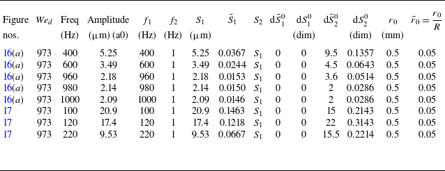
Finally, we compare the predictions with the experimental results of Dighe & Gadgil (Reference Dighe and Gadgil2019), for forcing applied through an acoustic source. Dighe & Gadgil (Reference Dighe and Gadgil2019) used Squire’s aerodynamic theory to calculate the cutoff frequency beyond which the sheet is stable to infinitesimal perturbations. Figure 16 shows the experimental growth curves for five different forcing frequencies, starting from 400 up to 1000 Hz. The predictions of the modified thinning theory agree only partially with the experimental growth. As seen in table 5 in Appendix A, the initial slope saturates at 980 Hz for
 $\textit{We}_{{d}} = 973$
, which is consistent with the authors’ observation identifying it as the cutoff frequency. Beyond the cutoff frequency, the initial growth is captured well by the theory (see figures 16(d) and 16(e)). However, the theory does not predict the overall growth at distances greater than approximately
 $r/d_{\!{j}}\gt 100$
. The predictions are consistent with experimental observations for frequencies well below the cutoff frequency (see figure 17). Here again, the theory predicts spatial growth close to the impingement point but deviates at larger distances.
Comparison of experimental sheet envelope with the thinning theory at
 $\textit{We}_{{d}} = 973$
near cutoff frequencies.

Comparison of experimental sheet envelope with the thinning theory at
 $\textit{We}_{{d}} = 973$
at frequencies lower than the cutoff value.

4. Conclusion
In this work, we show that a sinuous perturbation introduced at the centre of an expanding liquid sheet may grow spatially even in the absence of aerodynamic interactions. The growth occurs over a limited range of frequencies and for perturbations of finite slope at the impingement point. We hypothesise that the growth of sinuous perturbation introduced at the impingement point at a forcing frequency, and especially at low Weber numbers, may be attributed to disturbances caused by a combination of the displacements at the forcing frequency and that of the low-frequency noise. The source of the latter could be vibrations in the set-up or impact waves created at the point of impingement. For the perturbation to grow, the slope of the low noise disturbance needs to be finite but can be very small,
 $\mathcal{O}(0.1^{\circ }$
) or lower. The predictions of such a model agree well with the experimental observations for smooth and transition regimes. The main results of the study are summarised as follows.
-
(i) The modified thinning theory predicts instabilities to grow over a finite range of frequencies.
-
(ii) A combination of forcing frequency and a low-frequency noise with finite slope at the impingement point results in a sinuous growth that is close to those observed by Bremond et al. (Reference Bremond, Clanet and Villermaux2007) and Gyurkovich & Mehring (Reference Gyurkovich and Mehring2023) for Weber numbers up to 850. For higher Weber numbers, there are significant differences. Similarly, the predictions show better agreement for low Weber numbers compared with higher values for the experiments of Paramati et al. (Reference Paramati, Tirumkudulu and Schmid2015).
-
(iii) The phase velocity predicted by the normal mode analysis of the modified thinning model agrees closely with the measurement (Paramati et al. Reference Paramati, Tirumkudulu and Schmid2015). However, the phase velocity extracted from the solution of the full equations of the modified thinning model shows local variation in the phase velocity that is not observed in experiments.
-
(iv) There is only moderate agreement between the model predictions and the measured data for the case of Majumdar & Tirumkudulu (Reference Majumdar and Tirumkudulu2018).
-
(v) In the case of Dighe & Gadgil (Reference Dighe and Gadgil2019), the model predictions show moderate agreement with the measurements.
While these results are encouraging, there is a need to formulate a theory that accounts for both thinning of the liquid sheet and the aerodynamic interactions to capture the full dynamics over the entire range of Weber numbers. However, due to the presence of noise in the system, which can significantly influence the dynamics of the sheet, there will always remain a degree of uncertainty while comparing predictions of models with measurements.
Acknowledgements
S.K. acknowledges the Teaching Assistantship from IIT Bombay. The authors thank Prof E.J. Hinch for suggesting the compact derivation of equation (2.4).
Funding
M.S.T. acknowledges funding from the Abdul Kalam Technology Innovation National Fellowship and Department of Science and Technology (EMR/2017/001630).
Declaration of interests
The authors have no competing interests.
Appendix A. Parameters for the modified thinning model
In the modified thinning model discussed in this paper, several parameters have been used to obtain the model prediction. These include the frequency, slope and amplitude of the forced perturbation (
 $f_1, \text{d}\bar {S}_1^0, \bar {S}_1$
) and the low-frequency noise present (
 $f_2, \text{d}\bar {S}_2^0, \bar {S}_2$
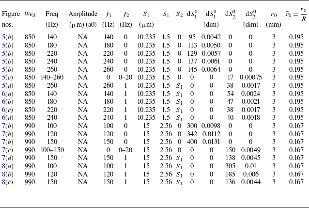
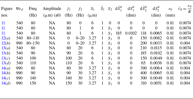
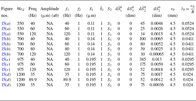
) in the system. Tables 1, 2, 3, 4 and 5 list the figure numbers and the corresponding experimental Weber numbers, frequencies and amplitudes in the first four columns for various figures. The remaining columns display the input parameters provided to the thinning model to fit the experimental results. Note that the perturbation slope (
 $\bar {S}_{\!j}^0$
) scales as
 $H/R$
. Both dimensional and non-dimensional values are provided since the characteristic length scales vary for various studies as well as the Weber numbers. The initial location
 $ r_0$
is defined as the point where the free liquid sheet begins to form,
 $ r_0 = d_{\!j}/2$
for the two-jet assembly and
 $ r_0 = d_i/2$
for the jet-impactor configuration, with a few exceptions made for comparisons with the experimental data of Gyurkovich & Mehring (Reference Gyurkovich and Mehring2023).
Input parameters to the thinning model used to fit theory with experiments of Gyurkovich & Mehring (Reference Gyurkovich and Mehring2023) (
 $\rho _{{l}} = 1000$
Kg m
 $^{-3}$
,
 $\sigma = 0.073$
Nm−1). Note that the value of
 $r_0$
, the initial point of perturbation, was adjusted so that the radial position of the first peak (antinode) in the experiments matches the prediction. In all other comparisons,
 $r_0$
is taken as the radius of the impactor (for impactor-jet configuation) or radius of the jet (for two-jet configuration).

Input parameters to the thinning model used to fit theory with experiments of Bremond et al. (Reference Bremond, Clanet and Villermaux2007) (
 $\rho _{{l}} = 1000$
Kg m
 $^{-3}$
,
 $\sigma = 0.073$
Nm−1).

Input parameters to the thinning model used to fit theory with experiments of Paramati et al. (Reference Paramati, Tirumkudulu and Schmid2015) (
 $\rho _{{l}} = 998$
Kg m
 $^{-3}$
,
 $\sigma = 0.072$
Nm−1).

Input parameters to the thinning model used to fit theory with experiments of Majumdar & Tirumkudulu (Reference Majumdar and Tirumkudulu2018) (
 $\rho _{{l}} = 998$
Kg m
 $^{-3}$
,
 $\sigma = 0.072$
Nm−1).

Input parameters to the thinning model used to fit theory with experiments of Dighe & Gadgil (Reference Dighe and Gadgil2019) (
 $\rho _{{l}} = 1205$
Kg m
 $^{-3}$
,
 $\sigma = 0.06487$
Nm−1).