1 Introduction
Droplet-based microfluidics has received extensive attention in the past decade owing to its great potential in scientific research and technical applications (Manga Reference Manga1996; Adamson et al. Reference Adamson, Mustafi, Zhang, Zheng and Ismagilov2006; Baroud, Gallaire & Dangla Reference Baroud, Gallaire and Dangla2010; Vladisavljević et al. Reference Vladisavljević, Khalid, Neves, Kuroiwa, Nakajima, Uemura, Ichikawa and Kobayashi2013). Two basic merits of droplet-based microfluidics, i.e. precise control of miniature droplet volumes and reliable manipulation of individual droplets, offer the feasibility of screening and analysing (bio)chemical reaction products (Song, Tice & Ismagilov Reference Song, Tice and Ismagilov2003; Zheng & Ismagilov Reference Zheng and Ismagilov2005), fabricating advanced materials (Zhao et al. Reference Zhao, Zhao, Hu, Xu, Zhao, Sun, Zhu, Xu and Gu2009; Shang et al. Reference Shang, Cheng, Wang, Yu, Zhao, Chen and Gu2016), etc. In applications of droplet-based microfluidics, a T-junction, a basic microfluidic passive-control element, is widely used for generating droplets (Thorsen et al. Reference Thorsen, Roberts, Arnold and Quake2001; De Menech et al. Reference De Menech, Garstecki, Jousse and Stone2008), for their merging (Christopher et al. Reference Christopher, Bergstein, End, Poon, Nguyen and Anna2009) and for their breakup (Link et al. Reference Link, Anna, Weitz and Stone2004; Jullien et al. Reference Jullien, Tsang Mui Ching, Cohen, Menetrier and Tabeling2009; Leshansky & Pismen Reference Leshansky and Pismen2009; Leshansky et al. Reference Leshansky, Afkhami, Jullien and Tabeling2012; Hoang et al. Reference Hoang, Portela, Kleijn, Kreutzer and van Steijn2013). In particular, droplet breakup in sequential T-junctions can produce small droplets in parallel (Link et al. Reference Link, Anna, Weitz and Stone2004; Adamson et al. Reference Adamson, Mustafi, Zhang, Zheng and Ismagilov2006; Abate & Weitz Reference Abate and Weitz2011), which provides a new route for mass production of microdroplets through microchannel networks. In this context, it is of great importance to fully understand the elementary process – the dynamic behaviour of droplets through a microfluidic T-junction.
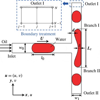
Schematic of droplet breakup in a T-junction (unless otherwise noted,
 $w_{0}=w_{1}=w$
).

Since Link et al. (Reference Link, Anna, Weitz and Stone2004) pioneered the introduction of T-junctions to passively split droplets into miniature sizes, considerable effort has been devoted to elucidating the mechanism of droplet breakup in a microfluidic T-junction. As reported by Jullien et al. (Reference Jullien, Tsang Mui Ching, Cohen, Menetrier and Tabeling2009), when droplets pass through a T-junction, there exist three distinct typical flow patterns, i.e., non-breakup, breakup with tunnels and breakup with permanent obstruction. It was found that the flow pattern of the passing droplet depends on the capillary number
 $Ca$
and the dimensionless initial droplet length
 $l_{0}/w$
, where
 $w$
is the channel width (see figure 1). To explore the underlying mechanisms, Leshansky & Pismen (Reference Leshansky and Pismen2009) and Leshansky et al. (Reference Leshansky, Afkhami, Jullien and Tabeling2012) theoretically and systematically investigated the processes of droplet breakup with tunnels and droplet breakup with a permanent obstruction by means of the lubrication analysis method, which theoretically analyses the breakup process by describing the behaviour of a lubricating film between the droplet and side walls at small capillary numbers. The results indicated that at moderate capillary numbers, the threshold between droplet flow patterns (breakup with tunnels and with permanent obstruction) can be predicted from
 $l_{0}/w=1.76(\unicode[STIX]{x1D6FC}/3Ca)^{1/3}+1$
with
 $\unicode[STIX]{x1D6FC}=0.25$
(Leshansky et al.
Reference Leshansky, Afkhami, Jullien and Tabeling2012), and the threshold between droplet breakup with tunnels and non-breakup is derived as
 $l_{0}/w=1.3Ca^{-0.21}$
(Leshansky & Pismen Reference Leshansky and Pismen2009), which has been validated in the experimental studies of Jullien et al. (Reference Jullien, Tsang Mui Ching, Cohen, Menetrier and Tabeling2009). In addition, the results indicated that the droplet breakup is driven chiefly by the buildup of pressure upstream (Leshansky & Pismen Reference Leshansky and Pismen2009). Later on, Hoang et al. (Reference Hoang, Portela, Kleijn, Kreutzer and van Steijn2013) developed a three dimensional numerical model to investigate the breakup process of sufficiently long droplets at a T-junction and found a critical neck thickness
 $\unicode[STIX]{x1D6FF}_{c}$
that determines whether the droplet pinch-off process is dominated by the continuous flow or surface tension. Besides these investigations of droplet breakup, a similar process, bubble breakup in a T-junction, has also drawn more attention in recent years (Fu et al.
Reference Fu, Ma, Funfschilling and Li2011; Fu & Ma Reference Fu and Ma2015; Wang et al.
Reference Wang, Zhu, Wu, Fu and Ma2015; Lu et al.
Reference Lu, Fu, Zhu, Ma and Li2016). As shown in their studies, there exists a distinct divergence of the breakup rate when bubbles are squeezed to pinch off, which is also observed in cases of droplet breakup (Jullien et al.
Reference Jullien, Tsang Mui Ching, Cohen, Menetrier and Tabeling2009; Hoang et al.
Reference Hoang, Portela, Kleijn, Kreutzer and van Steijn2013).
As mentioned above, considerable research has been devoted to revealing the breakup mechanisms in a T-junction. However, little attention is paid to the hydrodynamics underlying the non-breakup of a droplet. In fact, the mechanism behind droplet non-breakup has attracted increasing interest recently, due to its importance in droplet manipulation through microfluidics. Afkhami, Leshansky & Renardy (Reference Afkhami, Leshansky and Renardy2011) and Hoang (Reference Hoang2013) have found that under a symmetric boundary condition, non-breakup droplets finally attain a steady state, when vortex flows grow inside the droplet and continuous flow passes through the tunnels and gutters, exerting shear actions on the droplet. However, non-breakup processes have not been sufficiently discussed in their studies. In 1984, Rallison found that the vorticity in external flow highly inhibits droplet deformation (Rallison Reference Rallison1984). This suggests to us that vortex flows inside droplets might play an important role in the non-breakup of droplets through T-junctions, which has been little noticed previously. In addition, the real role of shear action induced by the effect of tunnels in a confined T-junction and the quantitative evolution of the competing forces involved are not completely elucidated, which are both the key points in a deep understanding of the non-breakup mechanisms. Moreover, the effects of the viscosity ratio between disperse and continuous phases and the width ratio between branch and main channels on droplet dynamic behaviours through the T-junction need further exploration.
Therefore, we employ here a phase-field multiphase lattice Boltzmann model to gain a deep understanding of the droplet non-breakup process in a microfluidic T-junction, while the detailed breakup hydrodynamics are also presented for comparison. The driving force behind and barriers to droplet deformation are analysed quantitatively and the temporal morphological characteristics of a deforming droplet are presented in detail. In order to further reveal the non-breakup mechanism, the roles of two hydrodynamic parameters – the shear stress and vorticity – are particularly examined and discussed. Furthermore, phase diagrams for the droplet dynamic behaviours through the T-junction are provided, based on which the effects of viscosity ratio between disperse and continuous phases and width ratio between branch and main channels are clarified.
2 Numerical method
2.1 Phase-field theory
The simulation of interfacial dynamics is a major challenge in multiphase flow modeling. The phase-field method, which is based on models of fluid free energy, has a firm foundation in interface physics. In this diffuse interface method, the thermodynamics of fluids is expressed by the free-energy functional of an order parameter
 $\unicode[STIX]{x1D719}$
, which distinguishes the different fluids. The free-energy function (Kendon et al.
Reference Kendon, Cates, Pagonabarraga, Desplat and Bladon2001) is defined as
 $$\begin{eqnarray}F=\int \left(\unicode[STIX]{x1D713}(\unicode[STIX]{x1D719})+\frac{1}{2}\unicode[STIX]{x1D705}|\unicode[STIX]{x1D735}\unicode[STIX]{x1D719}|^{2}+\unicode[STIX]{x1D70C}c_{s}^{2}\ln \unicode[STIX]{x1D70C}\right)\,\text{d}V,\end{eqnarray}$$
where
 $\unicode[STIX]{x1D70C}$
is the total density,
 $V$
denotes the fluid domain,
 $\unicode[STIX]{x1D713}(\unicode[STIX]{x1D719})$
is the bulk free-energy density, and the term
 $0.5\unicode[STIX]{x1D705}|\unicode[STIX]{x1D735}\unicode[STIX]{x1D719}|^{2}$
accounts for the interface energy with a positive coefficient
 $\unicode[STIX]{x1D705}$
. For a van der Waals fluid, the bulk free-energy density can be chosen as a double-well form (Kendon et al.
Reference Kendon, Cates, Pagonabarraga, Desplat and Bladon2001):
 $$\begin{eqnarray}\unicode[STIX]{x1D713}(\unicode[STIX]{x1D719})={\textstyle \frac{1}{4}}a(\unicode[STIX]{x1D719}-\unicode[STIX]{x1D719}_{A})^{2}(\unicode[STIX]{x1D719}-\unicode[STIX]{x1D719}_{B})^{2},\end{eqnarray}$$
where
 $a$
is a positive constant relating to the interfacial thickness
 $\unicode[STIX]{x1D709}$
and the surface tension
 $\unicode[STIX]{x1D70E}$
,
 $$\begin{eqnarray}\displaystyle & \displaystyle \unicode[STIX]{x1D709}=\frac{1}{|\unicode[STIX]{x1D719}_{A}-\unicode[STIX]{x1D719}_{B}|}\sqrt{\frac{8\unicode[STIX]{x1D705}}{a}}, & \displaystyle\end{eqnarray}$$
 $$\begin{eqnarray}\displaystyle & \displaystyle \unicode[STIX]{x1D70E}=\frac{|\unicode[STIX]{x1D719}_{A}-\unicode[STIX]{x1D719}_{B}|^{3}}{6}\sqrt{2\unicode[STIX]{x1D705}a}. & \displaystyle\end{eqnarray}$$
The subscripts
 $A$
and
 $B$
represent different fluids
 $A$
and
 $B$
in the two-phase flow system. Here, the chemical potential is derived as (Kendon et al.
Reference Kendon, Cates, Pagonabarraga, Desplat and Bladon2001)
 $$\begin{eqnarray}\unicode[STIX]{x1D707}=\frac{\unicode[STIX]{x1D6FF}F}{\unicode[STIX]{x1D6FF}\unicode[STIX]{x1D719}}=\unicode[STIX]{x1D713}^{\prime }(\unicode[STIX]{x1D719})-\unicode[STIX]{x1D705}\unicode[STIX]{x1D6FB}^{2}\unicode[STIX]{x1D719}=a(\unicode[STIX]{x1D719}-\unicode[STIX]{x1D719}_{A})(\unicode[STIX]{x1D719}-\unicode[STIX]{x1D719}_{B})\left(\unicode[STIX]{x1D719}-\frac{\unicode[STIX]{x1D719}_{a}+\unicode[STIX]{x1D719}_{B}}{2}\right)-\unicode[STIX]{x1D705}\unicode[STIX]{x1D6FB}^{2}\unicode[STIX]{x1D719}.\end{eqnarray}$$
As van der Waals hypothesized, the equilibrium interface profile is obtained by setting
 $\unicode[STIX]{x1D707}=0$
. And the one-dimensional solution of
 $\unicode[STIX]{x1D707}=0$
(along the
 $z$
direction) is given by
 $$\begin{eqnarray}\unicode[STIX]{x1D719}(z)=\frac{\unicode[STIX]{x1D719}_{A}+\unicode[STIX]{x1D719}_{B}}{2}+\frac{\unicode[STIX]{x1D719}_{A}-\unicode[STIX]{x1D719}_{B}}{2}\tanh \left(\frac{z}{\unicode[STIX]{x1D709}}\right).\end{eqnarray}$$
Based on van der Waals’s hypothesis, Cahn & Hilliard (Reference Cahn and Hilliard1958) derive the Cahn–Hilliard equation by assuming that the interfacial diffusion is driven by the chemical potential gradient, which is given by
 $$\begin{eqnarray}\frac{\unicode[STIX]{x2202}\unicode[STIX]{x1D719}}{\unicode[STIX]{x2202}t}+\unicode[STIX]{x1D735}\boldsymbol{\cdot }(\unicode[STIX]{x1D719}\boldsymbol{u})=M\unicode[STIX]{x1D6FB}^{2}\unicode[STIX]{x1D707},\end{eqnarray}$$
where
 $M$
is the mobility and
 $\boldsymbol{u}$
is the fluids’ velocity. The motion of the fluid is described by the Navier–Stokes equation (Jacqmin Reference Jacqmin1999)
 $$\begin{eqnarray}\displaystyle & \displaystyle \unicode[STIX]{x1D735}\boldsymbol{\cdot }\boldsymbol{u}=0, & \displaystyle\end{eqnarray}$$
 $$\begin{eqnarray}\displaystyle & \displaystyle \unicode[STIX]{x1D70C}\left(\frac{\unicode[STIX]{x2202}\boldsymbol{u}}{\unicode[STIX]{x2202}t}+\boldsymbol{u}\boldsymbol{\cdot }\unicode[STIX]{x1D735}\boldsymbol{u}\right)=-\unicode[STIX]{x1D735}p+\unicode[STIX]{x1D735}\boldsymbol{\cdot }[\unicode[STIX]{x1D702}(\unicode[STIX]{x1D735}\boldsymbol{u}+\unicode[STIX]{x1D735}\boldsymbol{u}^{\text{T}})]+\boldsymbol{F}_{s}, & \displaystyle\end{eqnarray}$$
where
 $\unicode[STIX]{x1D70C}$
is the total density of the fluids,
 $p$
is the hydrodynamic pressure,
 $\unicode[STIX]{x1D702}$
is the dynamic viscosity and
 $\boldsymbol{F}_{s}$
is the surface tension force, which is given by
 $\boldsymbol{F}_{s}=\unicode[STIX]{x1D707}\unicode[STIX]{x1D735}\unicode[STIX]{x1D719}$
(Jacqmin Reference Jacqmin1999; Liang et al.
Reference Liang, Shi, Guo and Chai2014).
2.2 The phase-field multiphase lattice Boltzmann model
In most lattice Boltzmann multiphase models (Gunstensen et al. Reference Gunstensen, Rothman, Zaleski and Zanetti1991; Shan & Chen Reference Shan and Chen1993, Reference Shan and Chen1994; Swift, Osborn & Yeomans Reference Swift, Osborn and Yeomans1995; Swift et al. Reference Swift, Orlandini, Osborn and Yeomans1996), the interface is tracked implicitly and the physics of the interface tracking equation is unknown. To describe interfacial dynamics explicitly, lattice Boltzmann multiphase models on the basis of the phase-field theory have been constructed and applied to dynamic multiphase flows (Liu & Zhang Reference Liu and Zhang2009; Liu, Zhang & Valocchi Reference Liu, Zhang and Valocchi2012; Liang et al. Reference Liang, Shi, Guo and Chai2014; Shi, Tang & Xia Reference Shi, Tang and Xia2014; Connington et al. Reference Connington, Miskin, Lee, Jaeger and Morris2015; Farokhirad, Morris & Lee Reference Farokhirad, Morris and Lee2015; Li et al. Reference Li, Luo, Kang, He, Chen and Liu2016; Liang, Shi & Chai Reference Liang, Shi and Chai2016). Here, we adopt the phase-field multiphase lattice Boltzmann model for a binary fluid proposed by Liu & Zhang (Reference Liu and Zhang2009) to study the breakup dynamics of a water droplet in a T-shaped junction filled with oil (see figure 1).
Note that the phase-field multiphase lattice Boltzmann model adopted here is two-dimensional. Compared with the three-dimensional model, the two-dimensional model omits two major issues in describing droplet behaviours through the T-junction, i.e. that continuous fluid passes over the droplet around the corners of the channel, and that there is a Laplace pressure due to the out-of-plane curvature on the droplet surface at the neck, which would accelerate the pinch-off of a droplet in a three-dimensional situation (Hoang Reference Hoang2013; Hoang et al.
Reference Hoang, Portela, Kleijn, Kreutzer and van Steijn2013). Actually, this problem has been proposed and discussed by Hoang et al. (Reference Hoang, Portela, Kleijn, Kreutzer and van Steijn2013). They found that a critical neck thickness,
 $\unicode[STIX]{x1D6FF}_{c^{\prime }}/w\approx h/(h+w)$
, triggers the onset of rapid collapse in a three-dimensional situation, which contributes to faster pinch-off of a droplet than in the two-dimensional situation. However, in the early stage of breakup when
 $\unicode[STIX]{x1D6FF}_{c^{\prime }}/w>h/(h+w)$
, the three-dimensional and two-dimensional evolutions of the dimensionless neck thickness are demonstrated to both follow the theoretical relation
 $\unicode[STIX]{x1D6FF}/w\approx 1-0.58(0.25/3Ca)^{-1/7}t^{3/7}$
(Leshansky et al.
Reference Leshansky, Afkhami, Jullien and Tabeling2012; Hoang et al.
Reference Hoang, Portela, Kleijn, Kreutzer and van Steijn2013). This indicates that, when
 $\unicode[STIX]{x1D6FF}_{c^{\prime }}/w>h/(h+w)$
, the three-dimensional effect at the neck (i.e. the Laplace pressure due to the out-of-plane curvature on the droplet surface at the neck) plays a negligible role in the droplet behaviours through the T-junction. Note that, in this paper, we focus on revealing the non-breakup mechanism of the droplet, when
 $\unicode[STIX]{x1D6FF}$
is generally larger than
 $\unicode[STIX]{x1D6FF}_{c^{\prime }}$
(Stone, Bentley & Leal Reference Stone, Bentley and Leal1986; Hoang Reference Hoang2013; Hoang et al.
Reference Hoang, Portela, Kleijn, Kreutzer and van Steijn2013). Therefore, the Laplace pressure due to the out-of-plane curvature in the three-dimensional situation is negligible here.
In addition to the three-dimensional effect at the neck, Hoang (Reference Hoang2013) has also made an effort to explore the influence of the flows around the corners in a three-dimensional channel. In his study, the continuous fluid was found to pass over a short non-breakup droplet via not only the tunnels (the lubricating film between the droplet and the channel walls) but also the gutters (the corners of the channel that are not filled by the droplet phase), which cannot be exactly described by the two-dimensional model. However, we also see that, although the two-dimensional model only represents the continuous fluid passing over a non-breakup droplet via the tunnels, the relevant two-dimensional theoretical predictions proposed by Leshansky & Pismen (Reference Leshansky and Pismen2009) and Leshansky et al. (Reference Leshansky, Afkhami, Jullien and Tabeling2012) agree well with the experimental data, especially the critical boundary data of droplet breakup and non-breakup. Therefore, the two-dimensional model indeed cannot exactly include all effects of continuous fluid passing over the droplet, which may result in inaccurate results such as a longer breakup time. However, it is capable of reflecting most hydrodynamics involved in the droplet behaviours through a T-junction, especially the non-breakup mechanism when
 $\unicode[STIX]{x1D6FF}_{c^{\prime }}/w>h/(h+w)$
.
The present model employs two distribution functions: the particle distribution function
 $f_{i}(\boldsymbol{x},t)$
and the order parameter distribution function
 $g_{i}(\boldsymbol{x},t)$
, which describe the evolution of the flow field and phase field, respectively. The evolution equations for
 $f_{i}$
and
 $g_{i}$
are (Liu & Zhang Reference Liu and Zhang2009)
 $$\begin{eqnarray}\displaystyle & \displaystyle f_{i}(\boldsymbol{x}+\boldsymbol{e}_{i}\unicode[STIX]{x1D6FF}_{t},t+\unicode[STIX]{x1D6FF}_{t})-f_{i}(\boldsymbol{x},t)=\frac{1}{\unicode[STIX]{x1D70F}_{f}}[f_{i}^{eq}(\boldsymbol{x},t)-f_{i}(\boldsymbol{x},t)]+F_{i}\unicode[STIX]{x1D6FF}_{t}, & \displaystyle\end{eqnarray}$$
 $$\begin{eqnarray}\displaystyle & \displaystyle g_{i}(\boldsymbol{x}+\boldsymbol{e}_{i}\unicode[STIX]{x1D6FF}_{t},t+\unicode[STIX]{x1D6FF}_{t})-g_{i}(\boldsymbol{x},t)=\frac{1}{\unicode[STIX]{x1D70F}_{g}}[g_{i}^{eq}(\boldsymbol{x},t)-g_{i}(\boldsymbol{x},t)], & \displaystyle\end{eqnarray}$$
where
 $\unicode[STIX]{x1D70F}_{f}$
and
 $\unicode[STIX]{x1D70F}_{g}$
are the relaxation parameters,
 $\unicode[STIX]{x1D6FF}_{t}$
is the lattice time step,
 $f_{i}^{eq}(\boldsymbol{x},t)$
and
 $g_{i}^{eq}(\boldsymbol{x},t)$
are the equilibrium distribution functions of
 $f_{i}$
and
 $g_{i}$
, and
 $F_{i}$
is the forcing term accounting for the interfacial force
 $\boldsymbol{F}_{s}$
in the lattice space.
The equilibrium distribution functions
 $f_{i}^{eq}(\boldsymbol{x},t)$
and
 $g_{i}^{eq}(\boldsymbol{x},t)$
and the forcing term
 $F_{i}$
can be written in power series in the particle velocity
 $\boldsymbol{u}$
(Liu & Zhang Reference Liu and Zhang2009),
 $$\begin{eqnarray}\displaystyle & \displaystyle f_{i}^{eq}=\unicode[STIX]{x1D714}_{i}\left[A_{i}+\unicode[STIX]{x1D70C}\left(\frac{\boldsymbol{e}_{i}\boldsymbol{\cdot }\boldsymbol{u}}{c_{s}^{2}}+\frac{(\boldsymbol{e}_{i}\boldsymbol{\cdot }\boldsymbol{u})^{2}}{2c_{s}^{4}}-\frac{\boldsymbol{u}^{2}}{2c_{s}^{2}}\right)\right], & \displaystyle\end{eqnarray}$$
 $$\begin{eqnarray}\displaystyle & \displaystyle g_{i}^{eq}=\unicode[STIX]{x1D714}_{i}\left[B_{i}+\unicode[STIX]{x1D719}\left(\frac{\boldsymbol{e}_{i}\boldsymbol{\cdot }\boldsymbol{u}}{c_{s}^{2}}+\frac{(\boldsymbol{e}_{i}\boldsymbol{\cdot }\boldsymbol{u})^{2}}{2c_{s}^{4}}-\frac{\boldsymbol{u}^{2}}{2c_{s}^{2}}\right)\right], & \displaystyle\end{eqnarray}$$
 $$\begin{eqnarray}\displaystyle & \displaystyle F_{i}=\left(1-\frac{1}{2\unicode[STIX]{x1D70F}_{f}}\right)\unicode[STIX]{x1D714}_{i}\left[\frac{(\boldsymbol{e}_{i}-\boldsymbol{u})}{c_{s}^{2}}+\frac{\boldsymbol{e}_{i}\boldsymbol{\cdot }\boldsymbol{u}}{c_{s}^{4}}\boldsymbol{e}_{i}\right]\boldsymbol{\cdot }\boldsymbol{F}_{s}, & \displaystyle\end{eqnarray}$$
where the factors
 $A_{i}$
and
 $B_{i}$
are given by
 $$\begin{eqnarray}\displaystyle & \displaystyle A_{i}=\left\{\begin{array}{@{}ll@{}}p/c_{s}^{2},\quad & i>0\\ \unicode[STIX]{x1D70C}-(1-\unicode[STIX]{x1D714}_{0})p/c_{s}^{2},\quad & i=0,\end{array}\right. & \displaystyle\end{eqnarray}$$
 $$\begin{eqnarray}\displaystyle & \displaystyle B_{i}=\left\{\begin{array}{@{}ll@{}}\unicode[STIX]{x1D6E4}\unicode[STIX]{x1D707}/c_{s}^{2},\quad & i>0\\ \hspace{0.0pt}[\unicode[STIX]{x1D719}-(1-\unicode[STIX]{x1D714}_{0})\unicode[STIX]{x1D6E4}\unicode[STIX]{x1D707}/c_{s}^{2}]/\unicode[STIX]{x1D714}_{0},\quad & i=0,\end{array}\right. & \displaystyle\end{eqnarray}$$
and
 $\unicode[STIX]{x1D6E4}$
is an adjustable parameter that controls the mobility. For the D2Q9 model, the weight factors
 $\unicode[STIX]{x1D714}_{i}$
and the discrete velocities
 $\boldsymbol{e}_{i}$
are defined by
 $$\begin{eqnarray}\displaystyle & \displaystyle \unicode[STIX]{x1D714}_{i}=\left\{\begin{array}{@{}ll@{}}4/9,\quad & i=0\\ 1/9,\quad & i=1,2,3,4\\ 1/36,\quad & i=5,6,7,8,\end{array}\right. & \displaystyle\end{eqnarray}$$
 $$\begin{eqnarray}\displaystyle & \displaystyle \boldsymbol{e}_{i}=\left\{\begin{array}{@{}ll@{}}0,\quad & i=0\\ c\{\cos [(i-1)\unicode[STIX]{x03C0}/2],\sin [(i-1)\unicode[STIX]{x03C0}/2]\},\quad & i=1,2,3,4\\ \sqrt{2}c\{\cos [(2i-9)\unicode[STIX]{x03C0}/4],\sin [(2i-9)\unicode[STIX]{x03C0}/4]\},\quad & i=5,6,7,8,\end{array}\right. & \displaystyle\end{eqnarray}$$
where
 $c=\unicode[STIX]{x1D6FF}_{x}/\unicode[STIX]{x1D6FF}_{t}$
is the lattice speed, in which
 $c=\sqrt{3}c_{s}$
,
 $c_{s}$
is the sound speed of the lattice fluid and
 $\unicode[STIX]{x1D6FF}_{x}$
is the lattice spacing.
In the present model, the macroscopic variables, such as the fluid density, velocity and pressure, and the order parameter are given by (Liu & Zhang Reference Liu and Zhang2009)
 $$\begin{eqnarray}\displaystyle & \displaystyle \unicode[STIX]{x1D70C}=\mathop{\sum }_{i=0}^{8}f_{i}, & \displaystyle\end{eqnarray}$$
 $$\begin{eqnarray}\displaystyle & \displaystyle \boldsymbol{u}=\frac{1}{\unicode[STIX]{x1D70C}}\left(\mathop{\sum }_{i=0}^{8}f_{i}\boldsymbol{e}_{i}+\frac{1}{2}\boldsymbol{F}_{s}\unicode[STIX]{x1D6FF}_{t}\right), & \displaystyle\end{eqnarray}$$
 $$\begin{eqnarray}\displaystyle & \displaystyle p=\unicode[STIX]{x1D70C}c_{s}^{2}+\unicode[STIX]{x1D707}\unicode[STIX]{x1D719}, & \displaystyle\end{eqnarray}$$
 $$\begin{eqnarray}\displaystyle & \displaystyle \unicode[STIX]{x1D719}=\mathop{\sum }_{i=0}^{8}g_{i}. & \displaystyle\end{eqnarray}$$
The Chapman–Enskog analysis on the evolution equations (2.10) and (2.11) indicates that the two lattice Boltzmann evolution equations can recover the Navier–Stokes equation and Cahn–Hilliard equation in the long-wavelength and low-frequency limit (Liu & Zhang Reference Liu and Zhang2009). The relationships between the macroscopic variables (dynamic viscosity
 $\unicode[STIX]{x1D702}$
and mobility
 $M$
) and the relaxation times are also derived as
 $$\begin{eqnarray}\displaystyle & \displaystyle \unicode[STIX]{x1D702}=\unicode[STIX]{x1D70C}c_{s}^{2}\unicode[STIX]{x1D6FF}_{t}\left(\unicode[STIX]{x1D70F}_{f}-{\textstyle \frac{1}{2}}\right), & \displaystyle\end{eqnarray}$$
 $$\begin{eqnarray}\displaystyle & \displaystyle M=\unicode[STIX]{x1D6E4}\unicode[STIX]{x1D6FF}_{t}\left(\unicode[STIX]{x1D70F}_{g}-{\textstyle \frac{1}{2}}\right), & \displaystyle\end{eqnarray}$$
where
 $\unicode[STIX]{x1D70F}_{g}=1/(3-\sqrt{3})$
to minimize the numerical errors of the convection–diffusion scheme (van der Sman Reference van der Sman2006). In the present model, the fluid is understood to be a mixture of oil and water components, where the dynamic viscosity of the binary fluid is defined as (Liu & Zhang Reference Liu and Zhang2009)
 $$\begin{eqnarray}\unicode[STIX]{x1D702}(\unicode[STIX]{x1D719})=\frac{1-\unicode[STIX]{x1D719}}{2}\unicode[STIX]{x1D702}_{o}+\frac{1+\unicode[STIX]{x1D719}}{2}\unicode[STIX]{x1D702}_{w},\end{eqnarray}$$
where
 $\unicode[STIX]{x1D702}_{o}$
and
 $\unicode[STIX]{x1D702}_{w}$
are the viscosities of the oil and water. The local relaxation time
 $\unicode[STIX]{x1D70F}_{f}$
can be calculated from the local viscosity
 $\unicode[STIX]{x1D702}(\unicode[STIX]{x1D719})$
. In order to keep the balance between the convection and diffusion effects at the interface, the interfacial thickness
 $\unicode[STIX]{x1D709}$
is set to 1.5 in this paper. In the framework of the lattice Boltzmann equation, the shear stress
 $\unicode[STIX]{x1D749}$
can be calculated from the non-equilibrium part of the distribution function (Chai & Zhao Reference Chai and Zhao2012)
 $$\begin{eqnarray}\unicode[STIX]{x1D749}=-\frac{2-1/\unicode[STIX]{x1D70F}_{f}}{4}\left(\unicode[STIX]{x1D6FF}_{t}(\boldsymbol{u}\boldsymbol{F}+\boldsymbol{F}\boldsymbol{u})+2\mathop{\sum }_{i}\boldsymbol{e}_{i}\boldsymbol{e}_{i}\,f_{i}^{neq}\right),\end{eqnarray}$$
where
 $f_{i}^{neq}$
is the local non-equilibrium part of the distribution function satisfying
 $f_{i}^{neq}=f_{i}-f_{i}^{eq}$
.
2.3 Boundary conditions
Boundary conditions are one of the key issues in lattice Boltzmann simulation. In a typical simulation of droplet breakup in a T-shaped junction, two kinds of boundary conditions are involved: the velocity boundary conditions at the inlet, outlet and solid walls of the channels and the wetting boundary condition for considering the fluid–solid interaction.
In this paper, the halfway bounce-back boundary scheme (Ladd Reference Ladd1994) is utilized at the inlet and solid walls of the channels. The unknown distribution functions at the inlet boundary are given by
 $$\begin{eqnarray}\displaystyle & \displaystyle f_{i^{\prime }}(\boldsymbol{x}_{in},t+\unicode[STIX]{x1D6FF}_{t})=f_{i}^{+}(\boldsymbol{x}_{in},t)-2\unicode[STIX]{x1D714}_{i}\unicode[STIX]{x1D70C}(\boldsymbol{x}_{in},t)\frac{\boldsymbol{e}_{i}\boldsymbol{\cdot }\boldsymbol{u}_{in}}{c_{s}^{2}}, & \displaystyle\end{eqnarray}$$
 $$\begin{eqnarray}\displaystyle & \displaystyle g_{i^{\prime }}(\boldsymbol{x}_{in},t+\unicode[STIX]{x1D6FF}_{t})=g_{i}^{+}(\boldsymbol{x}_{in},t)-2\unicode[STIX]{x1D714}_{i}\unicode[STIX]{x1D719}(\boldsymbol{x}_{in},t)\frac{\boldsymbol{e}_{i}\boldsymbol{\cdot }\boldsymbol{u}_{in}}{c_{s}^{2}}, & \displaystyle\end{eqnarray}$$
where
 $\boldsymbol{e}_{i^{\prime }}$
is the opposite velocity of
 $\boldsymbol{e}_{i}$
(
 $\boldsymbol{e}_{i^{\prime }}=-\boldsymbol{e}_{i}$
), and
 $\boldsymbol{u}_{in}$
is the velocity at the inlet boundary. In addition,
 $f_{i}^{+}$
and
 $g_{i}^{+}$
are the postcollision distribution functions,
 $$\begin{eqnarray}\displaystyle & \displaystyle f_{i}^{+}(\boldsymbol{x}_{in},t)=f_{i}(\boldsymbol{x}_{in},t)+\frac{1}{\unicode[STIX]{x1D70F}_{f}}[f_{i}^{eq}(\boldsymbol{x}_{in},t)-f_{i}(\boldsymbol{x}_{in},t)]+F_{i}\unicode[STIX]{x1D6FF}_{t}, & \displaystyle\end{eqnarray}$$
 $$\begin{eqnarray}\displaystyle & \displaystyle g_{i}^{+}(\boldsymbol{x}_{in},t)=g_{i}(\boldsymbol{x}_{in},t)+\frac{1}{\unicode[STIX]{x1D70F}_{g}}[g_{i}^{eq}(\boldsymbol{x}_{in},t)-g_{i}(\boldsymbol{x}_{in},t)]. & \displaystyle\end{eqnarray}$$
Similarly, the no-slip boundary condition at the solid walls is realized by
 $$\begin{eqnarray}\displaystyle & \displaystyle f_{i^{\prime }}(\boldsymbol{x}_{wall},t+\unicode[STIX]{x1D6FF}_{t})=f_{i}^{+}(\boldsymbol{x}_{wall},t), & \displaystyle\end{eqnarray}$$
 $$\begin{eqnarray}\displaystyle & \displaystyle g_{i^{\prime }}(\boldsymbol{x}_{wall},t+\unicode[STIX]{x1D6FF}_{t})=g_{i}^{+}(\boldsymbol{x}_{wall},t). & \displaystyle\end{eqnarray}$$
The convective outflow boundary condition is adopted at the outlets in this paper for its good performance at the open boundary of the multiphase flow (Lou, Guo & Shi Reference Lou, Guo and Shi2013). The unknown distribution functions at outlet I (see figure 1) are given by
 $$\begin{eqnarray}\displaystyle & \displaystyle f_{i}(j,N,t+\unicode[STIX]{x1D6FF}_{t})=\frac{f_{i}(j,N,t)+\unicode[STIX]{x1D6EC}f_{i}(j,N-1,t+\unicode[STIX]{x1D6FF}_{t})}{1+\unicode[STIX]{x1D6EC}}, & \displaystyle\end{eqnarray}$$
 $$\begin{eqnarray}\displaystyle & \displaystyle g_{i}(j,N,t+\unicode[STIX]{x1D6FF}_{t})=\frac{g_{i}(j,N,t)+\unicode[STIX]{x1D6EC}g_{i}(j,N-1,t+\unicode[STIX]{x1D6FF}_{t})}{1+\unicode[STIX]{x1D6EC}}, & \displaystyle\end{eqnarray}$$
where
 $\unicode[STIX]{x1D6EC}=U_{ave}(t+\unicode[STIX]{x1D6FF}_{t})\unicode[STIX]{x1D6FF}_{t}/\unicode[STIX]{x1D6FF}_{y}$
, and
 $U_{ave}(t+\unicode[STIX]{x1D6FF}_{t})$
is a typical velocity normal to the outlet boundary (Lou et al.
Reference Lou, Guo and Shi2013). In this work,
 $$\begin{eqnarray}U_{ave}(t+\unicode[STIX]{x1D6FF}_{t})=\frac{1}{\text{No.}+1}\mathop{\sum }_{j}v(j,N-1,t+\unicode[STIX]{x1D6FF}_{t}),\end{eqnarray}$$
where
 $0\leqslant j\leqslant \text{No.}$
and
 $\text{No.}+1$
is the number of nodes in the (
 $N-1$
)th layer in the
 $x$
direction. The microscopic variables can also be derived as
 $$\begin{eqnarray}\unicode[STIX]{x1D712}(j,N,t+\unicode[STIX]{x1D6FF}_{t})=\frac{\unicode[STIX]{x1D712}(j,N,t)+\unicode[STIX]{x1D6EC}\unicode[STIX]{x1D712}(j,N-1,t+\unicode[STIX]{x1D6FF}_{t})}{1+\unicode[STIX]{x1D6EC}},\end{eqnarray}$$
where
 $\unicode[STIX]{x1D712}$
can be the density, pressure or order parameter of the fluid. The boundary treatment at outlet II is realized similarly.
To describe the fluid–solid interaction, the wetting boundary condition proposed by van der Graaf et al. (Reference van der Graaf, Nisisako, Schroen, van der Sman and Boom2006) is adopted in this work. They assume that the wall is a mixture of the two fluids with the order parameter
 $\unicode[STIX]{x1D719}_{wall}$
, and the relations of the interfacial tensions of the fluids with solid walls are also given by (Liu & Zhang Reference Liu and Zhang2009)
 $$\begin{eqnarray}\displaystyle & \displaystyle \unicode[STIX]{x1D70E}_{o,wall}=\frac{\unicode[STIX]{x1D705}\unicode[STIX]{x1D719}_{oil}^{2}}{\unicode[STIX]{x1D709}}\left\{\frac{2}{3}-\left[\frac{\unicode[STIX]{x1D719}_{wall}}{\unicode[STIX]{x1D719}_{oil}}-\frac{1}{3}\left(\frac{\unicode[STIX]{x1D719}_{wall}}{\unicode[STIX]{x1D719}_{oil}}\right)^{3}\right]\right\}, & \displaystyle\end{eqnarray}$$
 $$\begin{eqnarray}\displaystyle & \displaystyle \unicode[STIX]{x1D70E}_{w,wall}=\frac{\unicode[STIX]{x1D705}\unicode[STIX]{x1D719}_{water}^{2}}{\unicode[STIX]{x1D709}}\left\{\frac{2}{3}-\left[\frac{\unicode[STIX]{x1D719}_{wall}}{\unicode[STIX]{x1D719}_{water}}-\frac{1}{3}\left(\frac{\unicode[STIX]{x1D719}_{wall}}{\unicode[STIX]{x1D719}_{water}}\right)^{3}\right]\right\}, & \displaystyle\end{eqnarray}$$
where
 $\unicode[STIX]{x1D70E}_{o,wall}$
is the interfacial tension of oil with solid wall,
 $\unicode[STIX]{x1D70E}_{w,wall}$
is the interfacial tension of water with solid wall,
 $\unicode[STIX]{x1D719}_{oil}=-1$
and
 $\unicode[STIX]{x1D719}_{water}=+1$
in this paper.
According to Young’s law, the contact angle is given by
 $$\begin{eqnarray}\cos (\unicode[STIX]{x1D703})=\frac{\unicode[STIX]{x1D70E}_{w,wall}-\unicode[STIX]{x1D70E}_{o,wall}}{\unicode[STIX]{x1D70E}_{ow}}.\end{eqnarray}$$
Substituting (2.4), (2.37) and (2.38) into (2.39), we can derive the relation between the contact angle and the order parameter of the solid wall:
 $$\begin{eqnarray}\cos (\unicode[STIX]{x1D703})={\textstyle \frac{1}{2}}\unicode[STIX]{x1D719}_{wall}(3-\unicode[STIX]{x1D719}_{wall}^{2}).\end{eqnarray}$$
The validation of the contact angle is given in § 3. For details of the wetting boundary condition, refer to the work of van der Graaf et al. (Reference van der Graaf, Nisisako, Schroen, van der Sman and Boom2006).
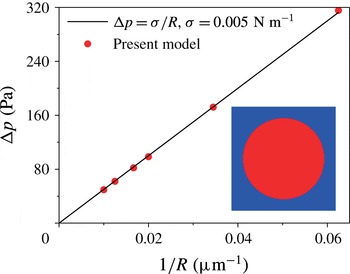
Numerical validation of Laplace’s law.

3 Case validation
In this section, several numerical examples are employed to validate the present phase-field multiphase lattice Boltzmann model. For the first benchmark case, we consider a static circular water droplet located at the center of a
 $256~\unicode[STIX]{x03BC}\text{m}\times 256~\unicode[STIX]{x03BC}\text{ m}$
domain filled with oil. Periodic boundary conditions are applied to all boundaries. In this simulation, the corresponding physical values of the water and oil are given by
 $\unicode[STIX]{x1D70C}_{w}=\unicode[STIX]{x1D70C}_{o}=1000~\text{ kg}~\text{m}^{-3}$
,
 $\unicode[STIX]{x1D702}_{o}=8\unicode[STIX]{x1D702}_{w}=0.008~\text{ Pa}~\text{ s}$
and
 $\unicode[STIX]{x1D70E}=0.005~\text{ N}~\text{ m}^{-1}$
. The lattice spacing
 $\unicode[STIX]{x1D6FF}_{x}$
equals
 $1~\unicode[STIX]{x03BC}\text{m}$
in physical units. Some other parameters are adopted as follows:
 $\unicode[STIX]{x1D70F}_{g}=1/(3-\sqrt{3})$
,
 $\unicode[STIX]{x1D709}=1.5\unicode[STIX]{x1D6FF}_{x}$
and
 $\unicode[STIX]{x1D6E4}=4.0$
. In the equilibrium state, the pressure difference
 $\unicode[STIX]{x0394}p$
sustained across the droplet interface can be calculated according to Laplace’s law,
 $$\begin{eqnarray}\unicode[STIX]{x0394}p=\frac{\unicode[STIX]{x1D70E}}{R},\end{eqnarray}$$
where
 $R$
is the droplet radius. As seen in figure 2, the numerical results of the present model are in good agreement with the analytical solution of (3.1), which demonstrates that the present model is capable of predicting the correct surface tension.
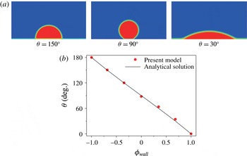
The above test does not involve the interaction between liquids and the solid wall. To verify the wetting boundary condition adopted here, we simulate the contact angles of droplets on the solid surface. At the beginning, a circular water droplet of radius
 $R=20~\unicode[STIX]{x03BC}\text{m}$
is deposited on the solid bottom surface. The computational domain is
 $150~\unicode[STIX]{x03BC}\text{m}\times 150~\unicode[STIX]{x03BC}\text{m}$
and full of oil except for the droplet region. The halfway bounce-back boundary scheme and wetting boundary condition are utilized for the solid walls and the theoretical contact angle is given by (2.40). For uniformity, the parameters of the liquids are as same as in the above case. We conduct the simulations until the droplet reaches an equilibrium state. The results with the static contact angles
 $\unicode[STIX]{x1D703}=30^{\circ },90^{\circ }$
and
 $150^{\circ }$
are shown in figure 3(a), and figure 3(b) presents the linear relationship between contact angle and the order parameter of the solid wall. As shown, the numerical results agree well with the analytical solution of (2.40). This confirms the suitability of the current wetting boundary condition.
Numerical validation of contact angle: (a) droplet contours of different contact angles, (b) the linear relationship between contact angle and the order parameter of a solid wall.

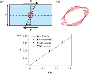
Ensuring that the present model is suited for the static situation, we now further validate the model with a dynamic problem – Taylor deformation – involving large changes of the interface. In this problem, a droplet is deforming under a linear shear flow (see figure 4 a) in the Stokes regime. The droplet deformation has been extensively investigated as a function of the shear rate (expressed as the capillary number) (Roths et al. Reference Roths, Friedrich, Marth and Honerkamp2002). The Reynolds number and capillary number are defined as
 $$\begin{eqnarray}\displaystyle & \displaystyle Re=\frac{\unicode[STIX]{x1D6FE}R^{2}\unicode[STIX]{x1D70C}}{\unicode[STIX]{x1D702}}, & \displaystyle\end{eqnarray}$$
 $$\begin{eqnarray}\displaystyle & \displaystyle Ca=\frac{\unicode[STIX]{x1D6FE}R\unicode[STIX]{x1D702}}{\unicode[STIX]{x1D70E}}, & \displaystyle\end{eqnarray}$$
where
 $\unicode[STIX]{x1D6FE}$
is the shear rate and
 $R$
is the initial radius of the droplet. Just as in the first two validation cases, the same physical parameters are adopted, except that
 $\unicode[STIX]{x1D702}_{o}=\unicode[STIX]{x1D702}_{w}=0.001~\text{Pa}~\text{s}$
. All simulations are run under the uniform grid mesh of
 $256\times 128$
cells at
 $Re=0.1$
. When the droplet deformation stabilizes, the droplet has an elliptic shape, which is usually characterized by the Taylor deformation parameter
 $D$
, given by
 $$\begin{eqnarray}D=\frac{L-B}{L+B},\end{eqnarray}$$
where
 $L$
and
 $B$
are the ellipse’s major and minor axes, respectively. Figure 4(b) shows the elliptic interface profiles of the steady deformed droplets for several capillary numbers. As seen in the figure, the deformation becomes more serious with increasing capillary number and all profiles cross two points consistent with other works (Zhou & Pozrikidis Reference Zhou and Pozrikidis1993; Liu & Zhang Reference Liu and Zhang2011; Shi et al.
Reference Shi, Tang and Xia2014). The relationship between
 $D$
and
 $Ca$
is presented in figure 4(c), where the numerical results of the present model agree well with those of the VOF method and Swift’s model (Liu Reference Liu2010). Based on the present numerical results, a linear relationship between
 $D$
and
 $Ca$
is also given:
 $D=1.44Ca$
. These analyses indicate that the large interface deformation can be simulated fairly well by the present model.
Numerical validation of Taylor deformation: (a) schematic of the initial configuration and location of the droplet in shear flow, (b) steady droplet shapes depicted as contour lines of
 $\unicode[STIX]{x1D719}=0$
for several capillary numbers
 $Ca=0.05,0.1,0.15,0.2,0.25,0.3$
and (c) relationship between capillary number and Taylor deformation parameter.

4 Results and discussion
By using the above validated method, a two-dimensional model of two-phase flow is developed to investigate the non-breakup and breakup dynamics of droplets in a microfluidic T-junction within the hydrodynamic regime where capillary forces and viscous stresses are dominant over inertia. As seen from figure 1, a water droplet with an initial length
 $l_{0}$
flows from the main channel of width
 $w_{0}$
into a T-junction with two equal arms of the same width
 $w_{1}$
. Unless otherwise noted, the widths of main and branch channels are both equal to
 $30~\unicode[STIX]{x03BC}\text{m}$
(i.e.
 $w_{0}=w_{1}=w=30~\unicode[STIX]{x03BC}\text{m}$
). The droplet is surrounded by the outer continuous oil, which carries the droplet with average velocity
 $U$
. The fluid properties adopted here include
 $\unicode[STIX]{x1D70C}_{w}=\unicode[STIX]{x1D70C}_{o}=1000~\text{kg}~\text{m}^{-3}$
,
 $\unicode[STIX]{x1D702}_{w}=0.001~\text{Pa}~\text{s}$
,
 $\unicode[STIX]{x1D702}_{o}=0.008~\text{Pa}~\text{s}$
,
 $\unicode[STIX]{x1D70E}=0.005~\text{N}~\text{m}^{-1}$
and the viscosity ratio
 $\unicode[STIX]{x1D706}=\unicode[STIX]{x1D702}_{w}/\unicode[STIX]{x1D702}_{o}=1/8$
(Link et al.
Reference Link, Anna, Weitz and Stone2004; Jullien et al.
Reference Jullien, Tsang Mui Ching, Cohen, Menetrier and Tabeling2009). In this study, the capillary number
 $Ca=\unicode[STIX]{x1D702}_{o}U/\unicode[STIX]{x1D70E}$
and Reynolds number
 $Re=\unicode[STIX]{x1D70C}_{o}Uw/\unicode[STIX]{x1D702}_{o}$
are in the ranges
 $5\times 10^{-3}<Ca<10^{-1}$
and
 $1.2\times 10^{-2}<Re<2.5\times 10^{-1}$
, respectively. The key parameters of the model are adopted as follows:
 $\unicode[STIX]{x1D70F}_{g}=1/(3-\sqrt{3})$
,
 $\unicode[STIX]{x1D709}=1.5\unicode[STIX]{x1D6FF}_{x}$
and
 $\unicode[STIX]{x1D6E4}=4.0$
.
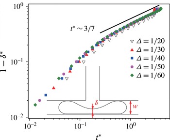
A grid independence test has also been conducted with five different mesh sizes,
 $\unicode[STIX]{x1D6E5}=\unicode[STIX]{x1D6FF}_{x}/w=1/20,1/30,1/40,1/50$
and
 $1/60$
, the results of which are depicted in figure 5 in terms of the temporal evolution of dimensionless neck thickness
 $\unicode[STIX]{x1D6FF}^{\ast }$
(
 $\unicode[STIX]{x1D6FF}^{\ast }=\unicode[STIX]{x1D6FF}/w$
) versus dimensionless time
 $t^{\ast }$
(
 $t^{\ast }=Ut/w$
). As seen in the figure, the numerical results become independent of mesh size when
 $\unicode[STIX]{x1D6E5}<1/20$
, which can be well described by the analytical
 $3/7$
scaling law (Leshansky et al.
Reference Leshansky, Afkhami, Jullien and Tabeling2012). Considering the tradeoff between model performance and computational requirements, we choose the grid mesh
 $\unicode[STIX]{x1D6E5}=1/30$
in the following simulations.
Evolution of the neck thickness for different grid resolutions (
 $\unicode[STIX]{x1D706}=1/8$
,
 $l_{0}/w=5.5$
,
 $Ca=1\times 10^{-2}$
).

4.1 Droplet dynamic behaviours in the microfluidic T-junction
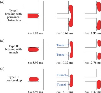
As reported by the previous study (Jullien et al. Reference Jullien, Tsang Mui Ching, Cohen, Menetrier and Tabeling2009), three distinct typical flow patterns of droplets through the T-junction are also successfully reproduced by the present numerical simulation, i.e., type I breakup with permanent obstruction, type II breakup with tunnels and type III non-breakup (see figure 6). It is worth noting that the distinction between types I and II is whether there are visible tunnels between droplets and walls (see figure 6 a,b). Although this purely geometrical classification ignores the cross-sectional geometries of droplets, it has been proved to be reasonable and has been widely adopted to study the process of droplet breakup in the microfluidic T-junction (Leshansky & Pismen Reference Leshansky and Pismen2009; Leshansky et al. Reference Leshansky, Afkhami, Jullien and Tabeling2012; Hoang et al. Reference Hoang, Portela, Kleijn, Kreutzer and van Steijn2013). Significantly, via detailed analysis of the hydrodynamic information involved in these flow patterns, we provide herein a deeper insight than previous studies into the effect of temporal competition between driving force and resistance on the dynamic behaviours through the T-junction. In particular, we offer a new vision to facilitate the understanding of the droplet non-breakup mechanism.
Three types of droplet behaviours in microfluidic T-junctions; the droplets move from left to right along the horizontal channel (
 $\unicode[STIX]{x1D706}=1/8$
,
 $Ca=0.05$
): (a) breakup with permanent obstruction (
 $l_{0}/w=3.73$
), (b) breakup with tunnels (
 $l_{0}/w=2.33$
), (c) non-breakup (
 $l_{0}/w=2.13$
).

4.1.1 Breakup with permanent obstruction
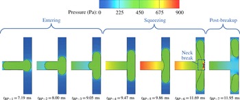
Evolution of the pressure field during droplet breakup with permanent obstruction in a T-junction (
 $\unicode[STIX]{x1D706}=1/8$
,
 $Ca=0.05$
,
 $l_{0}/w=3.73$
).

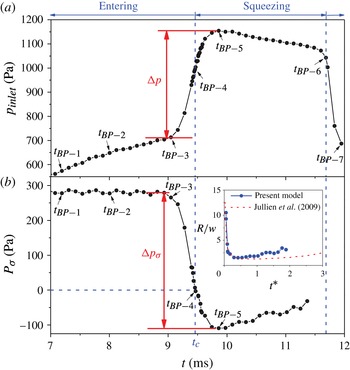
Generally, the buildup of upstream pressure and the surface tension of the droplet are correspondingly regarded as the main driving force and the resistance to droplet breakup through a microfluidic T-junction (Jullien et al.
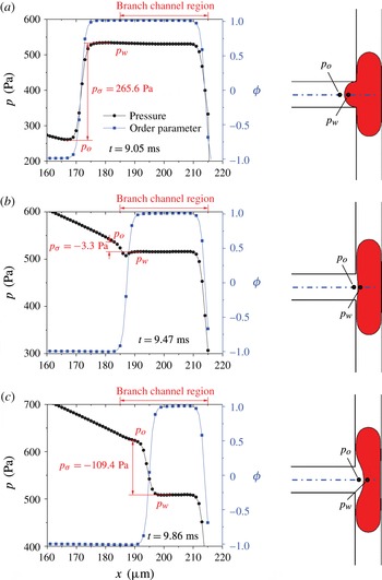
Reference Jullien, Tsang Mui Ching, Cohen, Menetrier and Tabeling2009; Leshansky & Pismen Reference Leshansky and Pismen2009). Accordingly, in order to clearly understand the competition between these two factors, figures 7–9 provide the detailed evolutions of the pressure distribution and the Laplace pressure drop across the rear droplet interface during the droplet breakup with permanent obstruction. As shown, based on the variation of the morphological characteristics of droplets, the process of breakup can be simply divided into three stages: entering, squeezing and post-breakup. More importantly, the pressure field exhibits characteristics corresponding to the droplet morphologies in these three stages. The order parameter distribution in figure 8 helps to identify the rear interface between
 $\unicode[STIX]{x1D719}=-1$
and
 $\unicode[STIX]{x1D719}=1$
. Accordingly, the pressure difference across the interface, i.e. the Laplace pressure
 $p_{\unicode[STIX]{x1D70E}}$
, can be obtained as
 $p_{\unicode[STIX]{x1D70E}}=p_{inside}-p_{outside}=p_{w}-p_{o}$
.
The pressure and order parameter distributions along the symmetry axis of the T-junction around the interface;
 $p_{\unicode[STIX]{x1D70E}}$
is the Laplace pressure across the interface given by
 $p_{\unicode[STIX]{x1D70E}}=p_{w}-p_{o}$
and negative values signify that the surface tension is oriented upstream (
 $\unicode[STIX]{x1D706}=1/8$
,
 $Ca=0.05$
,
 $l_{0}/w=3.73$
): (a)
 $t=9.05$
ms, (b)
 $t=9.47$
ms and (c)
 $t=9.86$
ms.

Evolution of the pressure for droplet breakup with permanent obstruction (
 $\unicode[STIX]{x1D706}=1/8$
,
 $Ca=0.05$
,
 $l_{0}/w=3.73$
): (a) the inlet pressure of the main channel, (b) the Laplace pressure of the rear droplet interface (negative values signify that the surface tension is oriented upstream). Inset: evolution of the curvature radius of the rear droplet interface at the squeezing stage,
 $t^{\ast }=(t-t_{c})U/w$
.

Upon arriving at the T-junction, the droplet first experiences the entering stage (see figure 7, entering stage). Initially, the droplet is deformed symmetrically with two identical ‘fingers’ obstructed into two branch channels and a rear one left in the main channel (before
 $t_{BP-3}=9.05$
ms in figure 7). In particular, the rear remains convex with a fixed shape (see
 $t_{BP-1}$
–
 $t_{BP-3}$
in figure 7), and thus the Laplace pressure across the rear interface,
 $p_{\unicode[STIX]{x1D70E}}$
, is unchanged during this stage (before
 $t_{BP-3}=9.05$
ms in figures 8 and 9). Furthermore, the inlet pressure of the T-junction,
 $p_{inlet}$
, climbs slowly to overcome the increasing resistance of capillary hysteresis owing to the decreasing advancing contact angle of two ‘fingers’. After the initial entering stage has ended at
 $t_{BP-3}=9.05$
ms, the rear interface of the droplet starts to be flattened by the accumulated pressure upstream, when
 $p_{inlet}$
begins to rise drastically (see
 $t_{BP-3}$
–
 $t_{BP-4}$
in figure 9
a). Corresponding to the changing curvature radius of the rear interface,
 $p_{\unicode[STIX]{x1D70E}}$
drops rapidly as shown in figure 9(b).
As shown in figure 7, when the rear is fully flattened at
 $t_{BP-4}=9.47$
ms (i.e. the critical time
 $t_{c}$
as
 $p_{\unicode[STIX]{x1D70E}}$
= 0 Pa in figure 9
b), the droplet entirely leaves the main channel and enters the squeezing stage. Then, the flat rear interface becomes concave and a neck is formed in the central position of the junction; this gradually thins out until breakup happens. During the entire squeezing stage, the interface tension of the rear is oriented upstream, and thus
 $p_{\unicode[STIX]{x1D70E}}$
maintains a negative value, as depicted in figure 8. Notably, in the initial period of the squeezing stage,
 $p_{inlet}$
continues to increase drastically, driving the increasing concavity of the rear (see
 $t_{BP-4}$
–
 $t_{BP-5}$
in figure 9
a). After that, with the continuing shrinkage and elongation of the neck, the curvature radius of the rear gradually increases, which reduces the absolute value of
 $p_{\unicode[STIX]{x1D70E}}$
. Meanwhile,
 $p_{inlet}$
experiences a proportional decrease (see
 $t_{BP-4}$
–
 $t_{BP-5}$
in figure 9). Such a correspondence between
 $p_{inlet}$
and
 $p_{\unicode[STIX]{x1D70E}}$
suggests that the buildup of upstream pressure is mainly devoted to overcoming the deformation resistance by interface tension of the rear. At the end of the squeezing stage, the droplet breaks up, producing two daughter droplets that move downstream (see post-breakup stage in figure 7). Meanwhile, the upstream pressure returns to normal immediately (see figure 9
a). Herein, the evolution of the curvature radius of the rear in the squeezing stage is also shown in the inset of figure 9(b), where the current results agree well with those of Jullien et al. (Reference Jullien, Tsang Mui Ching, Cohen, Menetrier and Tabeling2009). This further verifies the correctness of present model.
Evolution of the dimensionless characteristic parameters in the squeezing stage (
 $t^{\ast }=(t-t_{c})U/w$
,
 $\unicode[STIX]{x1D706}=1/8$
,
 $Ca=0.05$
,
 $l_{0}/w=3.73$
): (a) the neck thickness, inset: the same data as
 $\log (1-\unicode[STIX]{x1D6FF}^{\ast })$
versus
 $\log (t^{\ast })$
; (b) the distance travelled by the tip of the droplet; (c) the thickness of the film sandwiched between droplet and channel walls.

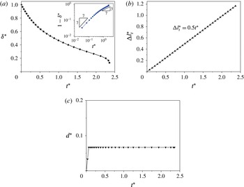
Toget adeeper understandingof thedroplet breakupmechanism,three dimensionless geometrical parameters are utilized to quantify the evolution of morphological characteristics during the squeezing stage (Jullien et al.
Reference Jullien, Tsang Mui Ching, Cohen, Menetrier and Tabeling2009; Wang et al.
Reference Wang, Zhu, Wu, Fu and Ma2015) (see figure 10), i.e. the neck thickness
 $\unicode[STIX]{x1D6FF}^{\ast }=\unicode[STIX]{x1D6FF}/w$
, the distance travelled by the tip of the droplet
 $\unicode[STIX]{x0394}l_{t}^{\ast }=(l_{t}-l_{0})/2w$
and the thickness of the film sandwiched between droplet and channel walls
 $d^{\ast }=d/w$
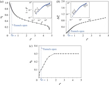
. As shown in figure 10(a), the neck thickness decreases monotonically until the breakup occurs. For a better understanding, the inset gives a log–log plot for the distance travelled by the rear of the droplet,
 $1-\unicode[STIX]{x1D6FF}^{\ast }$
versus
 $t^{\ast }$
. According to the exponent of the scaling law, there are two different substages in the squeezing stage. In the first substage,
 $1-\unicode[STIX]{x1D6FF}^{\ast }$
has a linear relationship with time
 $t^{\ast }$
, while it presents an exponential relationship,
 $1-\unicode[STIX]{x1D6FF}^{\ast }\sim t^{\ast ~3/7}$
, in the second stage, where the
 $3/7$
scaling agrees well with the theoretical solution (Leshansky et al.
Reference Leshansky, Afkhami, Jullien and Tabeling2012; Hoang et al.
Reference Hoang, Portela, Kleijn, Kreutzer and van Steijn2013). Such a temporal variation of neck thickness can also be attributed to the governing forces involved. In the first substage, the surface tension is too small due to little deformation of the rear of the droplet. Therefore, due to inertia, the rear interface keeps moving with the original velocity
 $U$
with little resistance from the surface tension, which leads to a linear relationship between
 $1-\unicode[STIX]{x1D6FF}^{\ast }$
and
 $t^{\ast }$
. The duration of the first substage is very short because of the rapid increase in surface tension at the rear. Subsequently it transitions to the second substage with an exponential relationship. Unlike the neck thickness, the distance travelled by the tip of the droplet increases linearly with slope
 $1/2$
during the whole squeezing stage (see figure 10
b). That is to say, the tip of the droplet travels at a constant velocity
 $U/2$
due to the permanent obstruction in two identical daughter channels. Owing to the diffuse interface model, the parameter
 $d$
is not equal to zero but to a tiny value smaller than the interface thickness in the situation with permanent obstruction (see figure 10
c).
4.1.2 Breakup with tunnels
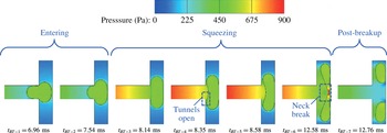
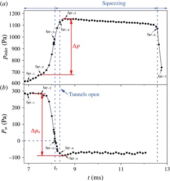
Compared with the breakup with permanent obstruction, the breakup of the droplet with tunnels exhibits similar dynamic behaviours in the entering and post-breakup stages, but not in the squeezing stage, as shown in figures 11 and 12. As indicated, unlike the breakup with permanent obstruction, two tunnels appear between the sidewalls and the droplet at
 $t_{BT-4}=8.35$
ms in the initial period of the squeezing stage. However, similar to the breakup with permanent obstruction,
 $p_{inlet}$
continues to increase drastically during this period, which mainly drives the increasing concavity of the rear (see
 $t_{BT-3}$
–
 $t_{BT-5}$
in figure 12
a). This implies that the effect of tunnels is not obvious at this moment. Note that, after the moment
 $t_{BT-5}$
, although the shrinkage and elongation of the neck continues, the curvature radius of the rear and the corresponding
 $p_{\unicode[STIX]{x1D70E}}$
remain the same, which is different from the case of breakup with permanent obstruction. The steady evolution of
 $p_{\unicode[STIX]{x1D70E}}$
lasts to the end of the squeezing stage just before the breakup of the droplet. Thereafter, the upstream pressure returns to normal immediately (see figure 12
a).
Evolution of the pressure field for droplet breakup with tunnels in a T-junction (
 $\unicode[STIX]{x1D706}=1/8$
,
 $Ca=0.05$
,
 $l_{0}/w=2.33$
).

Evolution of the pressure for droplet breakup with tunnels (
 $\unicode[STIX]{x1D706}=1/8$
,
 $Ca=0.05$
,
 $l_{0}/w=2.33$
): (a) the inlet pressure of the main channel, (b) the Laplace pressure of the rear droplet interface (negative values signify that the surface tension is oriented upstream).

Evolution of the dimensionless characteristic parameters in the squeezing stage (
 $t^{\ast }=(t-t_{c})U/w$
,
 $\unicode[STIX]{x1D706}=1/8$
,
 $Ca=0.05$
,
 $l_{0}/w=2.33$
): (a) the neck thickness, inset: the same data as
 $\log (1-\unicode[STIX]{x1D6FF}^{\ast })$
versus
 $\log (t^{\ast })$
; (b) the distance travelled by the tip of the droplet, inset: the same data as
 $\log (\unicode[STIX]{x0394}l_{t}^{\ast })$
versus
 $\log (t^{\ast })$
; (c) the thickness of the film sandwiched between droplet and channel walls.

To explore the effect of tunnels on the dynamic behaviours of droplets, figure 13 shows the evolution of three dimensionless geometrical parameters in the squeezing stage. Similar to the breakup with permanent obstruction, the evolution of
 $1-\unicode[STIX]{x1D6FF}^{\ast }$
can also be divided into the first substage with a linear relationship and the second substage with an exponential relationship (see inset in figure 13
a). However, the exponent of the second substage is about
 $2/7$
, which is smaller than
 $3/7$
when the droplet breaks up with permanent obstruction. It can be concluded that owing to the appearance of tunnels, the droplet deformation is weakened with a slower squeezing speed. In other words, the shear stresses due to the lubricating flow in the tunnel play a small role in the elongation of the droplet. In conjunction with figure 12, the slower squeezing speed should be caused by the large, stable resistance due to surface tension. As seen in figure 13(b), the trend of the distance travelled by the tip of the droplet changes from a linear relationship to an exponential one with an exponent
 $3/7$
(see the inset in figure 13
b). A similar trend is also reported by Wang et al. (Reference Wang, Zhu, Wu, Fu and Ma2015) when bubbles break up in a T-junction with tunnels. This evolutionary trend demonstrates that the appearance of tunnels slows down the droplet elongation during the squeezing stage. In this case, the characterized parameter
 $d$
exceeds the interface thickness at the opening point of the tunnel
 $t_{BT-4}$
(see figure 13
c) and increases to a maximum value, which is related to
 $Ca$
(Jullien et al.
Reference Jullien, Tsang Mui Ching, Cohen, Menetrier and Tabeling2009). It is interesting to note that the maximum
 $d$
remains unchanged until breakup occurs, which is related to the above stable Laplace pressure region shown in figure 12(b).
4.1.3 Non-breakup
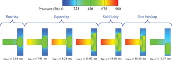
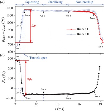
When the droplet does not break up through the T-junction, it experiences similar entering and squeezing stages and different stabilizing and non-breakup stages, as depicted in figures 14 and 15. As shown in figure 14, from the moment
 $t_{NB-4}$
= 11.02 ms, the droplet stops elongating and attains a stable state under the symmetry conditions. During the stabilizing stage,
 $p_{inlet}$
and
 $p_{\unicode[STIX]{x1D70E}}$
both stay unchanged (see figure 15). This stage lasts to
 $t_{NB-5}$
= 14.5 ms, when a random disturbance is imposed at the outlet I. After that, the pressure of outlet I gradually increases and becomes larger than that of outlet II (see figure 15
a). Due to the pressure instability, the droplet starts to lose its balance. At the beginning of the non-breakup stage, it has little influence on
 $p_{\unicode[STIX]{x1D70E}}$
between
 $t_{NB-5}$
and
 $t_{NB-6}$
(see figure 15
b). But when it reaches
 $t_{NB-6}$
= 18.10 ms, the tip of the non-breakup droplet starts to cross the axis of symmetry and the balance is completely broken. After that, the droplet quickly escapes through one daughter channel without breakup, which brings dramatic changes to
 $p_{\unicode[STIX]{x1D70E}}$
and the upstream pressure (see figure 15
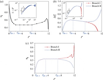
b). In addition, figure 16 shows the evolution of three dimensionless geometrical parameters when droplets do not break up. As shown in the figures, the thicknesses of the neck and tunnel are both unchanged as
 $t_{NB-4}<t<t_{NB-5}$
and only the elongation length of the droplet decreases slightly, which may be due to the surface tension at the tips of the droplet.
Evolution of the pressure field for droplet non-breakup in a T-junction (
 $\unicode[STIX]{x1D706}=1/8$
,
 $Ca=0.05$
,
 $l_{0}/w=2.13$
).

Evolution of the pressure for the case of droplet non-breakup (
 $\unicode[STIX]{x1D706}=1/8$
,
 $Ca=0.05$
,
 $l_{0}/w=2.13$
): (a) the pressure drop of the inlet and outlet, (b) the Laplace pressure of the rear droplet interface (negative values signify that the surface tension is oriented upstream).

Evolution of the dimensionless characteristic parameters (
 $t^{\ast }=(t-t_{c})U/w$
,
 $\unicode[STIX]{x1D706}=1/8$
,
 $Ca=0.05$
,
 $l_{0}/w=2.13$
): (a) the neck thickness, inset: the same data as
 $\log (1-\unicode[STIX]{x1D6FF}^{\ast })$
versus
 $\log (t^{\ast })$
; (b) the distance travelled by the tip of the droplet, inset: the same data as
 $\log (\unicode[STIX]{x0394}l_{t}^{\ast })$
versus
 $\log (t^{\ast })$
; (c) the thickness of the film sandwiched between droplet and channel walls.

4.1.4 Critical neck thickness and minimal film thickness
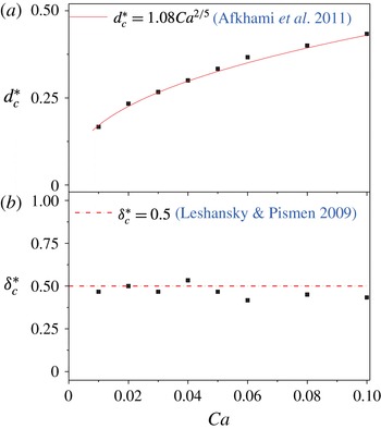
The critical minimal film thickness and neck thickness at various capillary numbers for the non-breakup droplets adjacent to the breakup threshold: (a) critical minimal film thickness
 $d_{c}^{\ast }$
,
 $d_{c}^{\ast }=d_{c}/w$
; (b) critical neck thickness
 $\unicode[STIX]{x1D6FF}_{c}^{\ast }$
,
 $\unicode[STIX]{x1D6FF}_{c}^{\ast }=\unicode[STIX]{x1D6FF}_{c}/w$
.

When droplets do not break up, the dimensionless characteristic parameters – neck thickness
 $\unicode[STIX]{x1D6FF}^{\ast }$
and minimal film thickness
 $d^{\ast }$
between droplet and channel walls – exhibit different evolutions from those in the breakup situations (see figures 10, 13 and 16). The non-breakup droplets adjacent to the breakup threshold have the critical neck thickness
 $\unicode[STIX]{x1D6FF}_{c}^{\ast }$
and minimal film thickness
 $d_{c}^{\ast }$
, as was first proposed by Leshansky & Pismen (Reference Leshansky and Pismen2009). According to the analytical theory of Leshansky & Pismen (Reference Leshansky and Pismen2009), the critical neck thickness is estimated as
 $\unicode[STIX]{x1D6FF}_{c}^{\ast }=\unicode[STIX]{x1D6FF}_{c}/w=0.5$
, and the relation between critical minimal film thickness and capillary number is predicted as
 $d_{c}^{\ast }=d_{c}/w=1.08Ca^{2/5}$
(Afkhami et al.
Reference Afkhami, Leshansky and Renardy2011), which has also been validated by the other experimental and numerical studies (Jullien et al.
Reference Jullien, Tsang Mui Ching, Cohen, Menetrier and Tabeling2009; Afkhami et al.
Reference Afkhami, Leshansky and Renardy2011). Herein, the present numerical values of
 $\unicode[STIX]{x1D6FF}_{c}^{\ast }$
and
 $d_{c}^{\ast }$
at various capillary numbers are also compared with this theoretical prediction (see figure 17). As expected, the numerical values of the two critical parameters agree well with the theoretical ones, which further indicates the reliability of the present model.
4.2 Roles of shear stress and vortex in droplet deformation
As mentioned above, in the non-breakup case, the droplet experiences a key stabilizing stage with no elongation and two tunnels open, which provides a precondition for the final non-breakup. However, why this key stabilizing stage appears remains unclear. Therefore, further research is performed here to understand why the squeezing phenomenon slows down or stops with the appearance of tunnels.
Note that, generally, the shear stress is deemed to promote stretching and breakup of a droplet in an unbounded geometry (Zhou & Pozrikidis Reference Zhou and Pozrikidis1993; Roths et al. Reference Roths, Friedrich, Marth and Honerkamp2002). However, according to the above results shown in figures 11–16, the shear action due to the lubricating flow in the tunnels actually slows down and even stops the elongation of the droplet during the squeezing stage of droplet non-breakup processes. Therefore, the role of the shear action remains unclear and needs to be further examined, particularly for the non-breakup condition. Additionally, the vortex flow formed with the appearance of tunnels has recently started to attract attention (Afkhami et al. Reference Afkhami, Leshansky and Renardy2011), though it is somewhat less discussed, and it is also acknowledged as an important resistance to droplet deformation (Rallison Reference Rallison1984). Therefore, in order to elucidate the real effect of tunnels on droplet non-breakup behaviour through the microfluidic T-junction, two hydrodynamic parameters – shear stress and vorticity – are investigated and analysed in this section.
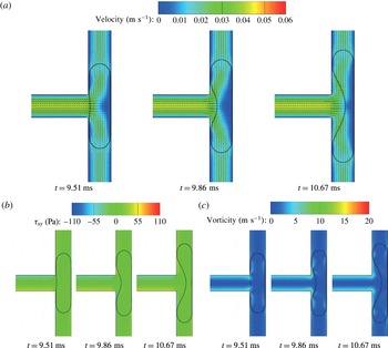
Evolution of the droplet breakup with permanent obstruction in a T-junction during the squeezing stage (
 $\unicode[STIX]{x1D706}=1/8$
,
 $Ca=0.05$
,
 $l_{0}/w=3.73$
): (a) velocity, (b) shear stress and (c) vorticity.

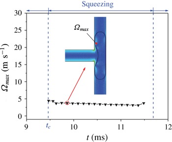
Evolution of the maximum vorticity in the droplet during the breakup with permanent obstruction (
 $\unicode[STIX]{x1D706}=1/8$
,
 $Ca=0.05$
,
 $l_{0}/w=3.73$
).

As a comparison, figure 18 depicts the evolution of the velocity, shear stress and vorticity fields when the channels are permanently obstructed. Additionally, figure 19 quantizes the evolution of the maximum vorticity during this process. As shown, all three fields exhibit a non-obvious variation during this process. The maximum vorticity in the droplet is small and remains around
 $\unicode[STIX]{x1D6FA}_{max}=3.39~\text{ms}^{-1}$
. Owing to the absence of a lubricating film between the droplet and channel walls, the shear stress acting on the tip of the droplet can actually be ignored. Accordingly, in this situation without the tunnel effect, the buildup of upstream pressure chiefly drives the breakup process by overcoming the deformation resistance through the interface tension of the rear.
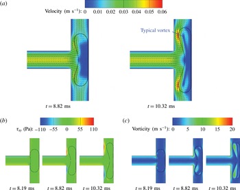
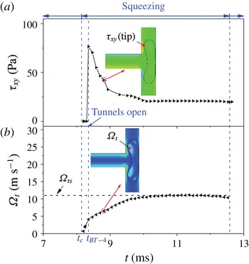
When droplets break up with tunnels, the velocity, shear stress and vorticity fields show some difference from the breakup with permanent obstruction, due to the appearance of tunnels. As seen in figure 20(a), the tunnels induce a continuous flow of fluid to develop between the tips of the droplet and the sidewalls. This flow generates shear stresses at the tips of the droplet, which produces two typical vortices inside the tips (see figure 20 a). As the process goes on, the vorticity of the typical vortex increases until the droplet breaks (see figure 20 c). As seen in figure 20(b), the shear stress around the tip of the droplet is small and not as significant as that near the sidewalls.
Evolution of the droplet breakup with tunnels in a T-junction during the squeezing stage (
 $\unicode[STIX]{x1D706}=1/8$
,
 $Ca=0.05$
,
 $l_{0}/w=2.33$
): (a) velocity, (b) shear stress, (c) vorticity.

Evolution of the shear stress and vorticity for droplet breakup with tunnels (
 $\unicode[STIX]{x1D706}=1/8$
,
 $Ca=0.05$
,
 $l_{0}/w=2.33$
): (a) the shear stress acting on the tip of the droplet, (b) the vorticity of a typical vortex in the droplet.

Figure 21(a) quantitatively depicts the evolution of the shear stress acting on the tip of the droplet. As mentioned above, when the channels are blocked, the shear stress acting on the tips of the droplet can be ignored, i.e. it is approximately equal to 0. After tunnels appear, this shear stress decreases as the tunnels open and finally reaches a steady value. On the other hand, the shear action in the tunnels activates vortices inside the tips of the droplet after opening of the tunnels at
 $t_{BT-4}$
. Moreover, corresponding to the decrease in shear stress, the vorticity of the vortices increases over time and finally reaches a steady value (see
 $\unicode[STIX]{x1D6FA}_{ts}=11.0~\text{ms}^{-1}$
in figure 21
b), implying that a part of the momentum in shear transits into that of vortices. In particular, these vortices have been well demonstrated to highly inhibit droplet deformation (Rallison Reference Rallison1984), which can exactly explain why the appearance of tunnels slows down the elongation of droplets. Therefore, it can be concluded that, rather than facilitating the elongation, shear effects in the tunnels actually induce the vortices inside the tips of the droplet, which contributes to resisting elongation of the droplet (see figure 13
a,b).
Evolution of the droplet non-breakup process in a T-junction (
 $\unicode[STIX]{x1D706}=1/8$
,
 $Ca=0.05$
,
 $l_{0}/w=2.13$
): (a) velocity, (b) shear stress, (c) vorticity.

Evolution of the shear stress and vorticity for the case of droplet non-breakup (
 $\unicode[STIX]{x1D706}=1/8$
,
 $Ca=0.05$
,
 $l_{0}/w=2.13$
): (a) the shear stress acting on the tip of the droplet, (b) the vorticity of a typical vortex in the droplet.

Evolution of the final steady vorticity and deformation rate with droplet size (
 $\unicode[STIX]{x1D706}=1/8$
,
 $Ca=0.05$
).

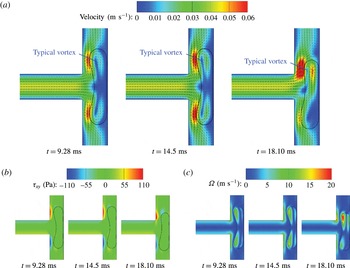
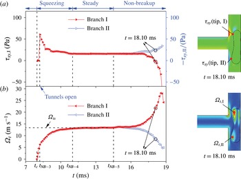
As shown in figure 22, as the initial droplet length decreases, the droplet would stop elongating and reach a steady state located at the middle of a T-junction under conditions of symmetry, when the droplet does not break up. Similarly to figure 20, vortex flows are formed, which inhibits deformation of the droplet. Quantitative descriptions are given in figure 23 to provide detailed information. It is indicated that the shear stress and vorticity are both unchanged in the stabilizing stage. Moreover, the final steady vorticity in the non-breakup case is
 $\unicode[STIX]{x1D6FA}_{ts}=13.3~\text{ms}^{-1}$
, which is larger than
 $\unicode[STIX]{x1D6FA}_{ts}=11.0~\text{ms}^{-1}$
when the droplet breaks up with tunnels.
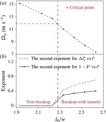
To further understand the role of vorticity as tunnels appear, figure 24 presents the evolution of the final steady vorticity and deformation rate (characterized by the evolution exponents of
 $1-\unicode[STIX]{x1D6FF}^{\ast }$
and
 $\unicode[STIX]{x0394}l_{t}^{\ast }$
in the second substage during squeezing) versus droplet size. In the figures, as the initial droplet length reduces, the final steady vorticity
 $\unicode[STIX]{x1D6FA}_{ts}$
gradually increases, which contributes to the decrease in droplet deformation rate. This negative relationship further demonstrates the inhibiting effect of the vortex on the droplet breakup. Once
 $\unicode[STIX]{x1D6FA}_{ts}$
exceeds a critical value, the evolution exponents become equal to zero and the droplet will no longer break up. In the figure, the critical
 $\unicode[STIX]{x1D6FA}_{ts}$
is between 11.0
 $\text{ms}^{-1}$
and 12.7
 $\text{ms}^{-1}$
when
 $\unicode[STIX]{x1D706}=1/8$
and
 $Ca=0.05$
.
According to the above analysis, the mechanism of droplet breakup or non-breakup can be concluded as follows. When the droplet permanently obstructs the daughter channels, its elongation is driven by the buildup of pressure upstream and resisted by the forces of surface tension. If the droplet elongates with tunnels, the vortex flow formed in the tips of the droplet provides an additional resistance to droplet deformation, which slows down the droplet deformation rate before breakup occurs. In particular, when the strength of the vortex flow exceeds the critical value, the droplet does not break up. Therefore, the vortex flow plays an important role in determining whether breakup or non-breakup occurs.
4.3 Phase diagram of droplet behaviour in the microfluidic T-junction
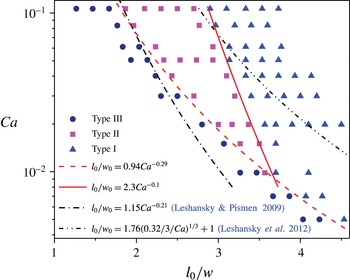
Phase diagram of droplet behaviours through the T-junction (
 $w_{0}=w_{1}=w,\unicode[STIX]{x1D706}=1/8$
). Type I: breakup with permanent obstruction; type II: breakup with tunnels; type III: non-breakup.

Figure 25 displays the phase diagram for droplet behaviours through the T-junction, the characteristics of which are similar to those of previous work (Link et al.
Reference Link, Anna, Weitz and Stone2004; Jullien et al.
Reference Jullien, Tsang Mui Ching, Cohen, Menetrier and Tabeling2009; Leshansky & Pismen Reference Leshansky and Pismen2009; Fu et al.
Reference Fu, Ma, Funfschilling and Li2011; Leshansky et al.
Reference Leshansky, Afkhami, Jullien and Tabeling2012). Note that, by means of the lubrication analysis method, Leshansky et al. made theoretical predictions of the threshold between different flow patterns (Leshansky & Pismen Reference Leshansky and Pismen2009; Leshansky et al.
Reference Leshansky, Afkhami, Jullien and Tabeling2012). They found that the critical threshold between types III and II has a dependence on the capillary number, i.e.
 $l_{0}/w\sim Ca^{-1/5}$
, which is approximately expressed as
 $l_{0}/w=\unicode[STIX]{x1D6FD}Ca^{-0.21}$
(Leshansky & Pismen Reference Leshansky and Pismen2009). In accordance with this threshold relationship, several other researchers (Jullien et al.
Reference Jullien, Tsang Mui Ching, Cohen, Menetrier and Tabeling2009; Fu et al.
Reference Fu, Ma, Funfschilling and Li2011) fitted the best
 $\unicode[STIX]{x1D6FD}$
with different values based on their respective experimental and numerical data. On the other hand, for the threshold between types II and I, the formula is given by
 $l_{0}/w=1.76(\unicode[STIX]{x1D6FC}/3Ca)^{1/3}+1$
(Leshansky et al.
Reference Leshansky, Afkhami, Jullien and Tabeling2012). Therefore, we also adopt these threshold formulas and fit them according to the present numerical data. Herein, we obtain the best fitting thresholds with
 $\unicode[STIX]{x1D6FD}=1.15$
for the threshold between types III and II and
 $\unicode[STIX]{x1D6FC}=0.32$
for that between types II and I. The two formulas both describe the boundaries well when
 $Ca$
is large but do not work well for small
 $Ca$
. To predict the fitting threshold on the basis of the present numerical data, we utilize a power-law formula,
 $l_{0}/w=\unicode[STIX]{x1D6FD}Ca^{b}$
, to describe the boundaries between different flow patterns (Fu et al.
Reference Fu, Ma, Funfschilling and Li2011). As shown in figure 25, the power-law formulas used,
 $l_{0}/w=0.94Ca^{-0.29}$
and
 $l_{0}/w=2.3Ca^{-0.1}$
, are in good agreement with the boundaries observed in the present results. Note that as
 $Ca\leqslant 0.01$
, flow type II barely occurs in the present cases. A similar situation can also be found in the work of Jullien et al. (Reference Jullien, Tsang Mui Ching, Cohen, Menetrier and Tabeling2009).
4.4 Effect of viscosity ratio on droplet behaviour through the microfluidic T-junction
Previous studies have shown that the viscosity ratio between continuous and disperse phases plays an important role in the droplet behaviours through the microfluidic T-junction (De Menech Reference De Menech2006; Jullien et al.
Reference Jullien, Tsang Mui Ching, Cohen, Menetrier and Tabeling2009; Afkhami et al.
Reference Afkhami, Leshansky and Renardy2011; Fu et al.
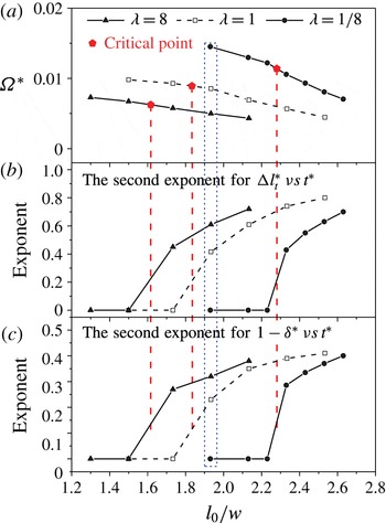
Reference Fu, Ma, Funfschilling and Li2011). Accordingly, the effect of viscosity ratio on the droplet hydrodynamics through the microfluidic T-junction, including the dimensionless steady vorticity
 $\unicode[STIX]{x1D6FA}^{\ast }=w\unicode[STIX]{x1D6FA}_{ts}/U$
, droplet deformation rates and phase diagrams, is further numerically investigated here by varying the viscosity of the droplet
 $\unicode[STIX]{x1D702}_{w}$
while keeping the viscosity of the continuous fluid
 $\unicode[STIX]{x1D702}_{o}$
constant. Based on the numerical simulation, the evolutions of the dimensionless steady vorticity and deformation rates with droplet size are depicted in figure 26. It can be seen that the droplet with larger viscosity induces a smaller dimensionless steady vorticity (see figure 26
a) and larger deformation rates (see figure 26
b,c). This is attributed to the fact that a large droplet viscosity results in a small velocity gradient in the droplet under the same shear action of continuous flow, which restricts the vortex generation. Note that a small vorticity produces little deformation resistance, and thus enlarges the droplet deformation. In addition, in this situation, the droplet with larger viscosity is more easily broken up, which is also proven by the fact that the critical
 $\unicode[STIX]{x1D6FA}^{\ast }$
decreases with increasing viscosity ratio (see figure 26
a).
The evolution of the dimensionless steady vorticity and deformation rates with droplet size for three different fluid viscosity ratios (
 $w_{0}=w_{1}=w$
,
 $Ca=0.05$
,
 $\unicode[STIX]{x1D6FA}^{\ast }=w\unicode[STIX]{x1D6FA}_{ts}/U$
).

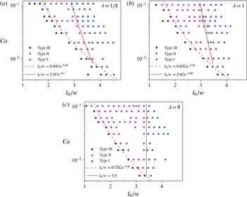
Phase diagrams of droplet behaviours through the T-junction for three different fluid viscosity ratios (
 $w_{0}=w_{1}=w$
). Type I: breakup with permanent obstruction; type II: breakup with tunnels; type III: non-breakup.

Furthermore, figure 27 presents the phase diagrams of droplet behaviours through the T-junction for different viscosity ratios. As shown, the boundaries between the flow patterns for type I (breakup with permanent obstruction) and type II (breakup with tunnels) are slightly changed with varying viscosity ratio, especially at small capillary numbers. This indicates that the viscosity ratio has a slight effect on the droplet behaviours when channels are permanently obstructed. In contrast, the boundaries between breakup and non-breakup shift significantly to small
 $l_{0}/w$
with increasing viscosity ratio, which is consistent with the numerical results (De Menech Reference De Menech2006; Afkhami et al.
Reference Afkhami, Leshansky and Renardy2011) and experimental results (Jullien et al.
Reference Jullien, Tsang Mui Ching, Cohen, Menetrier and Tabeling2009; Fu et al.
Reference Fu, Ma, Funfschilling and Li2011). This further indicates that the droplet with larger viscosity is more easily broken up.
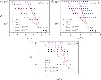
4.5 Effect of width ratio on droplet behaviour through the microfluidic T-junction
In addition to the viscosity ratio between continuous and disperse phases, the width ratio of the T-junction
 $w_{1}/w_{0}$
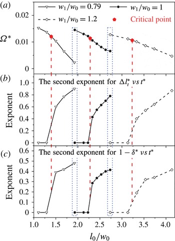
also has a significant impact on droplet behaviours. Therefore, in order to quantitatively explore the influence of
 $w_{1}/w_{0}$
on the droplet behaviours, the evolutions of steady vorticity and deformation rates are studied at three different width ratios by changing the branch channel width
 $w_{1}$
for a fixed size of the main channel (see figure 28). As shown in figure 28, when the width ratio
 $w_{1}/w_{0}$
becomes small, the evolutionary curves all move towards small
 $l_{0}/w_{0}$
, implying that
 $\unicode[STIX]{x1D6FA}^{\ast }$
decreases and deformation rate increases with decreasing
 $w_{1}/w_{0}$
. This phenomenon implies that smaller branch channels induce easier droplet deformation and breakup. It is worth noting that although the width ratio varies, the critical
 $\unicode[STIX]{x1D6FA}^{\ast }$
has barely changed (see figure 28
a).
Additionally, phase diagrams of droplet behaviours through the T-junction for different width ratios are also depicted in figure 29. As shown, the two boundaries between the three flow patterns both shift towards small
 $l_{0}/w_{0}$
with decreasing
 $w_{1}/w_{0}$
. These results are attributed to the fact that a droplet in small branch channels tends to obstruct them and generate small vortex flows, which induce easier break-up of the droplet. Therefore, reducing the width ratio
 $w_{1}/w_{0}$
would help to break up the droplet through the T-junction. In addition, as shown in figure 29, the boundaries between breakup and non-breakup for the cases with different width ratio all follow the power law with the same exponent
 $-0.29$
.
The evolution of the dimensionless steady vorticity and deformation rates with droplet size for three different width ratios (
 $\unicode[STIX]{x1D706}=1/8$
,
 $Ca=0.05$
,
 $\unicode[STIX]{x1D6FA}^{\ast }=w_{1}\unicode[STIX]{x1D6FA}_{ts}/U$
).

Phase diagrams of droplet behaviours through the T-junction for three different width ratios (
 $\unicode[STIX]{x1D706}=1/8$
). Type I: breakup with permanent obstruction; type II: breakup with tunnels; type III: non-breakup.

5 Conclusions
In summary, we have developed a phase-field multiphase lattice Boltzmann model to systematically investigate droplet dynamic behaviours through a microfluidic T-junction, focusing especially on the non-breakup of the droplet.
Firstly, we systematically present and compare the detailed information on breakup and non-breakup, including the quantitative evolutions of driving and resistance forces and droplet deformation characteristics involved. It is indicated that, under a symmetric boundary condition, non-breakup droplets finally stop elongating and reach a stable stage, where the upstream pressure and resistance from surface tension reach stable values too. Through detailed comparisons between the cases of non-breakup and breakup, we find that the appearance of tunnels provides a precondition for the final non-breakup of droplets. The tunnel effect would slow down the droplet deformation rate and even induce non-breakup of the droplet in the T-junction. This effect on droplet deformation can be deduced from the evolutions of the dimensionless characteristic parameters involved (i.e. the neck thickness, distance travelled by the tips of the droplet and the thickness of film sandwiched between droplet and channel walls) for non-breakup and breakup cases. In addition, the present numerical results, such as for critical neck thickness
 $\unicode[STIX]{x1D6FF}_{c}^{\ast }$
and minimal film thickness
 $d_{c}^{\ast }$
, are also compared with previous studies (Jullien et al.
Reference Jullien, Tsang Mui Ching, Cohen, Menetrier and Tabeling2009; Leshansky & Pismen Reference Leshansky and Pismen2009; Afkhami et al.
Reference Afkhami, Leshansky and Renardy2011), which validates the reliability of the present model.
Then, further research is performed to explore the roles of shear stress and vorticity on the dynamic behaviours of droplets through the T-junction. It is found that the shear action in the tunnels contributes little to the droplet elongation in the flow patterns with tunnels. On the other hand, the vortex flow formed in the droplet plays an important role in determining whether the droplet breaks up or not. In particular, when the strength of vortex flow exceeds a critical value, the droplet will no longer break up. Accordingly, more effort has been devoted to investigating the effects of viscosity ratio between disperse and continuous phases and width ratio between branch and main channels on the droplet dynamic behaviours through the T-junctions. It is found that under the same shear action of continuous flow, large droplet viscosity results in a small velocity gradient in the droplet, which restricts the vortex generation and thus produces smaller deformation resistance. Consequently, a droplet with larger viscosity is more easily broken up. Our work also reveals that a droplet in small branch channels tends to obstruct the channels and generate small vortex flows, which induces easier break-up of the droplet. Finally, based on the numerical results in this work, we plot several phase diagrams to represent the various flow patterns of droplets, including breakup with permanent obstruction, breakup with tunnels and non-breakup, depending on capillary number, droplet size, viscosity ratio between disperse and continuous phases, and geometry of the T-junction. Furthermore, the corresponding power-law correlations in the form
 $l_{0}/w=\unicode[STIX]{x1D6FD}Ca^{b}$
are fitted to describe the boundaries between different flow patterns of droplets.
Acknowledgement
This work was supported by NSAF (no. U1530260) and 333 Project of Jiangsu Province in China.