1. Introduction
Global Navigation Satellite Systems (GNSS), with the Global Positioning System (GPS) as the most prominent example, have become essential infrastructure for positioning, navigation and timing across a wide range of applications, from autonomous vehicles to precision agriculture. Achieving high-accuracy state estimation from GPS observables, however, remains a persistent challenge, as real-world observation environments routinely introduce non-Gaussian noise through multipath propagation, signal blockage in urban canyons and atmospheric disturbances (Brown and Hwang, Reference Brown and Hwang1997).
The Kalman filter (KF) provides the minimum mean square error optimal estimate for linear systems under Gaussian noise assumptions. In GPS navigation, however, the pseudorange measurement model is inherently nonlinear, motivating the use of the extended Kalman filter (EKF). By linearising the nonlinear state and measurement equations through first-order Taylor expansion, the EKF enables recursive state estimation for nonlinear systems (Izanloo et al., Reference Izanloo, Fakoorian, Yazdi and Simon2016). Nevertheless, because its update mechanism is still based on second-order error statistics, the EKF remains sensitive to heavy-tailed noise and impulsive outliers, and its estimation performance can degrade significantly in non-Gaussian environments.
To improve robustness under such conditions, information-theoretic learning (ITL) criteria have been introduced as alternatives to the conventional minimum mean square error (MMSE)-based framework. The maximum correntropy criterion (MCC) is an ITL approach based on correntropy and kernel-induced local similarity, which suppresses the influence of large estimation errors through a kernel-weighted objective function (Principe, Reference Principe2010; Rényi, Reference Rényi1961). Based on this concept, Liu et al. (Reference Liu, Qu, Zhao and Chen2016) and Chen et al. (Reference Chen, Liu, Zhao and Principe2017) developed the maximum correntropy criterion-based extended Kalman filter (MCC-EKF), demonstrating improved robustness over the conventional EKF in non-Gaussian environments. Subsequent extensions further expanded MCC-based filtering to multi-kernel and regression-based formulations (Chen et al., Reference Chen, Xie, Wang, Yuan, Ren and Qin2022; Liu et al., Reference Liu, Ren, Lyu, Jiang, Ren and Chen2021). Another representative approach is the minimum error entropy (MEE) criterion, which minimises the entropy of the estimation error rather than relying only on its second-order moment, thereby incorporating higher-order statistical information into the filtering process. Based on this, Chen et al. (Reference Chen, Dang, Gu, Zheng and Principe2019) proposed the MEE-EKF, and subsequent studies extended this framework to fiducial-point-based cubature and dual-EKF architectures. In particular, Dang and Chen (Reference Dang and Chen2022a) developed the minimum error entropy with fiducial points cubature Kalman filter (MEEF-CKF) for INS/GPS integration under complex non-Gaussian noise, while Dang and Chen (Reference Dang and Chen2022b) extended the MEEF framework to a dual EKF architecture for joint state and parameter estimation. Numerically stable MEE-based implementations have also been investigated to improve robustness and convergence behaviour in practical filtering problems (Gang et al., Reference Gang, Chen, Yang, Peng and Feng2021). More recently, the MEEF framework has been extended to distributed and adaptive state-estimation problems. Zhao and Tian (Reference Zhao and Tian2025) developed a distributed MEEF-based Kalman filtering framework for state tracking under complex non-Gaussian noise, and Wang and Wang (Reference Wang and Wang2025) proposed an adaptive MEEF-KF for SINS/USBL integrated navigation under non-Gaussian measurement disturbances. However, MCC-based filters may become less effective when a fixed kernel bandwidth is used under rapidly varying noise conditions, while MEE-based filters may suffer from numerical instability or degraded convergence behaviour in dynamic scenarios (Dang and Chen, Reference Dang and Chen2022b).
To address these limitations, Yang et al. (Reference Yang, Cao, Ran and Xiao2021a, Reference Yang, Cao, Li, Jiang, Ran and Xiao2021b) proposed the centred error entropy (CEE) criterion by combining the strengths of MCC and MEE within a unified information-theoretic framework. By integrating correntropy-based local similarity and entropy-based error concentration, the CEE criterion provides improved robustness and estimation stability in nonlinear systems affected by non-Gaussian noise. The CEE-EKF has demonstrated superior performance compared with both MCC-EKF and MEE-EKF in nonlinear, non-Gaussian filtering problems (Yang et al., Reference Yang, Cao, Ran and Xiao2021a, Reference Yang, Cao, Li, Jiang, Ran and Xiao2021b). Moreover, the CEE criterion has been applied to GNSS multipath estimation by Cheng et al. (Reference Cheng, Ren and Xie2016), satellite attitude determination by Yang et al. (Reference Yang, Cao, Ran and Xiao2021a) and spacecraft state estimation using sigma-point Kalman filtering by Yang et al. (Reference Yang, Huang and Cao2022). These applications further support the potential of CEE-based filtering for robust navigation and state estimation under disturbed observation conditions.
In addition to information-theoretic filtering methods, this study includes other robust and adaptive EKF-based approaches as additional baseline methods for non-Gaussian navigation state estimation. The Student’s t-based extended Kalman filter (ST-EKF) enhances robustness by modelling measurement uncertainty with a heavy-tailed Student’s t distribution, making it more tolerant of outliers than the Gaussian model. In the study by Huang and Zhang (Reference Huang and Zhang2017, Reference Huang and Zhang2022), a Student’s t-based EKF benchmark was developed based on the heavy-tailed modelling principle. The variational Bayesian extended Kalman filter (VB-EKF), however, adaptively estimates noise statistics by treating the noise covariance as an unknown latent variable and updating it within a Bayesian inference framework (Chen et al., Reference Chen, Zhu and Leung2026). While the ST-EKF is effective for modelling heavy-tailed noise and the VB-EKF is advantageous in time-varying noise environments, their effectiveness still relies on the assumed probabilistic model and inference framework. In contrast, the CEE-EKF enhances robustness from an information-theoretic standpoint without requiring a predefined noise distribution, making it well suited for applications involving uncertain and complex non-Gaussian disturbances.
Despite substantial progress in robust nonlinear filtering, comprehensive comparisons among these filter families within a unified GPS state estimation framework remain limited. Most existing studies evaluate individual methods separately or under relatively restricted noise settings. To provide a more systematic assessment, this study compares six EKF-based methods, namely the EKF, MEE-EKF, MCC-EKF, ST-EKF, VB-EKF and CEE-EKF, for GPS state estimation under non-Gaussian noise conditions. The CEE-EKF is treated as the primary method of interest, while the other filters serve as representative benchmark methods spanning conventional, information-theoretic, robust and adaptive estimation strategies.
The remainder of this paper is organised as follows. Section 2 provides a brief review of the extended Kalman filter based on the maximum correntropy criterion. Section 3 introduces the extended Kalman filter based on minimum error entropy. Section 4 presents the centred error entropy extended Kalman filter. Section 5 reviews selected representative robust and adaptive filters, excluding kernel-based information-theoretic methods, with particular emphasis on ST-EKF and VB-EKF. Section 6 evaluates the performance of the proposed method in comparison with these techniques using illustrative examples from both simulation and field test data. Finally, Section 7 presents the conclusions and outlines directions for future work.
2. The extended Kalman filter based on maximum correntropy criterion
Correntropy is a nonlinear similarity measure that quantifies the local structure between two random variables via kernel density estimation, offering inherent robustness to non-Gaussian noise and outliers that the conventional mean-square-error (MSE) criterion cannot provide (Izanloo et al., Reference Izanloo, Fakoorian, Yazdi and Simon2016; Liu et al., Reference Liu, Qu, Zhao and Chen2016). Given random variables
 $X$
and
 $Y$
with joint distribution
 ${f_{XY}}(x,y)$
, the correntropy is defined as
 $${V_\sigma }{\rm{(}}X,Y{\rm{)}} = E{\rm{[}}{\kappa _\sigma }{\rm{(}}X,Y{\rm{)]}} = \mathop{ \int \! \int} \limits_{\! x \in X,y \in Y} {{\kappa _\sigma }{\rm{(}}x,y{\rm{)}}{f_{XY}}(x,y)dxdy}$$
where
 ${\kappa _\sigma }{\rm{(}} \!\cdot \!{\rm{)}}$
denotes a kernel function dependent on the difference between
 $X$
and
 $Y$
, and
 $\sigma $
is the kernel bandwidth. The Gaussian kernel is most commonly adopted, given by
 $${\kappa _\sigma }(X,Y) = {G_\sigma }(e) = \exp ( - {{{e^2}} \over {2{\sigma ^2}}})$$
where
 $e = x - y$
. As
 $\sigma \to \infty $
, correntropy becomes equivalent to the MSE criterion. For finite
 $\sigma $
, large errors are exponentially downweighted, thereby enhancing robustness. Since the joint distribution
 ${f_{XY}}$
is generally unknown, correntropy is approximated using
 $N$
samples as
 $${\hat V_\sigma }\left( {X,Y} \right) = {1 \over N}\sum\limits_{i = 1}^N {{G_\sigma }} ({e_i}) = {1 \over N}\sum\limits_{i = 1}^N {{G_\sigma }\left( {{x_i} - {y_i}} \right)} $$
Maximising Equation (3) instead of minimising a quadratic cost function enables the MCC framework to effectively suppress the influence of outliers and heavy-tailed noise. Incorporating this principle into the EKF leads to the MCC-EKF, where the prediction step follows the standard EKF formulation, while the measurement update is reformulated as a kernel-weighted optimisation problem.
Consider the following nonlinear discrete-time system model:
 $${{\bf{x}}_k} = f{\bf{(}}{{\bf{x}}_{k - 1}}{\bf{)}} + {{\bf{w}}_{k - 1}}$$
 $${{\bf{z}}_k} = h{\bf{(}}{{\bf{x}}_k}{\bf{)}} + {{\bf{v}}_k}$$
where
 ${{\bf{x}}_k}$
denotes the n-dimensional state vector and
 ${{\bf{z}}_k}$
denotes the m-dimensional measurement vector. Here,
 ${{\bf{w}}_k}$
and
 ${{\bf{v}}_k}$
are mutually uncorrelated zero-mean white noise with covariance matrices
 ${{\bf{Q}}_k}$
and
 ${{\bf{R}}_k}$
, respectively.
Following the standard EKF prediction step, let
 ${{\bf{\hat x}}_{k|k - 1}}$
and
 ${{\bf{P}}_{k|k - 1}}$
denote the one-step predicted state and covariance, respectively. To derive the regression form required for the MCC-based update, the nonlinear measurement equation is linearised around
 ${{\bf{\hat x}}_{k|k - 1}}$
using the first-order Taylor expansion:
 $${{\bf{z}}_k} \approx h{\bf{(}}{{\bf{\hat x}}_{k|k - 1}}{\bf{)}} + {{\bf{H}}_k}{\rm{(}}{{\bf{x}}_k} - {{\bf{\hat x}}_{k|k - 1}}) + {{\bf{v}}_k}$$
Define the one-step prediction error as
 $${{\bf{\varepsilon }}_{k|k - 1}} = {{\bf{x}}_k} - {{\bf{\hat x}}_{k|k - 1}}$$
Then, the augmented model can be written as
 $$\left[ {\matrix{ {{{{\bf{\hat x}}}_{k|k - 1}}} \cr {{{\bf{z}}_k} - h({{{\bf{\hat x}}}_{k|k - 1}}) + {{\bf{H}}_k}{{{\bf{\hat x}}}_{k|k - 1}}} \cr } } \right] = \left[ {\matrix{ {\bf{I}} \cr {{{\bf{H}}_k}} \cr } } \right]{{\bf{x}}_k} + {{\bf{\mu }}_k}$$
where the augmented noise vector is defined as
 $${{\bf{\mu }}_k} = \left[ {\matrix{ { - {{\bf{\varepsilon }}_{k|k - 1}}} \cr {{{\bf{v}}_k}} \cr } } \right]$$
Its covariance is given by
 $$E[{{\bf{\mu }}_k}{\bf{\mu }}_k^{\rm{T}}] = \left[ {\matrix{ {{{\bf{P}}_{k|k - 1}}} & 0 \cr 0 & {{{\bf{R}}_k}} \cr } } \right] = \left[ {\matrix{ {{{\bf{B}}_{{p_{k|k - 1}}}}{\bf{B}}_{{p_{k|k - 1}}}^{\rm{T}}} & 0 \cr 0 & {{{\bf{B}}_{{r_k}}}{\bf{B}}_{{r_k}}^{\rm{T}}} \cr } } \right] = \left[ {\matrix{ {{{\bf{B}}_{p,k|k - 1}}} & 0 \cr 0 & {{{\bf{B}}_{r,k}}} \cr } } \right]{\left[ {\matrix{ {{{\bf{B}}_{p,k|k - 1}}} & 0 \cr 0 & {{{\bf{B}}_{r,k}}} \cr } } \right]^{\rm{T}}} = {{\bf{B}}_k}{\bf{B}}_k^{\rm{T}}$$
where
 ${{\bf{B}}_k}$
is obtained by Cholesky factorisation. Pre-multiplying both sides of the above equation by
 ${\bf{B}}_k^{{\rm{ - 1}}}$
transforms the augmented system into the standardised regression model
 $${{\bf{y}}_k} = {{\bf{W}}_k}{{\bf{x}}_k} + {{\bf{e}}_k}$$
with
 $${{\bf{y}}_k}{\rm{\; = \;}}{\bf{B}}_k^{ - 1}\left[ {\matrix{ {{{{\bf{\hat x}}}_{k|k - 1}}} \cr {{{\bf{z}}_k} - h{\bf{(}}{{{\bf{\hat x}}}_{k|k - 1}}{\bf{)}} + {{\bf{H}}_k}{{{\bf{\hat x}}}_{k|k - 1}}} \cr } } \right],\,{{\bf{W}}_k} = {\bf{B}}_k^{ - 1}\left[ {\matrix{ {\bf{I}} \cr {{{\bf{H}}_k}} \cr } } \right],\,{{\bf{e}}_k} = {\bf{B}}_k^{ - 1}\left[ {\matrix{ { - {{\bf{\varepsilon }}_{k|k - 1}}} \cr {{{\bf{v}}_k}} \cr } } \right]$$
Since the transformed noise vector
 ${{\bf{e}}_k}$
has identity covariance, all residual components are normalised and can therefore be treated uniformly in the MCC formulation. Let
 $L = m + n$
denote the dimension of
 ${{\bf{y}}_k}$
. The MCC objective function is
 $${J_{{\rm{MCC}}}}({{\bf{x}}_k}) = {1 \over L}\sum\limits_{i = 1}^L {{G_\sigma }({{\bf{y}}_{i,k}} - {{\bf{w}}_{i,k}}{{\bf{x}}_k})} $$
where
 ${{\bf{y}}_{i,k}}$
denotes the i-th element of
 ${{\bf{y}}_k}$
, and
 ${{\bf{w}}_{i,k}}$
denotes the i-th row of
 ${{\bf{W}}_k}$
. The optimal state estimate is obtained by maximising Equation (13), that is,
 $${{\bf{\hat x}}_k} = \arg \mathop {\max }\limits_{{{\bf{x}}_k}} {J_{{\rm{MCC}}}}({{\bf{x}}_k}) = \arg \mathop {\max }\limits_{{{\bf{x}}_k}} \sum\limits_{i = 1}^L {{G_\sigma }{\rm{(}}{{\bf{e}}_{i,k}}{\rm{)}}} $$
with the residual defined as
 $${{\bf{e}}_{i,k}} = {{\bf{y}}_{i,k}} - {{\bf{w}}_{i,k}}{{\bf{x}}_k}$$
Setting the gradient of
 ${J_{{\rm{MCC}}}}({{\bf{x}}_k})$
with respect to
 ${{\bf{x}}_k}$
equal to zero, the following stationarity condition is obtained:
 $${{\partial {J_{{\rm{MCC}}}}({{\bf{x}}_k})} \over {\partial {{\bf{x}}_k}}} = {1 \over L}\sum\limits_{i = 1}^L {{G_\sigma }({{\bf{e}}_{i,k}}){{{{\bf{e}}_{i,k}}} \over {{\sigma ^2}}}} {\bf{w}}_{i,k}^{\rm{T}} = 0$$
Based on this condition, a set of data-dependent weighting matrices is introduced to reflect the contribution of each residual component. Specifically, the block-diagonal weighting matrix is defined as
 $${{\bf{C}}_k} = \left[ {\matrix{ {{{\bf{C}}_{x,k}}} & 0 \cr 0 & {{{\bf{C}}_{z,k}}} \cr } } \right]$$
where the state-related and measurement-related weighting matrices are respectively given by
 $${{\bf{C}}_{x,k}} = {\rm{diag(}}{G_\sigma }{\rm{(}}{e_{k,1}}{\rm{)}}, \ldots, {G_\sigma }{\rm{(}}{e_{k,n}}{\rm{))}}$$
 $${{\bf{C}}_{z,k}} = {\rm{diag(}}{G_\sigma }{\rm{(}}{e_{k,n + 1}}{\rm{)}}, \ldots, {G_\sigma }{\rm{(}}{e_{k,n + m}}{\rm{))}}$$
Based on the stationary condition in Equation (16), the MCC optimisation problem can be rewritten in matrix form as
 $${\bf{W}}_k^{\rm{T}}{{\bf{C}}_k}({{\bf{W}}_k}{{\bf{x}}_k} - {{\bf{y}}_k}) = 0$$
where
 ${{\bf{w}}_{i,k}}$
denotes the i-th row of
 ${{\bf{W}}_k}$
. Since
 ${\bf{C}}_k^{}$
depends on the residuals defined in Equation (15), the resulting solution defines a fixed-point equation.
 $${\bf{\hat x}}_k^{\left( t \right)} = {{\rm{(}}{\bf{W}}_k^{\rm{T}}{\bf{C}}_k^{{\rm{(}}t - 1{\rm{)}}}{{\bf{W}}_k}{\rm{)}}^{ - 1}}{\bf{W}}_k^{\rm{T}}{\bf{C}}_k^{{\rm{(}}t - 1{\rm{)}}}{{\bf{y}}_k}$$
Accordingly, the state update can be written as
 $${\bf{\hat x}}_k^{{\rm{(}}t{\rm{)}}} = {{\bf{\hat x}}_{k|k - 1}} + {\bf{K}}_k^{{\rm{(}}t - 1{\rm{)}}}{\rm{(}}{{\bf{z}}_k} - h{\rm{(}}{\bf{\hat x}}_k^{{\rm{(}}t - 1{\rm{)}}}{\rm{))}}$$
In this formulation, the covariance matrices are no longer fixed, but are implicitly adjusted through the weighting matrices. Specifically, the equivalent predicted covariance and measurement noise covariance are updated as
 $${\bf{P}}_{k|k - 1}^{(t - 1)} = {{\bf{B}}_{p,k}}{{\rm{(}}{\bf{C}}_{x,k}^{(t - 1)}{\rm{)}}^{ - 1}}{\bf{B}}_{p,k}^{\rm{T}}$$
 $${\bf{R}}_k^{(t - 1)} = {{\bf{B}}_{r,k}}{{\rm{(}}{\bf{C}}_{z,k}^{(t - 1)}{\rm{)}}^{ - 1}}{\bf{B}}_{r,k}^{\rm{T}}$$
In this context, the transformation maps the MCC-based weighting into an equivalent covariance scaling, providing a probabilistic interpretation of the robust estimation process.
The corresponding Kalman gain is then computed using the reweighted covariance matrices as
 $${\bf{K}}_k^{{\rm{(}}t - 1{\rm{)}}} = {\bf{P}}_{k|k - 1}^{{\rm{(}}t - 1{\rm{)}}}{\bf{H}}_k^{\rm{T}}{{\rm{(}}{{\bf{H}}_k}{\bf{P}}_{k|k - 1}^{{\rm{(}}t - 1{\rm{)}}}{\bf{H}}_k^{\rm{T}} + {\bf{R}}_k^{{\rm{(}}t - 1{\rm{)}}}{\rm{)}}^{ - 1}}$$
and the posterior covariance matrix is updated as
 $${\bf{P}}_k^{} = {\rm{(}}{\bf{I}} - {\bf{K}}_k^{{\rm{(}}t - 1{\rm{)}}}{{\bf{H}}_k}{\rm{)}}{\bf{P}}_{k|k - 1}^{{\rm{(}}t - 1{\rm{)}}}{{\rm{(}}{\bf{I}} - {\bf{K}}_k^{{\rm{(}}t - 1{\rm{)}}}{{\bf{H}}_k}{\rm{)}}^{\rm{T}}} + {\bf{K}}_k^{{\rm{(}}t - 1{\rm{)}}}{\bf{R}}_k^{{\rm{(}}t - 1{\rm{)}}}{{\rm{(}}{\bf{K}}_k^{{\rm{(}}t - 1{\rm{)}}}{\rm{)}}^{\rm{T}}}$$
This formulation shows that the MCC-based EKF can be interpreted as a reweighted Kalman filter, where the weighting mechanism dynamically modifies the covariance structure to enhance estimation robustness under non-Gaussian and heavy-tailed noise conditions. Figure 1 illustrates the complete computational flowchart of the MCC-EKF algorithm.
Flowchart of the MCC-EKF algorithm.

3. The extended Kalman filter based on minimum error entropy
The minimum error entropy criterion is formulated by minimising the second-order Rényi entropy of the estimation error, providing a robust alternative to conventional quadratic cost functions. Unlike variance-based criteria, the MEE approach captures higher-order statistical characteristics of the error distribution, making it particularly effective under non-Gaussian and heavy-tailed noise conditions commonly encountered in satellite navigation.
For a random error variable
 $e$
, the second-order Rényi entropy is defined as
 $${\rm H}_2(e) = -\log \left( \sum_i {\rm p}^2({\rm e}_{\rm i}) \right)$$
where
 $p({e_i})$
represents the probability distribution of the error. In practice, the true error distribution is unknown. Therefore, kernel density estimation is employed to approximate the entropy. Based on this, the MEE objective function is constructed as
 $${J_{{\rm{MEE}}}}({{\bf{x}}_k}) = {1 \over {{L^2}}}\sum\limits_{i = 1}^L {\sum\limits_{j = 1}^L {{G_\sigma }({{\bf{e}}_{j,k}} - {{\bf{e}}_{i,k}})} } $$
Equation (28) corresponds to the estimated information potential of the error distribution. Since minimising the second-order Rényi entropy is equivalent to maximising the associated information potential, the optimal state estimate is obtained as
 $${{\bf{\hat x}}_{k|k}} = \arg \mathop {\max }\limits_{{{\bf{x}}_k}} {J_{{\rm{MEE}}}}({{\bf{x}}_k}) = \arg \mathop {\max }\limits_{{{\bf{x}}_k}} \sum\limits_{i = 1}^L {\sum\limits_{j = 1}^L {{G_\sigma }({{\bf{e}}_{j,k}} - {{\bf{e}}_{i,k}})} } $$
The optimisation seeks a state estimate that maximises the similarity among residual samples in the kernel space. Taking the gradient of the objective function with respect to
 ${{\bf{x}}_k}$
yields
 $${\eqalign{ {{{\partial {J_{{\rm{MEE}}}}({{\bf{x}}_k})} \over {\partial {{\bf{x}}_k}}} = {1 \over {{L^2}{\sigma ^2}}}\sum\limits_{i = 1}^L {\sum\limits_{j = 1}^L {([{{\bf{e}}_{j,k}} - {{\bf{e}}_{i,k}}]{G_\sigma }({{\bf{e}}_{j,k}} - {{\bf{e}}_{i,k}})[{{\bf{w}}_{j,k}} - {{\bf{w}}_{i,k}}])} } } \cr { = {{\bf{\Gamma }}_1} - {{\bf{\Gamma }}_2} - {{\bf{\Gamma }}_3} + {{\bf{\Gamma }}_4} = 2{{\bf{\Gamma }}_1} - 2{{\bf{\Gamma }}_3} = 0}} }$$
This expression shows that the gradient is formed by weighted differences between residual components, reflecting the pairwise structure inherent in the MEE criterion.
The gradient condition serves as the basis for deriving the state update. The terms
 ${{\bf{\Gamma }}_1}$
to
 ${{\bf{\Gamma }}_4}$
are defined as
 $${{\bf{\Gamma }}_1} = \sum\limits_{i = 1}^L {\sum\limits_{j = 1}^L {{{\bf{e}}_{j,k}}{G_\sigma }({{\bf{e}}_{j,k}} - {{\bf{e}}_{i,k}}){\bf{w}}_{j,k}^{\rm{T}}} } $$
 $${{\bf{\Gamma }}_2} = \sum\limits_{i = 1}^L {\sum\limits_{j = 1}^L {{{\bf{e}}_{i,k}}{G_\sigma }({{\bf{e}}_{j,k}} - {{\bf{e}}_{i,k}}){\bf{w}}_{j,k}^{\rm{T}}} } $$
 $${{\bf{\Gamma }}_3} = \sum\limits_{i = 1}^L {\sum\limits_{j = 1}^L {{{\bf{e}}_{j,k}}{G_\sigma }({{\bf{e}}_{j,k}} - {{\bf{e}}_{i,k}}){\bf{w}}_{i,k}^{\rm{T}}} } $$
 $${{\bf{\Gamma }}_4} = \sum\limits_{i = 1}^L {\sum\limits_{j = 1}^L {{{\bf{e}}_{i,k}}{G_\sigma }({{\bf{e}}_{j,k}} - {{\bf{e}}_{i,k}}){\bf{w}}_{i,k}^{\rm{T}}} } $$
These terms represent weighted accumulations of residuals and form the basis for constructing a compact matrix expression. Accordingly, the gradient condition can be rewritten as
 $${{\bf{\Gamma }}_1} - {{\bf{\Gamma }}_3} = {1 \over {{L^2}{\sigma ^2}}}{\bf{W}}_k^{\rm{T}}{{\bf{\Xi }}_k}{{\bf{e}}_k} - {1 \over {{L^2}{\sigma ^2}}}{\bf{W}}_k^{\rm{T}}{{\bf{\Psi }}_k}{{\bf{e}}_k} = 0$$
where
 $${{\rm{[}}{{\bf{\Xi }}_k}{\rm{]}}_{ij}} = {G_\sigma }({{\bf{e}}_{j,k}} - {{\bf{e}}_{i,k}})$$
These matrices play a crucial role in the computation of the cost function, representing the influence of each error term on the overall state estimate,
 $${{\bf{\Psi }}_k} = {\mathop{\rm diag}\nolimits} \left\{ {\sum\limits_{i = 1}^L {{G_\sigma }{\rm{(}}{{\bf{e}}_{1,k}} - {{\bf{e}}_{i,k}}{\rm{)}}}, \ldots, \sum\limits_{i = 1}^L {{G_\sigma }{\rm{(}}{{\bf{e}}_{L,k}} - {{\bf{e}}_{i,k}}{\rm{)}}} } \right\}$$
Based on the above formulation, the state estimate equation can be expressed as
 $${{\bf{\hat x}}_k} = {({\bf{W}}_k^{\rm{T}}{{\bf{C}}_k}{{\bf{W}}_k})^{ - 1}}{\bf{W}}_k^{\rm{T}}{{\bf{C}}_k}{{\bf{y}}_k}$$
where the weighting matrix is defined as
 $${{\bf{C}}_k} = {{\bf{\Xi }}_k} - {{\bf{\Psi }}_k} = \left[ {\matrix{ {{{\bf{C}}_{x,k}}} & {{{\bf{C}}_{zx,k}}} \cr {{{\bf{C}}_{xz,k}}} & {{{\bf{C}}_{z,k}}} \cr } } \right]$$
The submatrices
 ${{\bf{C}}_{x,k}}$
,
 ${{\bf{C}}_{xz,k}}$
,
 ${{\bf{C}}_{zx,k}}$
and
 ${{\bf{C}}_{z,k}}$
characterise the coupling between state and measurement components in the weighted domain, enabling adaptive adjustment based on the residual structure,
 $$\mathop {{{\bf{C}}_{x,k}} = {{({{\bf{C}}_{ij,k}})}_{n \! \times \! n}} = {{({{\bf{\Xi }}_{ij,k}})}_{n \! \times \! n}} - {{({{\bf{\Psi }}_{ij,k}})}_{n \! \times \! n}}}\limits_{(i = 1,2, \ldots, n; \; j = 1,2, \ldots, n)} $$
 $$\mathop {{{\bf{C}}_{xz,k}} = {{({{\bf{C}}_{ij,k}})}_{m \! \times \! n}} = {{({{\bf{\Xi }}_{ij,k}})}_{m \! \times \! n}} - {{({{\bf{\Psi }}_{ij,k}})}_{m \! \times \! n}}}\limits_{(i = n + 1,n + 2, \ldots, n + m; \; j = 1,2, \ldots, n)} $$
 $$\mathop {{{\bf{C}}_{zx,k}} = {{({{\bf{C}}_{ij,k}})}_{n \! \times \! m}} = {{({{\bf{\Xi }}_{ij,k}})}_{n \! \times \! m}} - {{({{\bf{\Psi }}_{ij,k}})}_{n \! \times \! m}}}\limits_{(i = 1,2, \ldots, n; \; j = n + 1,n + 2, \ldots, n + m)} $$
 $$\mathop {{{\bf{C}}_{z,k}} = {{({{\bf{C}}_{ij,k}})}_{m \! \times \! m}} = {{({{\bf{\Xi }}_{ij,k}})}_{m \! \times \! m}} - {{({{\bf{\Psi }}_{ij,k}})}_{m \! \times \! m}}}\limits_{(i = n + 1,n + 2, \ldots, n + m; \; j = n + 1,n + 2, \ldots, n + m)} $$
To incorporate this formulation into the EKF framework, the covariance matrices are reinterpreted through the above transformation. The corresponding components are given by
 $${\bf{P}}_{x,k|k - 1}^{{\rm{(}}t - 1{\rm{)}}} = {({\bf{B}}_{p,k|k - 1}^{ - 1})^{\rm{T}}}{\bf{C}}_{x,k}^{{\rm{(}}t - 1{\rm{)}}}{\bf{B}}_{p,k|k - 1}^{ - 1}$$
 $${\bf{P}}_{xz,k|k - 1}^{{\rm{(}}t - 1{\rm{)}}} = {({\bf{B}}_{r,k}^{ - 1})^{\rm{T}}}{\bf{C}}_{xz,k}^{{\rm{(}}t - 1{\rm{)}}}{\bf{B}}_{p,k|k - 1}^{ - 1}$$
 $${\bf{P}}_{zx,k|k - 1}^{{\rm{(}}t - 1{\rm{)}}} = {({\bf{B}}_{p,k|k - 1}^{ - 1})^{\rm{T}}}{\bf{C}}_{zx,k}^{{\rm{(}}t - 1{\rm{)}}}{\bf{B}}_{r,k}^{ - 1}$$
 $${\bf{R}}_k^{{\rm{(}}t - 1{\rm{)}}} = {({\bf{B}}_{r,k}^{ - 1})^{\rm{T}}}{\bf{C}}_{z,k}^{{\rm{(}}t - 1{\rm{)}}}{\bf{B}}_{r,k}^{ - 1}$$
These expressions define the reweighted covariance structure, where the influence of each measurement is modulated according to the similarity of residuals.
Accordingly, the state update can be written in the EKF form
 $${\bf{\hat x}}_k^{{\rm{(}}t{\rm{)}}} = {{\bf{\hat x}}_{k|k - 1}} + {\bf{K}}_k^{{\rm{(}}t - 1{\rm{)}}}{\rm{(}}{{\bf{z}}_k} - h({\bf{\hat x}}_{k|k - 1}^{{\rm{(}}t - 1{\rm{)}}}){\rm{)}}$$
where
 ${\bf{K}}_k^{{\rm{(}}t - 1{\rm{)}}}$
acts as the effective gain matrix under the MEE criterion. This gain determines the contribution of the measurement
 ${{\bf{z}}_k}$
to the updated estimate. The gain matrix is computed as
 $${\bf{K}}_k^{{\rm{(}}t - 1{\rm{)}}} = {({\bf{P}}_{x,k|k - 1}^{{\rm{(}}t - 1{\rm{)}}} + {\bf{H}}_k^{\rm{T}}{\bf{P}}_{xz,k|k - 1}^{{\rm{(}}t - 1{\rm{)}}} + ({\bf{P}}_{zx,k|k - 1}^{{\rm{(}}t - 1{\rm{)}}} + {\bf{H}}_k^{\rm{T}}{\bf{R}}_k^{{\rm{(}}t - 1{\rm{)}}}){{\bf{H}}_k})^{ - 1}}({\bf{P}}_{zx,k|k - 1}^{{\rm{(}}t - 1{\rm{)}}} + {\bf{H}}_k^{\rm{T}}{\bf{R}}_k^{{\rm{(}}t - 1{\rm{)}}})$$
Finally, the posterior covariance matrix is updated as
 $${{\bf{P}}_k} = {\rm{(}}{\bf{I}} - {\bf{K}}_k^{{\rm{(}}t - 1{\rm{)}}}{{\bf{H}}_k}{\rm{)}}{\bf{P}}_{k|k - 1}^{{\rm{(}}t - 1{\rm{)}}}{{\rm{(}}{\bf{I}} - {\bf{K}}_k^{{\rm{(}}t - 1{\rm{)}}}{{\bf{H}}_k}{\rm{)}}^{\rm{T}}} + {\bf{K}}_k^{{\rm{(}}t - 1{\rm{)}}}{{\bf{R}}_k}{({\bf{K}}_k^{{\rm{(}}t - 1{\rm{)}}})^{\rm{T}}}$$
This formulation shows that the MEE-based EKF can be interpreted as a covariance reweighting mechanism driven by entropy minimisation, where the contribution of each residual is adaptively adjusted according to its consistency within the overall error distribution. Figure 2 illustrates the complete computational flowchart of the MEE-EKF algorithm.
Flowchart of the MEE-EKF algorithm.

4. The centred error entropy extended Kalman filter
In non-Gaussian noise environments, conventional filtering criteria such as Maximum Correntropy Criterion and Minimum Error Entropy each exhibit fundamental limitations. Although MEE effectively captures higher-order statistical information, it is prone to convergence instability; MCC, while enhancing error correlation, may fall short in uncertainty reduction. To overcome these shortcomings, Centred Error Entropy was introduced as a unified framework that simultaneously leverages the strengths of both criteria, enabling more robust estimation under complex noise conditions (Cheng et al., Reference Cheng, Ren and Xie2016). Building upon this foundation, Yang et al. (Reference Yang, Cao, Ran and Xiao2021a) developed the Centred Error Entropy Extended Kalman Filter, which addresses nonlinear filtering challenges with improved convergence and stability.
Based on the standardised regression framework established in the MCC-EKF derivation, the CEE criterion is incorporated into the measurement update to combine the local similarity property of MCC with the distribution-characterising capability of MEE. The corresponding CEE-based cost function is defined as
 $${J_{{\rm{CEE}}}}({{\bf{x}}_k}) = {\lambda \over L}\sum\limits_{i = 1}^L {{G_{{\sigma _1}}}({{\bf{e}}_{i,k}}) + {{1 - \lambda } \over {{L^2}}}\sum\limits_{i = 1}^L {\sum\limits_{j = 1}^L {{G_{{\sigma _2}}}} } } ({{\bf{e}}_{i,k}} - {{\bf{e}}_{j,k}})$$
where
 $\lambda \in {\rm{[0,1]}}$
governs the relative contribution of the MCC and MEE terms, and
 ${\sigma _1}$
and
 ${\sigma _2}$
are the corresponding kernel bandwidths. To simplify notation, the weighting coefficients are defined as
 $${\lambda _1} = \lambda {1 \over L},\,\,\,\,{\lambda _2}{\rm{ \;= \;}}{{1 - \lambda } \over {{L^2}}}$$
With these definitions, the optimal state estimate
 ${{\bf{\hat x}}_{k|k}}$
is obtained by maximising the CEE cost function:
 $${\eqalign{\displaylines{ {{{\bf{\hat x}}}_k} & = \arg \mathop {\max }\limits_{{{\bf{x}}_k}} {J_{{\rm{CEE}}}}({{\bf{x}}_k}) } \cr & \!\!\!\!\! \!\!\!\!\!\!\!\!\!\!\! \!\!\!\!\!\!\!\!\!\!\! \!\!\!\!\!\!\!\!\!\!\! \!\!\!\!\!\!\!\!\!\!\!= \arg \mathop {\max }\limits_{{{\bf{x}}_k}} ({\lambda _1}\sum\limits_{i = 1}^L {{G_{{\sigma _1}}}({{\bf{e}}_{i,k}}) + {\lambda _2}\sum\limits_{i = 1}^L {\sum\limits_{j = 1}^L {{G_{{\sigma _2}}}} } } ({{\bf{e}}_{i,k}} - {{\bf{e}}_{j,k}}))}} $$
In this expression,
 ${{\bf{y}}_k} = {{\bf{W}}_k}{{\bf{x}}_k} + {{\bf{e}}_k}$
represents the residual between the observed output and its prediction based on the current state
 ${{\bf{x}}_k}$
.
The stationary condition for maximising
 ${J_{{\rm{CEE}}}}({{\bf{x}}_k})$
is obtained by setting its gradient with respect
 ${{\bf{x}}_k}$
to zero:
 $$\eqalign{{{\partial {J_{{\rm{CEE}}}}({{\bf{x}}_k})} \over {\partial {{\bf{x}}_k}}} & = {\partial \over {\partial {{\bf{x}}_k}}}({\lambda _1}\sum\limits_{i = 1}^L {{G_{{\sigma _1}}}}({{\bf{e}}_{i,k}}) + {\lambda _2}\sum\limits_{i = 1}^L \sum\limits_{j = 1}^L {{G_{{\sigma _2}}}} ({{\bf{e}}_{i,k}} - {{\bf{e}}_{j,k}})) \cr & = {{{\lambda _1}} \over {{\sigma _1}^2}}\sum\limits_{i = 1}^L [{\bf{w}}_{i,k}^{\rm{T}}{G_{{\sigma _1}}} ({{\bf{e}}_{i,k}})({{\bf{y}}_{i,k}} - {{\bf{w}}_{i,k}}{{\bf{x}}_k})] + {{{\lambda _2}} \over {{\sigma _2}^2}}({{\bf{\Gamma }}_1} - {{\bf{\Gamma }}_2} - {{\bf{\Gamma }}_3} + {{\bf{\Gamma }}_4}) \cr & = 0 }$$
where
 ${{\bf{w}}_{j,k}}$
and
 ${{\bf{w}}_{i,k}}$
denote the row vectors of
 ${{\bf{W}}_k}$
associated with the i-th and j-th samples, respectively. To facilitate a compact matrix representation, four intermediate matrices are introduced to consolidate the cross-term contributions:
 $${{\bf{\Gamma }}_1} = \sum\limits_{i = 1}^L {\sum\limits_{j = 1}^L {{\bf{w}}_{i,k}^{\rm{T}}{G_{{\sigma _2}}}({{\bf{e}}_{i,k}} - {{\bf{e}}_{j,k}})} } {{\bf{e}}_{i,k}}$$
 $${{\bf{\Gamma }}_2} = \sum\limits_{i = 1}^L {\sum\limits_{j = 1}^L {{\bf{w}}_{i,k}^{\rm{T}}{G_{{\sigma _2}}}({{\bf{e}}_{i,k}} - {{\bf{e}}_{j,k}})} } {{\bf{e}}_{j,k}}$$
 $${{\bf{\Gamma }}_3} = \sum\limits_{i = 1}^L {\sum\limits_{j = 1}^L {{\bf{w}}_{j,k}^{\rm{T}}{G_{{\sigma _2}}}({{\bf{e}}_{i,k}} - {{\bf{e}}_{j,k}})} } {{\bf{e}}_{i,k}}$$
 $${{\bf{\Gamma }}_4} = \sum\limits_{i = 1}^L {\sum\limits_{j = 1}^L {{\bf{w}}_{j,k}^{\rm{T}}{G_{{\sigma _2}}}({{\bf{e}}_{i,k}} - {{\bf{e}}_{j,k}})} } {{\bf{e}}_{j,k}}$$
Substituting these intermediate terms back, the gradient condition simplifies to a compact matrix form:
 $$\eqalign{{\partial {J_{{\rm{CEE}}}}({{\bf{x}}_k}) \over {\partial {{\bf{x}}_k}}} & ={\lambda _1 \over \sigma _1^2} {\bf{W}}_k^{\rm{T}} {\bf{C}}_k {\bf{e}}_k + {2 \lambda _2 \over \sigma _2^2} {\bf{W}}_k^{\rm{T}} ({\bf{\Xi}}_k - {\bf{\Psi}}_k) {\bf{e}}_k\cr & = {\bf{W}}_k^{\rm{T}} ( {\lambda _1 \over \sigma _1^2} {\bf{C}}_k + {2 \lambda _2 \over \sigma _2^2} ({\bf{\Xi}}_k - {\bf{\Psi}}_k)) {\bf{e}}_k\cr & = {\bf{W}}_k^{\rm{T}} {\bf{M}}_k {\bf{e}}_k\cr & = 0}$$
where
 ${{\bf{C}}_k}$
encodes the MCC kernel gains along its diagonal, while
 ${{\bf{\Xi }}_k} - {{\bf{\Psi }}_k}$
captures the pairwise MEE structure. The constituent matrices
 ${{\bf{C}}_k}$
,
 ${{\bf{\Xi }}_k}$
and
 ${{\bf{\Psi }}_k}$
are defined as
 $${{\bf{C}}_k} = diag({G_{{\sigma _1}}}({{\bf{e}}_{1,k}}), \ldots, {G_{{\sigma _1}}}({{\bf{e}}_{L,k}}))$$
 $${{\bf{\Xi }}_k} = diag\left\{ \sum\limits_{i = 1}^L {diag({G_{{\sigma _2}}}({{\bf{e}}_{1,k}} - {{\bf{e}}_{i,k}}), \ldots, {G_{{\sigma _2}}}({{\bf{e}}_{L,k}} - {{\bf{e}}_{i,k}}))} \right\} $$
 $${[{{\bf{\Psi }}_k}]_{i,j}} = {G_{{\sigma _2}}}({{\bf{e}}_{i,k}} - {{\bf{e}}_{j,k}})$$
Together, they form the composite weighting matrix
 ${{\bf{M}}_k}$
, which adaptively reflects both error magnitude and pairwise error geometry. To solve for
 ${{\bf{x}}_k}$
, a fixed-point iteration scheme is adopted:
 $${\bf{\hat x}}_k^{(t)} = f({\bf{\hat x}}_k^{(t - 1)}) = {({\bf{W}}_k^{\rm{T}}{\bf{M}}_k^{(t - 1)}{{\bf{W}}_k})^{ - 1}}{\bf{W}}_k^{\rm{T}}{\bf{M}}_k^{(t - 1)}{{\bf{y}}_k}$$
At each iteration
 $t$
, the residual is recomputed using the previous state estimate:
 $${\bf{e}}_{i,k}^{(t - 1)} = {{\bf{y}}_{i,k}} - {{\bf{w}}_{i,k}}{\bf{x}}_k^{(t - 1)}$$
and
 ${{\bf{M}}_k}$
is updated accordingly in its partitioned block form:
 $${\bf{M}}_k^{(t - 1)} = {{{\lambda _1}} \over {\sigma _1^2}}{\bf{C}}_k^{(t - 1)} + {{2{\lambda _2}} \over {\sigma _2^2}}({\bf{\Xi }}_k^{(t - 1)} - {\bf{\Psi }}_k^{(t - 1)}) = \left[ {\matrix{ {{\bf{M}}_{x,k}^{(t - 1)}} & {{\bf{M}}_{zx,k}^{(t - 1)}} \cr {{\bf{M}}_{xz,k}^{(t - 1)}} & {{\bf{M}}_{z,k}^{(t - 1)}} \cr } } \right]$$
Expanding Equation (63) by substituting the block structure of
 ${{\bf{W}}_k}$
and
 ${{\bf{y}}_k}$
, the numerator and denominator terms are derived separately as
 $$\eqalign{ {\bf{W}}_k^{\rm{T}}{\bf{M}}_k^{(t - 1)}{{\bf{W}}_k}& {\rm{ = [(}}{\bf{B}}_{{p_{k|k - 1}}}^{ - 1}{{\rm{)}}^{\rm{T}}}{\bf{M}}_{x,k}^{(t - 1)}{\rm{ + }}{\bf{H}}_k^{\rm{T}}{{\rm{(}}{\bf{B}}_{{r_k}}^{ - 1}{\rm{)}}^{\rm{T}}}{\bf{M}}_{xz,k}^{(t - 1)}{\rm{]}}{\bf{B}}_{{p_{k|k - 1}}}^{ - 1} \cr & \quad \;\;+ {\rm{[(}}{\bf{B}}_{{p_{k|k - 1}}}^{ - 1}{{\rm{)}}^{\rm{T}}}{\bf{M}}_{zx,k}^{(t - 1)}{\rm{ + }}{\bf{H}}_k^{\rm{T}}{{\rm{(}}{\bf{B}}_{{r_k}}^{ - 1}{\rm{)}}^{\rm{T}}}{\bf{M}}_{z,k}^{(t - 1)}{\rm{]}}{\bf{B}}_{{r_k}}^{ - 1}{{\bf{H}}_k} \cr& = {{\bf{\Omega }}_1} + {{\bf{\Omega }}_2}{{\bf{\Omega }}_3} \cr} $$
 $$\eqalign{ {\bf{W}}_k^{\rm{T}}{\bf{M}}_k^{(t - 1)}{{\bf{y}}_k}& {\rm{ = [(}}{\bf{B}}_{{p_{k|k - 1}}}^{ - 1}{{\rm{)}}^{\rm{T}}}{\bf{M}}_{x,k}^{(t - 1)}{\rm{ + }}{\bf{H}}_k^{\rm{T}}{{\rm{(}}{\bf{B}}_{{r_k}}^{ - 1}{\rm{)}}^{\rm{T}}}{\bf{M}}_{xz,k}^{(t - 1)}{\rm{]}}{\bf{B}}_{{p_{k|k - 1}}}^{ - 1}{{{\bf{\hat x}}}_{k|k - 1}} \cr & \quad \;\;+ {\rm{[(}}{\bf{B}}_{{p_{k|k - 1}}}^{ - 1}{{\rm{)}}^{\rm{T}}}{\bf{M}}_{zx,k}^{(t - 1)}{\rm{ + }}{\bf{H}}_k^{\rm{T}}{{\rm{(}}{\bf{B}}_{{r_k}}^{ - 1}{\rm{)}}^{\rm{T}}}{\bf{M}}_{z,k}^{(t - 1)}{\rm{]}}{\bf{B}}_{{r_k}}^{ - 1}({{\bf{z}}_k} - h({{\bf{x}}_k}) + {{\bf{H}}_k}{{{\bf{\hat x}}}_{k|k - 1}}) \cr & = {{\bf{\Omega }}_1}{{{\bf{\hat x}}}_{k|k - 1}} + {{\bf{\Omega }}_2}({{\bf{z}}_k} - h{\bf{(}}{{{\bf{\hat x}}}_{k|k - 1}}{\bf{)}} + {{\bf{H}}_k}{{{\bf{\hat x}}}_{k|k - 1}}) \cr} $$
where the individual terms are defined as
 $${{\bf{\Omega }}_1}{\rm{\; = [(}}{\bf{B}}_{{p_{k|k - 1}}}^{ - 1}{{\rm{)}}^{\rm{T}}}{\bf{M}}_{x,k}^{(t - 1)}{\rm{ + }}{\bf{H}}_k^{\rm{T}}{{\rm{(}}{\bf{B}}_{{r_k}}^{ - 1}{\rm{)}}^{\rm{T}}}{\bf{M}}_{xz,k}^{(t - 1)}{\rm{]}}{\bf{B}}_{{p_{k|k - 1}}}^{ - 1}$$
 $${{\bf{\Omega }}_2}{\rm{ \;= [(}}{\bf{B}}_{{p_{k|k - 1}}}^{ - 1}{{\rm{)}}^{\rm{T}}}{\bf{M}}_{zx,k}^{(t - 1)}{\rm{ + }}{\bf{H}}_k^{\rm{T}}{{\rm{(}}{\bf{B}}_{{r_k}}^{ - 1}{\rm{)}}^{\rm{T}}}{\bf{M}}_{z,k}^{(t - 1)}]{\bf{B}}_{{r_k}}^{ - 1}$$
 $${{\bf{\Omega }}_3}{\rm{\; =\; }}{{\bf{H}}_k}$$
Through matrix expansion,
 ${({\bf{B}}_k^{ - 1})^{\rm{T}}}{\bf{M}}_k^{(t - 1)}{\bf{B}}_k^{ - 1}$
can be expressed in the form of a product of partitioned matrices:
 $$\eqalign{ {({\bf{B}}_k^{ - 1})^{\rm{T}}}{\bf{M}}_k^{(t - 1)}{\bf{B}}_k^{ - 1} & = {\left[ {\matrix{ {{\bf{B}}_{{p_{k|k - 1}}}^{ - 1}} & 0 \cr 0 & {{\bf{B}}_{{r_k}}^{ - 1}} \cr } } \right]^{\rm{T}}}\left[ {\matrix{ {{\bf{M}}_{x,k}^{(t - 1)}} & {{\bf{M}}_{zx,k}^{(t - 1)}} \cr {{\bf{M}}_{xz,k}^{(t - 1)}} & {{\bf{M}}_{z,k}^{(t - 1)}} \cr } } \right]\left[ {\matrix{ {{\bf{B}}_{{p_{k|k - 1}}}^{ - 1}} & 0 \cr 0 & {{\bf{B}}_{{r_k}}^{ - 1}} \cr } } \right] \cr & = \left[ {\matrix{ {{{({\bf{B}}_{{p_{k|k - 1}}}^{ - 1})}^{\rm{T}}}{\bf{M}}_{x,k}^{(t - 1)}{\bf{B}}_{{p_{k|k - 1}}}^{ - 1}} & {{{({\bf{B}}_{{p_{k|k - 1}}}^{ - 1})}^{\rm{T}}}{\bf{M}}_{zx,k}^{(t - 1)}{\bf{B}}_{{r_k}}^{ - 1}} \cr {{{({\bf{B}}_{{r_k}}^{ - 1})}^{\rm{T}}}{\bf{M}}_{xz,k}^{(t - 1)}{\bf{B}}_{{p_{k|k - 1}}}^{ - 1}} & {{{({\bf{B}}_{{r_k}}^{ - 1})}^{\rm{T}}}{\bf{M}}_{z,k}^{(t - 1)}{\bf{B}}_{{r_k}}^{ - 1}} \cr } } \right] \cr} $$
This leads to the simplified notation for the four partitioned sub-matrices:
 $${\bf{P}}_{x,k|k - 1}^{(t - 1)} = {({\bf{B}}_{{p_{k|k - 1}}}^{ - 1})^{\rm{T}}}{\bf{M}}_{x,k}^{(t - 1)}{\bf{B}}_{{p_{k|k - 1}}}^{ - 1}$$
 $${\bf{P}}_{xz,k|k - 1}^{(t - 1)} = {({\bf{B}}_{{r_k}}^{ - 1})^{\rm{T}}}{\bf{M}}_{xz,k}^{(t - 1)}{\bf{B}}_{{p_{k|k - 1}}}^{ - 1}$$
 $${\bf{P}}_{zx,k|k - 1}^{(t - 1)} = {({\bf{B}}_{{p_{k|k - 1}}}^{ - 1})^{\rm{T}}}{\bf{M}}_{zx,k}^{(t - 1)}{\bf{B}}_{{r_k}}^{ - 1}$$
 $${\bf{R}}_k^{(t - 1)} = {({\bf{B}}_{{r_k}}^{ - 1})^{\rm{T}}}{\bf{M}}_{z,k}^{(t - 1)}{\bf{B}}_{{r_k}}^{ - 1}$$
where
 ${\bf{P}}_{x,k|k - 1}^{(t - 1)}$
and
 ${\bf{R}}_k^{(t - 1)}$
represent the iteration-adapted state and measurement noise covariances, while
 ${\bf{P}}_{xy,k|k - 1}^{(t - 1)}$
and
 ${\bf{P}}_{yx,k|k - 1}^{(t - 1)}$
are the corresponding cross-covariance terms. Substituting back,
 ${{\bf{\Omega }}_1}$
,
 ${{\bf{\Omega }}_{\rm{2}}}$
,
 ${{\bf{\Omega }}_{\rm{3}}}$
can be rewritten in terms of these sub-matrices as
 $${{\bf{\Omega }}_1}{\rm{\; = \;}}{\bf{P}}_{x,k|k - 1}^{(t - 1)}{\rm{ + }}{\bf{H}}_k^{\rm{T}}{\bf{P}}_{xz,k|k - 1}^{(t - 1)}$$
 $${{\bf{\Omega }}_2}{\rm{\; = \;}}{\bf{P}}_{zx,k|k - 1}^{(t - 1)}{\rm{ + }}{\bf{H}}_k^{\rm{T}}{\bf{R}}_k^{(t - 1)}$$
 $${{\bf{\Omega }}_3}{\rm{ \;= \;}}{{\bf{H}}_k}$$
Substituting these results into Equation (63) and rearranging,
 $${\bf{\hat x}}_k^{(t)} = {({{\bf{\Omega }}_1} + {{\bf{\Omega }}_2}{{\bf{\Omega }}_3})^{ - 1}}{{\bf{\Omega }}_1}{{\bf{\hat x}}_{k|k - 1}} + {({{\bf{\Omega }}_1} + {{\bf{\Omega }}_2}{{\bf{\Omega }}_3})^{ - 1}}{{\bf{\Omega }}_2}({{\bf{z}}_k} - h{\bf{(}}{{\bf{\hat x}}_{k|k - 1}}{\bf{)}} + {{\bf{H}}_k}{{\bf{\hat x}}_{k|k - 1}})$$
Applying the matrix inversion lemma,
 $${({\bf{A + BCD}})^{ - 1}} = {{\bf{A}}^{ - 1}} - {{\bf{A}}^{ - 1}}{\bf{B}}{({{\bf{C}}^{ - 1}} + {\bf{D}}{{\bf{A}}^{ - 1}}{\bf{B}})^{ - 1}}{\bf{D}}{{\bf{A}}^{ - 1}}$$
we have
 $${({{\bf{\Omega }}_1} + {{\bf{\Omega }}_2}{{\bf{\Omega }}_3})^{ - 1}}{\rm{ \;= \;}}{{\bf{\Omega }}_1}^{ - 1} - {{\bf{\Omega }}_1}^{ - 1}{{\bf{\Omega }}_2}{({{\bf{I}}^{ - 1}} + {{\bf{\Omega }}_3}{\bf{\Omega }}_1^{ - 1}{{\bf{\Omega }}_2})^{ - 1}}{{\bf{\Omega }}_3}{\bf{\Omega }}_1^{ - 1}$$
After algebraic simplification, the state update at iteration
 $t$
takes the standard EKF-type correction form:
 $${\bf{\hat x}}_k^{(t)} = {{\bf{\hat x}}_{k|k - 1}} + {\bf{K}}_k^{(t - 1)}({{\bf{z}}_k} - h({{\bf{\hat x}}_{k|k - 1}}))$$
where the gain matrix
 ${\bf{K}}_k^{(t - 1)}$
and the covariance update matrices are defined by
 $$\eqalign{ {\bf{K}}_k^{(t - 1)} & = {({{\bf{\Omega }}_1} + {{\bf{\Omega }}_2}{{\bf{\Omega }}_3})^{ - 1}}{{\bf{\Omega }}_2} \cr & = {[{\bf{P}}_{x,k|k - 1}^{(t - 1)}{\rm{ + }}{\bf{H}}_k^{\rm{T}}{\bf{P}}_{xz,k|k - 1}^{(t - 1)} + ({\bf{P}}_{zx,k|k - 1}^{(t - 1)}{\rm{ + }}{\bf{H}}_k^{\rm{T}}{\bf{R}}_k^{(t - 1)}){{\bf{H}}_k}]^{ - 1}}({\bf{P}}_{zx,k|k - 1}^{(t - 1)}{\rm{ + }}{\bf{H}}_k^{\rm{T}}{\bf{R}}_k^{(t - 1)}) \cr} $$
Notably,
 ${\bf{K}}_k^{(t - 1)}$
dynamically adapts at each iteration through the kernel-weighted covariance sub-matrices in Equations (72)–(75), ensuring that the gain appropriately reflects both the current noise structure and the nonlinear residual geometry. This matrix is updated using the gain matrix
 ${\bf{K}}_k^{(t - 1)}$
and the observation model, with the posterior covariance subsequently updated in the Joseph form to guarantee symmetry and positive definiteness:
 $${{\bf{P}}_k} = ({\bf{I}} - {\bf{K}}_k^{(t - 1)}{{\bf{H}}_k}){{\bf{P}}_{k|k - 1}}({\bf{I}} - {\bf{K}}_k^{(t - 1)}{{\bf{H}}_k}) + {\bf{K}}_k^{(t - 1)}{{\bf{R}}_k}{({\bf{K}}_k^{(t - 1)})^{\rm{T}}}$$
Equation (84) provides the expression for the posterior covariance matrix
 ${{\bf{P}}_k}$
, which quantifies the uncertainty of the current state estimate, completing one full iteration cycle of the CEE-EKF update step. Figure 3 illustrates the computational flowchart of the CEE-EKF algorithm.
Flowchart of the CEE-EKF algorithm.

Figure 3 Long description
Panel A: The flowchart begins with initialization steps, setting initial values for k, x-hat, P, sigma1, and sigma2. It then proceeds to calculate x-hat k/k-1 using a function f of x-hat k-1 and P k/k-1 using Phi k-1 multiplied by P k/k-1 and its transpose plus Q k-1. Panel B: The flowchart includes the calculation of the expected value matrix E of mu k multiplied by its transpose, which is broken down into submatrices involving P k/k-1 and R k. It also involves the calculation of y k as B k inverse multiplied by the difference between z k and h of x-hat k/k-1 plus H k multiplied by x-hat k/k-1. Panel C: The flowchart initializes t to 1 and x-hat k superscript 0 to x-hat k/k-1. It then calculates e k superscript t-1 as y k minus W k multiplied by x-hat k superscript t-1, and C k superscript t-1 as a diagonal matrix of G functions. Panel D: The flowchart continues with the calculation of Xi k superscript t-1 as G of e k superscript t-1 minus e j/k, and Psi k superscript t-1 as a diagonal matrix of sums of G functions. It also calculates M k superscript t-1 as a combination of C k superscript t-1, Xi k superscript t-1, Psi k superscript t-1, and lambda values. Panel E: The flowchart updates P k/k-1 and R k superscript t-1 using M k superscript t-1 and B k matrices. It then calculates K k superscript t-1 as a function of P k/k-1, H k, and R k superscript t-1. Panel F: The flowchart updates x-hat k and P k using K k superscript t-1 and checks if the norm of the difference between x-hat k superscript t and x-hat k superscript t-1 divided by the norm of x-hat k superscript t-1 is less than or equal to epsilon. If true, it obtains the state estimation; if false, it increments t and repeats the process.
5. Representative robust and adaptive filters
This section reviews two representative robust and adaptive filters, the Student’s t-based extended Kalman filter (ST-EKF) and the Variational Bayesian extended Kalman filter (VB-EKF), which are employed as alternative approaches for performance comparison.
5.1. Student’s t-based extended Kalman filter
The Student’s t-based extended Kalman filter improves robustness to outliers by replacing the Gaussian noise assumption with heavy-tailed Student’s t distributions (Huang and Zhang, Reference Huang and Zhang2017, Reference Huang and Zhang2022). In contrast to the conventional EKF, which assumes Gaussian noise, the Student’s t distribution assigns greater probability to large deviations, making the filter more resilient to impulsive noise and measurement anomalies. To independently capture the tail behaviour of process and measurement uncertainties, two separate degrees-of-freedom parameters are introduced. Accordingly, the process and measurement noises are modelled as
 $${{\bf{w}}_{k - 1}}\sim St(0,{{\bf{Q}}_{k - 1}},{\upsilon _1})$$
 $${{\bf{v}}_k}\sim St(0,{{\bf{R}}_k},{\upsilon _2})$$
where
 ${\upsilon _1} \gt 2$
and
 ${\upsilon _2} \gt 2$
denote the degrees-of-freedom parameters governing the tail heaviness of the process and measurement noise distributions, respectively. As
 ${\upsilon _1},{\upsilon _2} \to \infty $
, both distributions converge to Gaussian and the ST-EKF reduces to the standard EKF. Smaller values of
 ${\upsilon _{\rm{1}}}$
and
 ${\upsilon _{\rm{2}}}$
correspond to heavier tails, providing stronger suppression of large disturbances in the respective noise channels.
The prediction step follows the EKF formulation
 ${{\bf{\hat x}}_{k|k - 1}}{\rm{\; =\; }}f({{\bf{\hat x}}_{k - 1}})$
with the process noise covariance scaled by the Student’s t variance factor:
 $${{\bf{P}}_{k|k - 1}} = {{\bf{\Phi }}_k}{{\bf{P}}_{k - 1}}{\bf{\Phi }}_k^{\rm{T}} + {{{\upsilon _1}} \over {{\upsilon _1} - 2}}{{\bf{Q}}_{k - 1}}$$
For the measurement update, the Mahalanobis distance of the innovation is first computed using the full innovation covariance as
 $${\delta _k} = {({{\bf{z}}_k} - h{\bf{(}}{{\bf{\hat x}}_{k|k - 1}}{\bf{)}})^{\rm{T}}}{\bf{R}}_k^{ - 1}({{\bf{z}}_k} - h{\bf{(}}{{\bf{\hat x}}_{k|k - 1}}{\bf{)}})$$
The innovation covariance and Kalman gain are then given by
 $${{\bf{S}}_k} = {{\bf{H}}_k}{{\bf{P}}_{k|k - 1}}{\bf{H}}_k^{\rm{T}} + {{{\upsilon _2} + {\delta _k}} \over {{\upsilon _2} + m}}{{\bf{R}}_k}$$
 $${{\bf{K}}_k} = {{\bf{P}}_{k|k - 1}}{\bf{H}}_k^{\rm{T}}{\bf{S}}_k^{ - 1}$$
where
 $m$
is the measurement dimension. The state and covariance are updated as
 $${\bf{\hat x}}_k^{} = {{\bf{\hat x}}_{k|k - 1}} + {\bf{K}}_k^{}({{\bf{z}}_k} - h({{\bf{\hat x}}_{k|k - 1}}))$$
 $${{\bf{P}}_k} = ({\bf{I}} - {\bf{K}}_k^{}{{\bf{H}}_k}){{\bf{P}}_{k|k - 1}}{({\bf{I}} - {\bf{K}}_k^{}{{\bf{H}}_k})^{\rm{T}}} + {\bf{K}}_k^{}{{{\upsilon _2} + {\delta _k}} \over {{\upsilon _2} + m}}{{\bf{R}}_k}{\bf{K}}_k^{\rm{T}}$$
The scaling factor
 ${\rm{(}}{\upsilon _2} + {\delta _k}{\rm{)/(}}{\upsilon _2} + m{\rm{)}}$
adaptively inflates the effective measurement noise covariance in proportion to the innovation magnitude, attenuating the influence of large residuals while preserving sensitivity to nominal measurements. The parameter
 ${\upsilon _{\rm{1}}}$
independently controls the robustness of the prediction step against process disturbances, enabling the filter to jointly handle heavy-tailed uncertainties in both the dynamic and measurement models.
5.2. Variational Bayesian extended Kalman filter
The variational Bayesian extended Kalman filter handles time-varying and unknown measurement noise by modelling the noise covariance
 ${{\bf{R}}_k}$
as a latent random variable and jointly inferring it with the state within a Bayesian framework (Chen et al., Reference Chen, Zhu and Leung2026). This approach is particularly effective in environments where measurement noise statistics vary over time and cannot be reliably specified in advance.
The measurement noise covariance
 ${{\bf{R}}_k}$
is modelled with an inverse-Wishart prior distribution:
 $${{\bf{R}}_k}\sim IW({{\bf{R}}_k};{\hat \rho _k},{{\bf{\hat U}}_k})$$
where
 ${\hat \rho _k}$
and
 ${{\bf{\hat U}}_k}$
denote the degrees-of-freedom and scale matrix of the inverse-Wishart distribution, respectively. The prediction step follows the standard EKF formulation. Prior to the measurement update, the inverse-Wishart parameters are propagated using a forgetting factor
 $\tau \in {\rm{(0}},1]$
as
 $${\hat \rho _{k\left| {k - 1} \right.}}{\rm{\; = \;}}\tau \cdot {\hat \rho _{k - 1}}$$
 $${{\bf{\hat U}}_{k\left| {k - 1} \right.}}{\rm{\; = \;}}\tau \cdot {{\bf{\hat U}}_{k - 1}}$$
The measurement update is performed via a variational Bayesian iterative procedure that alternately refines the state estimate and the noise covariance estimate until convergence is achieved. At each variational iteration
 $t$
, the noise covariance parameters are updated as
 $$\hat \rho _k^{(t)} = {\hat \rho _{k\left| {k - 1} \right.}} + 1$$
 $${\bf{\hat U}}_k^{(t)} = {{\bf{\hat U}}_{k\left| {k - 1} \right.}} + {1 \over 2}[({{\bf{z}}_k} - h({\bf{\hat x}}_k^{(t)})){({{\bf{z}}_k} - h({\bf{\hat x}}_k^{(t)}))^{\rm{T}}} + {{\bf{H}}_k}{{\bf{P}}_k}{\bf{H}}_k^{\rm{T}}]$$
The expected measurement noise covariance is then given by
 $${\bf{\hat R}}_k^{(t)} = {{{\bf{\hat U}}_k^{(t)}} \over {\hat \rho _k^{(t)} - m - 1}}$$
where
 $m$
is the measurement dimension. The VB-EKF thus provides an adaptive mechanism for online noise covariance estimation, enabling robust state estimation in non-stationary noise environments without requiring prior knowledge of the exact noise statistics.
6. Results and discussion
This section presents simulation and experimental results for GPS navigation state estimation under various non-Gaussian observation interference scenarios. Six filters, namely EKF, MEE-EKF, MCC-EKF, ST-EKF, VB-EKF and CEE-EKF, are evaluated based on position estimation errors across three directional components: east, north and altitude.
The results are organised into two subsections. Section 6.1 evaluates filter performance using simulation data. In Scenario 1, GPS observation errors are modelled under impulsive noise conditions, characterised by occasional large-magnitude disturbances, to examine each filter’s robustness to outliers. Scenario 2 considers GPS observations corrupted by Gaussian mixture noise, where a dominant low-variance component is combined with a secondary high-variance component to represent a non-Gaussian error distribution. Together, these scenarios offer complementary insights into noise suppression performance under dynamic conditions. Section 6.2 extends the evaluation using field test data. The field test was conducted in an outdoor environment characterised by multipath effects, partial signal blockage and occasional NLOS (Non-Line-of-Sight) reception, providing validation under realistic and challenging GPS operating conditions.
6.1. Simulation results
Simulation tests were carried out using Matlab R2021b. Satellite position, velocity and pseudorange observables were generated using the Satellite Navigation (SATNAV) Toolbox 3.0 (2003). The simulation includes observations from seven visible satellites, whose azimuth and elevation distribution is shown in the satellite skyplot of Figure 4. The simulated vehicle trajectory is presented in Figure 5, including both the three-dimensional motion path and the top-down view projection. The simulated trajectory includes altitude variations and curved manoeuvring segments, representing a more challenging motion pattern than a simple planar trajectory.
The skyplot for the simulation test.

Simulated vehicle trajectory: (a) 3D motion path; (b) the top-down view of trajectory.

To evaluate the effectiveness of the proposed CEE-EKF, the simulation study considers two representative non-Gaussian noise environments, namely impulse noise and Gaussian mixture noise. Performance is assessed over 100 Monte Carlo runs using positioning error and root mean square error (RMSE) as the main evaluation metrics. The RMSE is defined as follows:
 $${\rm{RMSE}}(k) = \sqrt {{1 \over N}\sum\limits_{i = 1}^N {{{({x_k} - \hat x_k^{(i)})}^{\rm{2}}}} } $$
In the equation,
 $k$
denotes the time step index,
 $i$
denotes the index of the Monte Carlo simulation run and
 $N$
is the total number of Monte Carlo runs. The RMSE is calculated as the square root of the mean squared estimation error across all Monte Carlo runs at each time step.
(1) Scenario 1: GPS observable error under impulsive noise condition.
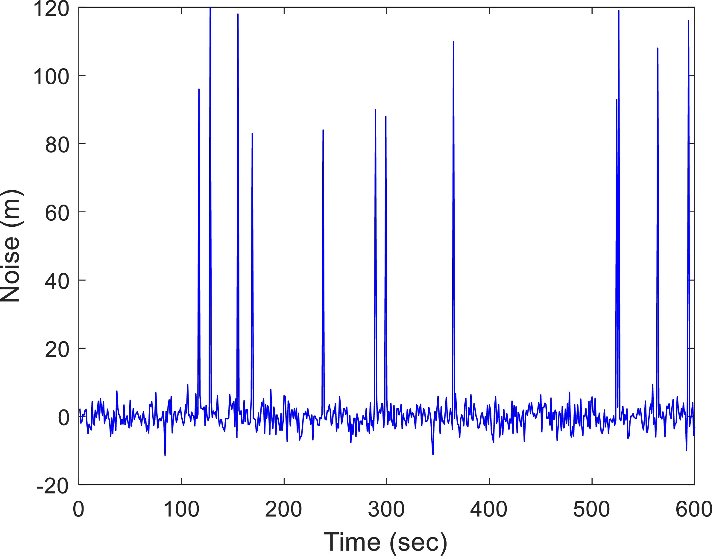
To evaluate filter robustness against large-magnitude outliers, the first simulation scenario considers impulsive measurement disturbances. Unlike Gaussian noise, impulse noise contains sporadic large deviations that occur with low probability but can substantially degrade positioning accuracy. Such disturbances are particularly challenging for MMSE-based filters, since the squared-error formulation magnifies the influence of large residuals. In this study, the pseudorange measurement error is modelled using a contaminated noise model with a low-probability impulsive component:
 $${r_k}\sim 0.9{\rm{8}}{\mkern 1mu} N(0,{\rm{4}}) \cup 0.0{\rm{2}}{\mkern 1mu} {\rm{U[80,120]}}$$
This formulation assigns a 98% probability to nominal Gaussian noise and a 2% probability to impulsive disturbances uniformly distributed over the interval [80, 120] m, thereby simulating occasional large-magnitude outliers. The resulting noise sequence is illustrated in Figure 6.
Time history of pseudorange observable error under impulsive noise conditions.

Monte Carlo simulations under multiple non-Gaussian noise scenarios were conducted to evaluate positioning performance in the east, north and altitude directions using RMSE as the metric. Figures 7 and 8 present the positioning errors and RMSE comparisons under impulsive noise conditions for two groups of filters. For clarity, Figure 7 compares the kernel-based information-theoretic methods, namely MEE-EKF, MCC-EKF and CEE-EKF, while Figure 8 compares ST-EKF, VB-EKF and CEE-EKF as representative robust and adaptive methods. The results show that CEE-EKF consistently achieves smaller positioning errors and lower RMSE values than the competing methods, demonstrating the best overall robustness under impulsive noise conditions.
Comparison of positioning errors and RMSE for EKF, MEE-EKF, MCC-EKF and CEE-EKF under impulsive noise conditions.

Comparison of positioning errors and RMSE for EKF, ST-EKF, VB-EKF and CEE-EKF under impulsive noise conditions.

Figure 8 Long description
The image contains six line graphs comparing positioning errors and RMSE for different filtering methods under impulsive noise conditions. Panel A: A line graph showing East Error over time in seconds. The y-axis represents East Error in meters, and the x-axis represents Time in seconds. Panel B: A line graph showing North Error over time in seconds. The y-axis represents North Error in meters, and the x-axis represents Time in seconds. Panel C: A line graph showing Altitude Error over time in seconds. The y-axis represents Altitude Error in meters, and the x-axis represents Time in seconds. Panel D: A line graph showing East RMSE over time in seconds. The y-axis represents East RMSE in meters, and the x-axis represents Time in seconds. Panel E: A line graph showing North RMSE over time in seconds. The y-axis represents North RMSE in meters, and the x-axis represents Time in seconds. Panel F: A line graph showing Altitude RMSE over time in seconds. The y-axis represents Altitude RMSE in meters, and the x-axis represents Time in seconds. Each graph includes four lines representing different filtering methods: EKF, ST-EKF, VB-EKF, and CEE-EKF. The lines show the performance of each method over time, with visible trends and variations in error and RMSE values.
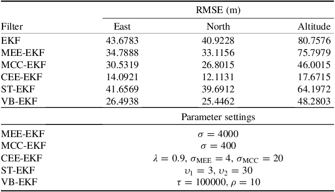
Table 1 summarises the RMSE results of the six filters under impulsive noise conditions, along with the corresponding parameter settings for each method. Since the evaluated filters are based on different robustness mechanisms, their parameters serve different purposes and are not directly comparable in magnitude. For the ST-EKF,
 ${\upsilon _{\rm{1}}}$
and
 ${\upsilon _{\rm{2}}}$
denote the degrees-of-freedom parameters of the Student’s t distribution, which control the heaviness of the distribution tails and thereby determine the filter’s robustness to impulsive disturbances. For VB-EKF,
 $\tau $
and
 $\rho $
are associated with the variational Bayesian inference mechanism and affect the adaptive estimation of measurement noise statistics.
RMSE comparison of six filters under impulse noise conditions.

Table 1. Long description
A table comparing RMSE values of six filters under impulse noise conditions. The table has 7 rows and 4 columns. The columns are labeled Filter, East, North, and Altitude. The row labels are EKF, MEE-EKF, MCC-EKF, CEE-EKF, ST-EKF, and VB-EKF. The table also includes parameter settings for each filter. Row 1: EKF, East, 43.6783, North, 40.9228, Altitude, 80.7576. Row 2: MEE-EKF, East, 34.7888, North, 33.1156, Altitude, 75.7979. Row 3: MCC-EKF, East, 30.5319, North, 26.8015, Altitude, 46.0015. Row 4: CEE-EKF, East, 14.0921, North, 12.1131, Altitude, 17.6715. Row 5: ST-EKF, East, 41.6569, North, 39.6912, Altitude, 64.1972. Row 6: VB-EKF, East, 26.4938, North, 25.4462, Altitude, 48.2803. Parameter settings: MEE-EKF, sigma equals 4000. MCC-EKF, sigma equals 400. CEE-EKF, sigma subscript MEE equals 4, sigma subscript MCC equals 20. ST-EKF, nu subscript 1 equals 3, nu subscript 2 equals 30. VB-EKF, tau equals 100000, rho equals 10.
The selection of kernel bandwidths for MEE-EKF, MCC-EKF and CEE-EKF is guided by the scale and structure of the residuals in each formulation. In MEE-EKF, the kernel is applied to pairwise residual differences, which may span a wide range under non-Gaussian noise conditions; therefore, a larger bandwidth is required to ensure a smooth and stable estimate of the error distribution. In MCC-EKF, the kernel is applied directly to individual residuals, so moderate bandwidth values are sufficient to achieve a balance between sensitivity and robustness. In CEE-EKF, the cost function incorporates both correntropy-based and entropy-based terms, in which the residuals appear in both individual and pairwise forms. The weighting coefficient λ regulates the trade-off between the correntropy-based and entropy-based terms in the cost function. A value of
 $\lambda {\rm{ = 0}}{\rm{.9}}$
is adopted to emphasise correntropy-based local robustness while retaining the entropy-based term for global distribution shaping and ensuring convergence stability.
Unlike MEE-EKF and MCC-EKF which each use a single kernel, CEE-EKF employs two kernel parameters,
 ${\sigma _{{\rm{MEE}}}}$
and
 ${\sigma _{{\rm{MCC}}}}$
, to separately control the entropy-based and correntropy-based components of the cost function. Because of this combined structure, different bandwidths are used to control both local robustness and global error-distribution characteristics. Accordingly, these kernel parameters enhance robustness to large deviations while maintaining sensitivity to nominal measurements. The kernel bandwidths are further tuned according to the noise level of each experiment: larger values are used in the simulation experiments, where non-Gaussian disturbances yield residuals with significantly higher magnitudes, while smaller values are adopted in the field test, where the measurement noise is relatively mild. As summarised in Table 1, the CEE-EKF attains the lowest RMSE across all three coordinate directions, with the most significant improvement observed in the altitude component.
(2) Scenario 2: GPS observables affected by Gaussian mixture noise conditions.
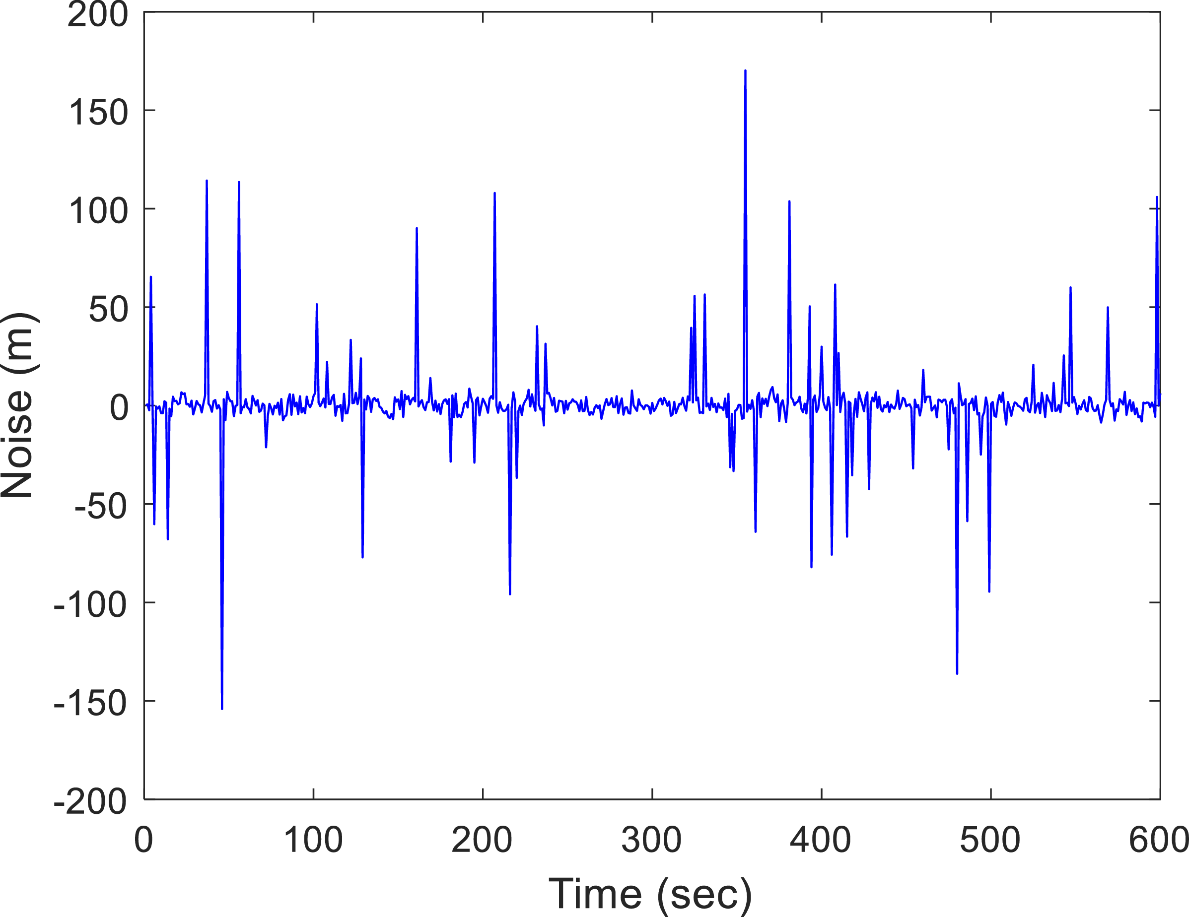
In practical GPS applications, measurement noise rarely follows a single Gaussian distribution. To better represent real-world non-Gaussian conditions, a mixed Gaussian noise model is adopted in this study, consisting of a dominant low-variance Gaussian component and a secondary high-variance Gaussian component. The measurement noise is modelled as follows:
 $${r_k} \sim 0.9N(0,10{\rm{0}}) \cup 0.{\rm{1}}N{\rm{(0,1}}{{\rm{0}}^7}{\rm{)}}$$
This model assigns a 90% occurrence probability to the low-variance component and a 10% occurrence probability to the high-variance component, thereby capturing a non-Gaussian error distribution. The corresponding noise sequence is shown in Figure 9.
Time history of pseudorange observable error under Gaussian mixture noise conditions.

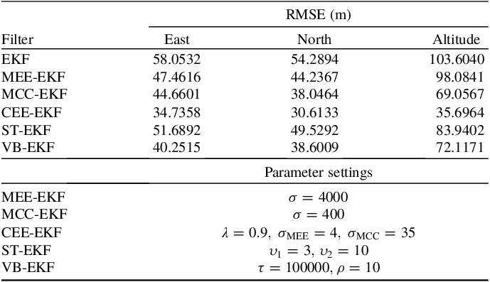
Table 2 summarises the parameter settings adopted for each filter in the Gaussian mixture noise scenario. The parameter definitions and their functional roles are the same as those described for Table 1, but the numerical values were re-adjusted to account for the different statistical characteristics of the noise environment. Since Gaussian mixture noise differs from impulse noise in both error distribution structure and variability, scenario-dependent parameter tuning was necessary to provide stable and representative performance for each method. To maintain fairness, all compared filters were tuned according to the same principle under the corresponding noise condition. As summarised in Table 2, CEE-EKF again achieves the lowest RMSE in all three directions, with the most pronounced advantage observed in the altitude component.
RMSE comparison of six filters under Gaussian mixture noise conditions.

Table 2. Long description
A table comparing RMSE values for different filters under Gaussian mixture noise conditions. The table has 7 rows and 4 columns. The columns are labeled Filter, East, North, and Altitude. The row labels are EKF, MEE-EKF, MCC-EKF, CEE-EKF, ST-EKF, and VB-EKF. The values in the East column are 58.0532, 47.4616, 44.6601, 34.7358, 51.6892, and 40.2515. The values in the North column are 54.2894, 44.2367, 38.0464, 30.6133, 49.5292, and 38.6009. The values in the Altitude column are 103.6040, 98.0841, 69.0567, 35.6964, 83.9402, and 72.1171. The table also includes parameter settings for each filter.
Figures 10 and 11 present the positioning errors and RMSE comparisons under Gaussian mixture noise conditions for two groups of filters classified according to their algorithmic characteristics. Figure 10 compares MEE-EKF, MCC-EKF and CEE-EKF as kernel-based information-theoretic robust filtering methods, whereas Figure 11 compares ST-EKF, VB-EKF and CEE-EKF as other alternative robust and adaptive estimation approaches. The results show that CEE-EKF consistently yields smaller positioning errors and lower RMSE values than the competing methods in both groups. Although ST-EKF, VB-EKF, MEE-EKF and MCC-EKF each improve estimation performance to some extent, CEE-EKF remains the most stable in the east, north and altitude directions, with the most pronounced advantage observed in the altitude component.
Comparison of positioning errors and RMSE for EKF, MEE-EKF, MCC-EKF and CEE-EKF under Gaussian mixture noise conditions.

Figure 10 Long description
The image contains six line graphs comparing positioning errors and RMSE for EKF, MEE-EKF, MCC-EKF, and CEE-EKF under Gaussian mixture noise conditions. Panel A: East Error. The line graph shows East Error in meters over time in seconds. The legend indicates four methods: EKF (black dashed line), MEE-EKF (green line), MCC-EKF (red line), and CEE-EKF (blue line). Panel B: North Error. The line graph shows North Error in meters over time in seconds. The legend is the same as in Panel A. Panel C: Altitude Error. The line graph shows Altitude Error in meters over time in seconds. The legend is the same as in Panel A. Panel D: East RMSE. The line graph shows East RMSE in meters over time in seconds. The legend is the same as in Panel A. Panel E: North RMSE. The line graph shows North RMSE in meters over time in seconds. The legend is the same as in Panel A. Panel F: Altitude RMSE. The line graph shows Altitude RMSE in meters over time in seconds. The legend is the same as in Panel A.
Comparison of positioning errors and RMSEs for EKF, ST-EKF, VB-EKF and CEE-EKF under Gaussian mixture noise conditions.

6.2. Validation through field test data
To further assess the robustness of the filter, an offline simulation based on real-world data is performed for additional validation. A data-driven simulation, implemented within a software-in-the-loop (SIL) framework, is used to introduce an additional pseudorange error sequence into the field measurements. To demonstrate the practical applicability of the proposed CEE-EKF, field experiments were conducted at the sports field of National Taiwan Ocean University in Taiwan (25.150°N, 121.773°E). The site provides realistic outdoor GNSS conditions, where nearby buildings and surrounding structures induce multipath effects, partial signal blockage and occasional NLOS reception.
Real-world data were collected using a dual-receiver configuration consisting of a NovAtel receiver for pseudorange observations and a u-blox RTK (Real-Time Kinematic) receiver operating in RTK mode to provide centimetre-level reference trajectories. The NovAtel unit provided raw pseudorange measurements at 1 Hz, which were used as the input to all filtering algorithms. Both receivers were rigidly mounted together to ensure spatial and temporal alignment. Data were collected by walking along predefined trajectories within the sports field, covering a range of GNSS conditions, including multipath-affected and NLOS regions, partially obstructed areas, and open-sky environments. To further evaluate the robustness of the proposed filter under controlled impulsive disturbances, an additional pseudorange error sequence was superimposed on the real NovAtel measurements according to the following model:
 $${r_k} \sim 0.9{\rm{8}}{\mkern 1mu} {\delta _0} \cup 0.0{\rm{2}}{\mkern 1mu} {s_k}{\rm{U[1}},100{\rm{]}}$$
where
 ${\mkern 1mu} {\delta _0}$
denotes a point mass at zero, indicating that no additional error is injected at the corresponding epoch. Since the real GPS measurements already contain receiver noise and environmental interference, no additional background Gaussian noise was added. The variable
 ${s_k} \in \{ - 1, + 1\} $
is an equally probable random sign. When an impulsive error occurs, it is applied to one randomly selected satellite pseudorange at that epoch. The 2% outlier probability is kept the same as that in Scenario 1 (Eq. 98), whereas the amplitude range is reduced to account for the smaller error scale in the field-test environment.
Figure 13 shows the estimated trajectories produced by all six filters overlaid on satellite imagery of the test site, enabling a direct geographic comparison with the reference route under field conditions with injected impulsive pseudorange disturbances. The EKF and ST-EKF exhibit the largest deviations from the reference trajectory, particularly in segments affected by measurement degradation. The MEE-EKF and MCC-EKF show moderate improvements, while the VB-EKF tracks the reference path more closely. Among all methods, the CEE-EKF maintains the closest agreement with the reference trajectory throughout the route, demonstrating stronger suppression of outlier-induced divergence. Figure 14 further presents the corresponding trajectory estimates in the East-North coordinate frame, where lateral deviations among the filters are more clearly visible and the same performance trend is consistently observed.
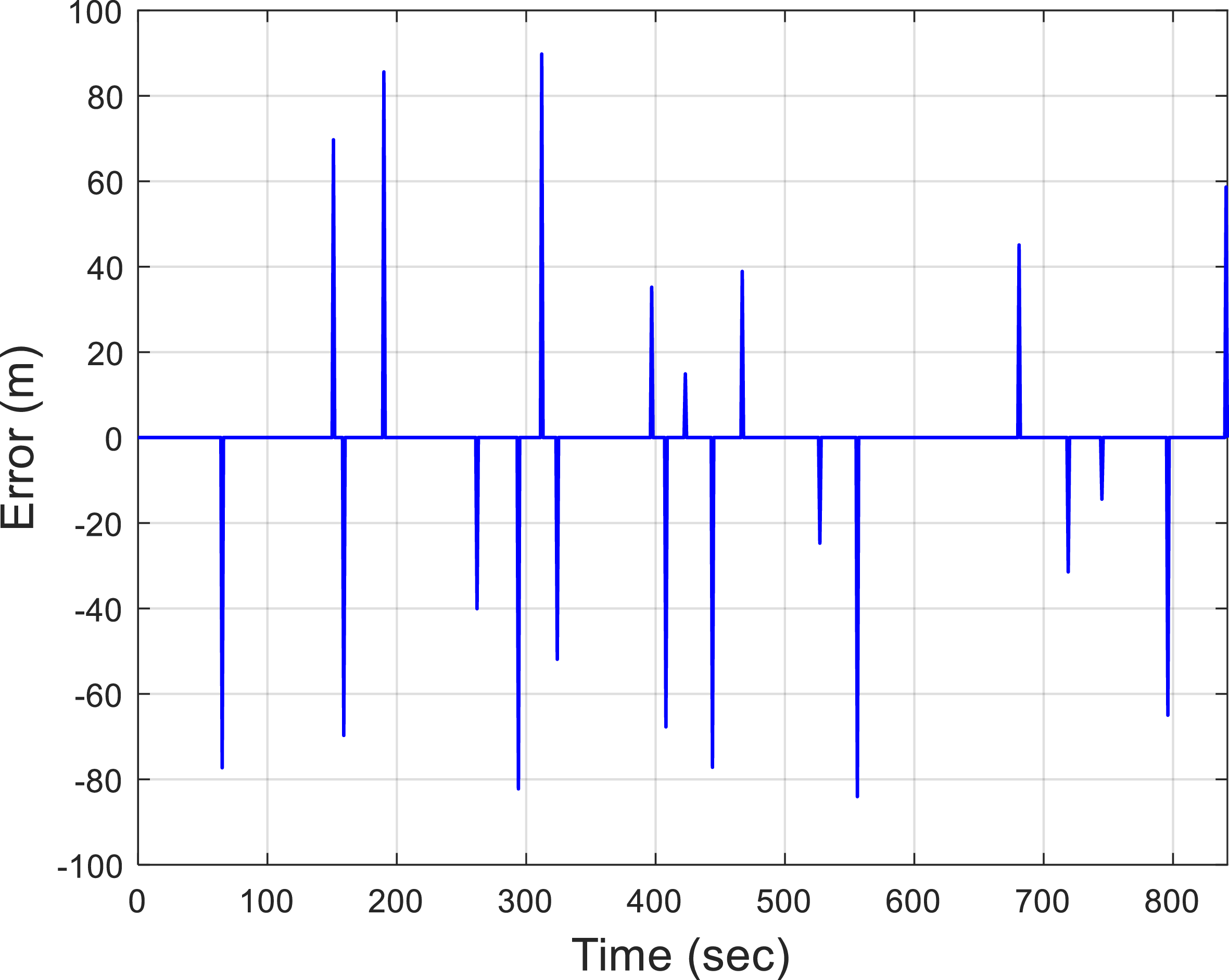
Injected GPS pseudorange error used in the field test.

Field-test trajectory and state estimates based on six filters: EKF, MEE-EKF, MCC-EKF, ST-EKF, VB-EKF and CEE-EKF, under impulsive noise conditions.

Figure 13 Long description
Aerial view of a stadium with various trajectory paths overlaid. The image shows different paths taken by six filters: EKF, MEE-EKF, MCC-EKF, ST-EKF, VB-EKF, and CEE-EKF. The paths are color-coded and labeled accordingly. The stadium is surrounded by various structures and fields. The trajectories are plotted on a map with latitude and longitude coordinates ranging from 25°09'04''N to 25°09'00''N and 121°46'38''E to 121°46'46''E.
Comparison of positioning results for various filters under impulsive pseudorange noise.

Figure 15 shows the positioning errors of two groups of filters along the field trajectory. For clarity, the methods are categorised based on their algorithmic characteristics. Figures 15a–c compare EKF, MEE-EKF, MCC-EKF and CEE-EKF, whereas Figures 15d–f present a comparison of EKF, ST-EKF, VB-EKF and CEE-EKF. In both groups, EKF shows the largest error spikes, while the other robust filters provide different levels of improvement. CEE-EKF consistently yields the smallest positioning errors in the east, north and altitude directions.
Comparison of positioning errors of two filter groups under real-world impulsive noise conditions: (a)–(c) EKF, MEE-EKF, MCC-EKF and CEE-EKF; (d)–(f) EKF, ST-EKF, VB-EKF and CEE-EKF.

Figure 15 Long description
The image contains six line graphs comparing positioning errors of different filters under real-world impulsive noise conditions. Panel A: A line graph showing East positioning errors over time (seconds) for EKF, MEE-EKF, MCC-EKF, and CEE-EKF. Panel B: A line graph showing North positioning errors over time (seconds) for EKF, MEE-EKF, MCC-EKF, and CEE-EKF. Panel C: A line graph showing Altitude positioning errors over time (seconds) for EKF, MEE-EKF, MCC-EKF, and CEE-EKF. Panel D: A line graph showing East positioning errors over time (seconds) for EKF, ST-EKF, VB-EKF, and CEE-EKF. Panel E: A line graph showing North positioning errors over time (seconds) for EKF, ST-EKF, VB-EKF, and CEE-EKF. Panel F: A line graph showing Altitude positioning errors over time (seconds) for EKF, ST-EKF, VB-EKF, and CEE-EKF. Each graph has time (seconds) on the x-axis and positioning error (meters) on the y-axis. The graphs show different trends and patterns for each filter type.
Figure 16 illustrates the number of visible satellites and the positioning errors observed during the field test for two groups of filters. Specifically, Figure 16a compares MEE-EKF, MCC-EKF and CEE-EKF, while Figure 16b presents a comparison of ST-EKF, VB-EKF and CEE-EKF. In both groups, reductions in visible satellite count are generally accompanied by increased positioning errors, reflecting the impact of degraded measurement conditions. Compared with the other methods, CEE-EKF maintains smaller error variations and more stable estimation performance throughout the trajectory, further confirming its stronger adaptability in field environments.
Number of visible satellites and positioning errors during field testing: (a) comparison of MEE-EKF, MCC-EKF and CEE-EKF; (b) comparison of ST-EKF, VB-EK, and CEE-EKF.

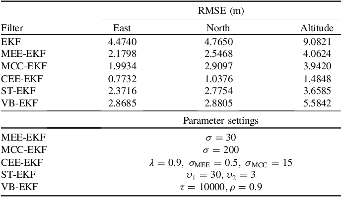
Table 3 summarises the RMSE results of the six filters in the field experiments, together with their corresponding parameter settings. As shown in the table, the CEE-EKF achieves the lowest RMSE in the east, north and altitude components, with the largest improvement observed in the altitude direction. This result indicates that the CEE-EKF maintains better positioning stability under field-test conditions with injected impulsive pseudorange disturbances. The kernel parameters listed in Table 3 should be interpreted according to their roles in the corresponding objective functions. In the MEE-EKF, the kernel is applied to pairwise residual differences, so a relatively large bandwidth is required to maintain a stable entropy estimate. In the MCC-EKF, the kernel is applied directly to individual residuals and its bandwidth determines how strongly large pseudorange residuals are attenuated. In the CEE-EKF, two kernel parameters are used for the correntropy-based and entropy-based terms, respectively. This allows the filter to balance local residual suppression and overall error-distribution shaping, while still maintaining stable performance with smaller kernel values in the field-test case.
RMSE comparison of six filters under field test conditions and corresponding parameter settings.

Table 3. Long description
A table comparing RMSE values for different filters in field tests. The table has 7 rows and 4 columns. The columns are labeled Filter, East, North, and Altitude. The row labels are EKF, MEE-EKF, MCC-EKF, CEE-EKF, ST-EKF, and VB-EKF. The RMSE values for each filter in the East, North, and Altitude columns are as follows: Row 1: EKF, 4.4740, 4.7650, 9.0821. Row 2: MEE-EKF, 2.1798, 2.5468, 4.0624. Row 3: MCC-EKF, 1.9934, 2.9097, 3.9420. Row 4: CEE-EKF, 0.7732, 1.0376, 1.4848. Row 5: ST-EKF, 2.3716, 2.7754, 3.6585. Row 6: VB-EKF, 2.8685, 2.8805, 5.5842. The table also includes parameter settings for each filter: MEE-EKF, sigma equals 30. MCC-EKF, sigma equals 200. CEE-EKF, sigma sub MEE equals 0.5, sigma sub MCC equals 15. ST-EKF, nu sub 1 equals 30, nu sub 2 equals 3. VB-EKF, tau equals 10000, rho equals 0.9.
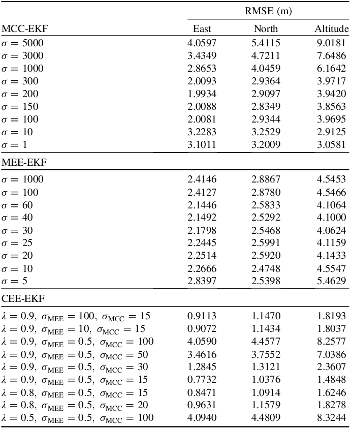
To examine the effect of parameter selection, Table 4 compares different parameter settings for the MCC-EKF, MEE-EKF and CEE-EKF under field-test conditions. The results show that the MEE-EKF and MCC-EKF are sensitive to bandwidth selection. A large bandwidth weakens the robust filtering effect and makes the filter behaviour closer to that of the standard EKF, whereas an excessively small bandwidth may cause numerical instability or a substantial increase in estimation error. Therefore, careful bandwidth selection is necessary for these single-kernel methods. By contrast, the CEE-EKF benefits from the combined use of correntropy-based and entropy-based terms. The two kernel parameters work together to suppress large residuals and maintain the overall error-distribution structure, allowing the filter to achieve stable outlier suppression over a narrower parameter range. Adaptive online tuning of these parameters remains an important issue for future research.
Effect of parameter settings on filter performance evaluated in terms of RMSE under field test conditions.

Table 4. Long description
A table comparing the performance of MCC-EKF, MEE-EKF, and CEE-EKF filters under field test conditions. The table has 21 rows and 4 columns. The columns are labeled East, North, and Altitude with RMSE values in meters. The rows are grouped by filter types and parameter settings. For MCC-EKF, the parameter sigma varies from 5000 to 1. For MEE-EKF, sigma varies from 1000 to 5. For CEE-EKF, lambda and sigma values vary with different combinations. Each row lists the RMSE values for East, North, and Altitude corresponding to specific parameter settings.
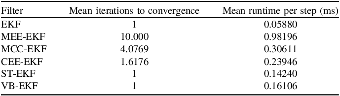
Table 5 summarises the mean number of fixed-point iterations and the mean per-step runtime for each filter, measured over all Monte Carlo runs under the impulse noise scenario. EKF, ST-EKF and VB-EKF are non-iterative methods and complete each update in a single pass, with runtimes below 0.2 ms. Among the fixed-point-based filters, MEE-EKF reaches the preset iteration limit of 10 iterations per step under severe impulsive noise. This behaviour is mainly related to its pairwise residual interactions and full kernel evaluations in the minimum error entropy update. By contrast, MCC-EKF and CEE-EKF require only 4.0769 and 1.6176 iterations on average, respectively. In terms of runtime, MEE-EKF has the highest computational cost (0.98196 ms), whereas MCC-EKF and CEE-EKF require 0.30611 ms and 0.23946 ms per step, respectively. These results show that CEE-EKF maintains a relatively low computational burden while achieving improved estimation accuracy.
Average number of iterations and mean per-step runtime for each filter under the impulse noise scenario.

Table 5. Long description
A table comparing mean iterations to convergence and mean runtime per step for different filters. The table has three columns: Filter, Mean iterations to convergence, and Mean runtime per step (ms). It has six rows corresponding to different filters: EKF, MEE-EKF, MCC-EKF, CEE-EKF, ST-EKF, and VB-EKF. Row 1: EKF, 1, 0.05880. Row 2: MEE-EKF, 10.000, 0.98196. Row 3: MCC-EKF, 4.0769, 0.30611. Row 4: CEE-EKF, 1.6176, 0.23946. Row 5: ST-EKF, 1, 0.14240. Row 6: VB-EKF, 1, 0.16106.
7. Conclusions and future work
This paper investigates the GPS navigation state estimation problem under non-Gaussian noise conditions through a comparative evaluation of the proposed CEE-EKF against five benchmark methods, namely EKF, MEE-EKF, MCC-EKF, ST-EKF and VB-EKF. The comparison is conducted under two simulation scenarios, including impulsive noise and Gaussian mixture noise, as well as real-world field tests with additional disturbances injected into the pseudorange observables, to assess robustness and estimation accuracy in both simulated and practical non-Gaussian environments.
This work provides a systematic benchmarking of six EKF variants spanning classical, information-theoretic, robust and adaptive paradigms within a unified GPS positioning framework, offering a comprehensive reference for filter selection in non-Gaussian navigation applications. Furthermore, the CEE-EKF is specifically formulated and evaluated within the GPS pseudorange observation model, demonstrating its effectiveness for satellite-based positioning under various non-Gaussian noise conditions, including impulsive and Gaussian mixture noise. Moreover, the simulation results are further validated through real-world field experiments using u-blox and NovAtel receivers, providing empirical evidence of the proposed approach under practical operating conditions.
The results consistently show that the CEE-EKF achieves the best overall performance among the compared methods. It provides superior suppression of impulsive outliers, maintains stable state estimation and shows the closest agreement with the RTK reference trajectory in field tests. Across all scenarios with complex non-Gaussian disturbances, the CEE-EKF achieves the lowest RMSE in the east, north and altitude components. These findings confirm that integrating minimum error entropy and maximum correntropy within a unified framework yields a more effective filtering strategy than either criterion alone, and further demonstrate the suitability of the CEE-EKF for robust GPS navigation in realistic, disturbance-prone environments. In addition, the results highlight that well-chosen parameter settings improve both stability and accuracy across all coordinate components, emphasising the importance of careful calibration or adaptive tuning in practical applications.
Adaptive online tuning of these parameters remains an important direction for future research. In future work, we plan to address this problem by developing an online adaptive strategy for key filter parameters, such as the kernel bandwidth and the weighting coefficient between the MEE and MCC terms. This will aim to improve generalisation under varying noise conditions and enhance the applicability of the CEE-EKF framework to more demanding real-time navigation scenarios.
Acknowledgement
The authors gratefully acknowledge the support of the National Science and Technology Council, Taiwan under grant numbers NSTC 111-2221-E-019-047 and NSTC 112-2221-E-019-030.