1. Introduction
Inertial waves are ubiquitous in rotating fluids. They are associated with the Coriolis restoring force. They propagate at a fixed angle
 $\pi /2-\theta _c$
relative to the rotation axis that only depends on the inertial wave frequency
 $\omega ^*$
through the dispersion relation
 $\omega ^*= 2 \Omega ^* \cos \theta _c$
(
 $\Omega ^*$
being the rotation rate) (Greenspan Reference Greenspan1968). This angle is conserved when waves reflect on boundaries. Owing to this property, the width of an inertial wave beam contracts or expands, depending on the inclination of the boundary relative to the propagation angle
 $\theta _c$
and the rotation axis (Phillips Reference Phillips1963; Le Dizès Reference Le Dizès2020). The contraction effect is responsible for the creation of inviscid singularities on the critical characteristics, such as the tangent lines from the critical points on a convex boundary (Le Dizès Reference Le Dizès2024), and the attractors inside a bounded domain (Ogilvie Reference Ogilvie2020). Inviscid singularities can be understood as the outcome of the hyperbolic character of the Poincaré equation, namely, the ability to transport singularities (Kerswell Reference Kerswell1995) and to form an ill-posed Cauchy problem in closed domains (Rieutord, Georgeot & Valdettaro Reference Rieutord, Georgeot and Valdettaro2000).
In numerical simulations and experiments, these inviscid singularities are smoothed out by viscosity, giving rise to oscillatory internal shear layers around the critical characteristics (Kerswell Reference Kerswell1995). These layers become the dominant feature of a global viscous solution when inviscid singularities are present. The internal shear layers associated with a critical slope singularity have been experimentally observed in both rotating (Greenspan Reference Greenspan1968) and stratified (Mowbray & Rarity Reference Mowbray and Rarity1967; Zhang, King & Swinney Reference Zhang, King and Swinney2007) fluids, owing to the similarity between the dispersion relation of inertial waves and that of internal gravity waves. Similarly, in a bounded domain, attractors give rise to internal shear layers that have been observed in various configurations (Maas et al. Reference Maas, Benielli, Sommeria and Lam1997; Hazewinkel et al. Reference Hazewinkel, Van Breevoort, Dalziel and Maas2008; Klein et al. Reference Klein, Seelig, Kurgansky and Ghasemi2014).
The mathematical description of the internal oscillatory shear layers relies on local asymptotic analysis in the limit of the small Ekman number
 $E$
(defined as the ratio between the viscous term and the Coriolis term, see below). Although different scalings have been identified for the width of these layers in forced and eigenvalue problems, including
 $E^{1/3}$
,
 $E^{1/4}$
,
 $E^{1/5}$
and
 $E^{1/6}$
(Kerswell Reference Kerswell1995; Rieutord & Valdettaro Reference Rieutord and Valdettaro2018), the scaling in
 $E^{1/3}$
appears as the natural scaling in a forced problem for the width of the internal shear layer associated with a critical slope singularity or an attractor. For the former, the scaling was derived by dominant balance (Walton Reference Walton1975a
,Reference Walton
b
; Kerswell Reference Kerswell1995), and numerically validated (Lin & Noir Reference Lin and Noir2021). For the latter, it was inferred by Ogilvie (Reference Ogilvie2005) and numerically validated by Grisouard, Staquet & Pairaud (Reference Grisouard, Staquet and Pairaud2008).
The viscous structure of these layers has been the subject of many works. The first theoretical work in an oscillatory context goes probably back to Walton (Reference Walton1975a
). The building block is now believed to be a class of similarity solutions that was introduced by Moore & Saffman (Reference Moore and Saffman1969) in rotating fluids and Thomas & Stevenson (Reference Thomas and Stevenson1972) in stratified fluids. These solutions depend on an index
 $m$
that is related to the strength of the underlying inviscid singularity (Le Dizès Reference Le Dizès2024). The similarity solutions were initially used to describe in the far field the solution generated by a localised oscillating source (Hurley & Keady Reference Hurley and Keady1997; Voisin Reference Voisin2003). In this context, Machicoane et al. (Reference Machicoane, Cortet, Voisin and Moisy2015) have shown that the index
 $m$
is linked to multipolar character of the source. Tilgner (Reference Tilgner2000) and Le Dizès (Reference Le Dizès2015) have also shown that they describe the thin shear layers generated from the border of an oscillating disk. The use of the similarity solutions to describe the oscillatory internal shear layers generated from a critical point was first made by Le Dizès & Le Bars (Reference Le Dizès and Le Bars2017) in the case of a viscous forcing for a librating object in an unbounded domain. He et al. (Reference He, Favier, Rieutord and Le Dizès2022, Reference He, Favier, Rieutord and Le Dizès2023) extended these results to a bounded geometry for both a periodic wave pattern and an attractor. For the attractor case, they used original ideas that were introduced in an inclined rotating square subject to a body forcing by Ogilvie (Reference Ogilvie2005). These ideas will also be used in the present study.
In our previous works (Le Dizès & Le Bars Reference Le Dizès and Le Bars2017; He et al. Reference He, Favier, Rieutord and Le Dizès2022, Reference He, Favier, Rieutord and Le Dizès2023), the internal shear layers were generated by libration, that is, by a viscous forcing at the critical point. In the present study, we consider an inviscid forcing, specifically vertical oscillation, where internal shear layers are forced through pressure coupling. For such a forcing, the nature of the internal shear layers generated from a critical point is expected to be different. Le Dizès (Reference Le Dizès2024) has explained that, in contrast to the viscous case, the amplitude of the internal shear layer cannot be obtained in closed form from a local analysis of the critical point. Our analysis will therefore go through the derivation of global inviscid solutions before considering internal shear layers. It will be limited to two-dimensional geometries.
We start with the classical problem of an oscillating cylinder in an unbounded domain. The inviscid problem has been solved in a stratified fluid by Hurley (Reference Hurley1997). We provide here the inviscid solution in a rotating fluid using the same approach. This solution is singular along the characteristics issued from the critical points. From the behaviour of the solution close to the singularity, we obtain the index and the amplitude of the similarity solution that describes the viscous structure of the internal shear layer. An alternative method based on a global viscous solution is also given in Appendix B. The approximation that is obtained is compared with viscous numerical results obtained for very small Ekman numbers. We then consider the cylindrical shell geometry. The ray patterns strongly depend on the frequency. For a frequency
 $\omega ^*= \sqrt {2}\,\Omega ^*$
, the propagation is at 45 degrees with respect to the rotation axis. We first consider this case, for which the ray trajectories are periodic. A global inviscid solution is obtained by writing down the conditions of reflection on each trajectory. This solution is singular on the critical lines. To obtain an approximation valid close to these lines, we adapt the method used in He et al. (Reference He, Favier, Rieutord and Le Dizès2022) for a viscous forcing. Both the index and the amplitude of the similarity solutions needed to build this asymptotic solution are obtained by matching this solution with the global inviscid solution. Again, the theoretical results are compared with numerical results. In the last section, we consider the case of an attractor. An asymptotic solution is obtained close to the attractor using the analysis developed in He et al. (Reference He, Favier, Rieutord and Le Dizès2023), and then compared with numerical results. Additional numerical results for particular attractors for which there is no asymptotic theory are also provided in Appendix D. The paper is concluded by summarising the main results, emphasising the difference between inviscid and viscous forcings, and discussing the applicability of the results in a three-dimensional context.
2. Framework
2.1. Geometry and governing equations
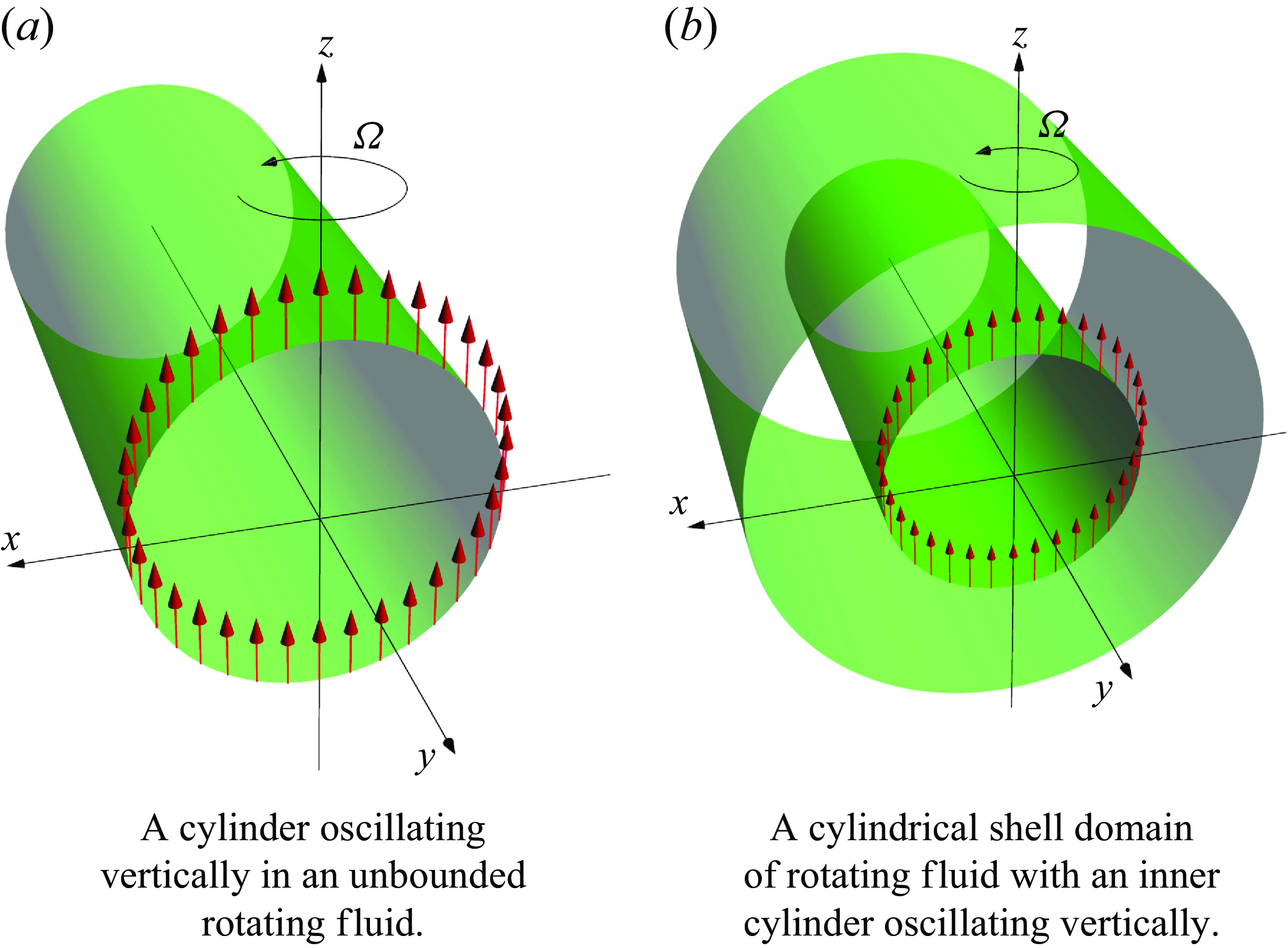
We consider the internal shear layers generated by a two-dimensional cylindrical body oscillating vertically in either an unbounded or bounded domain. For the former, the configuration is a circular cylinder immersed in an unbounded fluid, as shown in figure 1(a); for the latter, the geometry is a cylindrical annulus, as shown in figure 1(b). In both cases, the cylinders’ axes are horizontal and extend to infinity, making the problems two-dimensional. We adopt a Cartesian coordinate system, where the axis
 $Oz$
is vertical to the horizontal plane
 $Oxy$
. The cylinders’ axes are along the axis
 $Oy$
such that cross-sections lie in the vertical plane
 $Oxz$
. The flow is that of an incompressible fluid with constant kinematic viscosity
 $\nu ^*$
, rotating around the axis
 $Oz$
with a uniform rotation rate
 $\Omega ^*$
. Although the flow field only depends on
 $x$
and
 $z$
, it has three velocity components.
Due to the two-dimensional nature of the problem, we can use a polar coordinate system to describe the flow field, with the radial coordinate
 $\varrho =\sqrt {x^2+z^2}$
and angular coordinate
 $\vartheta =\arctan {(z/x)}$
. The flow domain is defined by
 $\varrho \in [\varrho _i^*, \varrho _o^*]$
, where
 $\varrho _o^*$
is infinite for the unbounded case. In the bounded case, we write
 $[\varrho _i^*, \varrho _o^*]=[\eta \varrho ^*,\varrho ^*]$
, with
 $\eta \in ]0,1[$
defining the aspect ratio. For convenience of comparison, the radial range of the unbounded domain is chosen as
 $[\varrho _i^*, \varrho _o^*]=[\eta \varrho ^*,+\infty ]$
, with the same inner radius as the bounded domain.
Two-dimensional configurations in unbounded
 $(a)$
and bounded
 $(b)$
domains.

For both configurations, lengths are non-dimensionalised by
 $\varrho ^*$
, resulting in non-dimensional radial ranges of
 $[\eta ,1]$
for the bounded domain and
 $[\eta ,+\infty ]$
for the unbounded domain. Thus, the non-dimensional radius of the forced cylinder is
 $\eta$
in both cases. This choice of non-dimensionalisation is made to facilitate the comparison between inviscid results in unbounded and bounded domains. Time is non-dimensionalised by the angular period
 $1/\Omega ^*$
. Using these scales, the Ekman number is defined as
 \begin{align} E=\frac {\nu ^*}{\Omega ^*\varrho ^{*2}}. \end{align}
The imposed harmonic forcing is the vertical oscillation of the cylinder in the unbounded domain or the inner cylinder in the bounded domain (see red arrows in figure 1), with the displacement amplitude
 $\varepsilon =\varepsilon ^*/\varrho ^*$
(
 $\varepsilon \ll 1$
) and the frequency
 $\omega =\omega ^*/\Omega ^*$
. As in our previous works (Le Dizès & Le Bars Reference Le Dizès and Le Bars2017; He et al. Reference He, Favier, Rieutord and Le Dizès2022, Reference He, Favier, Rieutord and Le Dizès2023), we focus on the linear harmonic response and consider solutions in the form
 \begin{align} (\boldsymbol{v},p)\textrm{e}^{-\textrm{i}\omega t}+c.c., \end{align}
where
 $c.c.$
denotes the complex conjugate. The velocity
 $\boldsymbol{v}$
and pressure
 $p$
satisfy the linearised incompressible Navier–Stokes equations in the rotating frame
 \begin{align}& -\textrm{i}\omega v_x-2v_y+\frac {\partial p}{\partial x}-E\nabla ^2v_x=0, \end{align}
 \begin{align}&\quad\, -\textrm{i}\omega v_z+\frac {\partial p}{\partial z}-E\nabla ^2v_z=0, \end{align}
 \begin{align}& -\textrm{i}\omega v_y+2v_x-E\nabla ^2v_y=0, \end{align}
 \begin{align}&\qquad\quad \frac {\partial v_x}{\partial x}+\frac {\partial v_z}{\partial z}=0, \end{align}
with the Laplacian operator
 \begin{align} \nabla ^2=\partial ^2/\partial x^2+\partial ^2/\partial z^2. \end{align}
As the oscillations are assumed to be very small (
 $\varepsilon \ll 1$
), the (inner) cylinder can be assumed fixed at leading order. The boundary conditions at the surface of the (inner) cylinder read
 \begin{align} \boldsymbol{v}=\boldsymbol{e}_z \quad \textrm {at} \quad \varrho =\sqrt {x^2+z^2}=\eta . \end{align}
We apply no-slip boundary conditions at the outer cylinder. In the unbounded case, we apply a condition of radiation which states that the field should be composed of outgoing waves at infinity. In a viscous fluid, this condition is equivalent to the vanishing of the solution at infinity. In the numerical code, the condition of radiation will be applied by damping the waves propagating after a large but finite radial distance.
We shall confine ourselves to the inertial wave regime, namely,
 $0\lt \omega \lt 2$
, within which the dominant structures of the linear response are internal shear layers.
As shown in figure 1, the imposed vertical oscillation (2.5) is anti-symmetric and symmetric about the horizontal axis
 $Ox$
and vertical axis
 $Oz$
, respectively. These symmetries, in turn, constrain the symmetries of the directly forced velocity components
 $v_x$
and
 $v_z$
. Mathematically,
 $v_x$
satisfies
 \begin{align} v_x(\varrho ,-\vartheta )=-v_x(\varrho ,\vartheta ); \quad v_x(\varrho ,\pi -\vartheta )=-v_x(\varrho ,\vartheta ), \end{align}
and
 $v_z$
satisfies
 \begin{align} v_z(\varrho ,-\vartheta )=v_z(\varrho ,\vartheta ); \quad v_z(\varrho ,\pi -\vartheta )=v_z(\varrho ,\vartheta ). \end{align}
The symmetries of the transverse field
 $v_y$
are not as straightforward. We note, however, that
 $v_y$
should satisfy the same mathematical relations as
 $v_x$
, due to the governing equation (2.3c
). Thus,
 $v_y$
satisfies the following relations that are analogous to (2.6):
 \begin{align} v_y(\varrho ,-\vartheta )=-v_y(\varrho ,\vartheta ); \quad v_y(\varrho ,\pi -\vartheta )=-v_y(\varrho ,\vartheta ). \end{align}
Since
 $v_y$
is perpendicular to the
 $Oxz$
plane, it is anti-symmetric about the two axes
 $Ox$
and
 $Oz$
.
2.2. Numerical method
The numerical method from our previous work (He et al. Reference He, Favier, Rieutord and Le Dizès2023) is adopted here. The governing equations (2.3) are numerically solved in polar coordinates
 $(\varrho , \vartheta )$
. In terms of the streamfunction
 $\psi$
and the associated variable
 $\chi$
 \begin{align} v_\varrho =-\frac {1}{\varrho }\frac {\partial \psi }{\partial \vartheta }, \quad v_\vartheta =\frac {\partial \psi }{\partial \varrho }, \quad v_y=\chi , \end{align}
the governing equations (2.3) are recast to
 \begin{align}& -\textrm{i}\omega \nabla ^2\psi +2\left (\sin \vartheta \frac {\partial \chi }{\partial \varrho }+\frac {\cos \vartheta }{\varrho }\frac {\partial \chi }{\partial \vartheta }\right )-E\nabla ^4\psi =0, \end{align}
 \begin{align}&\,\,\, -\textrm{i}\omega \chi -2\left (\sin \vartheta \frac {\partial \psi }{\partial \varrho }+\frac {\cos \vartheta }{\varrho }\frac {\partial \psi }{\partial \vartheta }\right )-E\nabla ^2\chi =0, \end{align}
with the operator
 \begin{align} \nabla ^2=\frac {\partial ^2}{\partial \varrho ^2}+\frac {1}{\varrho }\frac {\partial }{\partial \varrho }+\frac {1}{\varrho ^2}\frac {\partial ^2}{\partial \vartheta ^2}. \end{align}
The streamfunction
 $\psi$
and the associated variable
 $\chi$
are expanded by Fourier series in the angular direction as
 \begin{align} \psi =\sum _{l=-\infty }^{+\infty }\psi _l(\varrho )\textrm{e}^{\textrm{i} l\vartheta }, \quad \chi =-\textrm{i}\sum _{l=-\infty }^{+\infty }\chi _l(\varrho )\textrm{e}^{\textrm{i} l\vartheta }. \end{align}
The projection of the governing equations (2.10) onto this basis leads to
 \begin{align}& \textrm{i}\omega \nabla _l^2\psi _l+(\chi _{l-1}^\prime -\chi _{l+1}^\prime )-\frac {1}{\varrho }\left [(l-1)\chi _{l-1}+(l+1)\chi _{l+1}\right ]+E\nabla _l^4\psi _l=f^{\psi }_l, \end{align}
 \begin{align}&\,\, \textrm{i}\omega \chi _l+(\psi _{l-1}^\prime -\psi _{l+1}^\prime )-\frac {1}{\varrho }\left [(l-1)\psi _{l-1}+(l+1)\psi _{l+1}\right ]+E\nabla _l^2\chi _l=f^{\chi }_l, \end{align}
with
 \begin{align} \nabla _l^2=\frac {\textrm{d}^2}{\textrm{d}\varrho ^2}+\frac {1}{\varrho }\frac {\textrm{d}}{\textrm{d}\varrho }-\frac {l^2}{\varrho ^2}. \end{align}
The right-hand side terms
 $f^{\psi }_l$
and
 $f^{\chi }_l$
represent a sponge layer absorbing outgoing waves and will be specified later.
Not all Fourier components in the expansion (2.12) are necessary in our particular case. From the symmetry properties of the velocity fields (2.6)–(2.8),
 $\psi$
and
 $\chi$
should satisfy
 \begin{align} \psi (-\vartheta )=\psi (\vartheta ); \quad \psi (\pi -\vartheta )=-\psi (\vartheta ),\end{align}
and
 \begin{align} \chi (-\vartheta )=-\chi (\vartheta ); \quad \chi (\pi -\vartheta )=-\chi (\vartheta ), \end{align}
respectively. The Fourier expansion (2.12) can thus be reduced to
 \begin{align} \psi =2\sum _{l'=1}^{+\infty }\psi _{2l'-1}(\varrho )\cos {[(2l'-1)\vartheta ]}, \quad \chi =2\sum _{l'=1}^{+\infty }\chi _{2l'}(\varrho )\sin {(2l'\vartheta )}, \end{align}
where only Fourier components
 $\psi _1,\chi _2,\psi _3,\chi _4,\ldots$
with positive
 $l$
are solved.
The spectral equations (2.13) are supplemented with boundary conditions at the inner and outer boundaries of the radial domain. The vertical oscillation (2.5) at the inner boundary yields the following boundary condition:
 \begin{align} \psi _l=\frac {\varrho }{2}\delta _{1l}, \quad \frac {\textrm{d}\psi _l}{\textrm{d}\varrho }=\frac {1}{2}\delta _{1l}, \quad \chi _l=0 \quad \textrm {at} \quad \varrho =\eta . \end{align}
The boundary condition at the outer boundary is
 \begin{align} \psi _l=\frac {\textrm{d}\psi _l}{\textrm{d}\varrho }=\chi _l=0 \quad \textrm {at} \quad \varrho = 1 \quad \textrm {or} \quad \varrho \rightarrow +\infty , \end{align}
for the bounded or unbounded domain, respectively.
Special treatment is required for the unbounded domain, which is truncated at a finite radius. The position of the outer boundary is chosen to be far from the source, within the limit of numerical resources. A sponge layer is added near the outer boundary to absorb all outgoing waves. We directly implement the sponge layer in the spectral equations (2.13) through the right-hand terms
 $f^\psi _l$
and
 $f^\chi _l$
. They take the form of a damping function as follows:
 \begin{align}& f^\psi _l=\frac {1}{2\Upsilon }\left [1+\tanh {\left (\frac {\varrho -\varrho _s}{\Lambda }\right )}\right ]\nabla _l^2\psi _l, \end{align}
 \begin{align}&\,\,\, f^\chi _l=\frac {1}{2\Upsilon }\left [1+\tanh {\left (\frac {\varrho -\varrho _s}{\Lambda }\right )}\right ]\chi _l. \end{align}
The parameter
 $\Upsilon$
is the time scale at which waves are damped and is simply taken as
 $\omega ^{-1}$
. The parameter
 $\varrho _s$
is the position where the sponge layer is centred and should be close to the outer boundary. The parameter
 $\Lambda$
controls the domain range affected by the sponge layer. Suitable values of
 $\varrho _s$
and
 $\Lambda$
are chosen by trial and error.
Finally, the spectral equations (2.13) are truncated at the Fourier order
 $L$
and further discretised using the Chebyshev collocation method, with the derivatives relative to
 $\varrho$
replaced by the Chebyshev differentiation matrices of order
 $N+1$
. The resulting block tridiagonal system is solved by the block tridiagonal algorithm as described in He et al. (Reference He, Favier, Rieutord and Le Dizès2023).
2.3. Inviscid framework in global and local coordinate systems
In this part, we are going to summarise the general inviscid framework in global and local coordinate systems that will be frequently adopted when developing theories for different configurations.
In the inviscid case (
 $E= 0$
), the governing equations (2.3) can be recast into the famous Poincaré equation in the Cartesian coordinate system
 \begin{align} \frac {\partial ^2\psi }{\partial x^2}+\left (1-\frac {4}{\omega ^2}\right )\frac {\partial ^2\psi }{\partial z^2}=0, \end{align}
with the streamfunction
 $\psi$
defined as
 \begin{align} v_x=-\frac {\partial \psi }{\partial z}, \quad v_z=\frac {\partial \psi }{\partial x}. \end{align}
The velocity component
 $v_y$
perpendicular to the plane
 $Oxz$
is related to
 $v_x$
by
 \begin{align} v_y = \frac {2}{\textrm{i}\omega }v_x. \end{align}
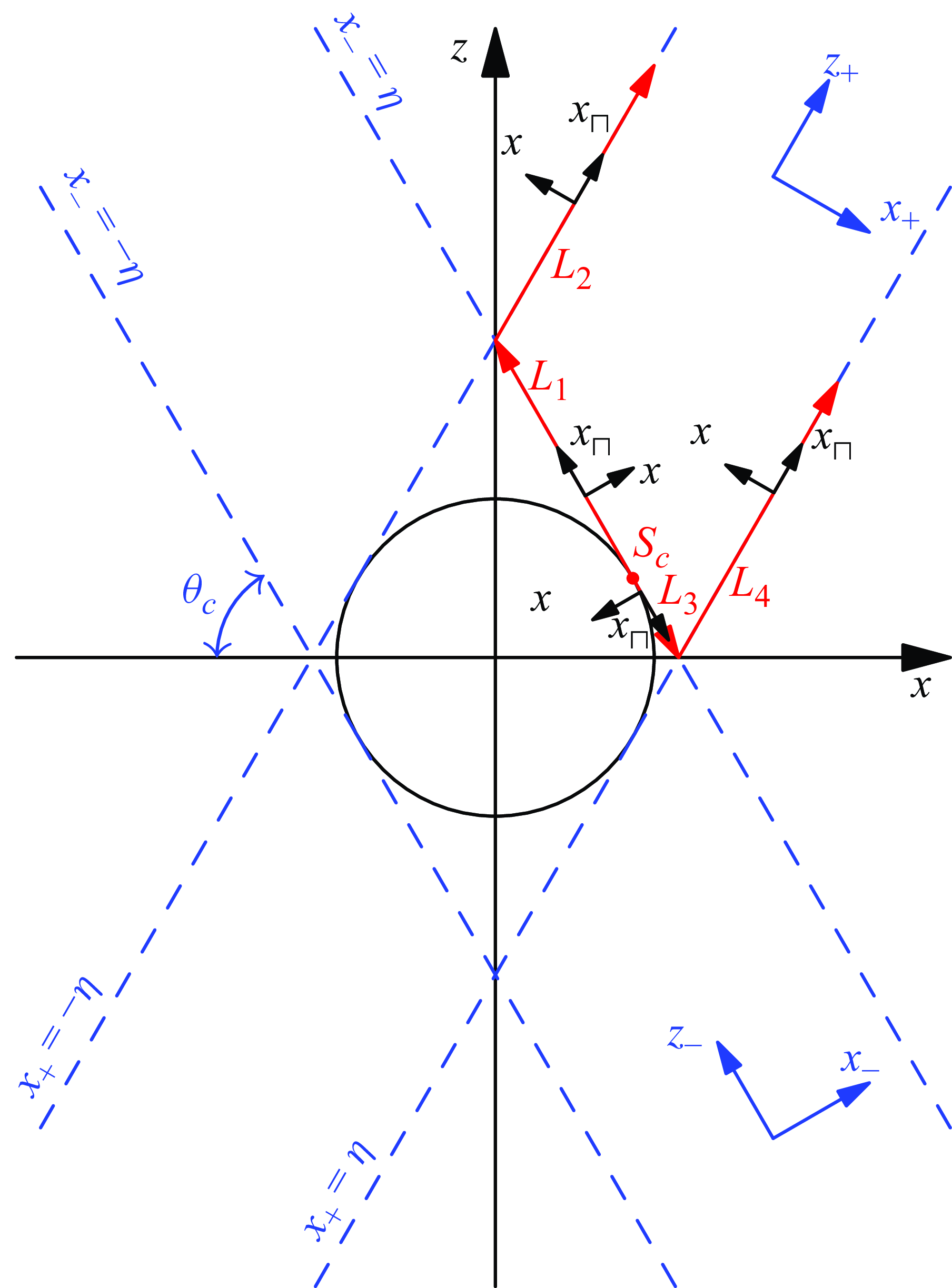
Tangent characteristic lines (blue dashed lines) of a cylinder in an unbounded domain. Here,
 $(x_{\pm} , z_\pm )$
are characteristic coordinates and
 $(x_\parallel , x_\perp )$
are local coordinates attached to critical rays
 $L_1 (x_-=\eta ; z_-\gt 0)$
,
 $L_2$
(
 $x_+=-\eta$
;
 $z_+\gt \eta$
),
 $L_3$
(
 $x_-=\eta$
;
 $z_-\lt 0$
) and
 $L_4$
(
 $x_+=\eta$
;
 $z_+\gt \eta$
) in the first quadrant.

In the inertial wave regime (
 $0\lt \omega \lt 2$
), the Poincaré equation (2.21) is a two-dimensional hyperbolic equation, the solution of which can be described in terms of its characteristics. As in Voisin (Reference Voisin2021), the global characteristic coordinates are defined as
 \begin{align} x_{\pm} =\sin \theta _cx\mp \cos \theta _cz, \quad z_\pm =\pm \cos \theta _c x+\sin \theta _c z, \end{align}
with
 \begin{align} \omega =2\cos \theta _c, \end{align}
where
 $\theta _c$
is the acute angle between the characteristics and the horizontal plane. The characteristic coordinates
 $x_{\pm }$
and
 $z_{\pm }$
are perpendicular and parallel to the characteristics, respectively; particularly,
 $|x_{\pm} |=\eta$
denote the positions of the characteristics tangent to the cylinder (see blue symbols in figure 2). The canonical form of the Poincaré equation (2.21) is simply
 $\partial ^2\psi /\partial x_+ \partial x_-=0$
; the corresponding solution is separable in terms of
 $x_{\pm}$
, namely,
 \begin{align} \psi (x_+,x_-)=\psi _+(x_+) + \psi _-(x_-). \end{align}
The corresponding velocity vector in the
 $Oxz$
plane is
 \begin{align} v_{z_+}\boldsymbol{e}_{z_+}+v_{z_-}\boldsymbol{e}_{z_-} ,\end{align}
with
 \begin{align} v_{z_\pm }(x_{\pm} )=\frac {{\textrm d}\psi _\pm }{{\textrm d}x_{\pm} }, \end{align}
where
 $\boldsymbol{e}_{z_\pm }$
are unit vectors in the
 $z_\pm$
directions. The velocity vector can be projected into the Cartesian coordinates, to yield the velocity components in the latter
 \begin{align} v_x=(v_{z_+}-v_{z_-})\cos \theta _c, v_z=(v_{z_+}+v_{z_-})\sin \theta _c, v_y = \frac {2}{\textrm{i}\omega }v_x=-\textrm{i}(v_{z_+}-v_{z_-}). \\[-9pt] \nonumber \end{align}
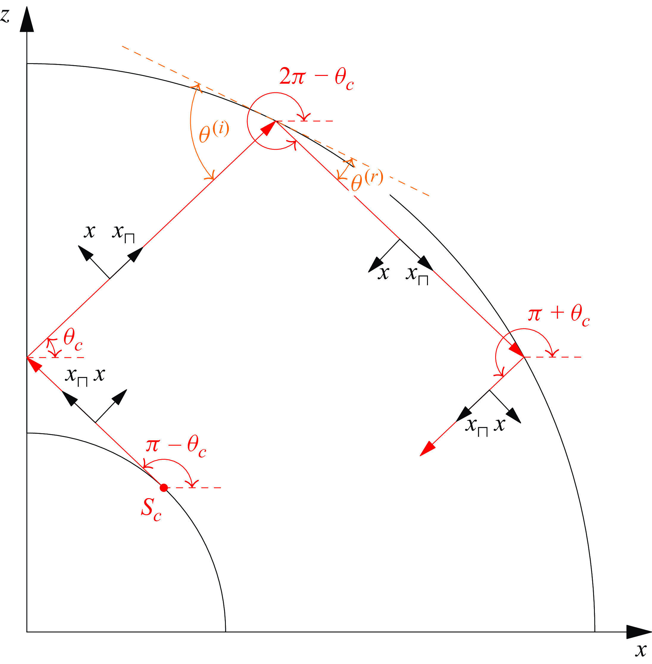
Critical rays with four different propagation directions (in red) and their local coordinates (in black). Schematic of the reflection on a boundary is shown in orange.

Usually, the inviscid solution may become singular on critical characteristics. In this case, it is preferable to describe the solution in terms of local coordinates (
 $x_\parallel , x_\perp$
) around the critical characteristics, where
 $x_\parallel$
measures the distance to the source along the critical characteristic and
 $x_\perp$
the displacement relative to it. The orientations of the local coordinates (
 $x_\parallel , x_\perp$
) depend on the direction of the wave propagation on the critical characteristics. For a fixed frequency
 $\omega$
that corresponds to a fixed
 $\theta _c$
, inertial waves propagate in four possible directions, which are
 $\theta _c$
,
 $\pi -\theta _c$
,
 $\pi +\theta _c$
and
 $2\pi -\theta _c$
with respect to the positive horizontal direction (see red symbols in figure 3). The direction of the local parallel coordinate
 $x_\parallel$
follows the propagation direction; the direction of the local perpendicular coordinate
 $x_\perp$
is chosen such that a nearby non-critical ray remains on the same side (with respect to positive or negative
 $x_\perp$
) of the critical ray after reflection (see black symbols in figure 3). In these local frames, the streamfunction is related to the local velocity components
 $(v_\parallel , v_\perp )$
through
 \begin{align} v_\parallel =\epsilon \frac {\partial \psi }{\partial x_\perp }, \quad v_\perp =-\epsilon \frac {\partial \psi }{\partial x_\parallel }, \end{align}
where
 $\epsilon =1$
for the rays with the inclined angles
 $\pi -\theta _c$
and
 $2\pi -\theta _c$
, and
 $\epsilon =-1$
for the rays with inclined angles
 $\theta _c$
and
 $\pi +\theta _c$
(see figure 3). In the inviscid case, the streamfunction and the parallel velocities depend on the local perpendicular coordinate
 $x_\perp$
only, namely,
 \begin{align} \psi (x_\perp ), \quad v_\parallel (x_\perp )=\epsilon \frac {\textrm{d}\psi (x_\perp )}{\textrm{d} x_\perp }. \end{align}
The velocity components
 $(v_x, v_z)$
in the Cartesian coordinates are obtained through projecting
 $v_\parallel \boldsymbol{e}_\parallel$
into the latter. Notably,
 $v_y$
is related to
 $v_\parallel$
through a phase shift, namely,
 \begin{align} v_{y}=\pm \textrm{i}v_\parallel . \end{align}
The sign of the phase is ‘+’ for the rays with the inclined angles
 $\pi -\theta _c$
and
 $\pi + \theta _c$
, and it is ‘−’ for the rays with the inclined angles
 $\theta _c$
and
 $2\pi -\theta _c$
(see figure 3).
2.4. Viscous similarity solution describing internal shear layers
Now we briefly describe the general asymptotic structure of internal shear layers, irrespective of the configurations. We only show the expressions in two dimensions that are relevant to the current work. Similar descriptions can be found in our previous works (Le Dizès & Le Bars Reference Le Dizès and Le Bars2017; He et al. Reference He, Favier, Rieutord and Le Dizès2022, Reference He, Favier, Rieutord and Le Dizès2023).
In the small viscosity limit (
 $E\rightarrow 0$
), the quantitative feature of the internal shear layers can be described by the famous similarity solution of Moore & Saffman (Reference Moore and Saffman1969), characterised by a width scaling as
 $E^{1/3}$
. This similarity solution is expressed in the local coordinates
 $(x_\parallel , x_\perp )$
described above. A similarity variable is introduced as
 \begin{align} \zeta =\frac {x_{\perp }}{E^{1/3}}\left (\frac {2\sin \theta _c}{x_\parallel }\right )^{1/3}. \end{align}
At leading order, the main velocity component is along the critical characteristics, namely
 $v_\parallel$
, which takes the form
 \begin{align} v_{\parallel }=C_0H_m(x_\parallel ,x_\perp )=C_0\left (\frac {x_\parallel }{2\sin \theta _c}\right )^{-m/3}h_m(\zeta ), \end{align}
with the special function introduced by Moore & Saffman (Reference Moore and Saffman1969)
 \begin{align} h_m(\zeta )=\frac {\textrm{e}^{-\textrm{i}m\pi /2}}{(m-1)!}\int ^{+\infty }_{0}\textrm{e}^{\textrm{i}p\zeta -p^3}p^{m-1}{\textrm d}p. \end{align}
The perpendicular velocity
 $v_\perp$
is
 $O(E^{1/3})$
smaller. Owing to the fluid rotation, the similarity solution also possesses a velocity component perpendicular to the plane (
 $\boldsymbol{e}_{\parallel }$
,
 $\boldsymbol{e}_\perp$
). It is related to
 $v_\parallel$
by a simple phase shift according to the relation (2.32).
There are two free parameters in the similarity solution (2.34): the amplitude
 $C_0$
and the index
 $m$
. The calculation of these parameters for each configuration constitutes the core of our work. It will mainly follow the line of our previous works (Le Dizès & Le Bars Reference Le Dizès and Le Bars2017; He et al. Reference He, Favier, Rieutord and Le Dizès2022, Reference He, Favier, Rieutord and Le Dizès2023) performed for a viscous forcing. One can first note that the similarity solution is indeed associated with an inviscid singularity, which is visible when considering the outer limit (
 $|\zeta | \rightarrow \infty$
) of the similarity solution
 \begin{align} v_{\parallel }\sim \left \{ \begin{array}{ll} C_0x_\perp ^{-m}E^{m/3}, & \zeta \rightarrow +\infty ; \\[6pt] C_0(-x_\perp )^{-m}\textrm{e}^{-\textrm{i}m\pi }E^{m/3}, & \zeta \rightarrow -\infty . \end{array}\right . \end{align}
Note the behaviour in
 $|x_\perp |^{-m}$
on both sides of the singularity. The index
 $m$
is then directly related to the strength of the underlying inviscid singularity. Note also the phase shift in
 $e^{-\textrm {i} m\pi }$
for
 $x_\perp \lt 0$
. This phase shift is associated with the direction of propagation of the singular field, which has to be in the direction of
 $+ {\boldsymbol e}_\parallel$
(Le Dizès Reference Le Dizès2024). The similarity solution (2.34) can be expressed in terms of a streamfunction
 $\psi$
. Integration of the similarity solution (2.34) leads to
 \begin{align} \psi =\epsilon \frac {C_0E^{1/3}}{m-1}H_{m-1}(x_\parallel ,x_\perp ). \end{align}
Note that, the streamfunction
 $\psi$
is
 $O(E^{1/3})$
smaller than
 $v_\parallel$
.
2.4.1. Reflections on boundaries and axes
In a bounded domain, the self-similar beam is expected to reflect on the boundaries. The reflection law, based on the preservation of the self-similar structure and the non-penetrability condition, has been discussed in Le Dizès (Reference Le Dizès2020) and He et al. (Reference He, Favier, Rieutord and Le Dizès2022, Reference He, Favier, Rieutord and Le Dizès2023). For an incident beam
 $v_{\parallel }^{(i)}=C_0^{(i)}H_m(x_{\parallel }^{(i)},x_{\perp }^{(i)})$
and its reflected counterpart
 $v_{\parallel }^{(r)}=C_0^{(r)}H_m(x_{\parallel }^{(r)},x_{\perp }^{(r)})$
, the conservation of the similarity variable and the non-penetrability condition lead to relations for the travelled distance and amplitude before and after the reflection
 \begin{align} \frac {x_{\parallel b}^{(r)}}{x_{\parallel b}^{(i)}}=\alpha ^3, \quad \frac {C_0^{(r)}}{C_0^{(i)}}=\alpha ^{m-1}, \end{align}
where the subscript
 $b$
indicates that the values are taken at the reflection point. The reflection factor
 $\alpha$
is given by
 \begin{align} \alpha =\frac {\sin \theta ^{(r)}}{\sin \theta ^{(i)}}, \end{align}
where
 $\theta ^{(r)}$
and
 $\theta ^{(i)}$
represent the angles of the reflected and incident beams relative to the tangent surface at the reflection point (see orange symbols in figure 3). The value, when compared with
 $1$
, indicates a contraction (
 ${\lt } 1$
) or expansion (
 ${\gt } 1$
) of the beam width. Notably, there is no contraction or expansion on the horizontal or vertical axis, and the reflection factor remains consistently equal to
 $1$
. The reflection law on a boundary (2.38) demonstrates that both the distance to the source and the amplitude are a priori modified by reflection.
The symmetries of the problem with respect to the
 $Ox$
and
 $Oz$
axes can be treated as reflection laws in the reduced domain that we consider (the upper-right quarter). Indeed, when a beam reaches the reduced domain boundary corresponding to one of the two axes, it effectively crosses the boundary and continues outside the reduced domain. However, the problem symmetry imposes that a symmetrical beam enters the reduced domain as the first beam leaves it. When this image beam is considered as a reflected beam, we can obtain reflection laws on the two axes as if they were real boundaries. These laws are obtained by writing the solution close to the axes as the sum of these two beams
 $v_{\parallel }^{(i)} (x_{\parallel }^{(i)},x_{\perp }^{(i)} )\boldsymbol{e}_{\parallel }^{(i)}+v_\parallel ^{(r)} (x_{\parallel }^{(r)},x_{\perp }^{(r)} )\boldsymbol{e}_{\parallel }^{(r)}$
. If we apply the conditions of symmetry (2.6)–(2.7) on this expression, we immediately obtain that
 $v_x$
should vanish on both axes. As
 $x_\perp ^{(r)} = x_\perp ^{(i)}$
on
 $Ox$
and on
 $Oz$
(see figure 3), we get that the reflection factor
 $\alpha$
is 1 for both axes. Similar to the reflection law on a boundary (2.38), we can then write the relations between the two beams as
 \begin{align} x_{\parallel b}^{(r)}=x_{\parallel b}^{(i)}, \quad C_0^{(r)}=\textrm{e}^{\textrm{i}\varphi }C_0^{(i)}, \end{align}
where the phase shift
 $\varphi$
is
 \begin{align} \varphi = \left \{ \begin{array}{ll} \pi , & \quad \textrm {on} \quad Ox, \\[2pt] 0, & \quad \textrm {on} \quad Oz. \end{array}\right . \end{align}
Therefore, the ‘reflection’ on the
 $Oz$
axis can be considered as a regular reflection on a vertical surface (i.e. without phase shift) while the “reflection” on the
 $Ox$
axis is a special reflection on an horizontal surface, as the reflected beam has gained a phase shift of
 $\pi$
.
3. Unbounded domain
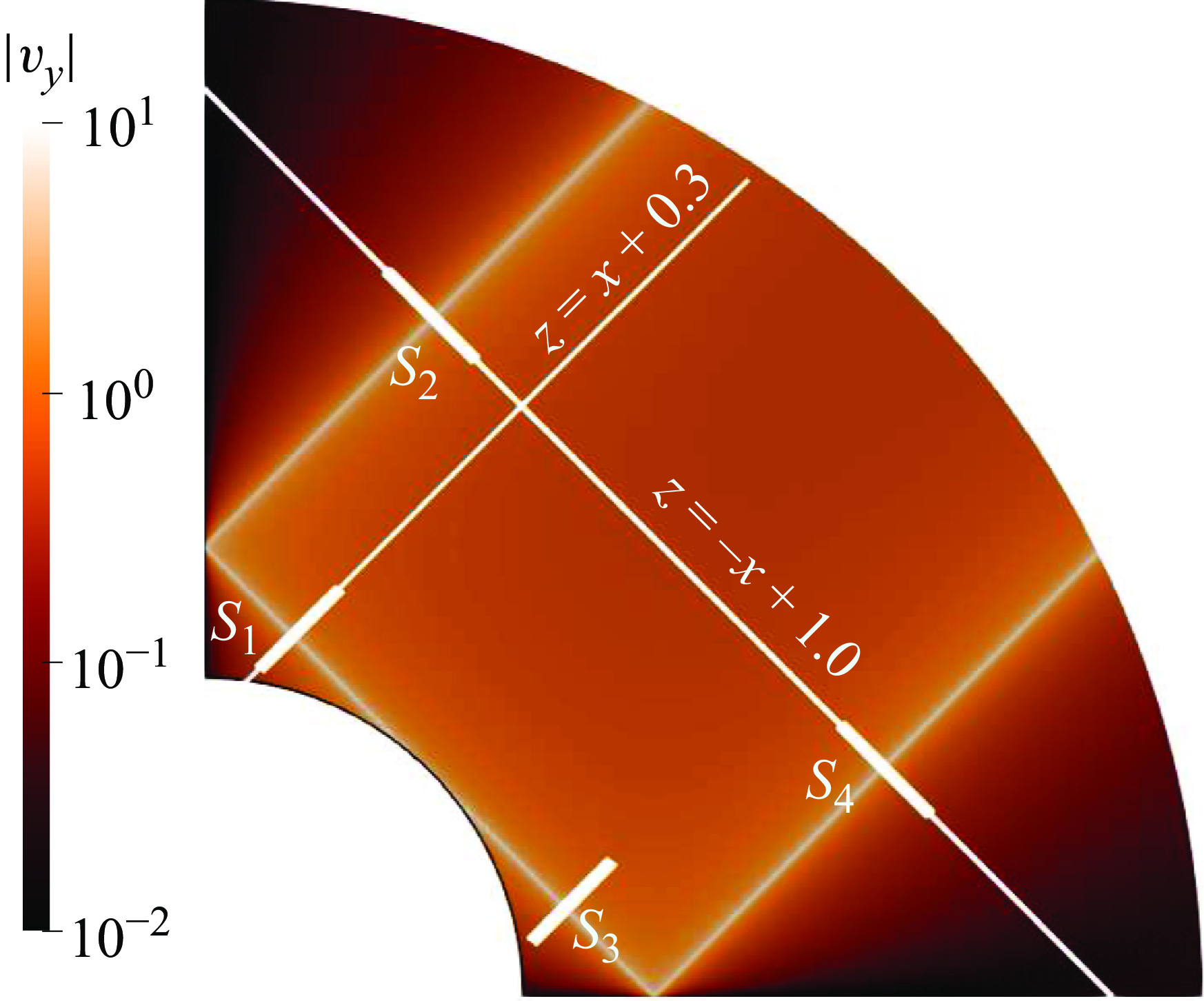
We first consider the unbounded domain, without outer cylinder. To illustrate the wave pattern, the numerical contours of
 $|v_y|$
are shown in figure 4 for the frequency
 $\omega =\sqrt {2}$
at the Ekman number
 $E=10^{-10}$
. We clearly observe strong shear layers originating from the critical points of the cylinder, where the local slope of the boundary coincides with one of the directions of propagation.
Contour of
 $|v_y|$
by numerical method for
 $\omega =\sqrt {2}$
, with
 $\eta =0.35$
and
 $E=10^{-10}$
in an unbounded domain. Numerical domain size is [0.35, 3.5], with sponge layer specified by
 $\Upsilon =\omega ^{-1}$
,
 $\varrho _s=2.45$
and
 $\Lambda =0.2$
(see (2.20)); the resolution is
 $N=3000$
and
 $L=6000$
; the result is shown in the truncated domain
 $[0.35, 1.1]$
.

In order to derive the similarity solutions for the internal shear layers around the tangent characteristics, there are two different technical paths. The first common step is to derive the global inviscid solution. Afterwards, the two paths diverge. One path is to obtain the local inviscid solutions around the tangent lines from the global inviscid solution and then obtain the local viscous solutions by matching the local inviscid solutions with the similarity solution. The other path is to obtain the global viscous solution by adding viscous attenuation to the global inviscid solution and then obtain the local viscous solutions around the tangent lines from the global viscous solution. One can clearly find that the second method is more advantageous, as no self-similar assumption of the internal shear layers shall be made. However, we will adopt the first method in the main text, as it is still effective and will also be adopted in the bounded domain. The details of the second method are shown in Appendix B. One should note that, the two methods yield the same expressions of the local viscous solutions around the tangent lines (see Appendix B).
3.1. Global inviscid solution
The global inviscid solution is obtained by solving the Poincaré equation (2.21) analytically, with the boundary condition at the surface of the cylinder (2.5)
 \begin{align} \psi =x \quad \textrm {at} \quad x^2+z^2=\eta ^2. \end{align}
Note that we have replaced the no-slip boundary condition with the free-slip counterpart. At the other end far from the cylinder, the streamfunction is allowed to freely radiate to infinity.
As discussed before, the Poincaré equation (2.21) in the inertial range
 $0\lt \omega \lt 2$
is actually a hyperbolic equation. A similar equation, along with the boundary condition (3.1), appears in studies of internal wave generation, where the analytical techniques for solving it are well developed (Appleby & Crighton Reference Appleby and Crighton1986, Reference Appleby and Crighton1987; Hurley Reference Hurley1997; Hurley & Keady Reference Hurley and Keady1997; Voisin Reference Voisin2003; Voisin, Ermanyuk & Flór Reference Voisin, Ermanyuk and Flór2011; Voisin Reference Voisin2021). The general technique involves solving an elliptic equation in the evanescent regime and analytically continuing the solution to the propagating regime. We can easily adapt this technique to our problem. We first solve the Poincaré equation (2.21) in the regime
 $\omega \gt 2$
where the equation is elliptic. Using a coordinate stretching similar to that of Voisin (Reference Voisin2021)
 \begin{align} x_\star =\frac {\sqrt {\omega ^2-4}}{2}x, \quad z_\star =\frac {\omega }{2}z, \end{align}
the elliptic equation (2.21) is recast into a standard Laplacian equation
 \begin{align} \frac {\partial ^2\psi }{\partial x_\star ^2}+\frac {\partial ^2\psi }{\partial z_\star ^2}=0, \end{align}
with the boundary condition specified at the surface of an ellipse
 \begin{align} \psi =\frac {2}{\sqrt {\omega ^2-4}}x_\star \quad \textrm {at} \quad \left (\frac {2x_\star }{\sqrt {\omega ^2-4}\eta }\right )^2+\left (\frac {2z_\star }{\omega \eta }\right )^2=1. \end{align}
The Laplacian equation for a region outside an ellipse can be solved analytically using elliptic coordinates
 \begin{align} x_\star =\eta \sinh \sigma \cos \tau , \quad z_\star =\eta \cosh \sigma \sin \tau , \end{align}
where
 $\sigma$
is a non-negative real number and
 $\tau \in [0,2\pi ]$
. Recasting the Laplacian equation into the
 $(\sigma ,\tau )$
coordinates and using separation of variables, we obtain the solution
 \begin{align} \psi (\sigma ,\tau )=\eta \frac {2}{\omega -\sqrt {\omega ^2-4}}\textrm{e}^{-\sigma }\cos \tau . \end{align}
The next step is to analytically continue the solution (3.6) from the evanescent regime
 $\omega \gt 2$
to the propagating regime
 $0\lt \omega \lt 2$
. The mathematical details of the analytical continuation are given in Appendix A. The solution (3.6) is analytically continued into the formula (2.26) with
 \begin{align} \psi _\pm =\tfrac {1}{2}\textrm{e}^{\textrm{i}(\theta _c-\pi /2)}\left [x_{\pm} -\sqrt {x_{\pm} ^2-\eta ^2}\right ], \end{align}
where the square root is determined by
 \begin{align} (x_{\pm} ^2-\eta ^2)^{1/2} = \left \{ \begin{array}{ll} |x_{\pm} ^2-\eta ^2|^{1/2}\textrm{sign}(x_{\pm} ), & |x_{\pm} |\gt \eta ; \\[5pt] \mp \textrm{i}|x_{\pm} ^2-\eta ^2|^{1/2}\textrm{sign}(z_\pm ), & |x_{\pm} |\lt \eta . \end{array} \right . \end{align}
The solution is separable in terms of the characteristic coordinates
 $x_{\pm}$
, which is a natural property of the two-dimensional hyperbolic equation.
Of particular interest are the velocities along the characteristics. They can be obtained by taking derivatives of
 $\psi _{\pm }$
with respect to
 $x_{\pm}$
(2.28), which leads to
 \begin{align} v_{z_\pm } = \tfrac {1}{2}\textrm{e}^{\textrm{i}(\theta _c-\pi /2)}\left (1-\frac {x_{\pm} }{\sqrt {x_{\pm} ^2-\eta ^2}}\right ). \end{align}
Thus, we have obtained the global inviscid velocities along the characteristics. Obviously, the global inviscid solution (3.9) is singular at the points where
 $|x_{\pm }|=\eta$
, that is on the characteristics tangent to the cylinder.
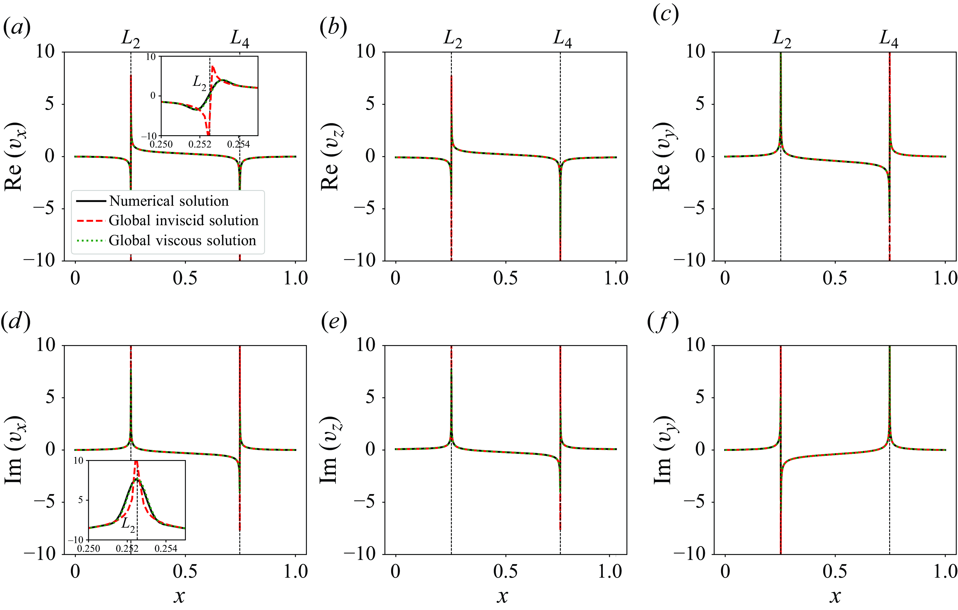
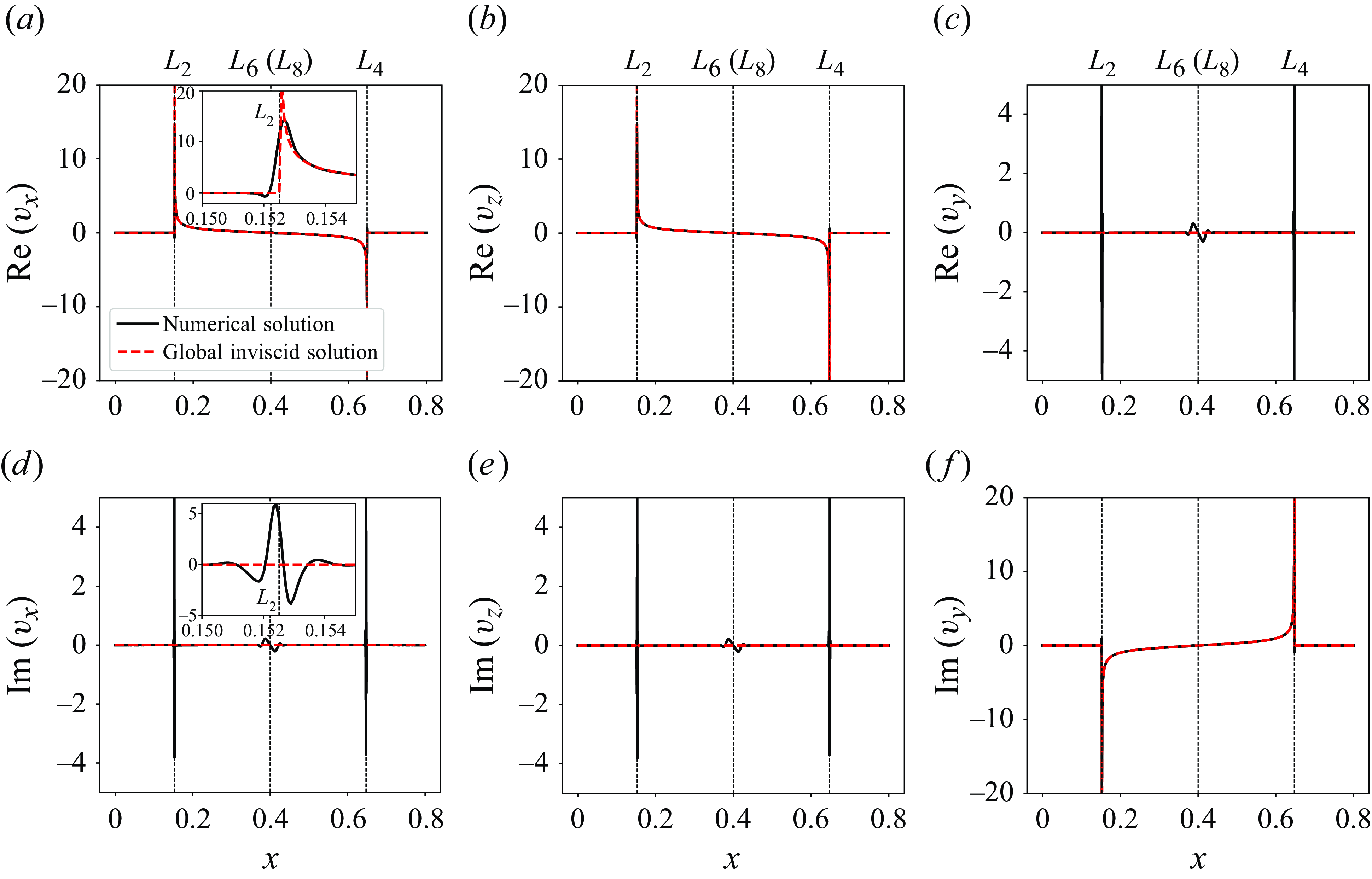
Comparison between numerical, global inviscid (3.9) and global viscous (B13) solutions for the unbounded case at
 $E=10^{-10}$
on the line
 $z=-x+1.0$
(see figure 4) for velocity components
 $v_x$
(
 $a,\!d$
),
 $v_z$
(
 $b,\!e$
) and
 $v_y$
(
 $c,\!f$
). Insets show local profiles around the critical line
 $L_2$
. The Jupyter notebook for producing the figure can be found at https://multimediafluids.uam.elogim.com/S0022112025102371/JFM-Notebooks/files/figure_5/figure_5.ipynb.

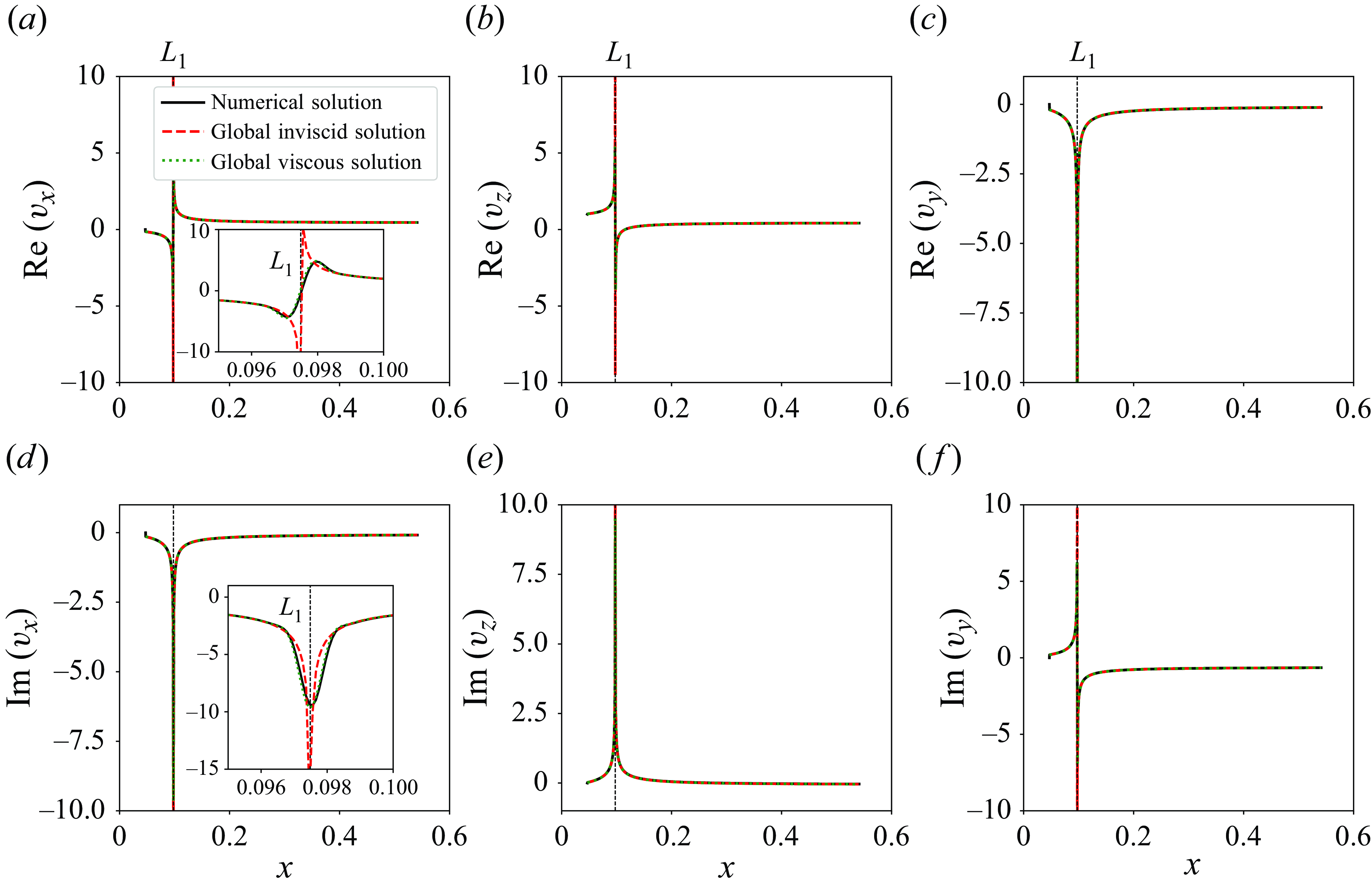
Similar comparison as figure 5 but for the line
 $z=x+0.3$
(see figure 4). Insets show local profiles around the critical line
 $L_1$
. The Jupyter notebook for producing the figure can be found at https://multimediafluids.uam.elogim.com/S0022112025102371/JFM-Notebooks/files/figure_6/figure_6.ipynb.

The velocity components
 $(v_x, v_z, v_y)$
in the Cartesian coordinates are related to
 $v_{z_\pm }$
by (2.29). In figures 5 and 6, we compare the global inviscid solution (3.9; red dashed lines) and the numerical counterpart (black solid lines) at
 $E=10^{-10}$
for the velocity profiles of
 $(v_x, v_z, v_y)$
along the cuts
 $z=-x+1.0$
and
 $z=x+0.3$
(see figure 4), respectively. The cut
 $z=-x+1.0$
goes through the critical lines
 $L_2$
and
 $L_4$
, while
 $z=x+0.3$
goes through
 $L_1$
(see figure 2). Far from the critical lines, the two solutions agree with each other very well at the small Ekman number. Close to the critical lines, the singularity of the inviscid solution is clearly visible, necessitating viscous smoothing.
3.2. Local inviscid solutions
Now we try to obtain the local inviscid solutions around the singular lines that will be utilised for asymptotic matching. Due to symmetry, we only consider the local inviscid solutions near the four critical rays
 $L_1-L_4$
in the first quadrant; see red arrows in figure 2. The definitions of the corresponding local coordinates for the four rays are shown in black in figure 2. The transformations between the local and global coordinates perpendicular to the characteristics are as follows:
 \begin{align} x_{\perp L_1}=x\_ - \eta ; \quad x_{\perp L_2}=-x_+-\eta ; \quad x_{\perp L_3}=-x_-+\eta ; \quad x_{\perp L_4}=-x_++\eta . \\[-15pt] \nonumber \end{align}
The positions of the tangent lines
 $|x_{\pm} |=\eta$
become simply
 $x_\perp =0$
in the local coordinates. The singular part of the global velocity
 $v_{z_\pm }$
(3.9) corresponds to the local parallel velocity
 $v_\parallel$
close to the critical characteristic. Thus, we obtain the local inviscid parallel velocity
 $v_\parallel$
along the lines
 $L_1-L_4$
as follows:
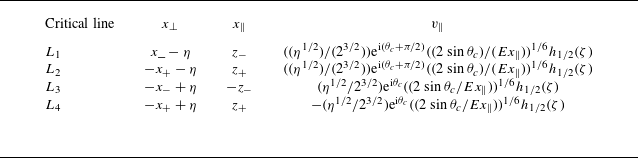
 \begin{align} v_\parallel = \frac {\sqrt {\eta }}{2\sqrt {2}}x_\perp ^{-1/2}\left \{ \begin{array}{ll} \textrm{e}^{\textrm{i}(\theta _c+\pi /2)}, & L_1; \\ \textrm{e}^{\textrm{i}(\theta _c+\pi /2)}, & L_2; \\ \textrm{e}^{\textrm{i}\theta _c}, & L_3; \\ \textrm{e}^{\textrm{i}(\theta _c-\pi )} & L_4. \end{array} \right . \end{align}
The phases are determined by the square roots in the global coordinates according to (3.8). Note that these solutions are only for the positive sides of the local perpendicular coordinates
 $x_\perp$
(see figure 2); the counterparts on the negative sides possess an additional phase
 $\textrm{e}^{-\textrm{i}\pi /2}$
.
3.3. Viscous similarity solutions
The matching of the local inviscid solutions (3.11) with the similarity solution (2.34) is straightforward. By doing so, we obtain the index
 \begin{align} m=1/2 ,\end{align}
and the amplitudes
 \begin{align} C_0 = \frac {\sqrt {\eta }}{2\sqrt {2}}E^{-1/6}\left \{ \begin{array}{ll} \textrm{e}^{\textrm{i}(\theta _c+\pi /2)}, & L_1; \\ \textrm{e}^{\textrm{i}(\theta _c+\pi /2)}, & L_2; \\ \textrm{e}^{\textrm{i}\theta _c}, & L_3; \\ \textrm{e}^{\textrm{i}(\theta _c-\pi )} & L_4. \end{array} \right . \end{align}
Obviously, the amplitudes scale with the Ekman number as
 $E^{-1/6}$
. Note that, there is no phase shift from
 $L_1$
to
 $L_2$
on the vertical axis
 $Oz$
, and there is a phase shift of
 $\pi$
from
 $L_3$
to
 $L_4$
on the horizontal axis
 $Ox$
. These are consistent with the phase shifts (2.40) that were obtained from symmetry conditions directly.
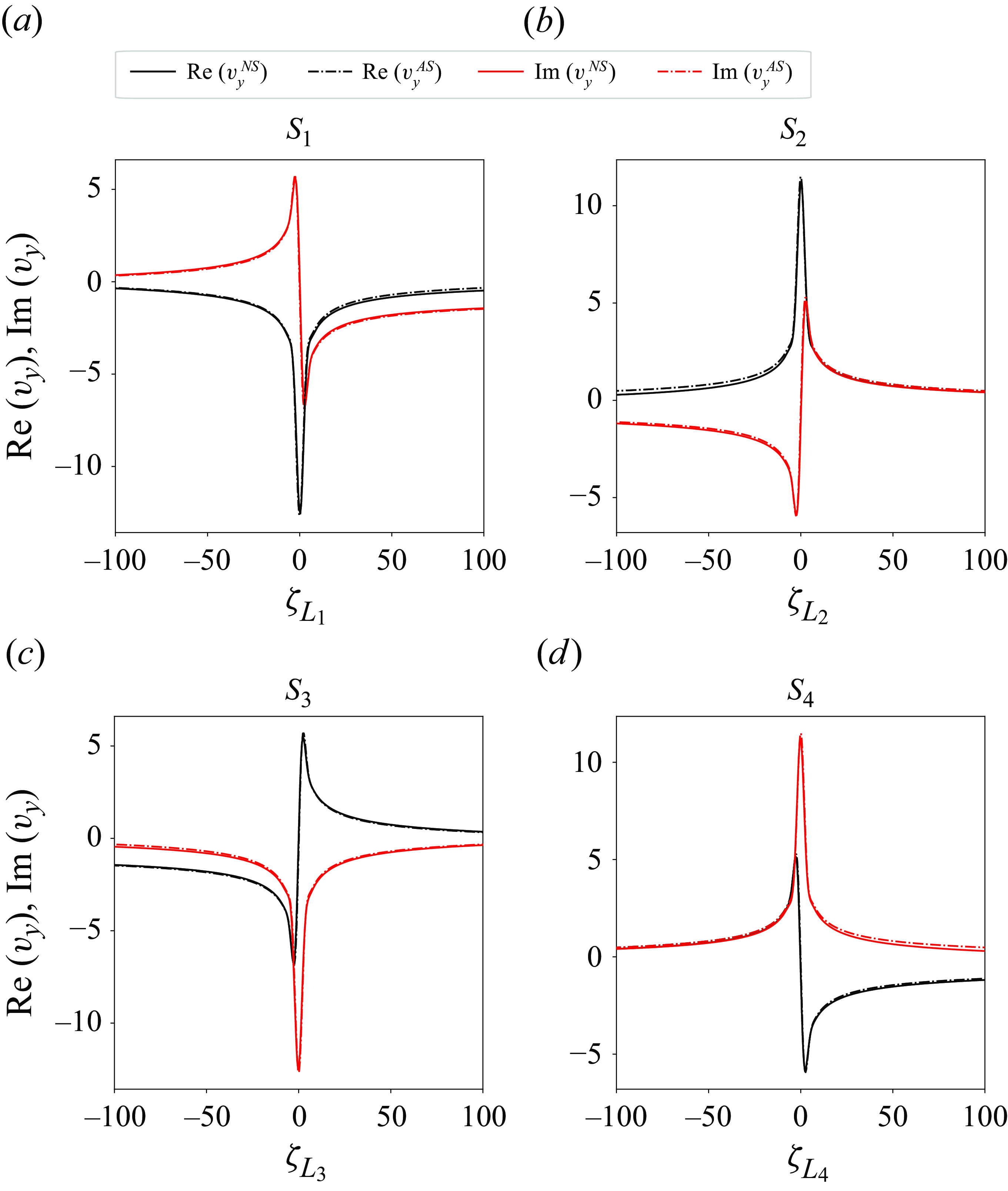
Comparison of velocity profiles between the numerical (superscript “NS”) and asymptotic (superscript “AS”) solutions for
 $v_y$
at
 $E=10^{-10}$
on the four short white cuts
 $S_1-S_4$
shown in figure 4. The Jupyter notebook for producing the figure can be found at https://multimediafluids.uam.elogim.com/S0022112025102371/JFM-Notebooks/files/figure_7/figure_7.ipynb.

After obtaining the index and the amplitudes, we need to determine the local coordinates before calculating the asymptotic solutions. The coordinate
 $x_{\perp }$
can be measured according to the definitions shown in figure 2. Determining the parallel coordinates
 $x_\parallel$
requires information about the source position (
 $x_\parallel =0$
). As in Le Dizès & Le Bars (Reference Le Dizès and Le Bars2017), the critical point (
 $S_c$
in figure 2) is considered as the source, from which two rays propagate northward and southward, travelling along the ray paths
 $L_1\rightarrow L_2$
and
 $L_3\rightarrow L_4$
, respectively. Thus,
 $x_\parallel$
for each line is calculated by measuring the distance to the critical point along the ray path.
The excellent performance of the asymptotic solutions against the numerical solutions is shown in figure 7 for the velocity profiles
 $v_y$
at the Ekman number
 $E=10^{-10}$
around the four critical lines
 $L_1-L_4$
.
4. Bounded domain
In a bounded domain, the geometry of the characteristics becomes important. In a cylindrical annulus of fixed aspect ratio, the characteristic patterns only depend on the forcing frequency. As shown by Rieutord, Georgeot & Valdettaro (Reference Rieutord, Georgeot and Valdettaro2001), characteristics either form periodic orbits or attractors. Both ray patterns were considered in He et al. (Reference He, Favier, Rieutord and Le Dizès2022, Reference He, Favier, Rieutord and Le Dizès2023) in the case of a viscous forcing. In these works, the asymptotic solution was obtained by propagating the similarity solutions from the critical point with the amplitudes obtained from the unbounded domain analysis. This approach has been theoretically justified by Le Dizès (Reference Le Dizès2024). In that case, the author showed that the characteristics of the similarity solution only depend on the local property of the viscous forcing close to critical point. Le Dizès (Reference Le Dizès2024) also explained that this result is not valid for an inviscid forcing. The amplitude of the similarity solution in a closed geometry is expected to depend on the global ray pattern.
As in the unbounded domain considered in § 3, we shall first derive an inviscid solution. Unfortunately, a global inviscid solution in a cylindrical annulus cannot be obtained by separation of variables, since the Poincaré equation (2.21) is not separable on both boundaries (Rieutord et al. Reference Rieutord, Georgeot and Valdettaro2001). However, in two dimensions, one can use the method of characteristics. The expressions for the streamfunction and velocities (2.26)–(2.28), which are dependent of the global characteristic coordinates
 $x_{\pm}$
, are valid in the whole domain. They can be used to obtain equations involving
 $v_{z\pm }$
or
 $\psi _{\pm }$
by propagating the boundary conditions along the lines
 $x_{\pm} =\text{const}$
. This is the method of characteristics (Maas & Lam Reference Maas and Lam1995; Ogilvie Reference Ogilvie2005) that we shall use for both periodic orbits and attractors.
4.1. Periodic orbits
Similar to He et al. (Reference He, Favier, Rieutord and Le Dizès2022), we consider the simple periodic orbit at the frequency
 $\omega =\sqrt {2}$
and aspect ratio
 $\eta =0.35$
. The corresponding inclined angle is
 $\theta _c=\pi /4$
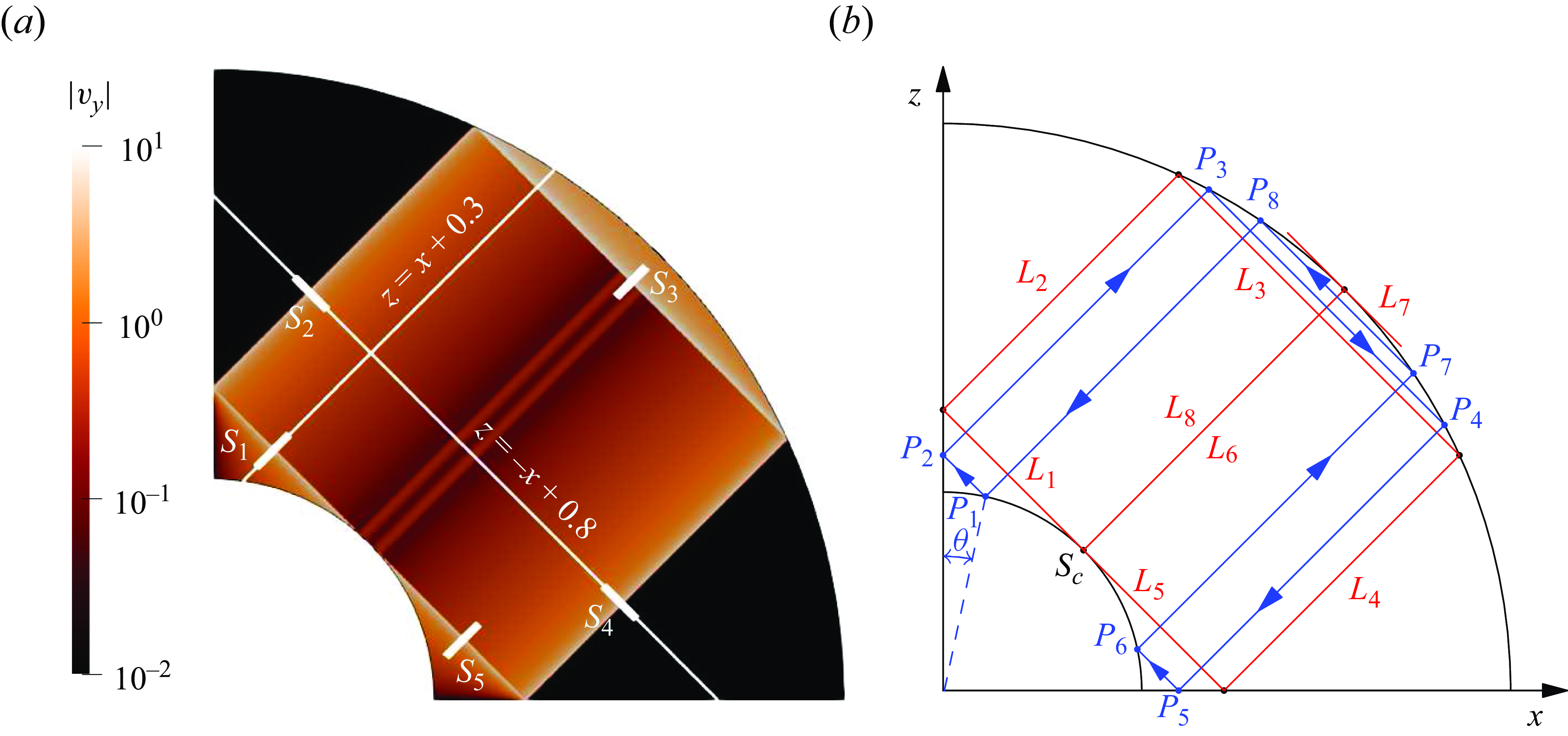
. Figure 8
 $(a)$
shows the numerical result for the amplitude of
 $v_y$
at
 $E=10^{-11}$
, where internal shear layers are observed around the critical characteristics
 $L_1-L_8$
issued from the critical point
 $S_c$
(see figure 8
 $b$
). One also clearly notices that the solution is much larger within the area enclosed by the critical lines and boundaries than in the rest of the domain.
Periodic orbit in a bounded domain for
 $\eta =0.35$
and
 $\omega =\sqrt {2}$
:
 $(a)$
numerical result of
 $|v_y|$
at
 $E=10^{-11}$
with the resolution
 $(N,L)=(2500,8000)$
;
 $(b)$
critical characteristics
 $L_1-L_8$
(red colour) and a neighbouring ray path
 $P_1P_2P_3P_4P_5P_6P_7P_8$
(blue colour) with the co-latitude
 $\theta$
. Note that
 $L_6$
coincides with
 $L_8$
.

4.1.1. Global inviscid solutions
To derive the inviscid solution for this particular ray pattern, we consider an arbitrary circuit issued from a point on the inner boundary different from
 $S_c$
, as shown by the blue lines
 $P_1P_2P_3P_4P_5P_6P_7P_8P_1$
in figure 8
 $(b)$
. The circuit is entirely determined by the co-latitude angle
 $\theta$
of the point
 $P_1$
on the inner boundary. We denote by
 $v_{\parallel j}$
the velocity along the segment
 $P_jP_{j+1}$
(
 $j=1,2,3,\ldots ,8$
,
 $P_9=P_1$
) in the direction
 $P_j\rightarrow P_{j+1}$
, as indicated in figure 8
 $(b)$
. If
 $x_{\pm j}$
denotes the constant value of
 $x_{\pm}$
on each segment
 $P_jP_{j+1}$
using the convention defined in figure 2, the velocity
 $v_{\parallel j}$
corresponds to
 $v_{z_-}(x_{- })$
for
 $j= 1,5,7$
,
 $-v_{z_-}(x_{- })$
for
 $j=3$
,
 $v_{z_+}(x_{+ })$
for
 $j=2,6$
and
 $-v_{z_+}(x_{+ })$
for
 $j=4,8$
.
According to the non-penetrability conditions on the boundaries and symmetry conditions on the axes, the velocities
 $v_{\parallel j}$
of the segments are related to each other by
 \begin{align}& v_{\parallel 1}\sin {(\pi /4-\theta )}-v_{\parallel 8}\sin {(\pi /4+\theta )}=\cos {\theta }, \\[-12pt] \nonumber \end{align}
 \begin{align}&\qquad\qquad\qquad\,\,\, v_{\parallel 2}=v_{\parallel 1}, \\[-12pt] \nonumber \end{align}
 \begin{align}&\qquad\qquad\qquad v_{\parallel 3}=v_{\parallel 2}/k_3, \\[-12pt] \nonumber \end{align}
 \begin{align}&\qquad\qquad\qquad v_{\parallel 4}=v_{\parallel 3}/k_4, \\[-12pt] \nonumber \end{align}
 \begin{align}&\qquad\qquad\qquad\, v_{\parallel 5}=-v_{\parallel 4}, \\[-12pt] \nonumber \end{align}
 \begin{align}& v_{\parallel 6}\sin {(\pi /4+\theta )}-v_{\parallel 5}\sin {(\pi /4-\theta )}=\sin {\theta }, \\[-12pt] \nonumber \end{align}
 \begin{align}&\qquad\qquad\qquad v_{\parallel 7}=v_{\parallel 6}/k_7, \\[-12pt] \nonumber \end{align}
 \begin{align}&\qquad\qquad\qquad v_{\parallel 8}=v_{\parallel 7}/k_8, \\[6pt] \nonumber \end{align}
where the reflection coefficients on the outer boundary are
 \begin{align} k_3=\frac {1}{k_4}=\frac {\eta \sin {(\pi /4+\theta )}}{\sqrt {1-\eta ^2\sin ^2(\pi /4+\theta )}}, \quad k_7=\frac {1}{k_8}=\frac {\eta \sin {(\pi /4-\theta )}}{\sqrt {1-\eta ^2\sin ^2(\pi /4-\theta )}}. \end{align}
By symmetry, one has
 $v_{\parallel 2}=v_{\parallel 4}$
, and
 $v_{\parallel 6} = v_{\parallel 8}$
. The relations (4.1) can thus be reduced to two functional equations for
 $v_{\parallel 1}$
and
 $v_{\parallel 8}$
, namely,
 \begin{align}& v_{\parallel 1}\sin {(\pi /4-\theta )}-v_{\parallel 8}\sin {(\pi /4+\theta )}=\cos {\theta }, \end{align}
 \begin{align}&\, v_{\parallel 1}\sin {(\pi /4-\theta )}+v_{\parallel 8}\sin {(\pi /4+\theta )}=\sin {\theta }. \end{align}
By solving the above equations for
 $v_{\parallel 1}$
and
 $v_{\parallel 8}$
and using the relations for the other components, we can obtain unique expressions for
 $v_{\parallel j}$
as functions of the co-latitude
 $\theta$
, namely,
 \begin{align}& v_{\parallel 1}=v_{\parallel 2}=v_{\parallel 4}=-v_{\parallel 5}=\frac {1}{\sqrt {2}}\frac {\sin {(\pi /4+\theta )}}{\sin {(\pi /4-\theta )}}, \\[-12pt] \nonumber \end{align}
 \begin{align}&\qquad v_{\parallel 3}=\frac {1}{\sqrt {2}}\frac {\sqrt {1-\eta ^2\sin ^2(\pi /4+\theta )}}{\eta \sin (\pi /4-\theta )}, \\[-12pt] \nonumber \end{align}
 \begin{align}&\qquad\, v_{\parallel 6}=v_{\parallel 8}=-\frac {1}{\sqrt {2}}\frac {\sin {(\pi /4-\theta )}}{\sin {(\pi /4+\theta )}}, \\[-12pt] \nonumber \end{align}
 \begin{align}&\quad\,\,\, v_{\parallel 7}=-\frac {1}{\sqrt {2}}\frac {\sqrt {1-\eta ^2\sin ^2(\pi /4-\theta )}}{\eta \sin (\pi /4+\theta )}, \\[6pt] \nonumber \end{align}
with
 $\theta \in [0, \pi /4]$
.
The above global inviscid solutions apply only to the area swept by the circuit
 $P_1\cdots P_8P_1$
with
 $\theta \in [0, \pi /4]$
, which is on one side of the critical lines (see figure 8
 $b$
). On the other side, the ray path does not touch the inner boundary and is not forced. The solution is therefore undetermined in this region. We choose to put it to zero. This choice is consistent with the numerical results displayed in figure 8(
 $a$
): the two regions which are not touched by rays emitted from the inner core are indeed black, which corresponds to a small amplitude.
The above expressions (4.4) can be rewritten in terms of the characteristic variables
 $(x_+, x_-)$
defined in (2.24). By doing so, we obtain the functions
 $v_{z\pm }(x_{\pm} )$
that appear in (2.27), as we did for the unbounded domain (see expression (3.9)). The result is
 \begin{align} v_{z_+}= \frac {1}{\sqrt {2}}\left \{ \begin{array}{ll} 0, & x_+\lt -\eta ; \\[3pt] \frac {-x_+}{\sqrt {\eta ^2-x_+^2}}, & -\eta \lt x_+\lt \eta ; \\[12pt] 0, & x_+\gt \eta , \end{array} \right . \end{align}
and
 \begin{align} v_{z_-}= \frac {1}{\sqrt {2}}\left \{ \begin{array}{ll} \textrm{sign}(x_+)\frac {-x_-}{\sqrt {\eta ^2-x_-^2}}, & \frac {\eta }{\sqrt {2}}\lt x_-\lt \eta ; \\[3pt] 0, & \eta \lt x_- \lt \sqrt {1-\eta ^2}; \\[5pt] \frac {-x_-}{\sqrt {x_-^2-(1-\eta ^2)}}, & \sqrt {1-\eta ^2} \lt x_- \lt 1. \end{array} \right . \end{align}
Note that the same term
 $\sqrt {x_{\pm} ^2-\eta ^2}$
appears in formula (3.9) and (4.5)–(4.6) thanks to the use of
 $\eta$
for the radius of the oscillating cylinder in both the unbounded and bounded cases. The expression (4.5) for
 $v_{z_+}$
is singular at
 $x_+=\pm \eta$
, which correspond to the critical lines
 $L_2$
and
 $L_4$
; the expression (4.6) for
 $v_{z_-}$
is singular at
 $x_-=\eta$
and
 $x_-=\sqrt {1-\eta ^2}$
, which correspond to the critical lines
 $L_1$
,
 $L_5$
and
 $L_3$
. For instance, close to
 $L_1$
, one has, as
 $x_- \rightarrow \eta$
 \begin{align} v_{z_-} \sim \left \{ \begin{array}{ll} \displaystyle \frac {\sqrt {\eta }}{2\sqrt {\eta -x_-}} , & x_-\lt \eta ; \\ 0, & \eta \lt x_- . \end{array} \right . \end{align}
Note that on the line
 $L_6$
(or
 $L_8$
) corresponding to
 $x_+=0$
, no singularity is present.
Comparison between inviscid and numerical solutions for the periodic orbit case on the line
 $z=-x+0.8$
(see figure 8
 $a$
) for velocity components
 $v_x$
(
 $a,\!d$
),
 $v_z$
(
 $b,\!e$
) and
 $v_y$
(
 $c,\!f$
) at
 $E=10^{-11}$
. Insets show local profiles around the critical line
 $L_2$
. The Jupyter notebook for producing the figure can be found at https://multimediafluids.uam.elogim.com/S0022112025102371/JFM-Notebooks/files/
figure_9/figure_9.ipynb.

Similar comparison as figure 9 but on the cut
 $z=x+0.3$
(see figure 8
 $a$
). The Jupyter notebook for producing the figure can be found at https://multimediafluids.uam.elogim.com/S0022112025102371/JFM-Notebooks/files/figure_10/figure_10.ipynb.

With the expressions (4.5)–(4.6) for
 $v_{z_\pm }$
, the velocity components
 $(v_x, v_z, v_y)$
are obtained through the transforms (2.29). In figures 9 and 10, we compare the global inviscid solution (4.5)–(4.6) with the numerical solution obtained at
 $E=10^{-11}$
for the velocity profiles of
 $(v_x, v_z, v_y)$
along the cuts
 $z=-x+0.8$
and
 $z=x+0.3$
(see figure 8
 $a$
), respectively. The cut
 $z=-x+0.8$
goes through the critical lines
 $L_2$
,
 $L_4$
and
 $L_6$
(or
 $L_8$
), while
 $z=x+0.3$
goes through
 $L_1$
and
 $L_3$
(see figure 8
 $b$
). Far from the critical lines, the two solutions agree with each other very well. On the other hand, near the critical lines, the inviscid solution fails to capture the local shear-layer structures (see insets in figures 9
 $d$
and 10
 $d$
), similar to the unbounded case. Close to the critical lines, viscosity has to be introduced to smooth out the singularity. It is the subject of the next subsection.
4.1.2. Viscous solution close to the critical line
We are going to construct a viscous solution close to the critical line following the approach that has been described in He et al. (Reference He, Favier, Rieutord and Le Dizès2022). The idea is to assume that the critical point
 $S_c$
is the singularity source, from which two singular beams are generated on either side of
 $S_c$
and along
 $L_1$
and
 $L_5$
. These beams are assumed to have the similarity form (2.34) described in § 2.4. Based on the nature of the singularity of the inviscid solution in
 $|x_\perp |^{-1/2}$
, one can expect that the similarity solution describing these beams will have an index
 $m=1/2$
. Nevertheless, we shall keep this parameter undetermined as well as the complex amplitudes of the similarity solution generated on each side.
Starting from the critical point, the northward beam will travel along the circuit
 $L_1\rightarrow L_2\rightarrow \cdots \rightarrow L_5$
, while the southward beam follows the opposite direction. Here,
 $L_1$
and
 $L_5$
are the initial segments for the northward and southward beams, respectively. Since the ray path is periodic, wave beams will return to the critical point after one cycle. They will then continue to propagate for another cycle, and so on, until they are fully dissipated by viscosity. For the
 $n$
th cycle on the segment
 $L_j$
, the asymptotic solution of the northward or southward beam is denoted as
 \begin{align} v_{\parallel j,n}=C_{j,n}H_m(x_{\parallel j,n}, \zeta _{j,n}), \end{align}
where the first subscript
 $j$
denotes the segment
 $L_j$
and the second subscript
 $n$
denotes the
 $n$
th cycle (
 $n=0$
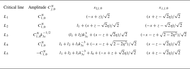
being for the very first cycle). The expressions of the amplitudes and local coordinates for
 $n=0$
are determined by reflection laws on the axes and boundaries. They have been derived for each segment in He et al. (Reference He, Favier, Rieutord and Le Dizès2022). For completeness, we have reproduced these results in Appendix C. For the subsequent cycles, the perpendicular coordinate remains unchanged, while the amplitude and parallel coordinate are modified, as explained in He et al. (Reference He, Favier, Rieutord and Le Dizès2022). They can be expressed in terms of the values obtained for the first cycle
 $n=0$
as
 \begin{align}&\quad\,\, x_{\parallel {j,n}}=x_{\parallel {j,0}}+n\mathcal{L}_j, \end{align}
 \begin{align}& \zeta _{j,n} = \zeta _{j,0}(x_{\parallel j,n}/x_{\parallel j,0})^{1/3}, \end{align}
 \begin{align}&\qquad C_{j,n} = C_{j,0} \textrm{e}^{\textrm{i} n\pi }. \\[6pt] \nonumber \end{align}
After one cycle, the parallel coordinate increases by the distance travelled along the closed circuit
 $\mathcal{L}_j$
(see (C2)); the amplitude is modified by a phase shift
 $\pi$
which is acquired at the reflection on the horizontal axis
 $Ox$
.
The final asymptotic solution is the sum of all
 $v_{\parallel j,n}$
from
 $n=0$
to
 $+\infty$
. As demonstrated by He et al. (Reference He, Favier, Rieutord and Le Dizès2022), this infinite series converges to a finite value if there exists a non-zero phase shift after the completion of each cycle. This requirement is satisfied as the phase shift along one cycle is
 $\pi$
. The resulting expression for the segment
 $L_j$
is
 \begin{align} v_{\parallel j} = \lim _{N\rightarrow +\infty }\sum _{n=0}^{N}v_{\parallel j,n}= C_{j,0} G_m(x_{\parallel j,0}, x_{\perp j,0}, \mathcal{L}_j), \end{align}
with
 \begin{align}& G_m(x_{\parallel },x_{\perp },\mathcal{L})=\left (\frac {x_{\parallel }}{2\sin \theta _c}\right )^{-m/3}g_m(\zeta , \mathcal{L}/x_{\parallel }), \end{align}
 \begin{align}& g_m(\zeta , \mathcal{L}/x_{\parallel })=\frac {\textrm{e}^{-\textrm{i} m\pi /2}}{(m-1)!}\int _0^\infty \frac {\textrm{e}^{\textrm{i} p\zeta -p^3}p^{m-1}}{1+\textrm{e}^{-p^3\mathcal{L}/x_{\parallel }}}{\textrm d}p. \end{align}
Note that the solution is expressed in terms of the variables in the very first cycle (
 $n=0$
) only. The above discussion holds both for the northward and southward beams. Finally, the asymptotic solution is the sum of two contributions, namely,
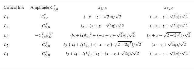
 \begin{align} v_{\parallel j}=C_{j,0}^{N} G_m(x_{\parallel j,0}^{N},x_{\perp j,0}^{N},\mathcal{L}_j)+C_{j,0}^{S} G_m(x_{\parallel j,0}^{S},x_{\perp j,0}^{S},\mathcal{L}_j), \end{align}
with ‘N’ and ‘S’ denoting ‘northward’ and ‘southward’, respectively. The amplitudes and local coordinates for the very first cycle (
 $n=0$
) are given in Appendix C in tables 3 and 4 for the northward and southward beams, respectively. The orientation of
 $v_{\parallel j}$
is given in figure 3. It corresponds to the orientation of the northward beam. From
 $v_{\parallel j}$
, one can deduce the corresponding transverse velocity component
 $v_y$
using (2.32).
We are now able to do the matching of this expression with the behaviour of the global inviscid solution close to the critical line. The behaviour of the asymptotic solution (4.12) as one goes away from the critical line is easily obtained using
 \begin{align} G_m(x_\parallel , x_\perp ) \sim \left \{ \begin{array}{ll} \frac {1}{2} x_\perp ^{-m}E^{m/3}, & \zeta \rightarrow +\infty \\[6pt] \frac {1}{2} (-x_\perp )^{-m}\textrm{e}^{-\textrm{i}m\pi }E^{m/3}, & \zeta \rightarrow -\infty . \end{array}\right . \end{align}
It gives for example on
 $L_1$
 \begin{align} v_{\parallel 1}=v_{z_-} \sim \left \{ \begin{array}{ll} \frac {1}{2} x_{\perp 1}^{-m}E^{m/3} (C_{1,0}^{N} - \textrm{e}^{-\textrm{i}m\pi } C_{5,0}^{S} ) , & x_{\perp 1} \gt 0 \\[5pt] \frac {1}{2} (-x_{\perp 1})^{-m}E^{m/3} (C_{1,0}^{N}\textrm{e}^{-\textrm{i}m\pi } - C_{5,0}^{S} ) , & x_{\perp 1} \lt 0 , \end{array}\right . \end{align}
where
 $x_{\perp 1} = x_- -\eta =(x+z-\sqrt {2}\eta )/\sqrt {2}$
is the local coordinate of the northward beam (see table 3). Note that we have replaced
 $C_{1,0}^{S}$
with
 $-C_{5,0}^{S}$
using the relation in the second column of the last row of the table 4.
The matching of these behaviours with the inviscid solution around
 $L_1$
(4.7) immediately gives
 $m=1/2$
, as expected, and
 \begin{align} C_{1,0}^{N} = \frac {\sqrt {\eta }}{2}\textrm{e}^{\textrm{i}\pi /2}E^{-1/6}, \quad C_{5,0}^{S}=\frac {\sqrt {\eta }}{2}E^{-1/6}. \end{align}
One can then check that with these values, we recover the behaviour of the global inviscid solution close to the other lines
 $L_j$
,
 $j=2,\ldots ,5$
.
It is interesting to compare these expressions with those obtained in an unbounded domain (compare (3.13a
) with (4.15a
) for the northward beam and (3.13c
) with (4.15b
) for the southward beam). They both scale as
 $E^{-1/6}$
and exhibit a
 $\pi /2$
phase shift between northward and southward beams. Yet, the norm and the phase of the beam amplitudes are different in unbounded and bounded cases.
It is also worth mentioning that (4.15) could have been deduced using another argument. Le Dizès (Reference Le Dizès2024) demonstrated that the singular beams emitted along
 $L_1$
and
 $L_5$
from
 $S_c$
depend on the waves emitted along the characteristic direction
 $L_6$
(
 $L_8$
), see figure 8(b). In the unbounded case, the waves emitted in that direction have a specific expression that was deduced from the global inviscid solution. For the bounded case with periodic orbits, we claim that nothing can be emitted along
 $L_6$
. The reason is the boundary condition on
 $L_6$
on the outer core which imposes the vanishing of the normal velocity, that is the vanishing of the velocity on
 $L_6$
. The amplitude of the singular beams emitted along
 $L_1$
and
 $L_5$
is then completely determined by the local behaviour around
 $S_c$
in that case. More precisely, if one uses equations (49) and (57a,b) of Le Dizès (Reference Le Dizès2024) with
 $F'(0)=0$
in (49), expressions (4.15a
,
b
) are recovered.
Comparison of velocity profiles (
 $v_y$
) between the numerical and asymptotic solutions for the periodic orbit case at
 $E=10^{-11}$
on the five cuts
 $S_1-S_5$
shown in figure 8. The Jupyter notebook for producing the figure can be found at https://multimediafluids.uam.elogim.com/S0022112025102371/JFM-Notebooks/files/figure_11/figure_11.ipynb.

In figure 11, the asymptotic solution (4.12) obtained with
 $C_{j,0}^{N}$
and
 $C_{j,0}^{S}$
given by (4.15a
,
b
) is compared with the numerical solution obtained for
 $E= 10^{-11}$
. This comparison is done for the velocity profiles
 $v_y$
on the five cuts
 $S_1 - S_5$
, shown in figure 8. We can see that the agreement is excellent on all the cuts. This confirms that the asymptotic solution derived above describes correctly the solution close to the critical line in the limit of small Ekman numbers.
Note that we have not derived the viscous solutions for the weaker internal shear layers around
 $L_6$
(
 $L_8$
) (see figure 8 and 9). As discussed earlier, they are not related to inviscid singularities. Instead, they result from the split reflections on the inner boundary. A related technique for deriving the corresponding viscous solutions, developed by He et al. (Reference He, Favier, Rieutord and Le Dizès2022), can be applied here. The process is rather straightforward and thus omitted.
4.2. Attractors
We now consider the more generic case of an attractor. The frequency is chosen to be
 $\omega =0.8102$
, the same as in our former work (He et al. Reference He, Favier, Rieutord and Le Dizès2023). The aspect ratio
 $\eta =0.35$
is also the same. These two parameters are chosen to ensure that the contraction factor of the attractor is significantly different from the two limit values,
 $1$
and
 $0$
. Additionally, the phase shift along the attractor must be zero to derive an asymptotic solution within our framework. Numerical results for attractors that do not satisfy the above conditions are shown in Appendix D.
The qualitative results obtained by numerical method for
 $E=10^{-11}$
and ray propagation are shown in figure 12. There are two attractors present: the polar attractor
 $P_0^{(P)}\cdots P_7^{(P)}$
and the equatorial attractor
 $P_0^{(E)}\cdots P_5^{(E)}$
, reached by the rays propagating northward and southward, respectively. As discussed by He et al. (Reference He, Favier, Rieutord and Le Dizès2023), when the wave pattern forms attractors, the problem is complicated by the presence of both critical point and attractor singularities. For the case of a viscous forcing, He et al. (Reference He, Favier, Rieutord and Le Dizès2023) have shown that one can construct two asymptotic solutions corresponding to the two underlying singularities, which are valid close to the critical line and attractor, respectively.
Attractors in a bounded domain for
 $\eta =0.35$
and
 $\omega =0.8102$
.
 $(a)$
Numerical result of
 $|v_y|$
at
 $E=10^{-11}$
with the resolution
 $(N,L)=(2500,8000)$
;
 $(b)$
ray paths (blue and green) from the critical point converge to two attractors (red).

For an inviscid forcing, the singular solution generated from the critical point cannot be obtained in a general setting as the amplitude of wave beams emitted along the critical lines is a priori unknown (Le Dizès Reference Le Dizès2024). However, as we shall see, an asymptotic solution valid around an attractor can be constructed using the method of Ogilvie (Reference Ogilvie2005), provided that the attractor has no phase shift (He et al. Reference He, Favier, Rieutord and Le Dizès2023). This phase shift condition is satisfied by both attractors shown in figure 12, as both attractors have two contact points on the horizontal axis
 $Ox$
and the overall phase shift for one cycle is zero.
We now adapt the method developed in He et al. (Reference He, Favier, Rieutord and Le Dizès2023) to build an asymptotic solutions close to the attractors. The first step is to find a local inviscid solution close to each attractor. By contrast with the periodic orbit considered in § 4.1, we shall not need a global inviscid solution. For convenience, we denote the
 $J$
vertices of an attractor as
 $P_0,P_1, \ldots , P_{J-1}$
, as shown in figure 12. The index
 $J$
is equivalent to the index
 $0$
, namely,
 $P_J= P_0$
. In the following, the subscript
 $j$
denotes the variables related to the vertex
 $P_j$
or the segment
 $P_jP_{j+1}$
. The analysis is done for a given attractor, either the polar attractor or the equator attractor.
In He et al. (Reference He, Favier, Rieutord and Le Dizès2023), the method of Ogilvie (Reference Ogilvie2005) was adapted to derive a functional equation governing the local inviscid streamfunction
 $\psi _j$
of the segment
 $P_jP_{j+1}$
. We can simply replace the forcing term of the functional equation with the formula of the vertical oscillation. The inviscid functional equation for an attractor forced by the vertical oscillation is obtained as
 \begin{align} \psi _j(\alpha x_{\perp j})-\psi _j(x_{\perp j}) =\epsilon _j\delta , \end{align}
with
 \begin{align} \delta =x_{0}, \end{align}
and
 \begin{align} \alpha =\alpha _0\alpha _1\cdots \alpha _{J-1}. \end{align}
The parameter
 $\delta$
is the forcing term resulting from the boundary condition imposed by the vertical oscillation of the inner boundary (3.1); its value is simply the horizontal coordinate
 $x_0$
of
 $P_0$
, since only
 $P_0$
is subject to the vertical oscillation. The parameter
 $\alpha$
(
 ${\lt } 1$
) is the contraction factor of the attractor. The parameter
 $\epsilon _j$
is the sign in the streamfunction definition (2.30) in terms of the local coordinates. The above functional equation means that, after one cycle along the attractor, the beam width is contracted by a factor
 $\alpha$
while being forced by a constant term
 $\epsilon _j \delta$
coming from the vertical oscillation of the inner boundary.
The dominant solution to the functional equation (4.16) is
 \begin{align} \psi _j(x_{\perp j}) \sim \frac {\epsilon _j\delta }{\ln \alpha }\ln |x_{\perp j}|. \end{align}
According to (2.30a ), the corresponding parallel velocity is
 \begin{align} v_{\parallel j}\sim \frac {\delta }{\ln \alpha }x_{\perp j}^{-1}, \end{align}
by which one can also deduce the transverse velocity
 $v_{y j}$
using (2.32). Once again, we match the above inviscid solution with the outer limit of similarity solution (2.36). Finally we obtain the singularity strength
 \begin{align} m=1 ,\end{align}
and the amplitude
 \begin{align} C_0=\frac {\delta }{\ln \alpha }E^{-1/3}. \end{align}
Note that the contraction factor
 $\alpha$
should be significantly different from
 $1$
and
 $0$
where
 $\ln ^{-1}\alpha$
is singular. The contraction factors for the polar and equatorial attractors shown in figure 12 are
 $0.354524$
and
 $0.392994$
, respectively, satisfying the above condition.
We need to determine the local coordinates in order to plot the similarity solution. The perpendicular coordinate
 $x_{\perp j}$
can be easily calculated by measuring the distance relative to each segment
 $P_{j}P_{j+1}$
. The parallel coordinate
 $x_{\parallel j}$
is obtained by an argument which has been detailed in He et al. (Reference He, Favier, Rieutord and Le Dizès2023). This coordinate is decomposed into
 \begin{align} x_{\parallel j}= L_j^{(s)}+x_{\parallel j}^\prime , \end{align}
where
 $L_j^{(s)}$
is the distance between
 $P_j$
and the virtual source, and
 $x_{\parallel j}^\prime$
, the distance measured from
 $P_j$
along the segment
 $P_jP_{j+1}$
. According to the reflection law (2.38a
),
 $L_j^{(s)}$
(
 $j\gt 0$
) is related to the distance
 $L_0^{(s)}$
of the first point
 $P_0$
to the source by
 \begin{align} L_j^{(s)}=(\cdots ((L_0^{(s)}+l_0)\alpha _1^3+l_1)\alpha _2^3+\cdots +l_{j-1})\alpha _j^3, \end{align}
where
 $\cdots$
stands for a series of left brackets and
 $l_j$
stands for the length of the segment
 $P_jP_{j+1}$
. When
 $j=J$
, the distance
 $L_J^{(s)}$
is taken to be the same as
 $L_0^{(s)}$
, ensuring that the distance to the virtual source does not change after one complete cycle along the attractor. This gives an equation for
 $L_0^{(s)}$
that can be solved as
 \begin{align} L_0^{(s)}=\left (l_0+\frac {l_1}{\alpha _1^3}+\frac {l_2}{\alpha _1^3\alpha _2^3}+\cdots +\frac {l_{J-1}}{\alpha _1^3\cdots \alpha _{J-1}^3}\right )\frac {\alpha ^3}{1-\alpha ^3}. \end{align}
Using (4.23) and (4.24), we have then a formula for each parallel coordinate
 $x_{\parallel j}$
. We are now able to plot the similarity solution for each segment of the attractor.
The performance of this asymptotic solution against the numerical solution is shown in figure 13 for the velocity profiles of
 $v_y$
on the two cuts shown in figure 12 at
 $E=10^{-11}$
. Excellence agreement is achieved around the positions of the attractors (
 $x_\infty$
). Additionally, in the numerical results, we observe that the numerical solution close to the critical line (that is close to
 $x_1$
,
 $x_2$
,
 $\ldots$
) is negligible compared with that around the attractor
 $x_\infty$
. On the contrary, in the viscous case, the solutions at the two positions are comparable (see figure
 $8$
of He et al. (Reference He, Favier, Rieutord and Le Dizès2023)).
Comparison of velocity profiles (
 $v_y$
) between the numerical and asymptotic solutions for the attractor case at
 $E=10^{-11}$
on the two cuts shown in figure 12
 $a$
. Blue and green vertical lines are positions of northward and southward critical rays, respectively. The Jupyter notebook for producing the figure can be found at https://multimediafluids.uam.elogim.com/S0022112025102371/JFM-Notebooks/files/figure_13/figure_13.ipynb.

Ekman number scalings of the velocity amplitude at the critical positions on the two cuts shown in figure 12
 $a$
. The Jupyter notebook for producing the figure can be found at https://multimediafluids.uam.elogim.com/S0022112025102371/JFM-Notebooks/files/figure_14/figure_14.ipynb.

The Ekman number scalings of the velocity amplitudes at the critical positions on the two cuts are shown in figure 14. At the attractor location
 $x_\infty$
, the scaling is
 $E^{-1/3}$
, as predicted. At the location
 $x_1$
, which is the first crossing point with the critical line, the scaling is close to
 $E^{-1/6}$
, the same as that for the periodic orbit. This is in agreement with the prediction obtained by Le Dizès (Reference Le Dizès2024) for the amplitude of the viscous beam created from a critical point by an inviscid forcing.
5. Conclusion
Using asymptotic analysis and numerical integration of the linearised governing equations, we have studied the internal shear layers generated in a rotating fluid by vertical oscillations of a two-dimensional cylinder, both in an unbounded and in a bounded domain where the outer boundary is a fixed cylinder with the same axis. We have shown that these internal shear layers can always be described by the class of similarity solutions introduced by Moore & Saffman (Reference Moore and Saffman1969). Our main work has been to find the index (or singularity strength)
 $m$
and amplitude
 $C_0$
characterising these solutions for the different configurations that we have considered. This has been done by various techniques. In the unbounded case and in the bounded case with periodic orbits, we have first obtained a global inviscid solution, then performed the asymptotic matching of this solution with the local viscous approximation deduced by propagating the similarity solution from the critical point. In both cases, we have compared the global inviscid solution and the local viscous approximation with numerical results obtained for small Ekman numbers, and an excellent agreement has been observed. In the bounded case with attractor, only a local inviscid approximation close to the attractor has been derived from which the adequate viscous approximation describing the internal shear layer has been obtained. This approximation has been shown to capture the behaviour of the numerical solution close to the attractor.
In all cases, the width of the internal shear layer is
 $O(E^{1/3})$
, as expected from the scaling of the similarity solution. However, different Ekman scalings for the amplitude
 $C_0$
have been obtained, with a scaling in
 $E^{-1/6}$
for the internal shear layer created from a critical point, and in
 $E^{-1/3}$
for the internal shear layer close to the attractor. These large amplitudes are specific to the inviscid forcing. For a viscous forcing, weaker amplitudes in
 $E^{1/12}$
and
 $E^{1/6}$
were obtained for the internal shear layers near a critical line and an attractor, respectively (Le Dizès & Le Bars Reference Le Dizès and Le Bars2017; He et al. Reference He, Favier, Rieutord and Le Dizès2022, Reference He, Favier, Rieutord and Le Dizès2023).
These differences in scalings can be directly attributed to the different index
 $m$
obtained for the similarity solution describing the internal shear layer, and to the strength of the forcing, as
 $C_0$
is directly obtained by the relation
 \begin{align} C_0\sim O(A_F E^{-m/3}), \end{align}
where
 $A_F$
denotes the forcing magnitude which is
 $O(E^{1/2})$
for a viscous forcing and
 $O(1)$
for an inviscid forcing. For the inviscid forcing, we have shown that
 $m=1/2$
for the critical-point singularity and
 $m=1$
for the attractor, while for the viscous forcing it was
 $m=5/4$
for the critical-point singularity and
 $m=1$
for the attractor. The change of scaling of
 $C_0$
around an attractor between inviscid and viscous forcings is therefore only due to the change of the strength of the forcing, as the internal shear layer keeps the same similarity structure with
 $m=1$
. This is different for the internal shear layer issued from a critical point. In the viscous case, Le Dizès & Le Bars (Reference Le Dizès and Le Bars2017) obtained an index
 $m$
larger than 1, that is a singularity stronger than that of the attractor, while
 $m$
is smaller than 1 in the inviscid case. This explains the dominance of the attractor over the critical-point internal shear layer in the inviscid case, while an opposite situation was observed in the viscous case (He et al. Reference He, Favier, Rieutord and Le Dizès2023). The different values of
 $m$
and
 $C_0$
according to the forcing and the nature of the singularity are summarised in table 1.
Different values of singularity strength (
 $m$
) and viscous scalings of amplitudes (
 $C_0$
) for different forcings and inviscid singularities. Note that, in a bounded domain, the scalings of the critical-point singularity apply to periodic orbits with a phase shift, while those of the attractor singularity apply to attractors without a phase shift.

It is worth recalling the hypotheses that have been made to derive the approximations from which the above scalings have been deduced. We have seen that, in a bounded domain, the presence of a phase shift has a crucial importance. For the periodic orbit case, we have been able to construct a solution because a phase shift was present. When there is no phase shift, both the methods used to derive the global inviscid solution and the local viscous approximations break down: the functional relations (4.3) have no solution, and the sum that gives (4.10) diverges. In that case, we suspect that a resonance with an inviscid eigenmode could occur. Inviscid eigenmodes associated with periodic orbits are indeed known to exist (Rieutord et al. Reference Rieutord, Georgeot and Valdettaro2001) and a resonance was already observed by Rieutord & Valdettaro (Reference Rieutord and Valdettaro2010) for a tidal forcing. It would be interesting to see whether this situation is possible with our forcing.
For the attractor, no phase shift should be present after one cycle along the attractor in order to construct the local approximation. The reason has been explained in He et al. (Reference He, Favier, Rieutord and Le Dizès2023). With a phase shift, the solution (4.19) in
 $\ln |x_\perp |$
does not exist anymore. The solution close to the attractor with a phase shift is therefore not expected to be associated with a similarity solution of index
 $m=1$
. Its amplitude is also expected to be smaller. This is in qualitative agreement with the preliminary results that are provided in Appendix D.1 for an attractor with a phase shift. A much weaker amplitude is indeed obtained on the attractor in that case, but surprisingly the
 $E^{-1/3}$
scaling seems to be still valid. Developing an asymptotic theory to explain this observation is one of our future objectives.
Every attractor exists in a frequency range where the associated Lyapunov number tends to zero and minus infinity at the two ends (Rieutord et al. Reference Rieutord, Georgeot and Valdettaro2001). The attractor we have considered is at a frequency far from these two ends. At the frequency where the Lyapunov number is zero, the corresponding contraction factor (4.18) tends to
 $1$
. At the same time, the amplitude
 $C_0$
(4.22) and the distance
 $L_{0}^{(s)}$
of the first point to the source diverge, suggesting that a stronger solution may exist. This is confirmed by the numerical example shown in figure 16 of Appendix D.2 where an amplitude scaling as
 $E^{-1/2}$
is obtained. Such a scaling could be related to a resonance with an attractor eigenmode, as first explained by Rieutord & Valdettaro (Reference Rieutord and Valdettaro2010). At the frequency where the Lyapunov number is
 $-\infty$
, the attractor converges towards the critical point. The attractor solution and the solution generated from the critical point are not separated anymore. The numerical results shown in figure 17 of Appendix D.3 demonstrate that the solution has an amplitude scaling close to
 $E^{-0.286}$
in that case. An asymptotic theory explaining this scaling remains to be developed.
In this work, we have only considered two-dimensional (2-D) configurations. Some of the results are expected to be also valid in 3-D axisymmetric (3-DA) configurations. For instance, in 3-DA, the characteristics in a meridional plane remain the same as in two dimensions, so the critical lines and the attractors are located at the same place. A similarity solution can also be constructed to describe the internal shear layers far from the axis in 3-DA. It has the same expression as in two dimensions, rescaled by the square root of the distance to the rotation axis. It has already been used for the case of a viscous forcing (Le Dizès & Le Bars Reference Le Dizès and Le Bars2017; He et al. Reference He, Favier, Rieutord and Le Dizès2022, Reference He, Favier, Rieutord and Le Dizès2023). Yet, there is an important difference that is worth mentioning. In 3-DA, the similarity solution gains a
 $\pi /2$
phase jump as it crosses the axis, whereas there is no such phase jump in two dimensions. This naturally affects the total phase shift obtained on a periodic orbit in 3-DA, which will then in general be different from the 2-D problem. In view of the crucial role played by this phase shift in the determination of the amplitude of the similarity solution, one can therefore expect some important effects, especially for the configurations where the phase shift is non-zero in one case, and zero in the other.
Supplementary material
Computational Notebook files are available as supplementary material at https://doi.org/10.1017/jfm.2025.10237 and online at https://multimediafluids.uam.elogim.com/S0022112025102371/JFM-Notebooks.
Acknowledgements
J.H. acknowledges the China Scholarship Council for financial support (CSC 202008440260). The Centre de Calcul Intensif d’Aix-Marseille is acknowledged for granting access to its high-performance computing resources. Some of the computations were performed on the HPC3 Cluster of The Hong Kong University of Science and Technology. The authors are grateful to B. Voisin and two anonymous reviewers for their insightful comments. We would like to particularly thank B. Voisin for providing the global viscous solution, which is now given in Appendix B.
Declaration of interests
The authors report no conflict of interest.
Appendix A. Mathematical details of analytically continuing the solution (3.6)
In this section, we will show how to analytically continue the solution (3.6) from the evanescent regime (
 $\omega \gt 2$
) to the propagating regime (
 $0\lt \omega \lt 2$
). As in Voisin (Reference Voisin2021), the continuation is implemented with the Lighthill’s radiation condition, by adding to the frequency a small positive imaginary part
 $\epsilon$
which will tend to zero. Equivalently, the following replacement will be performed:
 \begin{align} \omega \rightarrow \omega +\textrm{i} 0=\lim _{\epsilon \rightarrow 0^+}(\omega +\textrm{i}\epsilon ). \end{align}
Following Voisin (Reference Voisin2021), we aim to express the stretched elliptic coordinates
 $(\sigma , \tau )$
in terms of the more comprehensible characteristic coordinates (
 $x_{\pm} , z_\pm$
) (2.24). Combining (3.2) and (3.5), we have
 \begin{align} \sinh {\sigma }\cos {\tau }=\frac {\sqrt {\omega ^2-4}}{2}\frac {x}{\eta }, \quad \cosh {\sigma }\sin {\tau }=\frac {\omega }{2}\frac {z}{\eta }. \end{align}
Expanding the above expressions with
 $\omega =2\cos {\theta _c}+\textrm{i}\epsilon$
(
 $0\lt \epsilon /2\ll 1$
), we obtain
 \begin{align} \sinh {\sigma }\cos {\tau }\sim \textrm{i}\frac {x}{\eta }\left (\sin {\theta _c}-\textrm{i}\frac {\epsilon }{2}\cot {\theta _c}\right ), \quad \cosh {\sigma }\sin {\tau }\sim \frac {z}{\eta }\left (\cos {\theta _c}+\textrm{i}\frac {\epsilon }{2}\right ). \end{align}
Moreover, using the definitions of the characteristic coordinates (2.24), we get
 \begin{align} \cosh {\left (\sigma \mp \textrm{i}\tau -\textrm{i}\frac {\pi }{2}\right )}\sim \frac {x_{\pm} }{\eta } \mp \textrm{i}\frac {\epsilon }{2}\frac {1}{\sin \theta _c}z_\pm . \end{align}
When
 $\epsilon$
tends to
 $0$
, we can write
 \begin{align} \sigma \mp \textrm{i}\tau -\textrm{i}\frac {\pi }{2}=\textrm{arcosh}\left (\frac {x_{\pm} }{\eta }\right ). \end{align}
Then, replacing
 $\textrm{e}^{-\sigma \pm \textrm{i}\tau }$
in (3.6) with the above formula, we obtain the solution (2.26) and (3.7). Note that the term
 $2/(\omega -\sqrt {\omega ^2-4})$
in (3.6) simply corresponds to
 $\textrm{e}^{\textrm{i}\theta _c}$
.
The determination of the square roots (3.8) is derived by the replacement
 \begin{align} x_{\pm} \rightarrow x_{\pm} \mp \textrm{i} 0\,\textrm{sign}(z_\pm ). \end{align}
Appendix B. Global viscous solution in the unbounded domain
This appendix is based on a generous contribution from B. Voisin.
In the unbounded domain, a global viscous solution can be obtained from the global inviscid solution, by following Hurley (Reference Hurley1997) and Hurley & Keady (Reference Hurley and Keady1997). The global inviscid solution (3.7, 3.9) can be re-expressed as a spectral integral, with the assistance of a Bessel function
 $J_1$
. Then an exponential factor accounting for viscous attenuation can be added into the integral. Using the inverse Fourier transform
 \begin{align} \int _0^\infty J_1(\kappa )\textrm{exp}(\textrm{i} \kappa x)\frac {{\textrm d}\kappa }{\kappa }=\textrm{i}\left [x-\sqrt {(x+\textrm{i} 0)^2-1}\right ], \end{align}
taken for example from table 5 of Voisin (Reference Voisin2003), we have
 \begin{align} \psi _\pm =\pm \frac {\eta }{2}\textrm{e}^{\textrm{i}\theta _c}\textrm{sign}\,z_\pm \int _0^\infty J_1(\kappa \eta )\textrm{exp}(\mp \textrm{i} \kappa x_{\pm} \textrm{sign}\,z_\pm )\frac {{\textrm d}\kappa }{\kappa }. \end{align}
Similarly, writing
 \begin{align} \int _0^\infty J_1(\kappa )\textrm{exp}(\textrm{i} \kappa x){\textrm d}\kappa = 1 - \frac {x}{\sqrt {(x+\textrm{i} 0)^2-1}}, \end{align}
we have
 \begin{align} v_{z_\pm }=\frac {\eta }{2}\textrm{e}^{\textrm{i}(\theta _c-\pi /2)}\int _0^\infty J_1(\kappa \eta )\textrm{exp}(\mp \textrm{i} \kappa x_{\pm} \textrm{sign}\,z_\pm ){\textrm d}\kappa . \end{align}
The Bessel function
 $J_1$
in these integrals represents the spatial spectrum of the cylinder, consistent with the application of the boundary integral method to internal gravity waves by Voisin (Reference Voisin2021); see the second entry in table
 $5$
there. Introducing Cartesian coordinates
 $(k,m)$
and characteristic coordinates
 $(k_\pm , m_\pm )$
in wavenumber space, related by
 \begin{align} k_\pm =k\sin \theta _c \mp m\cos \theta _c, \quad m_\pm =\pm k\cos \theta _c + m \sin \theta _c, \end{align}
the complex exponential may be interpreted as the phase factor of each individual plane wave component,
 $\textrm{exp}(\textrm{i} k_\pm x_{\pm} +\textrm{i} m_\pm z_\pm )$
with
 \begin{align} k_\pm =\mp \kappa \textrm{sign}(z_\pm ), \quad m_\pm =0, \end{align}
consistent with the dispersion relation
 $m_+m_-=0$
.
In the presence of viscosity, the equations of motion (2.3) yield the wave equation
 \begin{align} \left [(\textrm{i}\omega +E\nabla ^2)^2\nabla ^2+4\frac {\partial ^2}{\partial z^2}\right ]\psi =0, \end{align}
with the dispersion relation
 \begin{align} \left [\omega +\textrm{i} E(k^2+m^2)\right ]^2(k^2+m^2)=4m^2. \end{align}
Using characteristic coordinates in wavenumber space (B5), the dispersion relation can be expressed as
 \begin{align} m_\pm m_\mp =\textrm{i} E(k_\pm ^2+m_\pm ^2)^2\cos \theta _c - \frac {E^2}{4}(k_\pm ^2+m_\pm ^2)^3, \end{align}
with
 \begin{align} m_\mp = \mp k_\pm \sin (2\theta _c) - m_\pm \cos (2\theta _c). \end{align}
For small Ekman number
 $E\ll 1$
, this becomes
 \begin{align} m_\pm =\mp \textrm{i}\frac {E}{2\sin \theta _c}k_\pm ^3, \end{align}
turning the streamfunction into
 \begin{align} \psi _\pm =\pm \frac {\eta }{2}\textrm{e}^{\textrm{i}\theta _c}\textrm{sign}\,z_\pm \int _0^\infty J_1(\kappa \eta )\textrm{exp}(-\beta \kappa ^3|z_\pm |)\textrm{exp}(\mp \textrm{i}\kappa x_{\pm} \textrm{sign}\,z_\pm )\frac {{\textrm d}\kappa }{\kappa }, \end{align}
and the velocity into
 \begin{align} v_{z_\pm }=\frac {\eta }{2}\textrm{e}^{\textrm{i}(\theta _c-\pi /2)}\int _0^\infty J_1(\kappa \eta )\textrm{exp}(-\beta \kappa ^3|z_\pm |)\textrm{exp}(\mp \textrm{i}\kappa x_{\pm} \textrm{sign}\,z_\pm ){\textrm d}\kappa , \end{align}
with
 \begin{align} \beta =\frac {E}{2\sin \theta _c}. \end{align}
In this way, adapting the approach of Hurley (Reference Hurley1997) and Hurley & Keady (Reference Hurley and Keady1997), a global viscous solution has been obtained. It is similar, given the different geometry, to the solution of Le Dizès (Reference Le Dizès2015) equations (3.21)–(3.22) and Le Dizès & Le Bars (Reference Le Dizès and Le Bars2017) equation (3.4) for the waves from a librating disk. Voisin (Reference Voisin2020) has shown that this solution describes the wave structure both in the far field and in the near field, provided the assumption
 $E\ll 1$
holds.
In figures 5 and 6, we compare the numerical solution (black solid lines) with the global viscous solution (B13; green dotted lines) for
 $E=10^{-10}$
. One can see that they closely agree with each other everywhere.
For small
 $E$
, close to the critical rays, the main contribution to the integral (B13) comes from large wavenumbers. Replacing the Bessel function by its expansion for large arguments
 \begin{align} J_1(\kappa \eta )\sim \sqrt {\frac {2}{\pi \kappa \eta }}\sin (\kappa \eta -\pi /4), \end{align}
gives
 \begin{align} v_{z_\pm } &\sim \frac {\eta ^{1/2}}{2^{3/2}}\textrm{e}^{\textrm{i}\theta _c}\left (\frac {2\sin \theta _c}{E|z_\pm |}\right )^{1/6} \left \{ \textrm{i} h_{1/2}\left [\left (\frac {2\sin \theta _c}{E|z_\pm |}\right )^{1/3}(\mp x_{\pm} \textrm{sign}\, z_\pm -\eta )\right ] \right. \nonumber \\ & \left. \quad -h_{1/2}\left [\left (\frac {2\sin \theta _c}{E|z_\pm |}\right )^{1/3}(\mp x_{\pm} \textrm{sign}\,z_\pm +\eta )\right ] \right \}, \end{align}
with
 $h_{1/2}$
the Moore–Saffman function (2.35). For the rays
 $L_1$
to
 $L_4$
, this gives the local expressions in table 2, consistent with (2.34) and (3.13).
Local expansions of the waves close to the critical rays.

Appendix C. Properties of the similarity solution on the first cycle for the periodic orbit case (
 $\boldsymbol{\theta} _{\boldsymbol{c}} = \boldsymbol{\pi} \boldsymbol{/} \boldsymbol{4}$
)

In this section, we provide the value of the quantities needed to define the similarity solution (2.34) on the first cycle of the periodic orbit issued from the critical point
 $S_c$
for the case
 $\theta _c =\pi /4$
.
The results are shown in tables 3–4 for the northward and southward beams, respectively. The amplitude
 $C_{j,0}$
and the local coordinates (
 $x_{\parallel j,0}, x_{\perp j,0}$
) for the first cycle are given for each segment
 $L_1,\ldots ,L_5$
defined in figure 8(
 $b$
). Note that the amplitudes are expressed in terms of
 $C_{1,0}^{N}$
and
 $C_{5,0}^{S}$
for the northward and southward beams, respectively. The expressions of
 $C_{1,0}^{N}$
and
 $C_{5,0}^{S}$
are given by (4.15).
Amplitudes and local coordinates of the northward beam from
 $L_1$
to
 $L_5$
.

Amplitudes and local coordinates of the southward beam from
 $L_5$
to
 $L_1$
.

The lengths
 $l_1,..,l_5$
of the segment
 $L_1,..,L_5$
that appear in the expression of
 $x_\parallel$
are given by
 \begin{align} l_1=\eta , \quad l_2=\sqrt {1-\eta ^2}-\eta , \quad l_3=2\eta , \quad l_4=l_2, \quad l_5=l_1. \end{align}
After one cycle, the parallel coordinate increases by the distance travelled along the closed circuit, which is
 \begin{align} \mathcal{L}_j = \left \{ \begin{array}{ll} l_1+l_2+l_3k_{3c}^{-3}+l_4+l_5, & \textrm {for} \quad L_1, L_2, L_4, L_5; \\[2pt] (l_1+l_2+l_4+l_5)k_{3c}^{3}+l_3, & \textrm {for} \quad L_3. \end{array}\right . \end{align}
Appendix D. Numerical solutions for different types of attractors
In this section, we consider the numerical solutions obtained for frequencies and aspect ratios for which the attractor has particular properties.
In § D.1, we consider an attractor with a phase shift. In § D.2 and § D.3, we consider an attractor without phase shift but for which the contraction factor is either 1 or 0. This type of attractor is obtained on the border of the frequency range of existence of a given attractor. Here, we consider the frequencies
 $\omega _l=0.806225774$
and
 $\omega _r=0.824949354$
, which are the limit values for the existence of the equatorial attractor for the aspect ratio
 $\eta =0.35$
(Rieutord et al. Reference Rieutord, Georgeot and Valdettaro2001).
Attractors at
 $\eta =0.44$
and
 $\omega =1.1329$
:
 $(a)$
contour of numerical
 $|v_y|$
at
 $E=10^{-11}$
;
 $(b)$
profile of
 $v_y$
at
 $E=10^{-11}$
on the white cut in
 $(a)$
;
 $(c)$
Ekman number scalings of the velocity amplitude at the critical positions on the white cut in
 $(a)$
.

D.1. Attractor with a phase shift
We can obtain attractors with a phase shift at
 $\eta =0.44$
and
 $\omega =1.1329$
. As shown in figure 15
 $(a)$
, both the polar and equatorial attractors have one touching point on the horizontal axis
 $Ox$
. Therefore, the phase shift for them is
 $\pi$
. Figure 15
 $(b)$
shows the profile
 $v_y$
on the white cut in figure 15
 $(a)$
at
 $E=10^{-11}$
, which illustrates that the solution at the attractor position is much weaker than those at other critical positions. Figure 15
 $(c)$
demonstrates that the Ekman number scalings of the velocity amplitude are still
 $E^{-1/6}$
and
 $E^{-1/3}$
close to the critical point and attractor, respectively.
D.2. Extremely weak attractor without phase shift
Equatorial attractor at
 $\eta =0.35$
and
 $\omega =0.806225774$
:
 $(a)$
contour of numerical
 $|v_y|$
at
 $E=10^{-11}$
;
 $(b)$
profiles of
 $v_y$
on the white cut in
 $(a)$
at different Ekman numbers (
 $x_\infty$
, attractor position);
 $(c-d)$
Ekman number scalings for the width and velocity amplitude of the shear layer around the equatorial attractor.

Figure 16 shows the results for the equatorial attractor at
 $\omega =\omega _l$
, for which the contraction factor is close to 1. The equatorial attractor is then extremely weak with a Lyapunov number close to
 $0$
. For this frequency, the equatorial attractor is composed of two segments connecting the inner core equator with the outer core equator.
Figure 16
 $(a)$
shows that the response around the equatorial attractor is stronger than around the polar attractor. Its amplitude strongly increases with the Ekman number, as observed in figure 16
 $(b)$
. As shown in figure 16(c,d), the width and the velocity amplitude of the internal shear layer around the equatorial attractor scale as
 $E^{1/4}$
and
 $E^{-1/2}$
, respectively. This is clearly different from the scalings in
 $E^{1/3}$
and
 $E^{-1/3}$
that we have obtained for an attractor with a contraction factor different from 1.
Such scalings were already obtained by Rieutord & Valdettaro (Reference Rieutord and Valdettaro2010) for attractors with vanishing Lyapunov number forced by tides. They explained them by a resonance with an attractor eigenmode. The scaling in amplitude comes from the frequency of this eigenmode which expands as
 $\omega \sim \omega _l + E^{1/2} \omega _1$
, while the scaling in
 $E^{1/4}$
of the width is directly related to the structure of this eigenmode.
D.3. Extremely strong attractor without phase shift
Same caption as in figure 16 but for
 $\eta =0.35$
and
 $\omega =0.824949354$
.

In figure 17, we show the results for the equatorial attractor at
 $\omega =\omega _r$
. For this frequency, the attractor is extremely strong as its Lyapunov number and contraction factor are close to minus infinity and zero, respectively. Figure 17
 $(a)$
shows that the equatorial attractor touches the inner boundary at the critical point. The singularities associated with the critical point and the attractor have then merged in that case. The velocity profiles for the internal shear layer around the equatorial attractor are shown in figure 17
 $(b)$
. Figure 17
 $(c)$
shows that the width of the internal shear layer still scales with
 $E^{1/3}$
. However, figure 17
 $(d)$
shows that the amplitude scaling of the velocity is close to
 $E^{-0.286}$
. This amplitude is smaller than the
 $E^{-1/3}$
we have found for a regular attractor. Surprisingly, the merging of the singularities has therefore not boosted the response. The amplitude scaling is just in between the
 $E^{-1/3}$
and
 $E^{-1/6}$
obtained for the attractor solution and the critical-point solution when they are well separated from each other.