





1 Introduction
In 1999, the autoregressive latent trajectory (ALT) model was introduced at the annual meeting of the Psychometric Society (Bollen & Curran, Reference Bollen and Curran1999, Reference Bollen and Curran2004). At the time, growth curve models were attracting considerable attention as alternatives to traditional autoregressive models (e.g., Rogosa et al., Reference Rogosa, Brandt and Zimowski1982). The ALT model was proposed to integrate key features of growth curve and autoregressive approaches, while also providing an empirical framework for specializing to either model alone or to their combination (Curran & Bollen, Reference Curran, Bollen, Collins and Sayer2001). Within this framework, a number of familiar models are special cases of the ALT model, such as autoregressive and cross-lagged models, and linear and nonlinear latent growth curve models (LGCMs) with or without covariates (see Bianconcini & Bollen, Reference Bianconcini and Bollen2018).
Over the last 25 years, numerous applications of the ALT model have emerged. It has proven invaluable for exploring longitudinal dynamics, particularly in terms of changes in multiple variables over time. This is evidenced by its application to a diverse range of phenomena, including developmental trajectories of anxiety and depression (Connell et al., Reference Connell, Magee, Stormshak, Ha, Westling, Wilson and Shaw2021; Dennis, Reference Dennis2025; Lee & Vaillancourt, Reference Lee and Vaillancourt2020; McLaughlin & King, Reference McLaughlin and King2015; ter Avest et al., Reference ter Avest, Schuling, Greven, Huijbers, Wilderjans, Spinhoven and Speckens2021), substance abuse and its relationship with antisocial behaviors (Hussong et al., Reference Hussong, Curran, Moffitt, Caspi and Carrig2004; Sullivan & Piquero, Reference Sullivan and Piquero2010), the effect of parental actions on adolescent conduct issues (Fredriksen et al., Reference Fredriksen, von Soest, Smith and Moe2019; Simons-Morton et al., Reference Simons-Morton, Chen, Hand and Haynie2008), students’ achievements and their determinants (Herrmann, Reference Herrmann2025; Hughes et al., Reference Hughes, Wu and West2011; Tang & Dai, Reference Tang and Dai2021), trends in disposition and happiness (Caprara et al., Reference Caprara, Eisenberg and Alessandri2017; Garland et al., Reference Garland, Kiken, Faurot, Polsson and Gaylord2017), the analysis of physiological behaviors (Honeycutt & Keaton, Reference Honeycutt and Keaton2015), and the connection between aggressive actions and peer victimization in preadolescence (Sullivan et al., Reference Sullivan, Ousey and Wilcox2016; Yao & Enright, Reference Yao and Enright2022).
During this same period, the classic ALT model was extended in several important directions. Bollen and Curran (Reference Bollen and Curran2004, pp. 375–376) mentioned an expanded ALT model that incorporates measurement error and latent variables, demonstrating that latent difference score models (McArdle, Reference McArdle, Hamagami, Collins and Sayer2001; McArdle & Hamagami, Reference McArdle, Hamagami, Collins and Sayer2001) and state–trait models (Kenny & Zautra, Reference Kenny, Zautra, Collins and Horn2001) arise as special cases. Building on this work, Bianconcini and Bollen (Reference Bianconcini and Bollen2018) introduced the latent variable–ALT (LV-ALT) model as a formal generalization. They showed that the LV-ALT framework subsumes a wide range of well-known longitudinal models, including latent difference score and state-trait models, autoregressive and cross-lagged models, fixed- and random-effects models with or without lagged dependent variables, growth curve models, and simplex models. Beyond cataloging special cases, they demonstrated how the LV-ALT facilitates model comparison in settings where theory and substantive knowledge do not uniquely determine a longitudinal specification, and they illustrated its application to latent variables and multiple repeated measures. Subsequent extensions showed that the ALT framework accommodates nonlinear trajectories, such as quadratic- and freed-loading models (Bauldry & Bollen, Reference Bauldry and Bollen2018), as well as models with binary and ordinal observed variables (Bollen & Gutin, Reference Bollen and Gutin2021).Footnote 1
Hamaker (Reference Hamaker2005) showed that a latent curve model with autoregressive errors (LCM-ARE) was statistically equivalent to a restrictive version of the ALT model, provided the autoregressive coefficients were equal across time and had absolute values less than one. More recently, Andersen (Reference Andersen2022) proved that the random intercept–cross-lagged panel model (RI-CLPM; Hamaker et al., Reference Hamaker, Kuiper and Grasman2015) and the latent curve model with structured residuals (LCM-SR; Curran et al., Reference Curran, Howard, Bainter, Lane and McGinley2014) are also statistically equivalent to restrictive forms of ALT models, thereby permitting comparisons between such models and less restrictive ALT models.
Accompanying the widespread use of the ALT model and its generalizations has been confusion and uncertainty about it. For instance, there are contradictory claims about the number of data waves needed to identify the ALT model. Some have questioned how to interpret its random intercept and its other parameters. Several analysts assert that the ALT model “overfits” the data, while others say it is difficult to fit. Others have presented longitudinal models with autoregressions and cross-lagged relations of errors, rather than observed variables, as distinct from the ALT. Finally, some question whether analysts can interpret between- and within-effects in the ALT model.
These questions and contradictory assertions point to the need for clarification on the use and interpretation of ALT models. Furthermore, some claims have accompanied the presentation of additional hybrid models proposed after the ALT, so it would also be helpful to compare the ALT models with the alternatives that followed.
With these issues in mind, our article has several purposes. First, it will review the specification and assumptions of the classic ALT and distinguish it from the LV-ALT. The incorrect descriptions of ALT models even in top peer-reviewed quantitative psychology journals justify reviewing the assumptions and properties of these models as essential background. Second, the article will provide the properties and interpretations of the parameters from these ALT models. Included in this is new material on within- and between-case components in ALT models. Third, it will present claims about the properties of the ALT model and assess their accuracy. Fourth, it will compare the ALT model to alternative longitudinal models. Fifth, it will illustrate the material with empirical examples. Finally, we will present the lavaan code for the empirical examples in the Supplementary Material. Overall, we aim to expand the current understanding of the merits and limitations of the ALT model and to correct misinterpretations.
2 Autoregressive latent trajectory (ALT) model
As we stated in the Introduction, the ALT model comes in many forms, ranging from a single repeated measure to a series of multiple latent variables over time. In practice, one or two repeated measures are the most common, with or without covariates. In this section, we focus on these simpler situations, while later we will discuss more general settings. First, we present the classic ALT model in the Predetermined Wave 1 (PW1) and Endogenous Wave 1 (EW1) forms. We also incorporate covariates into this model, resulting in the conditional ALT model. Second, we provide comments on extensions to two or more repeated measures, allowing for measurement errors. Finally, we turn to the latent variable ALT (LV-ALT) model in both its PW1 and EW1 forms, as well as these models with covariates. Many researchers assume that there is only one form of the ALT model, and this can mislead descriptions of the properties of the ALT model. In this section, we show the variety of forms of the ALT models. Furthermore, we present interpretations of the ALT models that are not always known by researchers.
3 Classic ALT model
The classic ALT model with a single repeated measure is the most common application. Suppose that
${Y}_{it}$
 is a repeated continuous measure for the i-th case at the t-th time, where
$i=1,2,3,\dots, N,$
 with N cases in the sample, and
$t=1,2,3,\dots, T,$
 with T waves of data.Footnote 2 The classic ALT model is

for
$t=2,3,\dots, T$
 .
${\alpha}_i$
 is the random intercept,
${\beta}_i$
 is the random slope,
${\lambda}_t$
 is the time trend variable, equal to
$\left(t-1\right)$
 in linear models, whereas some
${\lambda}_t\mathrm{s}$
 are freely estimated for some nonlinear trajectories. The term
${\rho}_{t,t-1}$
 represents the autoregressive coefficient of the expected impact of
${Y}_{i,t-1}$
 on
${Y}_{i,t}$
 , while
${\varepsilon}_{it}$
 is the equation error term. We assume that the error variable has a mean of zero and is uncorrelated with the right-hand side (RHS) variables (i.e.,
$E\left({\varepsilon}_{it}\right)=0$
 ,
$C\left({\varepsilon}_{it},{Y}_{i,t-1}\right)=0$
 ,
$C\left({\varepsilon}_{it},{\alpha}_i\right)=0$
 , and
$C\left({\varepsilon}_{it},{\beta}_i\right)=0$
 , where
$E(.)$
 is the expected value and
$C(.)$
 is the covariance of the quantities in parentheses). Furthermore, we assume that the error variables for different cases are uncorrelated (
$C\left({\varepsilon}_{it},{\varepsilon}_{jt}\right)=0$
 for all t and
$i\ne j$
 ), that each case at each time point has the same error variance (
$C\left({\varepsilon}_{it},{\varepsilon}_{it}\right)=V\left({\varepsilon}_t\right)$
 where
$V(.)$
 is the variance), and that there are no autocorrelated errors (i.e.,
$C\left({\varepsilon}_{it},{\varepsilon}_{jt+k}\right)=0$
 for all i, j, and
$k\ne 0$
 ).Footnote 3
The random intercept and slope components are expressed as follows:


where
${\mu}_{\alpha }$
 and
${\mu}_{\beta}$
 are the mean intercept and slope across all cases, and the
${\varepsilon}_{\alpha i}$
 and
${\varepsilon}_{\beta i}$
 are disturbances with means of zero, uncorrelated with
${\varepsilon}_{it}$
 , but can correlate with each other.
3.1 Interpretations of the ALT components
The RHS of Equation (1) contains both the growth curve and the autoregressive parts of the ALT. The (
${\alpha}_i+{\lambda}_t{\beta}_i$
 ) component contains a random intercept and random slope of the growth curve, though, as detailed below, the random intercept (
${\alpha}_i$
 ) cannot be interpreted as the initial value of the growth curve due to the presence of the lagged term
${\rho}_{t,t-1}{Y}_{i,t-1}$
 . To better understand this, it is helpful to contrast its interpretation with that of a standard growth curve model. Specification of the latter is

for
$t=1,2,..,T,$
 with
${\lambda}_t=0,1,2,\dots, \left(T-1\right)$
 , being a linear trend variable. The
${\alpha}_i$
 term is the initial value of the latent trajectory for the i-th case, and the
${\beta}_i$
 is the rate of change or slope for a one-unit difference in time for the i-th case.
Now consider the ALT model given in Equation (1). Because of the presence of
${\rho}_{t,t-1}{Y}_{i,t-1}$
 term, we cannot interpret
${\alpha}_i$
 as the initial value. However, rewrite the ALT model as follows:

with
$t=2,\dots, T$
 . Equation (5) looks like the usual LGCM, and
${\alpha}_i$
 and
${\beta}_i$
 have a classic growth curve interpretation, except that the repeated measure is
${Y^{\#}_{it}}$
 rather than
${Y}_{it}$
 . That is,
${\alpha}_i$
 is the intercept of the latent trajectory of
${Y^{\#}_{it}}$
 , and
${\beta}_i$
 is its rate of change. But what is
${Y^{\#}_{it}}$
 ? For the ALT model,
${Y^{\#}_{it}}$
 is

The
${Y^{\#}_{it}}$
 results from subtracting
${\rho}_{t,t-1}{Y}_{i,t-1}$
 from both sides of
${Y}_{it}={\alpha}_i+\lambda_t\;\beta_i+{\rho}_{t,t-1}{Y}_{i,t-1}+{\varepsilon}_{it}$
 . The interpretation is that after removing the lagged effect, a growth curve model remains that characterizes the transformed repeated measures (Bianconcini & Bollen, Reference Bianconcini and Bollen2018, pp. 805–806). The RHS in Equation (5) indicates that a random intercept and random slope shape each case’s trajectory even after controlling for the lagged effect of the repeated measures. This lagged effect of
${\rho}_{t,t-1}{Y}_{i,t-1}$
 allows the prior value of the dependent variable to influence its current value (
${Y}_{it}$
 ), taking into account the random intercept and random slope (
${\alpha}_i+{\beta}_i{\lambda}_t$
 ). Indeed, an additional perspective results from creating
$Y^{+}_{it}$
 by subtracting the growth curve part of the model, resulting in

where
$Y^{+}_{it}={Y}_{it} - \left({\alpha}_i+{\beta}_i{\lambda}_t\right)$
 . This transformation shows that even after removing the growth curve effects on the repeated measures, the lagged repeated measure still has an influence of
${\rho}_{t,t-1}$
 . Specifically, a one-unit difference in
${Y}_{i,t-1}$
 is expected to have a
${\rho}_{t,t-1}$
 effect on the repeated measures after removing the growth curve effect (
${\alpha}_i+{\beta}_i{\lambda}_t$
 ).
Including both the growth curve and lagged effects on the RHS does not guarantee their statistical or substantive significance. If the process is purely a growth curve, we would expect
${\rho}_{t,t-1}$
 to fall within sampling fluctuations of zero. Alternatively, if the data do not support the latent growth component, that is, if the means and variances of the random intercept (
${\alpha}_i$
 ) and random slope (
${\beta}_i$
 ) are negligible, then an autoregressive process should suffice, with or without time-specific intercepts to account for potential systematic mean shifts. However, if the longitudinal data reflect both a growth curve and an autoregressive process, then terms from both components should be included.
Note that in the classic ALT model, such time-specific intercepts are omitted to prevent identification issues with the mean growth structure within the model. But in the latent variable ALT model that we discuss later, time-specific intercepts are part of the model.
3.1.1 Between- and within-case components in ALT models
When analyzing longitudinal data, distinguishing within- and between-case components is common (e.g., Raudenbush & Bryk, Reference Raudenbush and Bryk2002). Some studies question the applicability of this distinction in ALT models (e.g., Andersen, Reference Andersen2022; Curran & Bauer, Reference Curran and Bauer2011; Usami, Reference Usami2021). In this subsection, we introduce how to separate between- and within-case components in the ALT model. To begin, we need to define our use of between- and within-case components, and how some definitions create problems. For instance, sometimes between-case components are described as stable features among cases (e.g., Schuurman, Reference Schuurman2023). However, the term “stable” suggests unchanging values of the components, while some differences between cases are differences in trends, and trends do not imply stability. Rather, they connote nonstationarity and change.
A common approach to separating between- and within-case components uses the case-specific over-time mean of a variable as the between-component, with the case-specific deviation from its mean as the within-component. For
${Y}_{it}$
 , the decomposition would be the identity of

where
${\bar{Y}_i}=\frac{1}{T}{\sum}_{t=1}^T{Y}_{it}$
 is the case-specific mean (between-component), and
$\left({Y}_{it}-{\bar{Y}_i}\right)$
 is the deviation from that mean at time
$t$
 (within-component).
One issue with this expression is that it ignores the sampling error in
${\bar{Y}_i}$
 . In this definition, the population mean
${\mu}_{Y_i}$
 should be the between-component with
${\bar{Y}_i}$
 as a sample estimator of it (Curran et al., Reference Curran, Lee, Howard, Lane, McCallumn, Harring and Hancock2012, pp. 241–244). To reflect this change, we rewrite the identity to

where
${\mu}_{Yi}$
 is the between-component and
$\left({Y}_{it}-{\mu}_{Yi}\right)$
 is the within-component. Indeed, this maps nicely onto an intercept-only growth curve model of

where
${\alpha}_i$
 is the random intercept of case i and
${\varepsilon}_{it}$
 is the random error for case i at time t. By equating the RHS of both equations, we see that
${\alpha}_i={\mu}_{Yi}$
 is a between-component and
${\varepsilon}_{it}=\left({Y}_{it}-{\mu}_{Yi}\right)$
 is the within one.
Although this definition creates a clean separation of between- and within-case components, it assumes an intercept-only growth curve model. Suppose that an LGCM characterizes
${Y}_{it}$
 so that

Now
${\alpha}_i={\mu}_{Yi}$
 holds under special conditions, such as balanced data with centering time on the middle time point (Curran & Bauer, Reference Curran and Bauer2011, p. 15). But, under more general conditions, this equivalency no longer holds nor equates to the between-component because we have omitted the
${\lambda}_t{\beta}_i$
 term. However, we can still decompose the between- and within-components in the LGCM in Equation (8). Clearly,
${\alpha}_i$
 and
${\beta}_i$
 differ across cases and in this sense are variables that represent between cases’ components on
${Y}_{it}$
 . The error
${\varepsilon}_{it}={Y}_{it}-\left({\alpha}_i+{\lambda}_t{\beta}_i\right)$
 is the deviation of case i at time t from the growth curve and hence is a within-case component. Thus, the LGCM decomposes into between- and within-effects on
${Y}_{it}$
 .
What happens when we move to the classic ALT model? The ALT model as given in Equation (1) is

The
${\alpha}_i$
 and
${\beta}_i$
 remain the same over time, but differ over cases and are the between-case components in
${Y}_{it}$
 . The
${Y}_{i,t-1}$
 is a time-varying covariate (TVC) that the ALT model adds to the LGCM. When TVCs are added to a model, it is common to suggest that if the TVC enters in raw form (neither centered nor detrended), its coefficient reflects a mixture of between- and within-effects, unless the between-effects are taken into account. However, a characteristic of the ALT model is that the TVC
${Y}_{i,t-1}$
 is an endogenous observed variable that correlates with
${\alpha}_i$
 and
${\beta}_i$
 . This cross-level covariance structure ensures that the coefficient
${\rho}_{t,t-1}$
 is an accurate estimate of the within-effect of the lagged variable on the current
${Y}_{it}$
 .Footnote 4 Hence, the term
$\left({\alpha}_i+{\lambda}_t{\beta}_i\right)$
 accounts for or controls the between-component in
${Y}_{it}$
 . This means that the autoregressive coefficient
${\rho}_{t,t-1}$
 captures within-effects of the lagged variable on the current
${Y}_{it}$
 , while controlling for the between-component in the same variable. We could more formally represent this as
${\rho}_{t,t-1}{Y}_{i,t-1}\mid \left({\alpha}_i+{\lambda}_t{\beta}_i\right)$
 providing the within-case component where “|” signifies “given” and denotes that the between-components in
${Y}_{i,t-1}$
 are controlled. The remaining within-effects component is
${\varepsilon}_{it}$
 .
In brief, in the ALT model Equation (1), the between-case components are reflected in
$\left({\alpha}_i+{\lambda}_t{\beta}_i\right)\mid {Y}_{i,t-1}$
 , while the within-case components are captured by
${\rho}_{t,t-1}{Y}_{i,t-1}\mid \left({\alpha}_i+{\lambda}_t{\beta}_i\right)$
 and
${\varepsilon}_{it}$
 . The straightforward division into the between- and within-components runs counter to claims of the difficulties of this decomposition in ALT models. Like all such decompositions, this separation into between- and within-case components assumes that the model specification is correct. If there are omitted time-invariant or time-varying variables, the random slope is excluded, or if analysts use the wrong functional form, then this division of between- and within-case components is ambiguous, a point to which we return. Later, we will discuss the between- and within-effects when additional covariates are added to the ALT model.
3.2 The initial condition problem
Equation (1) is the classic ALT model for Wave 2 and later. At Wave 1, because of the inclusion of lagged variables in the latent curve model, an initial condition problem arises. The variable at the start of the observation period,
${Y}_{i1}$
 , should be influenced by the random intercept and slope, as well as the unavailable presample response,
${Y}_{i0}$
 . To address this issue, Bollen & Curran (Reference Bollen and Curran2004) proposed two variations of the ALT model, which, along with Equation (1), differ in their model specification for
${Y}_{i1}$
 : Predetermined Wave 1 and Endogenous Wave 1.
3.2.1 Predetermined Wave 1 (PW1)
In the PW1 model, the first wave equation (
${Y}_{i1}$
 ) is

where
${\mu}_1$
 is the mean of the first repeated measure
${Y}_{i1}$
 , and
${\varepsilon}_{i1}$
 is the deviation from the mean of the i-th case in the first wave
${Y}_{i1}$
 . The first wave is taken as given, meaning it is not explained within the model and correlates with the random intercept and random slope. This is why it is called the “Predetermined Wave 1” (PW1) version of the classic ALT model.
Figure 1 is a path diagram of the PW1 form of the ALT model for four waves of data. The random intercept (
${\alpha}_i$
 ) and random slope (
${\beta}_i$
 ) are latent variables (Bollen, Reference Bollen2002) in that we do not directly observe them, but we can trace their influence through their effects on the repeated measures. As is typical in structural equation models (SEMs), they are enclosed in ellipses or circles to signify their latent status. The repeated measures are shown in boxes, which represent observed variables. The single-headed arrows symbolize the direct effects of the variable at the base of the arrow on the variable at the head of the arrow. Thus, a series of single-headed arrows originates from the random intercept and random slope and points toward the repeated measures. The error variables (
${\varepsilon}_{it}$
 ) contain all other influences on the repeated measures that are not explicitly part of their equations. Although not drawn in Figure 1, their presence is indicated by the single-headed arrows pointing to each observed endogenous variable
${Y}_{it}$
 . The first wave
${Y}_{i1}$
 variable is treated as given and is correlated with the random intercept and random slope, as shown by the curved two-headed arrows connecting them.Footnote 5
Path diagram of Predetermined Wave 1 (PW1) model.

Figure 1. Long description
A structural equation model diagram. On the left side, four square boxes representing observed variables are stacked vertically: Y sub i 1 at the top, followed by Y sub i 2, Y sub i 3, and Y sub i 4 at the bottom. Vertical arrows point downward from each box to the one below it and show the autoregressive relationships between the observed variables. Small diagonal arrows point into the left side of each square box and indicate error terms. On the right side, two circular nodes represent latent variables: alpha sub i at the top and beta sub i at the bottom. Comment: A double-headed curved arrow connects alpha sub i and beta sub i, indicating that they are assumed to be correlated. Another double-headed curved arrow connects Y sub i 1 to beta sub i. Straight arrows originate from alpha sub i and point to Y sub i 2, Y sub i 3, and Y sub i 4, each labeled with a coefficient of 1. Straight arrows originate from beta sub i and point to Y sub i 2, Y sub i 3, and Y sub i 4, with coefficients labeled 1, 2, and 3 respectively.
Identification of the PW1 form of the ALT model. Model identification is necessary for the successful estimation of the classic ALT model. Here, we assume a linear growth model with
${\lambda}_t=\left(t-1\right),t=1,2,\dots, T$
 . Identification refers to whether it is possible to find unique values of all parameters in the model. The parameters are constants and include the means and variances of the random intercept [
${\mu}_{\alpha },V\left({\alpha}_i\right)$
 ], random slope [
${\mu}_{\beta },V\left({\beta}_i\right)$
 ], and
${Y}_{i1}$
 [
${\mu}_1,V\left({\varepsilon}_{i1}\right)$
 ], the covariances among
${\alpha}_i$
 ,
${\beta}_i$
 , and
${Y}_{i1}$
 [
$C\left({\alpha}_i,{\beta}_i\right),C\left({\alpha}_i,{Y}_{i1}\right),C\left({\beta}_i,{Y}_{i1}\right)$
 ], the autoregressive coefficients (
${\rho}_{t,t-1}$
 ), and the error variances [
$V\left({\varepsilon}_{it}\right),t=1,\dots, T$
 ]. These parameters are identified if it is possible to find unique solutions for each that are functions of one or more means, variances, or covariances of the observed repeated measures.Footnote 6
The number of time points of data in the PW1 model helps to determine whether it is identified. Bollen and Curran (Reference Bollen and Curran2004, pp. 362–363) prove that the PW1 form of the ALT model is identified with four waves of data if the autoregressive coefficient is the same over time (
${\rho}_{t,t-1}$
 = ρ and
$\mid \rho \mid <1$
 ) and a linear growth curve applies. With five or more waves of data, the autoregressive coefficients could differ over time, and whether they are equal is testable.
3.2.2 Endogenous Wave 1 (EW1)
The EW1 is a second form of the classic ALT model. Under this specification, the ALT equation for the first time period is given by

where
${\Lambda}_{1\alpha }$
 is a coefficient that gives the effect of
${\alpha}_i$
 on
${Y}_{i1}$
 , and
${\Lambda}_{1\beta }$
 is a coefficient that indicates the effect of
${\beta}_i$
 on
${Y}_{i1}$
 . In general, we can interpret
${\Lambda}_{1\alpha }$
 as the total effect (reduced form) coefficient of
${\alpha}_i'\mathrm{s}$
 impact on
${Y}_{i1}$
 and the earlier waves of
${Y}_i$
 , and similarly,
${\Lambda}_{1\beta }$
 as the total effect (reduced form) coefficient of
${\beta}_i'\mathrm{s}$
 effects on
${Y}_{i1}$
 and previous values.
The two new coefficients for
${\alpha}_i$
 and
${\beta}_i$
 in Wave 1 differ for the EW1 equation compared to the other waves in Equation (1). Another difference is that Equation (10) excludes the
${\rho}_{t,t-1}{Y}_{i,t-1}$
 term that is present in Equation (1). A practical reason for this exclusion is that the lagged value of
${Y}_{i,t-1}$
 is not available before the first wave of data.
Equation (10) for Wave 1 contrasts with Equation (9) for Wave 1 in PW1 in several ways. As their names suggest,
${Y}_{i1}$
 is dependent (endogenous) on the random intercept (
${\alpha}_i$
 ) and random slope (
${\beta}_i$
 ) in the first wave, similar to Wave 2 and later waves of
${Y}_{it}$
 in Equation (1). This explains the name “Endogenous Wave 1” for this form of the ALT model, in which the first wave of the repeated measure is explained within the model. In contrast, in the PW1 form of the ALT model,
${Y}_{i1}$
 is treated as given and not explained by
${\alpha}_i$
 and
${\beta}_i$
 . Furthermore, in the PW1 form,
${Y}_{i1}$
 ,
${\alpha}_i$
 , and
${\beta}_i$
 correlate with one another, while in the EW1 model, only
${\alpha}_i$
 and
${\beta}_i$
 correlate as exogenous variables, and their association with
${Y}_{i1}$
 results from the influence of
${\alpha}_i$
 and
${\beta}_i$
 on
${Y}_{i1}$
 , not by correlating these three variables.
Figure 2 is the path diagram of the EW1 form of the ALT model. The symbols and notation in the path diagram were defined in Figure 1. In many ways, Figure 2 is like Figure 1 for the PW1 form. The primary difference is that the first wave of
${Y}_{i1}$
 is treated as endogenous, like the other waves in the repeated measures. Labeling the paths of the random intercepts and random slopes to
${\Lambda}_{1\alpha }$
 and
${\Lambda}_{1\beta }$
 contrasts with the fixed constants for the paths to the other repeated measures.
Path diagram of Endogenous Wave 1 (EW1) model.

Figure 2. Long description
A structural equation model path diagram. On the right side are two latent variables in circles, alpha sub i at the top and beta sub i at the bottom, connected by a double-headed curved arrow indicating covariance. On the left side is a vertical column of four observed variables in squares, labeled from top to bottom as Y sub i 1, Y sub i 2, Y sub i 3, and Y sub i 4.
Directional arrows flow as follows:
* Vertical arrows point downward from Y sub i 1 to Y sub i 2, Y sub i 2 to Y sub i 3, and Y sub i 3 to Y sub i 4, indicating autoregressive relationships.
* Short diagonal arrows point into the left side of each Y square, representing error terms.
* From alpha sub i, four arrows point to the Y variables. The path to Y sub i 1 is labeled Lambda 1 1. The paths to Y sub i 2, Y sub i 3, and Y sub i 4 are each labeled with the value 1.
* From beta sub i, four arrows point to the Y variables. The path to Y sub i 1 is labeled Lambda 2 1. The path to Y sub i 2 is labeled 1, the path to Y sub i 3 is labeled 2, and the path to Y sub i 4 is labeled 3.
A special and commonly applied formulation of Equation (10) arises under the assumption that the autoregressive coefficients are time-invariant,
${\rho}_{t,t-1}=\rho$
 , and in absolute value less than 1 (
$\left|\;\rho\;\right|<1$
 ). Bollen and Curran (Reference Bollen and Curran2004, pp. 363–365) prove that this is equivalent to assuming that Equation (1) holds not only for the observational period of
$t=2,3,\dots, T$
 , but also extends to the past, such that the first wave (
${Y}_{i1}$
 ) results

that is,
${\varLambda}_{1\alpha }={\left(1-\rho \right)}^{-1}$
 and
${\varLambda}_{1\beta }=-\rho {\left(1-\rho \right)}^{-2}$
 .
Another special case of the EW1 is the so-called History Independent (HI1) specification of the classic ALT process for the first wave (Ou et al., Reference Ou, Chow, Ji and Molenaar2017). It consists of setting
${\varLambda}_{1\alpha }$
 to 1 and
${\varLambda}_{1\beta }$
 to 0, such that

where the intercept,
${\alpha}_i$
 , has the same conceptual meaning as the intercept term in a latent growth model. No explicit assumptions of stationarity and time invariance of the ALT process at the subsequent waves are required.
Following Ou et al. (Reference Ou, Chow, Ji and Molenaar2017), it can be demonstrated that the EW1 ALT model, along with its special cases, is nested within the predetermined ALT model. The constraints required to specify such nested relationships are detailed in the Supplementary Material.
Identification of the EW1 model. As we stated earlier, identification concerns the possibility of finding unique values for each model parameter. We addressed that question for the PW1 form in a previous section. Here, we examine the EW1 form while maintaining the assumption of a linear growth model [
${\lambda}_t=\left(t-1\right),t=1,2,\dots, T$
 ]. The unknown parameters are the means and variances of the random intercept [
${\mu}_{\alpha },V\left({\alpha}_i\right)$
 ], random slope [
${\mu}_{\beta },V\left({\beta}_i\right)$
 ], and their covariance [
$C\left({\alpha}_i,{\beta}_i\right)$
 ]. Additional parameters include the factor loadings of
${Y}_{i1}$
 [
${\varLambda}_{1\alpha }$
 and
${\varLambda}_{1\beta }$
 ], the autoregressive coefficients (
${\rho}_{t,t-1}$
 ), and the error variances [
$V\left({\varepsilon}_{it}\right),t=1,\dots, T$
 ]. In the case of four waves of data, assuming a linear growth applies, the EW1 ALT model has 14 free parameters, which exactly equals the 14 observed means, variances, and covariances. The model is just identified in that all model parameters have a complex closed-form expression based on the observed moments (see Supplementary Material). If the autoregressive coefficients are constrained to be equal over time (
${\rho}_{t,t-1}=\rho$
 ), the model becomes overidentified, allowing us to formally test whether the data support this assumption.
3.3 Empirical example
We present an example using empirical data from previous studies (Usami, Reference Usami2021; Usami et al., Reference Usami, Murayama and Hamaker2019) that compared the performance of the ALT with that of alternative models. We chose this empirical example because it was used in critiques of the ALT model. By using it, we show that even an alleged problematic case does well when researchers properly apply the ALT model. These previous studies examined the reciprocal relationship between adolescents’ perceived exposure to smoking in movies (X) and their smoking intensity (Y), using data from the Minnesota Adolescent Community Cohort (MACC) Study, 2000–2013. The MACC study is a prospective cohort study aimed at better understanding the transition from nonsmoking to smoking during adolescence and evaluating the influence of state and local tobacco prevention and control programs on youth in Minnesota (Choi et al., Reference Choi, Forster, Erickson, Lazovich and Southwell2012).
Consistent with the studies mentioned earlier, we analyzed a sample of 4670 adolescents who were surveyed every six months from ages 15–20. When participants completed two surveys in a year, only the responses from the first survey were used to create the dataset across six waves. More detailed information about the study design and the MACC population can be found in Choi et al. (Reference Choi, Forster, Erickson, Lazovich and Southwell2012) and on the website of the Interuniversity Consortium for Political and Social Research (https://www.icpsr.umich.edu/icpsrweb/ICPSR/studies/36282).
At each wave, participants reported their smoking intensity, which indicates how frequently they smoked. To keep our analysis comparable with prior research (Usami et al., Reference Usami, Murayama and Hamaker2019), we treated this four-level ordinal measure as continuous. The data included two sources of missing data: missing by design and attrition. Following Usami et al. (Reference Usami, Murayama and Hamaker2019), we used all available data to estimate the parameters of the ALT models using the full-information maximum likelihood (Casewise ML) estimation method. All analyses were conducted using the lavaan package (Rosseel, Reference Rosseel2012) in R (R Core Team, 2016), and the source code is available in the Supplementary Material.
We fitted six variants of a univariate classic ALT model to the smoking intensity trajectories. These models differ in how the initial observation (Wave 1) is treated—PW1, EW1, and HI1—and whether the autoregressive effect
${\rho}_{t,t-1}$
 is equal across time or allowed to vary. Each model includes a latent intercept
${\alpha}_i$
 and a linear slope
${\beta}_i$
 , which capture differences between individuals in baseline smoking and changes over time, as well as autoregressive effects
${\rho}_{t,t-1}$
 that reflect the within-person carryover of smoking from one wave to the next. All models converged without warnings, and the chi-square overidentification test and fit indices are reported in Table 1.
Fit indices (N = 4,670)

Table 1. Long description
The table presents fit indices for six models: P W 1 A L T with time-varying rho sub t comma t minus 1, P W 1 A L T with rho sub t comma t minus 1 equals rho, E W 1 A L T with time-varying rho sub t comma t minus 1, E W 1 A L T with rho sub t comma t minus 1 equals rho, H I 1 A L T with time-varying rho sub t comma t minus 1, and H I 1 A L T with rho sub t comma t minus 1 equals rho.
Row-by-row data:
* chi-squared: 4.977, 16.998, 11.435, 28.593, 33.283, 56.175.
* d f: 8, 12, 9, 15, 11, 15.
* p-Value: 0.760, 0.150, 0.247, 0.018, 0.000, 0.000.
* C F I: 1.000, 0.999, 1.000, 0.998, 0.997, 0.994.
* T L I: 1.001, 0.999, 0.999, 0.998, 0.995, 0.994.
* R M S E A: 0.000, 0.009, 0.008, 0.014, 0.021, 0.024.
* B I C: minus 62.61, minus 84.39, minus 64.61, minus 98.14, minus 26.37, minus 70.56.
The PW1 and EW1 ALT models with time-varying
${\rho}_{t,t-1}$
 have exceptional fit to the data, while the HI1 variants in comparison showed a decline in fit. For the PW1 and EW1 ALT models, the
${\chi}^2$
 goodness-of-fit tests were nonsignificant, and the approximate fit indices were excellent (e.g., PW1:
${\chi}^2$
 (8) = 4.98, p = 0.760; CFI = 1.000; RMSEA = 0.000; BIC = −62.61). In contrast, the HI1 model exhibited a significant chi-square (
${\unicode{x3c7}}^2$
 (11) = 33.28, p = 0.000) and lower fit indices (CFI/TLI = 0.997, RMSEA = 0.021; BIC = −26.37.
Constraining the autoregressive coefficients to be equal worsens the model fit on all but the Bayesian Information Criterion (BIC) across all models. Likelihood ratio (LR) chi-square difference tests comparing each constrained ρ model to its freely estimated version were statistically significant (e.g., PW1 with ρ vs. PW1 with
${\rho}_{t,t-1}$
 :
$\Delta \chi {}^2$
 (4) = 12.09, p = 0.02; EW1 with ρ vs. EW1 with
${\rho}_{t,t-1}$
 :
$\Delta \chi {}^2$
 (6) = 17.16, p = 0.01; HI1 with ρ vs. HI1 with
${\rho}_{t,t-1}$
 :
$\Delta \chi {}^2$
 (4) = 22.89, p = 0.00), suggesting variation of the autoregression parameter over time. However, the BIC, which accounts for model complexity, favored the simpler, time-invariant ρ models. Nevertheless, all other fit indices and the chi-square difference tests indicate improved fit with unequal autoregressive coefficients. Therefore, we focus on the results from the time-varying
${\rho}_{t,t-1}$
 models, recognizing that the BIC values would support the equality constraints.
Table 2 summarizes key parameter estimates (with standard errors in brackets) from all three models with unequal ρs. The variance of the intercept is estimated at approximately 0.15–0.21 and is significant in all models. In contrast, the latent slope factor (
${\beta}_i$
 ) shows a very small but significant variance (0.005). This suggests that adolescents differ much more in their overall smoking levels (
${\alpha}_i$
 ) than in their linear rates of change over time. Substantively, some youths consistently smoked more frequently than others throughout adolescence, while the rate at which their smoking frequency increased was relatively low. The intercept–slope correlation is negative across all models (ranging from –0.593 to –0.371). This negative correlation indicates that adolescents with higher
${\alpha}_i$
 levels of smoking tend to increase at a slightly slower rate than those who begin with lower levels. This may reflect a ceiling effect—those already smoking frequently at 15 have less room to increase—or heterogeneity in smoking uptake—high baseline smokers may have initiated earlier and reached a plateau.
Parameter estimates for ALT models with time-varying
${\rho}_{t,t-1}$


Table 2. Long description
The table consists of four columns: Parameter, P W 1 A L T, E W 1 A L T, and H I 1 A L T. Values are presented as estimates with standard errors in parentheses.
* gamma sub 2 1: P W 1 A L T 0.115 (0.024), E W 1 A L T 0.127 (0.024), H I 1 A L T 0.024 (0.006).
* gamma sub 3 2: P W 1 A L T 0.102 (0.017), E W 1 A L T 0.112 (0.018), H I 1 A L T 0.053 (0.009).
* gamma sub 4 3: P W 1 A L T 0.073 (0.016), E W 1 A L T 0.080 (0.016), H I 1 A L T 0.065 (0.013).
* gamma sub 5 4: P W 1 A L T 0.048 (0.021), E W 1 A L T 0.053 (0.020), H I 1 A L T 0.080 (0.018).
* gamma sub 6 5: P W 1 A L T 0.021 (0.029), E W 1 A L T 0.023 (0.028), H I 1 A L T 0.092 (0.022).
* C (alpha sub i, Y sub i 1): P W 1 A L T 0.169 (0.012), others are blank.
* C (beta sub i, Y sub i 1): P W 1 A L T minus 0.012 (0.003), others are blank.
* Lambda sub 1 alpha: E W 1 A L T 1.160 (0.050), H I 1 A L T 1.000.
* Lambda sub 1 beta: E W 1 A L T 0.429 (0.558), H I 1 A L T 0.000.
* mu sub 1: P W 1 A L T 1.861 (0.010).
* mu sub alpha: P W 1 A L T 1.602 (0.062), E W 1 A L T 1.577 (0.062), H I 1 A L T 1.854 (0.010).
* mu sub beta: P W 1 A L T 0.066 (0.021), E W 1 A L T 0.070 (0.020), H I 1 A L T minus 0.013 (0.009).
* V (alpha sub i): P W 1 A L T 0.163 (0.018), E W 1 A L T 0.145 (0.018), H I 1 A L T 0.209 (0.008).
* V (beta sub i): P W 1 A L T 0.005 (0.001), E W 1 A L T 0.005 (0.001), H I 1 A L T 0.006 (0.001).
* C (alpha sub i, beta sub i): P W 1 A L T minus 0.012 (0.004), E W 1 A L T minus 0.010 (0.004), H I 1 A L T minus 0.021 (0.002).
The autoregressive coefficients highlight the within-person carryover of smoking from one wave to the next. In the PW1 and EW1 ALT models, these coefficients showed a decreasing trend over time: approximately
${\rho}_{21}\approx 0.13$
 between Waves 1 and 2, then decreasing and not being significant, to 0.02 by Waves 5 and 6. Conversely, the HI1 ALT model had autoregressive coefficients that started very low (
${\rho}_{21}=0.02$
 ) and increased over time to 0.09. But recall that the HI1 ALT model had a poorer fit than the other models.
Comparing the models shows how the treatment of the initial condition,
${Y}_{i1}$
 , influences parameter estimates and interpretation. In the PW1 ALT model,
${Y}_{i1}$
 is not modeled as a function of the latent factors; instead, it correlates with them. The estimated correlation between
${Y}_{i1}$
 and the intercept factor is positive and significant (e.g.,
$Corr\left({\alpha}_i,{Y}_{i1}\right)=0.674$
 ),
$Corr\left({\beta}_i,{Y}_{i1}\right)$
 is negative (–0.273), suggesting that those with higher
${\alpha}_i$
 smoking intercepts have lower slopes. The latent intercept
${\alpha}_i$
 captures the individual underlying tendency to smoke across adolescence. The latent slope
${\beta}_i$
 similarly reflects the linear change net of baseline influences.
In the EW1 ALT model, the initial observation is explicitly included as part of the trajectory. Here,
${Y}_{i1}$
 is regressed on the latent intercept and slope with coefficients
${\Lambda}_{1\alpha }$
 and
${\Lambda}_{1\beta }$
 . We found
${\Lambda}_{1\alpha }$
 to be significantly greater than 1 (≈1.16). In contrast, the nonsignificant
${\Lambda}_{1\beta }$
 suggests that the linear slope factor did not contribute to smoking at the initial time point in this sample.
Finally, the HI1 ALT model sets
${\Lambda}_{1\alpha }=1$
 and
${\Lambda}_{1\beta }=0$
 , making
${Y}_{i1}$
 entirely determined by the intercept factor. The latent intercept represents the initial true score, similar to a traditional growth curve model. This assumption significantly impacts the estimates. First, the intercept variance in the HI1 ALT model is the largest among all models (
$V({\alpha}_i)=0.20$
 ). The intercept–slope correlation
$Corr({\alpha}_i,{\beta}_i)$
 is also larger (–0.593) than in other models. These differences suggests that the HI1 ALT model forces any variation related to initial status into
${\alpha}_i$
 , increasing its variability and its (negative) relationship with
${\beta}_i$
 . More clearly, the autoregressive estimates in the HI1 ALT model differ from those of the other models, as described earlier, and the overall fit worsens.
3.4 Conditional classic ALT models
Conditional classic ALT models include covariates in addition to the lagged repeated measure. There are two main types of covariates: time-varying and time-invariant. Time-varying variables can take different values over the observation period, whereas time-invariant variables remain constant. We will discuss each type of covariate.
3.4.1 Time-varying covariates
TVCs are dynamic predictors that fluctuate over time within individuals. In our earlier empirical illustration, an example is the adolescent’s perceived exposure to smoking in movies. When analyzing its influence on adolescent smoking intensity (
${Y}_{it}$
 ), researchers typically incorporate it in Equation (1), allowing it to have a contemporaneous influence on the outcome. Denoting
${X}_{it}$
 as a TVC for the i-th case, Equation (1) results

for
$t=2,3,\dots, T,$
 where
${\gamma}_{yt}$
 is the coefficient representing the expected effect of
${X}_{it}$
 on
${Y}_{it}$
 while controlling for all other variables on the RHS. Note that
${Y}_{i,t-1}$
 is a time-varying variable, so
${X}_{it}$
 is the second time-varying variable in the equation. In the previous ALT model, the coefficient
${\rho}_{t,t-1}$
 was a within-case effect because (
${\alpha}_i+{\lambda}_t{\beta}_i$
 ) controlled the between effects of
${Y}_{i,t-1}$
 . The inclusion of an additional TVC in the model changes the interpretation of the model parameters. Since
${X}_{it}$
 directly influences the outcome variable, the growth curve parameters (e.g., intercept and rate of change) should be interpreted as net of the effect of this TVC. Additionally, the time-specific effects of
${X}_{it}$
 on
${Y}_{it}$
 also need to be interpreted as effects net of the influence of the growth process.
Can time-varying explanatory variables enter the random intercept and random slope equations? Generally, the answer is no. This can be best illustrated with an example. Suppose the random intercept equation includes the TVC at Wave 3 (
${X}_{i3}$
 ) as

In Equation (1),
${\alpha}_i$
 directly affects the repeated measures,
${Y}_{i2}$
 ,
${Y}_{i3}$
 ,
${Y}_{i4}$
 , …. Any variable that directly affects
${\alpha}_i$
 would indirectly affect these same repeated measures. There is no temporal problem for the Ys that come at Wave 3 or later, but this is an issue for
${Y}_{i2}$
 and earlier values in that this implies that a future value of the covariate at Wave 3 (
${X}_{i3}$
 ) indirectly influences a Wave 2 variable (
${Y}_{i2}$
 ) from the past.
3.4.2 Between- and within-effects in time-varying covariates
Several authors have emphasized the importance of disentangling two distinct sources of variability when incorporating TVCs
${X}_{it}$
 into longitudinal models (Curran & Bauer, Reference Curran and Bauer2011; Curran et al., Reference Curran, Lee, Howard, Lane, McCallumn, Harring and Hancock2012; Hoffman & Stawski, Reference Hoffman and Stawski2009; Hori & Miyazaki, Reference Hori and Miyazaki2025; Muniz-Terrera et al., Reference Muniz-Terrera, Robitaille, Kelly, Johansson, Hofer and Piccinin2017). In the earlier subsection, we explained how in the ALT model
${\rho}_{t,t-1}{Y}_{i,t-1}\mid \left({\alpha}_i+{\lambda}_t{\beta}_i\right)$
 and
${\varepsilon}_{it}$
 capture the within-components while
$\left({\alpha}_i+{\lambda}_t{\beta}_i\right)\mid {Y}_{i,t-1}$
 is the between-component.
How does the decomposition into between- and within-components differ if we introduce the TVC variable Xit, into the ALT model? Consider,

which is the previous ALT model with the addition of
$\ {X}_{it}$
 ,
${\alpha}_{Xi}$
 ,
${\beta}_{Xi},$
 and their corresponding coefficients of
${\gamma}_{xt}$
 ,
${\gamma}_{\alpha X}$
 , and
${\gamma}_{\beta X}$
 . We are assuming that the TVC
${X}_{it}$
 follows a linear growth curve model with
${\alpha}_{Xi}$
 its random intercept and
${\beta}_{Xi}$
 its random slope. We could simplify this if only the random intercept were needed, or complicate it if more complicated functional forms described
${X}_{it}`\mathrm{s}$
 trajectory. But the linear trajectory is sufficient to make our points. The
${\alpha}_{Xi}$
 ,
${\beta}_{Xi}$
 ,
${\alpha}_{Yi}$
 , and
${\beta}_{Yi}$
 are correlated exogenous variables. If analysts specify the predetermined variable ALT form, then the first wave of the repeated measures,
${X}_{i1}$
 and
${Y}_{i1}$
 , correlate with these growth parameters. The
${\alpha}_{Xi}$
 and
${\beta}_{Xi}$
 are constant over time but differ over cases. They are the between-components of
${X}_{it}$
 , and their coefficients give the between-effects of
${X}_{it}$
 on
${Y}_{it}$
 as captured by
${\alpha}_{Xi}$
 and
${\beta}_{Xi}$
 while holding the other variables in the equation constant. Because we are controlling for the between-components (i.e.,
${\alpha}_{Xi},{\beta}_{Xi}$
 ) of
${X}_{it}$
 , the coefficient of
${X}_{it}$
 is the within-effects of
${\mathrm{X}}_{it}\mid \left({\alpha}_{Xi}+{\lambda}_t{\beta}_{Xi}\right)$
 . Note also that Equation (15) contains the original (uncentered)
${X}_{it}$
 .
Equation (15) assumes that the between-components of
${X}_{it}$
 have direct effects on
${Y}_{it}$
 Footnote 7. What happens when these direct effects are zero (
${\gamma}_{\alpha X}={\gamma}_{\beta X}=0$
 )? This implies that the
${\gamma}_{\alpha X}{\alpha}_{Xi}$
 and
${\gamma}_{\beta X}{\beta}_{Xi}$
 are unnecessary in Equation (15), but
${X}_{it}$
 maintains a direct effect and remains in the equation. As before,
${X}_{it}$
 correlates with the other RHS variables except the error. Under this scenario, the coefficient
${\gamma}_{xt}$
 remains the same with or without
${\alpha}_{Xi}$
 and
${\beta}_{Xi}$
 in the equation. This implies that
${\gamma}_{xt}$
 , the coefficient of
${X}_{it}$
 , continues to give the within-effects even using the raw rather than the deviation score of
${X}_{it}$
 .
3.4.3 Time-invariant covariates
When analyzing individuals, time-invariant variables include characteristics like race, ethnicity, gender, or place of birth. For each case, the time-invariant variables assume the same value over the observation period covered by the longitudinal study. At the same time, the time-invariant variables can take different values across cases.
In the ALT model, the random intercept
${\alpha}_i$
 and random slope
${\beta}_i$
 become the dependent variables with respect to the time-invariant covariates, leading to


where the μs are intercept constants, and the γs are regression coefficients. As in Equations (2) and (3), the errors
${\varepsilon}_{\alpha i}$
 and
${\varepsilon}_{\beta i}$
 have means of zero and can correlate with each other, but do not correlate with the time-invariant
${Z}_{i1}$
 variable. The covariate
${Z}_{i1}$
 can impact the random intercept and random slope, and these are between-effects in that
${Z}_{i1}$
 takes the same value for each case over time but typically differs over cases.
When using the PW1 form of the ALT model, not only the random intercepts (
${\alpha}_i$
 ) and random slopes (
${\beta}_i$
 ), but also
${Y}_{i1}$
 are dependent variables concerning the time-invariant covariates. In other words, together with Equations (16) and (17), we add

where
${\gamma}_{Y1}$
 is a regression coefficient, and the error
${\varepsilon}_{i1}$
 has zero mean and is uncorrelated with the time-invariant
${Z}_{i1}$
 variable. However,
${\varepsilon}_{i1}$
 ,
${\varepsilon}_{\alpha i}$
 , and
${\varepsilon}_{\beta i}$
 correlate with each other. In other words, the errors of these three equations are associated. The label “Predetermined Wave 1” (PW1) is less accurate once we introduce covariates to predict
${Y}_{i1}$
 , and hence
${Y}_{i1}$
 becomes a dependent variable. However, to avoid confusing matters, we continue to use the term “predetermined” and the acronym PW1 to refer to this form of the ALT model.
Bianconcini and Bollen (Reference Bianconcini and Bollen2018) highlight a difference in how time-invariant covariates enter the model within the growth curve model literature compared to fixed and random effects models in economics and other social sciences. Equations (16) and (17) are typical in LGCM, where time-invariant covariates directly influence the growth parameters. In contrast, in many econometric—specifically random effects—models (e.g., Bollen & Brand, Reference Bollen and Brand2010), time-invariant variables enter the model by directly affecting the repeated measures. For instance, in Wave 2 and beyond, the equation for the repeated measure would be

for
$t=2,3,\dots, T,$
 where the time-invariant variable,
${Z}_{i1}$
 , has a direct influence of
${\gamma}_{zt}$
 on the repeated measures
${Y}_{it}$
 , rather than having a direct effect on the growth parameters
${\alpha}_i$
 and
${\beta}_i$
 . Often, the effect of the time-invariant variable is constrained to be equal over time (
${\gamma}_{zt}={\gamma}_z$
 ). Furthermore, the definition of between- and within-case components requires modifications in Equation (19). Now (
${\alpha}_i+{\lambda}_t{\beta}_{i1}+{\gamma}_{zt}{Z}_{i1}$
 ) contains between-components and (
${\rho}_{t,t-1}{Y}_{i,t-1}+{\varepsilon}_{it}$
 ) contains within-case components.
The decision of whether to include the time-invariant variable in Equation (19) or in Equations (16) and (17) is not straightforward. It raises the question of whether the analyst believes all effects of the time-invariant variables are indirect through the growth parameters of
${\alpha}_i$
 and
${\beta}_i$
 , or if these variables directly influence the repeated measures even after accounting for the growth curve parameters. Thus, analysts need to decide where the time-invariant covariates should enter the model.
3.5 Two or more repeated measures
As discussed in the previous section, TVCs typically appear in Equation (1) of the classic ALT model as exogenous variables that directly influence the repeated measures. However, sometimes, these time-varying variables form a second repeated measures series, and they both influence and are influenced by the first repeated measures.
There are many possible specifications to relate the two repeated measures. We chose a relatively simple model while recognizing that many modifications are plausible. In our simplified two-series model, each repeated measure has a lag-one autoregression and a lagged effect from the other repeated measures series. Furthermore, a random intercept and random slope are part of the specification. Two equations to capture these relations are in (20) and (21),


for
$t=2,3,\dots, T$
 . The two repeated measures series are
${Y}_{it}$
 and
${X}_{it}$
 . The autoregressive and cross-lagged effects have ρs as their coefficients, with their subscripts listing the “dependent” and “explanatory” relations they capture. For instance,
${\rho}_{yt,x\left(t-1\right)}$
 represents the coefficient that indicates the expected effect of
${X}_{i,t-1}$
 on
${Y}_{it}$
 , after controlling for the other variables in the equation. The
${\mu}_{yt}$
 and
${\mu}_{xt}$
 are regression intercept constants at time t, typically set to zero when growth components are included in the model. The
${\varLambda}_{yt2}$
 and
${\varLambda}_{xt2}$
 coefficients of Equations (20) and (21) give the coefficients of the random slopes of
${\beta}_{yi}$
 and
${\beta}_{xi}$
 . These could be linear trends [
${\varLambda}_{yt2}$
 =
$\left(t-1\right)$
 and
${\varLambda}_{xt2}$
 =
$\left(t-1\right)$
 ] or another pattern of change. The random intercepts and slopes of the two series are expressed as


where the errors
${\varepsilon}_{ayi}$
 ,
${\varepsilon}_{\beta yi}$
 ,
${\varepsilon}_{\alpha x i}$
 , and
${\varepsilon}_{\beta xi}$
 have zero means, and are assumed to be all correlated with each other. Finally,
${\varepsilon}_{yit}$
 and
${\varepsilon}_{xit}$
 are the error variables of each series. We make the usual assumptions about the error terms as before, though we allow
${\varepsilon}_{yit}$
 and
${\varepsilon}_{xit}$
 to correlate at each wave of the data.
Figure 3 is the path diagram of Equations (20)–(23) for two repeated measures using the PW1 form of the ALT model. First wave variables
${Y}_{i1}$
 and
${X}_{i1}$
 are predetermined and correlate with each other and with
${\alpha}_{yi}$
 ,
${\alpha}_{xi}$
 ,
${\beta}_{yi}$
 , and
${\beta}_{xi}$
 . This model assumes that the contemporaneous errors for the Y and X series correlate and that there is a lagged effect of each series on the other. The autoregressive and cross-lagged effects
${Y}_{it}$
 and
${X}_{it}$
 are hypothesized to remain even after accounting for the effects of the random intercepts and random slopes. Although we have drawn the same type of longitudinal model for each series, this need not be. For example, it could be that the repeated measure for Y has no growth curve parameters (
${\alpha}_{yi}=0$
 ;
${\beta}_{yi}=0$
 for all i) while the series for X requires the full PW1 form of the ALT model. It would be rare to have specific theoretical or substantive knowledge of this, but the results of fitting the data might suggest simpler and possibly different longitudinal models for each repeated measure.
Path diagram of the ALT model for two series of repeated measures.

Figure 3. Long description
The diagram consists of two central vertical columns of four square nodes each, representing observed variables Y sub i 1 through Y sub i 4 on the left and X sub i 1 through X sub i 4 on the right.
* Vertical and Cross-Lagged Paths: Within each column, single-headed arrows point from one time point to the next (e.g., Y sub i 1 to Y sub i 2) labeled with rho. Cross-lagged arrows also connect Y sub i t to X sub i t plus 1 and X sub i t to Y sub i t plus 1.
* Latent Factors for Y: To the left of the Y column are two circular nodes. The top circle alpha sub X i (intercept) has fixed paths of 1 to all four Y nodes. The bottom circle beta sub X i (slope) has paths to Y sub i 2, Y sub i 3, and Y sub i 4 with weights of 1, 2, and 3 respectively.
* Latent Factors for X: To the right of the X column are two identical circular nodes labeled alpha sub X i and beta sub X i. They mirror the left side, with the intercept factor pointing to all X nodes and the slope factor pointing to X sub i 2 through X sub i 4 with weights 1, 2, and 3.
* Covariances: Double-headed curved arrows indicate correlations between the latent intercept and slope factors, between the initial observed variables Y sub i 1 and X sub i 1, and between the error terms of the final variables Y sub i 4 and X sub i 4.
This basic two-series model in Figure 3 could be elaborated in a variety of ways. A time-invariant observed variable (e.g., sex at birth, race) could be introduced as a determinant of
${\alpha}_{yi}$
 ,
${\alpha}_{xi}$
 ,
${\beta}_{yi}$
 ,
${\beta}_{xi}$
 ,
${Y}_{i1}$
 , and
${X}_{i1}$
 . It is even possible to have the growth parameters of one series to influence the growth parameters of the other. Another modification would be to use the EW1 form of the ALT model for the repeated measures. The possibilities are extensive, mostly limited by the researcher’s hypotheses and the need to create identified models.
4 Latent variable ALT (LV-ALT) model
A generalization of the classic ALT model is the latent variable ALT (LV-ALT), first introduced by Bollen and Curran (Reference Bollen and Curran2004) and later formalized by Bianconcini and Bollen (Reference Bianconcini and Bollen2018). A key feature is allowing for measurement error and including multiple indicators of the latent variable. Because of this, we begin with the measurement part of the LV-ALT model.
Let j subscript the multiple indicators (
$j=1,2,\dots, J$
 ) that measure the same latent variable (
${L}_{it}$
 ) for N cases in the sample at T time points. Thus,
${Y}_{ijt}$
 is the continuous indicator j at time t for the i th individual. At each time point t, we have a measurement model of the form

for
$t=1,\dots, T;j=1,\dots, J;i=1,\dots, N$
 .
${\mu}_{Yjt}$
 is the constant intercept for the j th indicator at time t,
${\varLambda}_{jt}$
 is its corresponding factor loading, and
${\varepsilon}_{ijt}$
 is the error in the indicator. We assume the error variables have means of zero, are uncorrelated with
${L}_{it}$
 , and are homoscedastic and not autocorrelated across cases.
Essentially, Equation (24) is a confirmatory factor model with multiple indicators at each wave and allows the intercept (
${\mu}_{Yjt}$
 ) to differ by indicator and over time. To set a scale for the latent variable, we set one indicator’s intercept to zero and its factor loading to one (Bollen, Reference Bollen1989, pp. 307–308), and use the same indicator to scale the latent variable at each wave (e.g.,
${\mu}_{Y1t}=0$
 and
${\varLambda}_{1t}=1$
 for
$t=1,\dots, T$
 ). The implicit measurement model in the classic ALT model has no measurement errors in the repeated measures, so the measures were equivalent to the latent variables with one measure per wave. The LV-ALT model allows multiple indicators, and instead of repeated measures as in the classic ALT, we have repeated latent variables.
The equation for the repeated latent variables in the LV-ALT model is

for
$t=2,3,\dots, T.\ {\mu}_{Lt}$
 is a constant intercept at time t, usually set to zero when growth components are included in the model. As before,
${\varLambda}_{\beta t}$
 is the time trend variable, equal to
$\left(t-1\right)$
 in linear models, while some
${\varLambda}_{\beta t}\mathrm{s}$
 can be freely estimated for nonlinear trajectories. The
${\alpha}_i$
 is the random intercept that differs across cases. This form of the ALT model includes a random slope,
${\beta}_i$
 , as was true for the other ALT models. The
${\rho}_{t,t-1}{L}_{i,t-1}$
 term matches the classic ALT model except the latent variable,
${L}_{i,t-1}$
 , replaces the repeated measure,
${Y}_{i,t-1}$
 .
Without repeating it now, much of our earlier discussion on interpreting ALT components within the classic ALT model applies here. Here as there, structural misspecification—such as an incorrect functional form, an omitted random slope, or missing TVCs—can bias estimates of between- and within-person effects. Similarly, our approach to handling two (or more) repeated measures series under the classic ALT framework extends to the LV-ALT (Bianconcini & Bollen, Reference Bianconcini and Bollen2018). For simplicity, we assumed error-free repeated measures in that two-series discussion, but the same substantive interpretations remain valid when latent variables and measurement errors are included.
4.1 The initial condition problem
Like the classic ALT, the LV-ALT model has three forms. We only discuss the two most common ones: PW1 and EW1. Equation (25) for Wave 2 and later is the same for both forms; they only differ in how they treat Wave 1. The next two subsections describe these for single repeated latent variables, followed by some extensions of the model that include covariates.
4.1.1 Predetermined Wave 1 (PW1) in the LV-ALT model
For the PW1 form of the LV-ALT model, the Wave 1 equation for
${L}_{i1}$
 is

where
${\mu}_{L1}$
 is the mean of the first repeated latent variable
${L}_{i1}$
 and
${\varepsilon}_{L1i}$
 is the deviation from the mean of the i-th case in the first wave. As is true for the PW1 form of the classic ALT model, the first wave of the PW1 form of the LV-ALT is taken as given or predetermined.
Figure 4 shows the path diagram of the PW1 form of the LV-ALT model. As before, the ellipses or circles represent latent variables such as the repeated latent variables,
${L}_{it}$
 , the random intercept,
${\alpha}_i$
 , and the random slope,
${\beta}_i$
 . To simplify the model, there is a single indicator (
${Y}_{it}$
 ) for the latent variable (
${L}_{it}$
 ) at each of the four waves of data, with factor loadings set to 1 and intercepts set to 0. The coefficients on the paths from the random intercept (
${\alpha}_i$
 ) to the repeated latent variables (
${L}_{i2},\dots, {L}_{i4}$
 ) are also fixed at one. In contrast, the paths from the random slope (
${\beta}_i$
 ) to the repeated latent variables (
${L}_{i2},\dots, {L}_{i4}$
 ) are fixed at (
$t-1$
 ), based on the assumption of linear change over time. Curved two-headed arrows connect the first wave of the latent variable
${L}_{i1}$
 , the random intercept
${\alpha}_i$
 , and the random slope
${\beta}_i$
 , indicating the covariances among these three variables.
Path diagram of PW1 in LV-ALT model.

Figure 4. Long description
The diagram consists of three vertical columns of nodes connected by directional and bidirectional arrows.
1. Left Column: Four square nodes representing observed variables are stacked vertically, labeled Y sub i 1, Y sub i 2, Y sub i 3, and Y sub i 4 from top to bottom. Each square has a short incoming arrow from the left representing error terms.
2. Middle Column: Four circular nodes representing latent variables are stacked vertically, labeled L sub i 1, L sub i 2, L sub i 3, and L sub i 4. Each L node points to its corresponding Y node to the left. Additionally, a vertical sequence of arrows points from L sub i 1 down to L sub i 2, then to L sub i 3, and finally to L sub i 4, representing autoregressive paths.
3. Right Column: Two circular nodes representing growth factors. The top node is labeled alpha sub i (intercept) and the bottom node is labeled beta sub i (slope). A curved double-headed arrow connects alpha sub i and beta sub i, indicating covariance.
4. Structural Paths:
- Alpha sub i has directional arrows pointing to L sub i 2, L sub i 3, and L sub i 4, each labeled with a fixed value of 1.
- Beta sub i has directional arrows pointing to L sub i 2, L sub i 3, and L sub i 4, labeled with values 1, 2, and 3 respectively, representing time scores.
- A curved double-headed arrow also connects L sub i 1 to both alpha sub i and beta sub i, indicating covariances between the initial latent state and the growth factors.
Identification of PW1 LV-ALT model. Following Bianconcini and Bollen (Reference Bianconcini and Bollen2018), we can apply the two-step identification rule (Bollen, Reference Bollen1989) to assess model identification. They demonstrate that if we assume the single indicator (
${Y}_{it}$
 ) has its intercepts set to zero, factor loadings set to one, and equal measurement error variances [
$V({\varepsilon}_{it})=V({\varepsilon}_i)$
 ], then the measurement model is identified in the first step. In the second step, they assume a linear growth curve (
${\varLambda}_{2t}=t-1$
 ), and equal variances of the errors of the latent variables [V(
${\varepsilon}_{iLt}$
 ) = V(
${\varepsilon}_{iL}$
 ) for
$t=2,3,\dots, T$
 ], and this, along with the first step identification, shows that the PW1 form of the LV-ALT model is identified with four waves with equal autoregressive coefficients and five or more waves of data when they are not equal.
The identification process varies depending on whether multiple indicators are included in the model or if different functional forms of the LGCM are used. Nonetheless, the two-step identification rule can be helpful in those cases as well.
4.1.2 Endogenous Wave 1 (EW1) LV-ALT model
The equation for the first repeated latent variable (
${L}_{i1}$
 ) in the EW1 form of the LV-ALT Model is given by

where
${\varLambda}_{1\alpha }$
 and
${\varLambda}_{1\beta }$
 are the coefficients for the random intercept and slope, respectively, for the first wave of data. Equation (27) in the EW1 form of the LV-ALT model is analogous to Equation (10) in the EW1 form of the classic ALT model. One difference is that the latent variable
${L}_{i1}$
 is the dependent variable in the LV-ALT rather than the observed variable
${Y}_{i1}$
 , as it was for the classic ALT model.
Figure 5 shows the path diagram of the EW1 form of the LV-ALT Model. As before, we assume a single indicator for the repeated latent variable. The diagram is like the one for the PW1 form of the LV-ALT, with a few exceptions. The most noticeable difference is that the first wave of the latent variable,
${L}_{i1}$
 , depends on the random intercept (
${\alpha}_i$
 ) and random slope (
${\beta}_i$
 ), rather than these three variables covarying. The rest of the path diagrams are quite similar.
Path diagram of EW1 in LV-ALT model.

Figure 5. Long description
The diagram consists of three vertical columns of nodes connected by arrows.
1. Left Column: Four square nodes representing observed variables labeled Y sub i 1, Y sub i 2, Y sub i 3, and Y sub i 4 from top to bottom. Each square has a small incoming arrow from the left indicating an error term.
2. Middle Column: Four circular nodes representing latent states labeled L sub i 1, L sub i 2, L sub i 3, and L sub i 4 from top to bottom. Horizontal arrows point from each L node to its corresponding Y node in the left column. Vertical arrows point downward from L sub i 1 to L sub i 2, L sub i 2 to L sub i 3, and L sub i 3 to L sub i 4.
3. Right Column: Two circular nodes representing growth factors. The top node is alpha sub i and the bottom node is beta sub i. A curved double-headed arrow connects alpha sub i and beta sub i, indicating covariance.
4. Path Relationships:
- From alpha sub i: Arrows point to all four L nodes. The path to L sub i 1 is labeled Lambda sub 1 alpha. The paths to L sub i 2, L sub i 3, and L sub i 4 are all labeled with the value 1.
- From beta sub i: Arrows point to all four L nodes. The path to L sub i 1 is labeled Lambda sub 1 beta. The paths to L sub i 2, L sub i 3, and L sub i 4 are labeled with values 1, 2, and 3 respectively.
As discussed for the classic ALT model, a special case of the EW1 LV-ALT model arises by assuming the autoregressive coefficients are time-invariant,
${\rho}_{t,t-1}=\rho$
 , and in absolute value less than one (| ρ| <1), such that

that is,
${\varLambda}_{1\alpha }={\left(1-\rho \right)}^{-1}$
 and
${\varLambda}_{1\beta }=-\rho {\left(1-\rho \right)}^{-2}$
 .
Also, for the LV-ALT model, the so-called History Independent (HI1) specification for the first wave is possible, and given by

where
${\varLambda}_{1\alpha }$
 is set to 1 and
${\varLambda}_{1\beta }$
 to 0. No explicit assumptions of stationarity and time invariance of the LV-ALT process at the subsequent waves are required.
Identification of EW1 in LV-ALT model. The identification conditions we apply to the measurement model for the EW1 form of the LV-ALT are the same as those for the PW1 form. Refer to the earlier section on identification of the PW1 LV-ALT. The identification of the remaining parts of the model in Equations (25) and (27) is similar to that described for the EW1 form of the classic ALT. If we assume a linear growth curve (
${\varLambda}_{2t}=t-1$
 for
$t>1$
 ) and that the autoregressive coefficients are consistent over time (
${\rho}_{t,t-1}=\rho$
 ) and that the absolute value of the autoregression is less than 1 (
$\mid \rho \mid <1$
 ), then the model is identified with three or more waves of data.
4.2 Empirical example
We now analyze the smoke intensity indicator using latent-variable ALT (LV-ALT) models, extending the classic ALT analyses by treating the observed indicator as a latent variable with measurement error. Consistent with previous analyses, we specified six LV-ALT models, varying how the first latent state (at Wave 1) is treated—PW1, EW1, and HI1—and whether the autoregressive coefficients are constrained to remain constant over time or not.
As before, we estimated the LV-ALT models using full-information maximum likelihood (Casewise ML) to handle missing data. All available data were used, and estimation was performed with the lavaan package in R. We found that nonstationary versions of the PW1, EW1, and HI1 models, and for the latter also its specification based on time-invariant autoregressive coefficients, produced inadmissible (negative) variances. Therefore, we focused on the two models that converged properly: the PW1 LV-ALT model and the EW1 LV-ALT model, both with time-invariant ρ.
Table 3 summarizes the corresponding chi-square and fit indices. Both the PW1 and the EW1 LV-ALT models fit the data well, with nonsignificant chi-square tests and excellent fit indices. When comparing BIC values, the EW1 model has a somewhat lower BIC (−87.306 vs. −79.293), indicating a better fit.
Fit statistics for LV-ALT models of smoking intensity

Table 3. Long description
The table consists of three columns. The first column lists the statistical fit indices, while the second and third columns provide values for P W 1 A L T and E W 1 A L T models respectively, both with rho sub t comma t minus 1 equals rho.
* Chi-squared: 13.855 for P W 1, 14.310 for E W 1.
* d f: 11 for P W 1, 12 for E W 1.
* p-Value: 0.241 for P W 1, 0.281 for E W 1.
* C F I: 1.000 for both models.
* T L I: 0.999 for P W 1, 1.000 for E W 1.
* R M S E A: 0.007 for P W 1, 0.006 for E W 1.
* B I C: minus 79.293 for P W 1, minus 87.306 for E W 1.
Table 4 reports parameter estimates (with standard errors) for the two models. In the PW1 LV-ALT model, the only parameters significantly different from zero are the baseline mean
${\mu}_1$
 , which is 1.858, and the latent intercept mean
${\mu}_{\alpha }$
 , which is 1.077. Neither the average slope
${\mu}_{\beta }$
 , the autoregressive coefficient ρ, nor the variances of the intercept
$V({\alpha}_i)$
 or slope
$V({\beta}_i)$
 are significantly different from zero. This pattern closely mirrors the classic ALT finding that only the intercept is substantial, while the variance of the slope and residual carry-over beyond the initial value are negligible once the baseline is modeled as exogenous.
Parameter estimates for LV-ALT models

Table 4. Long description
The table consists of five columns: Parameter, P W 1 A L T, E W 1 A L T, P W 1 A L T only intercept, and E W 1 A L T only intercept. Values are presented as estimates with standard errors in parentheses.
* rho: 0.434 (0.253), 0.632 (0.162), 0.745 (0.047), 0.701 (0.047).
* C (alpha sub i, L sub i 1): 0.097 (0.065), dash, 0.018 (0.008), dash.
* C (beta sub i, L sub i 1): minus 0.008 (0.007), dash, dash, dash.
* Lambda sub 1 alpha: dash, 2.720 (1.033), dash, 3.111 (0.469).
* Lambda sub 1 beta: dash, minus 17.355 (0.006), dash, dash.
* mu sub 1: 1.858 (0.010), dash, 1.855 (0.009), dash.
* mu sub alpha: 1.077 (0.463), 0.714 (0.297), 0.512 (0.090), 0.596 (0.089).
* mu sub beta: 0.010 (0.007), 0.005 (0.005), dash, dash.
* V (alpha sub i): 0.062 (0.067), 0.017 (0.018), 0.008 (0.003), 0.009 (0.004).
* V (beta sub i): 0.001 (0.002), 0.000 (0.000), dash, dash.
* C (alpha sub i, beta sub i): minus 0.005 (0.007), 0.000 (0.000), dash, dash.
In contrast, in the EW1 LV-ALT model, the autoregressive coefficient is large and highly significant, ρ = 0.632, and both loadings on Wave 1 are significant, with
${\varLambda}_{1\alpha }$
 equal to 2.720 and
${\varLambda}_{1\beta }$
 equal to –17.355, as it is the latent intercept mean
${\mu}_{\alpha }$
 , being around 0.714. The slope mean
${\mu}_{\beta }$
 and its variance
$V({\beta}_i)$
 are not significantly different from zero, nor is the intercept variance
$V({\alpha}_i)$
 . Therefore, the results align with the classic EW1 ALT, indicating that smoking intensity dynamics are dominated by a strong autoregressive pattern around a steady intercept, with no evidence of systematic linear growth or lasting differences in slope between individuals.
Because the mean and variance of the slope factors in both PW1 and EW1 LV-ALT were not significantly different from zero, we re-estimated intercept-only ALT versions by fixing the slope mean and variance to zero. In lavaan 0.6–19, both reduced models converged normally after 50 iterations and showed an excellent fit. The PW1 intercept-only model yields
$\chi {}^2$
 (15) = 16.39 (p = 0.357), CFI = 1.000, TLI = 1.000, RMSEA = 0.004, and BIC = −110.344. In the EW1-only-intercept model,
$\chi {}^2$
 (16) = 23.12 (p = 0.111), CFI = 0.999, TLI = 0.999, RMSEA = 0.010, and BIC = −112.063. Focusing on these simplified models, we see that fixing the nonsignificant slope to zero provides more parsimonious representations of smoking trajectories without any loss of fit. In the PW1 model, constraining the slope variability shifts all persistence into the autoregressive path, raising ρ from 0.434 to 0.745, and decreasing the intercept variance from 0.062 to 0.008. This indicates that, after accounting for individual starting points, stability in smoking is almost entirely self-reinforcing rather than driven by systematic change. In the EW1 model, removing the slope factor similarly increases ρ from 0.632 to 0.701, enhances the Wave 1 intercept loading (
${\varLambda}_{1\alpha }$
 rising from 2.720 to 3.111), and maintains a reliably positive intercept mean while intercept variance remains negligible. Thus, both models support the conclusion that adolescent smoking intensity fluctuates mainly around a stable baseline, and there is no evidence of a substantial linear trend once this baseline is properly accounted for.
4.3 Conditional latent variable ALT (LV-ALT) models
In the subsection on conditional classic ALT models, we presented ALT models that included covariates beyond the lagged repeated measures. We distinguished time-varying and time-invariant covariates. Furthermore, we stated that TVCs nearly always enter the equation for the repeated measures rather than the equation for the random intercept and random slope. In contrast, the placement of time-invariant covariates varies according to the traditions followed by those using different longitudinal models. In growth curve models, it is common to see time-invariant covariates in the Level 2 equations for the random intercepts and random slopes. While in random effects models or autoregressive and cross-lagged models, the time-invariant variables occur in the equations for the repeated measures.
Nearly, all the material we presented on time-varying and time-invariant covariates for the classic ALT model carries over to the LV-ALT. For instance, the equation for the repeated latent variables with a single TVC is

for
$t=2,3,\dots, T$
 .
${\gamma}_{Lt}$
 is the coefficient that is the expected effect of
${X}_{it}$
 on
${L}_{it}$
 controlling for all other variables on the RHS,
${\mu}_{Lt}$
 is the intercept constant at time t, and we have already defined the other variables and coefficients.
If we have a time-invariant variable, say,
${Z}_{i1}$
 , we can enter this in the latent variable Equation (25) to create

for
$t=2,3,\dots, T$
 . Alternatively, we can include the time-invariant
${Z}_{i1}$
 in the equations for the random intercept as follows:


As in the classic ALT model, in the PW1 LV-ALT, the latent variable at Wave 1 is regressed on
${Z}_{i1}$
 , that is,

where
${\gamma}_{LZ1}$
 is a regression coefficient, and the error
${\varepsilon}_{iL1}$
 has zero mean and is uncorrelated with the time-invariant
${Z}_{i1}$
 variable. However,
${\varepsilon}_{iL1}$
 ,
${\varepsilon}_{\alpha i}$
 , and
${\varepsilon}_{\beta i}$
 correlate with each other.
As we stated in the classic ALT model section, whether the time-invariant covariates enter Equation (31) or Equations (32) and (33) must be decided by the researcher. Previously, we have included only one time-varying and one time-invariant variable. This was done to keep the equations simple. In practice, we can include multiple covariates of both types.
4.4 Relationship to popular longitudinal models
Theory and substantive research are rarely specific enough to determine which longitudinal model is best for a particular dataset. Instead, researchers often choose a longitudinal model based on factors such as familiarity, a model’s popularity, or software availability rather than a scientific basis.
One valuable feature of the classic ALT, and especially of the LV-ALT, is that by imposing constraints on their parameters, we have a nested relationship that can help in choosing the appropriate longitudinal model for an application. For instance, testable restrictions on the ALT model can result in random and fixed effects models, autoregressive and cross-lagged models, linear and freed loadings growth curve models, random intercept only models, latent dual change score models, and structured residual models among other hybrid structures. We direct readers to Table 1 in Bianconcini and Bollen (Reference Bianconcini and Bollen2018, p. 798) for a detailed description of the constraints needed on the LV-ALT to derive these well-known longitudinal models. This means that researchers can estimate a very general ALT model and then test these constraints to determine whether the empirical evidence supports simpler structures or alternative longitudinal models that better capture the patterns in the data (e.g., see Bollen & Gutin, Reference Bollen and Gutin2021).
In this section, we use the PW1 and EW1 forms of the LV-ALT model to demonstrate that several additional popular longitudinal models are special cases of the LV-ALT.
4.4.1 Cross-lagged panel models (CLPM)
The autoregressive model is one of the simplest longitudinal models, where the current value of the repeated measure depends on its previous value and an error term. That is,

for
$t=2,3,\dots, T,$
 where
${\mu}_t$
 is a constant intercept at time t, and the other terms have already been defined. At the first occasion,
${Y}_{i1}={\mu}_1+{\varepsilon}_{i1}$
 .
Recall that the LV-ALT, as defined in Equation (25), is

for
$t=2,3,\dots, T$
 . To derive Equation (35) from Equation (36), requires constraints. First, Equation (35) assumes no measurement error, meaning that
${Y}_{it}$
 equals
${L}_{it}$
 . This leads to the classic ALT model with the addition of a constant intercept at time t (
${\mu}_{Lt}$
 ):

for
$t=2,3,\dots, T$
 . Second, Equation (35) assumes that there are no growth curve parameters, meaning the means and variances of
${\alpha}_i$
 and
${\beta}_i$
 are zero. If this holds, then these parameters can be omitted, leading to

for
$t=2,3,\dots, T$
 , which is identical to Equation (35) once we realize that
${\mu}_{Lt}={\mu}_t$
 . Additionally, for the first wave of data,
${Y}_{i1}$
 is treated as predetermined.
Suppose we have two repeated measures and hypothesize cross-lagged effects. Two equations to represent this model are


for
$t=2,3,\dots, T$
 . On the first occasion,

with the errors
${\varepsilon}_{yit}$
 and
${\varepsilon}_{xit}$
 correlating at each wave of the data,
$t=1,\dots, T$
 .
The LV-ALT model in the PW1 form for the Y repeated measures is

for
$t=2,3,\dots, T,$
 with
${L}_{yi1}={\mu}_{Ly1}+{\varepsilon}_{Li1}$
 . To align this more closely with Equation (38), we assume each latent variable is measured with a single indicator with no measurement error (
${Y}_{it}={L}_{yit}$
 ,
${X}_{it}={L}_{xit}$
 for all t), resulting in the classic PW1 ALT model for
${Y}_{it}$


for
$t=2,3,\dots, T,$
 with
${Y}_{i1}={\mu}_{Ly1}+{\varepsilon}_{yi1}$
 .
The conversion assumes that the growth parameters are zero (
${\alpha}_{yi}=0,{\beta}_{yi}=0$
 ):

for
$t=2,3,\dots, T,$
 and setting
${\mu}_{Lyt}$
 to
${\mu}_{yt}$
 completes it. Making analogous constraints on the X series results in both Equations (39) and (40), showing that these equations are constrained versions of the LV-ALT.
Beyond demonstrating the restrictions needed to convert the LV-ALT model into the CLPM, these results also indicate potential modifications that could enhance the fit of the CLPM to our data. For instance, if fitting the CLPM Equations (39) and (40) produces a poor fit, we could improve the model by adding only the random intercept
${\alpha}_{yi}$
 or both the random intercept and slope (
${\alpha}_{yi}+{\varLambda}_{y2t}{\beta}_{yi}$
 ) to see if this results in a better fit.
4.4.2 Longitudinal models with autoregressive or cross-lagged errors
Several longitudinal models specify autoregressive or cross-lagged relationships among the errors of repeated measures rather than directly between the observed variables. Several authors, from Hamaker (Reference Hamaker2005) to Andersen (Reference Andersen2022), have demonstrated that most of these models with direct relations between errors are statistically equivalent to restricted versions of ALT models.
By being statistically equivalent, we mean that a constrained ALT model generates the same model-implied moment matrices—and consequently the same fit statistics, indexes, and degrees of freedom—as other longitudinal models that permit complex relationships among the errors of repeated measures (Bianconcini & Bollen, Reference Bianconcini and Bollen2025; Lee & Hershberger, Reference Lee and Hershberger1990). However, statistical equivalence does not imply substantive equivalence. Researchers still need to justify why one model is more appropriate than another based on theory or context.
Because restricted ALT models can be statistically equivalent to models with more complex error structures, we can assess whether a simpler ALT model fits the data as well as a more flexible one. This allows us to indirectly evaluate certain autoregressive and cross-lagged error models. We explain how to perform these tests in the following sections.
4.4.2.1 Latent growth curve model with autoregressive disturbances.
LGCMs with autoregressive disturbances have a long history (e.g., Browne & du Toit, Reference Browne, du Toit, Collins and Horn1991; Chi & Reinsel, Reference Chi and Reinsel1989; Diggle et al., Reference Diggle, Liang and Zeger1994). These models have features such as random intercepts and slopes, like an LGCM, but they also include a separate equation for the disturbance that accounts for the autoregressive relationship. Hamaker (Reference Hamaker2005) shows that the classic linear ALT in its EW1 form—with
${\rho}_{t,t-1}=\rho$
 and
$\mid \rho \mid <1$
 (Bollen & Curran, Reference Bollen and Curran2004), for
$t=2,3,\dots, T$
 ,


is equivalent to an LGCM with autoregressive disturbances written as, for
$t=2,3,\dots, T$
 ,


where
${\eta}_{1i}$
 is a random intercept, and
${\eta}_{2i}$
 is a random slope for case i,
${z}_{it}$
 is a random error with a mean of zero and an autoregressive relation to
${z}_{i,t-1}$
 , whereas the errors
${\delta}_{it}$
 ,
$t=2,\dots, T$
 , have zero mean, constant variance, and are uncorrelated over time. The initial value
${Y}_{i1}$
 is given by

Hamaker (Reference Hamaker2005) shows the relationships between the variables and parameters in the classic ALT model and those in the latent growth curve model with autoregressive errors (LGCM-AEs). She established that the random intercept from the latter model is

the random slope equals

and the errors
${z}_{it}=\sum \limits_{j=0}^{\infty }{\rho}^j\;{\varepsilon}_{i,t-j}$
 .
This result implies that the LGCM-AEs is a restrictive version of the classic EW1 ALT model. We cannot empirically distinguish between a classic ALT model with equality restrictions on the autoregressive coefficients of the lagged repeated measure and the LGCM with the same equality restrictions on the autoregressive coefficients of the lagged disturbances. The two models will have the same fit, as indicated by the usual LR chi-square test and degrees of freedom from SEM software, when applied to the same data. The classic ALT model does not require these restrictions, but if they are valid, then the LGCM with equal autoregressive coefficients of the errors is statistically equivalent to it.
This statistical equivalency between the LGCM-AEs and the classic ALT—where both models have
${\rho}_{t,t-1}=\rho$
 for all t and
$\left|\rho \right|<1$
 —provides an opportunity to compare the fit of the classic ALT model with these restrictions on ρ to one without them because they are nested and enable an LR chi-square test. Furthermore, due to the equivalence of the classic ALT and the LGCM with autoregressive errors under the same restrictions on ρ, the LR chi-square test allows us to compare the fit of the ALT model without restrictions to the two models with restrictions. Therefore, we can empirically compare the unrestricted classic ALT with the LGCM with restricted autoregressive errors.
4.4.2.2 Latent curve model with structured residuals (LCM-SR).
The LCM-SR (Curran et al., Reference Curran, Howard, Bainter, Lane and McGinley2014) is the same as the LGCM with autoregressive disturbances when analyzing a single repeated measure, so the results from the previous subsection apply to the LCM-SR model with one repeated measure. However, the LCM-SR generally applies to two or more repeated measures, and the equations are


For the Y and X repeated measures, the random intercepts are
${\eta}_{Y1i}$
 and
${\eta}_{X1i}$
 , the random slopes are
${\eta}_{Y2i}$
 and
${\eta}_{X2i}$
 , and the equation errors are
${z}_{Yit}$
 and
${z}_{Xit}$
 . These errors have autoregressive and cross-lagged relationships, where the subscript of ρ indicates the variable receiving and sending effects. That is,
${\rho}_{XY}$
 is the coefficient for the influence of Y on X.
As for the LCM with autoregressive disturbances, the LCM-SR has a restricted ALT counterpart—that is, the EW1 ALT model for two repeated measures with constant autoregressive and cross-lagged coefficients—which shares the same statistical fit and degrees of freedom (Andersen, Reference Andersen2022). The detailed derivation of the relationship between these two models is provided in Appendix A. It follows that an LR chi-square test can compare the unrestricted ALT with its restricted ALT counterpart and the LCM-SR as a fit diagnostic. If these restrictions and stationarity assumptions are not valid for the LCM-SR, then parameter estimates are likely to be biased.
4.4.2.3 Random intercept–cross-lagged panel model (RI-CLPM).
The RI-CLPM (Hamaker et al., Reference Hamaker, Kuiper and Grasman2015) is another longitudinal model that handles errors more complexly. This applies to one or more repeated measures, but here we will focus on the most applied case of two series. A key difference between the RI-CLPM and the LCM-SR is that the RI-CLPM includes only random intercepts, not random slopes. We define the RI-CLPM for two repeated measures as


where, for the Y and X repeated measures,
${\mu}_{Yt}$
 and
${\mu}_{Xt}$
 are time-dependent intercepts, the random intercepts are
${\eta}_{Y1i}$
 and
${\eta}_{X1i}$
 , assumed to have zero means, and the equation errors are
${z}_{Yit}$
 and
${z}_{Xit}$
 . As before, the ρ coefficients represent the autoregressive and cross-lagged effects, with the first subscript indicating the error of the repeated measure receiving the effect, and the second subscript indicating the error of the variable sending the effect. Andersen (Reference Andersen2022) demonstrates that this RI-CLPM is a restricted version of the EW1 ALT model without the random slope. Details on the relationships are reported in Appendix B. Using an analogous logic to that described in the previous section, this would enable a comparison of the unrestricted ALT model with the restricted ALT and the corresponding RI-CLPM, providing evidence on whether the unrestricted ALT better fits the data.
Two additional issues with using the RI-CLPM are how analysts can introduce bias if they use it without diagnostics and fit assessment. One issue is that the RI-CLPM assumes stationarity of the repeated measures, meaning the autoregressive coefficients for the same series are equal and have absolute values less than 1 (see Appendix B). A second issue is that the RI-CLPM typically omits random slopes for the repeated measures. Although it already incorporates time-varying intercepts to capture occasion-specific shifts in the overall mean, those intercepts often act as a stand-in for genuine slope heterogeneity when random slopes are absent. Time-varying intercepts absorb some of the unmodeled individual differences in change that an explicit slope term would capture, thereby reducing bias in the cross-lagged estimates. However, if substantive slope variability exists, intercepts alone can only partially correct for it, leaving residual confounding. Best practice is therefore to formally test for random slopes and, where supported by the data, include latent random slope or growth curve factors alongside time-varying intercepts to ensure both between-person and within-person dynamics are modeled without bias. This diagnostic check appears rare in practice.
4.4.3 Empirical application
In this section, we use the MACC data—where Y represents the adolescents’ smoking intensity and X their perceived exposure to smoking in movies—to compare the bivariate models introduced in this section with the corresponding restricted ALT model together with more general versions of the ALT.
Table 5 illustrates how the four models provide a consistent explanation of how accounting for stable traits and systematic growth affects our estimates of autoregression, reciprocal effects (cross-lags), and individual heterogeneity. In the CLPM, which omits any trait or growth factors, both processes show high persistence: smoking intensity at one wave predicts itself with
${\rho}_{YY}$
 equal to 0.514, and perceived movie smoking exposure predicts itself with
${\rho}_{XX}$
 equal to 0.806. Small negative cross-lagged effects (
${\rho}_{YX}=-0.013$
 and
${\rho}_{XY}=-0.040$
 ) indicate slight reciprocal suppression; however, these estimates combine within-person dynamics with unmodeled between-person differences and growth.
Parameter estimates (standard errors in parentheses) for the bivariate models fitted to smoke intensity (Y) and exposure to smoking in movies (X)

Table 5. Long description
The table compares four models: C L P M, L C M dash S R, R I dash C L P M, and P W 1 A L T.
* Autoregressive parameters for smoke intensity (rho y sub t y sub t minus 1): C L P M is 0.514. L C M dash S R is 0.092. R I dash C L P M is 0.170. P W 1 A L T ranges from 0.115 to 0.023 across five time points.
* Autoregressive parameters for movie exposure (rho x sub t x sub t minus 1): C L P M is 0.806. L C M dash S R is 0.322. R I dash C L P M is 0.632. P W 1 A L T ranges from 0.367 to 0.125.
* Cross-lagged parameters (rho y sub t x sub t minus 1): C L P M is minus 0.013. L C M dash S R is minus 0.000. R I dash C L P M is 0.004. P W 1 A L T ranges from minus 0.002 to minus 0.005.
* Cross-lagged parameters (rho x sub t y sub t minus 1): C L P M is minus 0.040. L C M dash S R is minus 0.017. R I dash C L P M is minus 0.014. P W 1 A L T ranges from 0.060 to minus 0.042.
* Variance and Covariance of latent factors:
- V(alpha sub yi): L C M dash S R 0.623, R I dash C L P M 0.142, P W 1 A L T 0.168.
- V(beta sub yi): L C M dash S R 0.031, P W 1 A L T 0.005.
- C(alpha sub yi, beta sub yi): L C M dash S R 0.013, P W 1 A L T minus 0.013.
- V(alpha sub xi): L C M dash S R 0.201, R I dash C L P M 0.652, P W 1 A L T 0.218.
- V(beta sub xi): L C M dash S R 0.005, P W 1 A L T 0.026.
- C(alpha sub xi, beta sub xi): L C M dash S R minus 0.016, P W 1 A L T 0.033.
Introducing random intercepts and expressing the autoregressive and cross-lagged on the errors rather than on the observed variables (RI-CLPM) absorbs stable between-person differences, and the apparent persistence shrinks to
${\rho}_{XX}=0.632$
 and
${\rho}_{YY}=0.170$
 . Cross-lagged effects become effectively zero, indicating that the CLPM’s reciprocal effects were largely artifacts of trait variance. The remaining intercept variances, equal to 0.142 and 0.652 for
${\alpha}_{yi}$
 and
${\alpha}_{xi}$
 , respectively, confirm substantial stable heterogeneity in both processes.
Analyzing the estimated time-varying intercepts—
${\mu}_{Y1}=1.863$
 ,
${\mu}_{Y2}=1.881$
 ,
${\mu}_{Y3}=1.927$
 ,
${\mu}_{Y4}=1.939$
 ,
${\mu}_{Y5}=1.961$
 ,
${\mu}_{Y6}=1.974$
 for Y, and
${\mu}_{X1}=1.317$
 ,
${\mu}_{X2}=1.432$
 ,
${\mu}_{X3}=1.568$
 ,
${\mu}_{X4}=1.786$
 ,
${\mu}_{X5}=1.851$
 ,
${\mu}_{X6}=1.864$
 for X (all significantly different from zero)—reveal an upward trend in both processes, confirming that mean levels of Y and X increase monotonically over time.
Adding random slopes along with structured residual dynamics in the LCM-SR gives us a clearer picture of the within-person processes: residual autoregressive effects decrease to 0.322 for
${\rho}_{XX}$
 and to 0.092 for
${\rho}_{YY}$
 , while residual cross-lagged effects become essentially zero. The slope variances emerge, showing that adolescents differ significantly in their linear trends of smoking and movie exposure once trait effects are accounted for. A small negative covariance between the intercept and slope for movie exposure suggests that individuals who start at a higher level tend to increase less over time.
Finally, the unrestricted PW1 ALT reveals that within-person persistence in both processes decays over time: smoking intensity autoregressive coefficients decline from 0.367 in Wave 2 down to 0.125 by Wave 6, and movie exposure autoregressive pattern from 0.115 down to 0.023. Cross-lagged effects now fluctuate around zero: the only moderately sized effect is the early influence of smoking on subsequent exposure (
${\rho}_{x2y1}=0.060$
 ), but later intervals show small positive or negative effects that never resulted significantly different from zero. Growth heterogeneity remains evident, and interestingly, the covariance between the intercept and slope in smoking intensity flips negative, indicating that adolescents who start as more intense smokers tend to escalate slightly slower over time. These results differ from Usami et al. (Reference Usami, Murayama and Hamaker2019). They also fitted a bivariate ALT model to these MAAC data to test autoregressive and cross-lagged effects between smoking intensity and exposure to smoking in movies. However, they reported that “…the ALT model…resulted in an improper solution.” In their version, they constrained all autoregressive and cross-lagged coefficients, residual variances, and the residual covariances between smoking intensity and movie-related smoking at each wave to be time-invariant and homoscedastic—restrictions not supported by the data. By contrast, our PW1 ALT specification allows autoregressive paths, cross-lags, residual variances, and concomitant covariances to vary across waves, rather than assuming they are time-invariant. This flexible setup eliminates improper solutions throughout. Particularly, the chi-square is statistically significant while the other fit measures are excellent (
$\chi {}^2$
 (28) = 66.147, p < .001; CFI = 0.997; TLI = 0.994; RMSEA = 0.017; BIC = −170.153).
Because most cross-lagged effects were nonsignificant across models, we also estimated constrained versions of the LCM-SR, RI-CLPM, and unrestricted PW1-ALT models in which all cross-lagged parameters were fixed to zero. The substantive conclusions based on the coefficient estimates remained unchanged.
Table 6 shows the fit indices for the remaining models. However, unlike Usami et al. (Reference Usami, Murayama and Hamaker2019), who further constrained concomitant residual covariances and repeated-measure variances to be constant over time, we follow Andersen (Reference Andersen2022) in allowing all residual covariances and variances to vary freely on each occasion, maintaining consistency with the generality of the unrestricted PW1 ALT model.
Fit statistics of different bivariate models for smoking intensity (Y) and exposure to smoking in movies (X)

Table 6. Long description
The table consists of six columns and seven rows of data.
Columns from left to right are:
1. Fit Statistic (unlabeled header)
2. L C M dash S R
3. E W 1 A L T equivalent to the L C M dash S R
4. R I dash C L P M
5. E W 1 A L T equivalent to the R I dash C L P M
6. Unrestricted P W 1 A L T
Rows from top to bottom are:
- Chi-squared: 174.719, 174.719, 395.214, 395.214, 71.349.
- d f: 48, 48, 55, 55, 38.
- p-Value: 0.000 for all models.
- C F I: 0.991, 0.991, 0.977, 0.977, 0.998.
- T L I: 0.988, 0.988, 0.972, 0.972, 0.996.
- R M S E A: 0.024, 0.024, 0.036, 0.037, 0.014.
- B I C: minus 230.828, minus 230.828, minus 69.476, minus 69.476, minus 249.709.
The overall fit of the CLPM was poor even allowing its cross-lagged effects (e.g.,
$\chi {}^2$
 (56) = 1,730.231, CFI = 0.887, BIC = 1,256), so we do not include its overall fit statistics. Introducing random intercepts and an autoregressive pattern among the errors in the RI-CLPM markedly improves fit, demonstrating that modeling stable between-person differences removes much of the misfit. The LCM-SR further enhances model fit by adding random slopes and structured residual autoregressive paths, while still assuming time-invariant lagged effects. For both the RI-CLPM and LCM-SR, the corresponding restricted-ALT equivalent (as discussed in the Appendix) reproduces these exact fit indices, confirming their statistical equivalence. By contrast, the unrestricted PW1 ALT, which frees all autoregressive coefficients to vary across time, achieves the best overall fit statistics, underscoring the benefit of relaxing time-invariance to capture genuine within-person dynamics. Indeed, when each restrictive model is compared to the unrestricted PW1 ALT via a LR test, the loss of fit is highly statistically significant in every case. The RI-CLPM has a
$\Delta \chi {}^2$
 of 323.865 on
$\Delta df=17$
 (p < 0.001), and the LCM-SR a
$\Delta \chi {}^2$
 of 103.37 on
$\Delta df=10$
 (p < 0.001). These results confirm that each relaxation—from omitting growth (CLPM), to adding only random intercepts (RI-CLPM), to incorporating random slopes and structured residuals (LCM-SR)—makes a statistically significant contribution, and that freeing all autoregressive effects over time in the unrestricted PW1 ALT helps capture the within-person dynamics in the MACC data.
In summary, shifting from the CLPM to the RI-CLPM/EW1-ALT and then to the LCM-SR/EW1-ALT (see Table 6) gradually separates trait and growth from state dynamics, significantly reducing apparent inertia and spurious cross-lagged effects. Allowing each lag to vary in the PW1 ALT reveals the time-varying decay of persistence and the lack of strong reciprocal effects once all heterogeneity is accounted for. This would be hidden under any model that assumes constant lagged parameters.
4.4.4 Statistical versus substantive equivalence
In this section, we have discussed how constraints on ALT models can produce statistically equivalent versions of the LCM-ARE, LCM-SR, and the RI-CLPM. This allows us to compare these restrictive ALT models to less restrictive versions and to contrast models with different structures. At the same time, we argue that statistical equivalence does not mean substantively equivalent. Here, we briefly describe how the ALT differs from these other models.
The LCM-SR and RI-CLPM are sometimes described as automatically separating the between- and within-components in longitudinal data. This description appears based on the model using either the random intercept alone (RI-CLPM) or with a random slope (LCM-SR) to represent the between-effects, while considering the error structure as the within-effects. Because the random intercepts and slopes are uncorrelated with the errors, this appears to create a clean separation of between- and within-components. However, this clear separation becomes less certain once we recognize that the uncorrelatedness of the errors and the intercepts and/or slopes is an assumption, not an inherent property of these models. There could be good reasons to question this assumption.
The error terms in LCM-ARE, LCM-SR, and RI-CLPM include all other influences on the repeated measures that are not part of the RHS of the model. Typically, when only the random intercepts/slopes are explicitly included as RHS variables, this implies that any time-varying variables affecting
${Y}_{it}$
 are part of the error. The random intercepts and random slopes are between-case components and might capture time-invariant variables affecting the repeated measures. But if there are other time-invariant influences on the repeated measures not represented by the random intercepts and slopes, then these could also be part of the error.
Could these omitted variables lead to a correlation between the errors and the random intercepts/slopes, thereby violating the assumption that errors are uncorrelated? If so, we must accept that the clear separation of between- and within-components is compromised due to potentially biased estimates of the LCM parameters. Therefore, the automatic distinctions in between- and within-components claimed by the LCM-ARE, LCM-SR, and RI-CLPM depend on the assumption that errors are uncorrelated with the random intercepts/slopes, which is questionable in many applications.
Substantively, the ALT model makes different assumptions. Its equation indicates that the current repeated measure (
${Y}_{it}$
 ) depends on
${Y}_{i,t-1}$
 , even after controlling for the growth curve parameters. It allows
${Y}_{i,t-1}$
 to correlate with the growth curve parameters rather than assuming no association. However, the ALT model does assume that the errors in its equation are uncorrelated with the RHS random intercepts/slopes and with
${Y}_{i,t-1}$
 . This assumption can also be violated by omitted time-varying or time-invariant variables in an ALT model. The difference is that analysts presenting the ALT model make no claim of automatic separation of between- and within-effects, whereas writings on LCM-ARE, LCM-SR, and RI-CLPM often do and view this as an advantage over the ALT. But as we have discussed, there is nothing automatic about the separation of between- and within-effects in any longitudinal models.
4.4.5 Summary
All three of the longitudinal models with complex errors discussed in this section share the characteristic that they equate to restrictive versions of ALT models. In fact, Andersen (Reference Andersen2022, p. 749), who presents and illustrates these statistically equivalent model findings, states: “The point of all this algebra is to make clear that the residual-level models are just the observation-level models [i.e., ALT models] with constraints on the relationships between the individual effects variable(s) and the initial observations.”
Furthermore, these three longitudinal models with complex errors make strong assumptions about stationarity, equal autoregressive coefficients, and ρs that meet specific conditions. A simpler model is applicable when these assumptions are valid, but biased coefficients result if they are not. Unfortunately, current applications of these models rarely test whether these assumptions are valid when testing is feasible.
Despite these issues, some argue that these models are easier to interpret. The next section of the article examines these and other claims about the ALT and other longitudinal models.
5 Assessing literature assertions about the ALT model
As the ALT model gained more widespread recognition and usage, so did discussions and critiques. Some of these criticisms apply to all statistical models, including the classic ALT and the LV-ALT. These include the need to rely on unprovable assumptions, the risk of structural misspecifications such as omitted variables, the potential for using the incorrect functional form, the difficulties in establishing causal and noncausal relationships, and the approximate nature of all models. Research design, careful measurement, and causal assumptions grounded in expertise can reduce but not eliminate these issues in the ALT and all longitudinal models. These are important issues that analysts need to be aware of.
However, there are other claims about the ALT model that are either incorrect or, at best, debatable. We have read many peer-reviewed published assertions about the ALT model, and in this section, we highlight and classify seven major ones and evaluate their validity. Table 7 summarizes these assertions and includes citations to papers that document them. The citations in Table 7 are illustrative and not exhaustive. Our discussion will include additional references and more details for each point.
Assertions and assessments about the autoregressive latent trajectory model

Table 7. Long description
The table is structured into seven main sections.
1. Identification requirements: Assertions state A L T requires 4 to 5 waves for identification. Assessments note that T equals 3 waves suffice if A R parameters are equal and Y sub i 1 is endogenous.
2. Allowing measurement error: Assertions claim A L T cannot incorporate measurement error. Assessments state L V minus A L T includes measurement error via unique factors.
3. Discrete versus continuous time: Assertions suggest discrete-time models misrepresent continuous processes. Assessments point to the continuous-time autoregressive latent trajectory (C A L T) model using stochastic differential equations.
4. A L T parameter interpretation: Assertions state intercept alpha sub i and slope beta sub i cannot be interpreted like traditional L C M parameters. Assessments argue parameters represent growth in detrended data (Y sub i t minus rho Y sub i, t minus 1) and retain interpretability.
5. Between- and within-person effects: Assertions claim A L T conflates these effects. Assessments state random intercept alpha sub i and slope beta sub i model stable between-person differences.
6. Accumulating effects: Assertions note that accumulating lagged effects complicate causal interpretation. Assessments state total effects are calculable and accumulation is inherent to A R models.
7. Model selection: Divided into three sub-points.
- 7.1. Flexibility: Assertions claim A L T is too flexible. Assessments suggest starting from general models and applying robust criteria.
- 7.2. Parsimony: Assertions state A L T is less parsimonious than L C M s. Assessments note that with equal rho constraints, A L T and L C M minus A R have identical parameters.
- 7.3. Nonlinearity obscuration: Assertions claim A R components may mask nonlinear trends. Assessments state nonlinear extensions like time-varying rho are possible.
5.1 Identification requirements
There is some confusion in the literature about the minimum number of time points or waves of data needed for the ALT model to be identified. For example, Usami (Reference Usami2021, p. 333) states that: “The ALT is identified if two or more variables have been measured at four or more time points when stationarity of parameters is assumed, while five or more time points are required under a non-stationarity assumption.” The same assertion is also made by Usami et al. (Reference Usami, Murayama and Hamaker2019, p. 641). However, Bollen & Curran (Reference Bollen and Curran1999, Reference Bollen and Curran2004, pp. 375–376) demonstrate that the ALT model with
${Y}_{i1}$
 endogenous, equal autoregressive coefficients,
${\rho}_{t,t-1}=\rho$
 for all t, and
$\left|\rho \right|<1$
 is identified with three waves of data.
Even when we consider measurement error in repeated measures and only have one measure per latent variable, Bianconcini and Bollen (Reference Bianconcini and Bollen2018, pp. 795–796) show that, given the same conditions for the latent variables (i.e.,
${L}_{i1}$
 is endogenous, ρs are equal, and
$\left|\rho \right|<1$
 ), it is possible to identify the LV-ALT with just three waves of data if the measurement error variances are equal and the measurement intercepts of the single indicators are zero. Therefore, the claim that at least four or five waves are always necessary contradicts earlier proofs.
What about the claim from these same sources that “two or more” repeated measures are necessary for identification? The proofs from Bollen and Curran (Reference Bollen and Curran2004, pp. 375–376) and Bianconcini and Bollen (Reference Bianconcini and Bollen2018, pp. 795–796) examine only a single repeated variable, which contradicts the claim that two or more repeated variables are required.
Since proof of identification in the three-wave model with equal autoregressive coefficients was provided in Bollen and Curran (Reference Bollen and Curran2004), and years before these other articles, we do not know the origins of these incorrect assertions. We suspect it may be due to a failure to distinguish between the two forms of the ALT model discussed earlier in the article. The predetermined
${Y}_{i1}$
 (PW1) form of the ALT requires four waves and equal autoregressive parameters for identification of a single repeated measure, whereas the endogenous (EW1) form can be identified with three.
5.2 Allowing measurement error
A second assertion is that the ALT model does not allow measurement errors in the repeated measures. Usami et al. (Reference Usami, Murayama and Hamaker2019, p. 639) refer to observed scores as equal to the sum of latent true scores and unique factors (“measurement errors”). They go on to classify longitudinal models that do and do not take account of unique factors (measurement errors), writing that “the CLMP, the RI-CLMP, the ALT model, and the LCM-SR do not include unique factors” (Usami et al., Reference Usami, Murayama and Hamaker2019, p. 643). This assertion is repeated in Usami (Reference Usami2021, p. 337). In contrast, over 15 years earlier, Bollen and Curran (Reference Bollen and Curran2004, pp. 375–376) show a version of the ALT model with “unique factors” and latent variables and mention extending it to multiple indicators rather than single indicators of the repeated latent variables. And they state in the conclusion of the same paper (p. 377): “…we can apply the ALT model to situations in which the repeated measure construct is operationalized via multiple indicator latent variables to evaluate dimensionality and estimate measurement error.” This preview of the LV-ALT is fully developed in Bianconcini and Bollen (Reference Bianconcini and Bollen2018). Thus, initial and later presentations of the ALT demonstrated how to incorporate unique factors and multiple indicators into what is now known as the LV-ALT model. Therefore, the assertion that the ALT model does not account for unique factors or measurement errors is incorrect.
5.3 Discrete versus continuous time
The ALT model has been criticized for using discrete time analysis rather than continuous time. Discrete time analysis treats variables as they occur at points of data collection, such as the wave of data. The variables are taken as measured at these discrete time points, and these are the basis of analysis. Delsing and Oud (Reference Delsing and Oud2008, p. 79), for example, argue that “… discrete-time parameters provide us with only a snapshot of what happens in continuous time. These snapshots may lead to totally different conclusions in the case of different observation intervals. The stochastic differential equations approach does not only provide estimates of change, stabilities and reciprocities for the given time intervals like the discrete-time AR cross-lagged and ALT models do, it also enables us to interpolate between observation time points and predict change, cross-lagged effects and stabilities as a function of time, putting processes in a continuous-time framework.”
This comment applies not only to the ALT model, but also to all longitudinal models based on discrete time. Delsing and Oud (Reference Delsing and Oud2008) provide a continuous-time ALT model that addresses this critique. The continuous versus discrete time issue is one that bears further investigation because there is insufficient evidence to determine its full impact for the ALT, as well as all the other longitudinal models common in practice.
5.4 ALT parameter interpretation
Several authors assert that intercept (
${\alpha}_i$
 ) and slope (
${\beta}_i$
 ) from the ALT model cannot be interpreted like traditional LGCM parameters due to the presence of
${Y}_{t-1}$
 's autoregressive effects on
${Y}_t$
 . Hamaker (Reference Hamaker2005) provides an early example of this claim. Hamaker (Reference Hamaker2005) demonstrates that when the autoregressive coefficient ρ is equal across all waves, and its absolute value is less than 1, the ALT model and a LGCM-AEs are empirically equivalent. But she goes on to argue that the LGCM with equal autoregressive errors has the usual interpretations of the random intercept and random slope, whereas this is not true for the ALT model: “Only when ρ = 0 do α and β serve as the intercept and slope…” (p. 410).
Almost 15 years later, Usami et al. (Reference Usami, Murayama and Hamaker2019, p. 642) make the same claim:
Rather, the advantage of the LCM-SR [Latent Curve Model—Structured Residuals] over the ALT model is that the growth parameters have a clearer interpretation than the accumulating parameters from the ALT model. In the LCM-SR, growth parameters can be interpreted as the intercept and slope, similar to these parameters in the LCM.
Related arguments arise in Usami (Reference Usami2021).
When assessing these assertions, several points come to mind. One is that none of the methodological presentations of the ALT model of which we are aware asserts that the random intercept and random slope are interpreted the same as in a growth curve model of
${Y}_t$
 without the presence of
${Y}_{t-1}$
 on the RHS of the equation. We can consider it either a “strawman” argument or a cautionary note. Second, the situation is similar in any LGCM when, in addition to the random intercept and random slope, a TVC affects the repeated measure. For instance, a researcher who specifies an equation of
${Y}_{it}={\alpha}_i+{\lambda}_t{\beta}_i+{\gamma}_{yt}{X}_{it}+{\varepsilon}_{it}$
 cannot interpret
${\alpha}_i$
 as the intercept and
${\beta}_i$
 as the slope of the expected trajectory of
${Y}_{it}$
 for the i-th case without considering the value of
${X}_{it}$
 . So, to generalize, the usual interpretation of
${\alpha}_i$
 and
${\beta}_i$
 as describing the intercept and slope of the trajectory of the repeated measure does not hold when covariates are also in the
${Y}_{it}$
 equation. Third, in the first half of this article, we argued that
${\alpha}_i$
 and
${\beta}_i$
 from the ALT model do have an interpretation like a LGCM if we focus on a transformation of the repeated measure. The
${\alpha}_i$
 is the intercept and
${\beta}_i$
 is the slope of
${Y_{it}^{{\#}}}=\left({Y}_{it}-{\rho}_{t,t-1}{Y}_{i,t-1}\right)$
 . In other words, the usual growth curve model interpretation holds for the dependent variable once we subtract the autoregressive term. So contrary to earlier claims, the random intercept and random slope are interpretable like LGCM counterparts even when ρ is not zero for
${Y_{it}^{{\#}}}$
 .
5.5 Between- and within-person effects
Another claim made in several sources is that the ALT model confuses between-person characteristics and within-person fluctuations. Curran et al. (Reference Curran, Howard, Bainter, Lane and McGinley2014, p. 884) have a clear statement of this position when discussing an ALT model that has two repeated measures with random intercepts and random slopes for each series:
in the ALT model the repeated measures of one construct serve as mediators for the influence of the latent curves of that construct on the indicators of the other construct. Because of these mediated influences, the ALT model does not provide a pure disaggregation of the between- and within-person relations over time.
Similarly, Usami et al. (Reference Usami, Murayama and Hamaker2019, p. 650) refer to the random intercepts (αs) and random slopes (βs) of two series of repeated measures as the “accumulating factors (A and B)” and state that
Accumulating factors (A and B), which are included in the ALT … models, do not indicate stable individual differences, because their influences accumulate through the dynamics of the process over time. In these models, the lagged relations are not separated from the accumulating factors, and as a result, the accumulating factors have both direct and indirect effects on the observed scores. The critical point is that two primary analytic purposes in applying cross-lagged models (i.e., inferring reciprocal effects between variables, and describing latent trajectories of individuals) are intertwined in these models, such that the lagged relations represent both the short-term dynamics and the long-term developmental trajectories.
See also Usami (Reference Usami2021) and Andersen (Reference Andersen2022).
When these assertions are compared to our earlier discussions of between- and within-effects, there appear to be different conclusions. As previously stated in the article, we refer to between-components as enduring differences between cases (e.g., individuals), while within-components are changes around these enduring effects for individual cases. With this definition, it is clear that the random intercepts (αs) and random slopes (βs) in the ALT model represent differences between cases that persist throughout the observation period in the longitudinal study. As such, the αs and βs in the ALT model are between-case components. The lagged repeated measures are variables that can take different values over the longitudinal study, and at least some, if not nearly all, of the lagged values do change. Moreover, the random intercepts and slopes in the ALT models account for the between-components of the repeated measures, so the lagged variable is a within-component with its between-component explicitly controlled by the growth parameters. Consequently, the autoregressive coefficients indicate within-effects, although in some restricted versions of the ALT we have considered, the autoregressive coefficients (
${\rho}_{t,t-1}$
 ) are the same for all cases at each wave, even if the lagged variable varies over time.
Is there a way to reconcile this and the earlier discussion that distinguishes the between- and within-components in the ALT model with the view that this cannot be done as in the previous quotes? We believe so and refer to Figure 6 to help in our discussion.
Path diagram of the (a) EW1 ALT model and (b) latent curve model with autoregressive errors.

Figure 6. Long description
The diagram consists of two panels labeled a and b.
Panel a shows an E W 1 A L T model. On the left, four square boxes representing observed variables are stacked vertically, labeled Y sub i 1, Y sub i 2, Y sub i 3, and Y sub i 4. Single-headed arrows point downward from Y sub i 1 to Y sub i 2, and from Y sub i 2 to Y sub i 3. On the right, two circles represent latent variables alpha sub i and beta sub i. A double-headed curved arrow connects alpha sub i and beta sub i. Single-headed arrows originate from alpha sub i to all four Y variables, with the first path labeled Lambda 1 1 and the subsequent three labeled 1. Single-headed arrows originate from beta sub i to all four Y variables, with paths labeled Lambda 2 1, 1, 2, and 3 respectively.
Panel b shows a latent curve model with autoregressive errors. The structure of the Y variables and latent alpha sub i and beta sub i variables remains identical to panel a. However, a new vertical column of four circles representing error terms epsilon sub i 1, epsilon sub i 2, epsilon sub i 3, and epsilon sub i 4 is added to the far left. Single-headed arrows point from each epsilon circle to its corresponding Y square. Additionally, single-headed arrows point downward from epsilon sub i 1 to epsilon sub i 2, epsilon sub i 2 to epsilon sub i 3, and epsilon sub i 3 to epsilon sub i 4, indicating the autoregressive error structure.
Figure 6(a) is a path diagram of the EW1 version of the classic ALT model, while Figure 6(b) is a path diagram of an LGCM-AEs. Each diagram has one repeated measure to keep them simple, although the points raised apply to two or more repeated measures. The primary difference between the classic ALT and the LGCM-AE models lies in the location of the autoregressive relations. In the classic ALT, the autoregression is between the repeated measures, whereas it is between the errors in the LGCM-AE model.
The critics argue that the separation of between- and within-components is unambiguous within the LGCM-AE, but not in the classic ALT. Using the language of direct, indirect, and total effects from the SEM literature can clarify these two positions. Examining the LGCM-AE model, the random intercept (
${\alpha}_i$
 ) and random slope (
${\beta}_i$
 ) have direct effects on the repeated measures, which correspond to the paths from them to the observed variables. The errors from this model have direct and indirect effects from errors in the earlier wave to those in later waves.
Moving to the classic ALT model, the random intercept (
${\alpha}_i$
 ) and random slope (
${\beta}_i$
 ) have direct effects on the repeated measures, just like in the LGCM-AE model. However, the random intercept and random slope also have indirect effects on the repeated measures at later periods. For instance,
${\alpha}_i$
 has a direct effect on
${Y}_{i2}$
 , but also an indirect effect on
${Y}_{i3}$
 and later repeated measures. The quoted authors suggest that it is okay for the random intercepts (
${\alpha}_i$
 ) and random slopes (
${\beta}_i$
 ) to have direct effects and to still be classified as between-components as in the LGCM-AE. However, if the random intercepts (
${\alpha}_i$
 ) and random slopes (
${\beta}_i$
 ) also have indirect effects on the lagged repeated measures, then this rules out classifying them as between-components. We do not agree that if the growth parameters in the ALT model have both direct and indirect effects on some of the repeated measures, then they are no longer providing information on between-components, while, in contrast, if they only have direct effects on the repeated measures, then they are valid between-component variables. The question of whether a variable represents between-case influences is whether its values for the same case remain the same over the observation period, not the nature of its indirect effects.
Furthermore, researchers can separate the direct, indirect, and total effects of the random intercepts (
${\alpha}_i$
 ) and random slopes (
${\beta}_i$
 ) on any of the repeated measures using well-established mediation analysis formulas (e.g., Bollen, Reference Bollen1987) implemented in widely used SEM software. Or analysts using the path diagram can employ the tracing rules from path analysis to study the types of effects. So, “disentangling” and separating the between-component variables’ influence on the repeated measures is straightforward.
As discussed earlier, there are models developed to automatically distinguish between- and within-components, such as the LCM-ARE, LCM-SR, and RI-CLPM; however, they do so by assuming that the errors are uncorrelated with random intercepts/slopes. The ALT model separates between-components as those from the growth curve and within-components as those from the lagged variable, while controlling for the between-components of the growth curve. However, it also assumes that the errors are uncorrelated with the RHS variables. Therefore, none of these models automatically separates between- and within-components if these assumptions are violated.
5.6 Accumulating effects
The “accumulation effects” claim about the ALT model is closely related to the between- and within-components arguments and is made by some of the same authors. Indeed, the quote from Usami et al. (Reference Usami, Murayama and Hamaker2019, p. 650) illustrates their ideas of referring to the random intercepts (
${\alpha}_i$
 ) and random slopes (
${\beta}_i$
 ) in the ALT model having accumulating effects.
5.7 Model selection
5.7.1 Model selection and flexibility
Another criticism of ALT models concerns the ambiguous model selection that arises from their hybrid nature. Because ALT combines growth and autoregressive processes, it can closely approximate a wide range of data-generating mechanisms. Ou et al. (Reference Ou, Chow, Ji and Molenaar2017, p. 178) warn that “the ALT model is flexible enough to produce a variety of discrepant model-implied change trajectories. … this may confound interpretations of the model’s parameters”. The empirical examples from our article illustrate how to fit and compare different longitudinal models, and we have done the same with other examples on which we have worked. Furthermore, Ye and Bollen’s (Reference Ye and Bollen2022, p. 7) simulation research suggests that the ALT is useful in choosing a longitudinal model under many conditions. They conclude that “a good empirical practice is to start with the most general model and reduce it to more restrictive forms until one reaches the most parsimonious representation with roughly or very consistent goodness-of-fit results from the most general model and applying robust criteria”. We also showed that several longitudinal models were restricted versions of the ALT model, such that LR tests and fit indexes have been used in our empirical application to choose among alternative models. As previously discussed, we recall that this raises an additional point regarding the distinction between statistical equivalence and substantive equivalence. The choice among different model specifications should consider the underlying assumptions of each model.
5.7.2 Parsimony
Hamaker (Reference Hamaker2005, p. 414) noted that treating the first observed score in the ALT model as predetermined “three extra parameters must be estimated” compared to an LCM. However, as we discussed earlier, under the constraints of time-invariant autoregressive coefficients
${\rho}_{t,t-1}=\rho$
 and
$\mid \rho \mid <1$
 , the EW1 ALT model and the LGCM-AE have an identical number of parameters. Thus, a restricted ALT model need not be less parsimonious than an LCM with structured residuals; it only becomes more complex when one allows time-varying or higher-order autoregressive effects. Researchers should therefore test whether such constraints are tenable before adopting a more general ALT specification.
5.7.3 Nonlinearity obscuration
A common criticism in several studies is that a linear ALT model can inadvertently absorb true nonlinear growth into its autoregressive component. Voelkle (Reference Voelkle2008, p. 564) showed through a simulation study that “the autoregressive process incorrectly accounts for part of this nonlinearity, thus rendering any substantive interpretation of parameter estimates virtually impossible.” Bauldry and Bollen (Reference Bauldry and Bollen2018) found that fitting a linear ALT to data with underlying curvature caused the model to underestimate the intercept and overestimate the slope mean to “compensate for an unmodeled nonlinear pattern” (p. 285). To address this issue, these authors introduce nonlinear ALT models to “..address a concern with linear ALT models that they may be misspecified when fit to nonlinear trajectories” (p. 297). These nonlinear ALT specifications help researchers distinguish genuine curvature from carryover effects, reducing bias and enhancing interpretability. It also seems likely that nonlinearity could manifest in autoregressive and cross-lagged errors with the LGCM-AE, LCM-SR, and RI-CLPM when analysts fail to check for it. So, checks for nonlinearity are prudent regardless of model choice.
6 Conclusions
This article provided an overview of 25 years of research on ALT models, clarified common misconceptions, and identified many common longitudinal models that are parameter-restricted versions of the ALT framework. We summarized the specification and assumptions of the classic ALT and the latent variable ALT (LV-ALT) models, distinguished the between- and within-person components, and clarified how different treatments of the first wave (PW1, EW1, and HI1) affect parameter interpretation. We also showed that many seemingly distinct models—such as latent curve models with structured residuals and random-intercept CLPM—are statistically equivalent to restricted ALT specifications, underscoring the ALT model’s unifying role.
Our empirical example demonstrated that flexible ALT specifications can avoid convergence problems that arise when unsupported homogeneity constraints are imposed. In our empirical example we found that adolescents differ primarily in baseline smoking propensity rather than in rates of change, and that autoregressive effects weaken with age. Importantly, once the model accounted for growth and carryover processes, cross-lagged effects between smoking and exposure to smoking in movies were nonsignificant. This illustrates how ALT models can disentangle stable individual differences, developmental change, and short-term dynamics.
By clarifying the properties of ALT models, dispelling common misconceptions, and illustrating their application, we aim to support researchers in selecting longitudinal models that best reflect their theories and data. Because ALT models can specialize to purely autoregressive, purely growth curve, or hybrid processes, analysts are well served by beginning with general ALT specifications and testing restrictions suggested by theory or parsimony. Careful parameter interpretation is essential, particularly for random intercepts and slopes when the initial observation is treated differently across model variants. Clear reporting of model assumptions, the treatment of Wave 1, and whether TVCs are decomposed into between- and within-person components will improve transparency and comparability across studies.
Future work can extend ALT models along several dimensions. Promising directions include further development in continuous time, the incorporation of more flexible nonlinear growth functions, and improved diagnostics for situations in which random slopes are necessary. Additional research is needed on ALT applications with categorical or zero-inflated outcomes and on strategies for modeling multiple interrelated processes. Progress in these areas will further enhance the usefulness of ALT models for a wide range of substantive questions.
Supplementary material.
To view supplementary material for this article, please visit http://doi.org/10.1017/psy.2026.10137.
Data availability statement
The data analyzed in this study are from the Minnesota Adolescent Community Cohort (MACC) Study, 2000–2013. The original data and accompanying documentation are available from the Interuniversity Consortium for Political and Social Research (ICPSR), study 36282 (DOI: 10.3886/ICPSR36282.v1), subject to ICPSR registration and access conditions. The analytic dataset used in this article was constructed from archived data by retaining the first survey completed in each of six waves, as described in the Methods section. No new data were collected for this study.
Funding statement
Silvia Bianconcini’s work was supported by the Italian Ministry of University and Research (MUR) through the PRIN 2022 project “Latent Variable Models and Dimensionality Reduction Methods for Complex Data” (Project No. 20224CRB9E, CUP C53C24000730006, Grant Assignment Decree No. 1401, 18 September 2024).
Competing interests
The authors declare none.
Appendix A: LCM-SR and equivalent EW1 ALT model
Given Equations (53)–(56), the LCM-SR can be rewritten in reduced form as follows:

such that the equivalent ALT model is defined as

for
$t=2,\dots, T$
 , and where

Recalling that, in the LCM-SR,

In the equivalent EW1 ALT model,

where the coefficients
${\varLambda}_{Y\alpha Y}$
 ,
${\varLambda}_{Y\beta Y}$
 ,
${\varLambda}_{Y\alpha X}$
 ,
${\varLambda}_{Y\beta X}$
 ,
${\varLambda}_{X\alpha X}$
 ,
${\varLambda}_{X\beta X}$
 ,
${\varLambda}_{X\alpha Y}$
 , and
${\varLambda}_{X\beta Y}$
 are determined by observing that

such that

with
${D}^{-1}=\frac{1}{\left(1-{\rho}_{YY}\right)\left(1-{\rho}_{XX}\right)-{\rho}_{YX}{\rho}_{XY}}\left(\begin{array}{cc}\left(1-{\rho}_{XX}\right)& {\rho}_{YX}\\ {}{\rho}_{XY}& \left(1-{\rho}_{YY}\right)\end{array}\right)$
 and
$B=\left(\begin{array}{cc}{\rho}_{YY}& {\rho}_{YX}\\ {}{\rho}_{XY}& {\rho}_{XX}\end{array}\right)$
 .
It follows that

This shows that the LCM-SR can be reexpressed as a corresponding EW1 ALT model in which the initial variables,
${Y}_{i1}$
 and
${X}_{i1}$
 , are each linear functions of both the random intercepts,
${\alpha}_{Yi}$
 and
${\alpha}_{Xi}$
 , and random slopes,
${\beta}_{Yi}$
 and
${\beta}_{Xi}$
 .
Appendix B: RI-CLPM and its equivalent EW1 ALT model
We proceed similarly for the RI-CLPM, whose reduced form is given by

The equivalent ALT model is defined as

for
$t =2,\dots, T$
 , where
${\tau}_{Yt}=\left[{\mu}_{Yt}-{\rho}_{YY}{\mu}_{Yt-1-}{\rho}_{YX}{\mu}_{Xt-1}\right]$
 ,
${\tau}_{Xt}=\left[{\mu}_{Xt}\hbox{--} {\rho}_{XX}{\mu}_{Xt-1-}{\rho}_{XY}\;{\mu}_{Yt-1}\right]$
 ,
${\alpha}_{Yi}=\left[\left(1-{\rho}_{YY}\right){\eta}_{Y1i}-{\rho}_{YX}\;{\eta}_{X1i}\right]$
 and
${\alpha}_{Xi}=\left[\left(1-{\rho}_{XX}\right)\;{\eta}_{X1i}\hbox{--} {\rho}_{XY}\;{\eta}_{Y1i}\right]$
 .
Recalling that, in the RI-CLPM,

the equivalent EW1 ALT model results

where
${\tau}_{Y1}={\mu}_{Y1}$
 ,
${\tau}_{X1}={\mu}_{X1}$
 , and the coefficients
${\varLambda}_{Y\alpha Y}$
 ,
${\varLambda}_{Y\alpha X}$
 ,
${\varLambda}_{X\alpha X}$
 , and
${\varLambda}_{X\alpha Y}$
 are determined by

such that

As for the LCM-SR, the RI-CLPM is equivalent to an EW1 ALT model in which the initial variables,
${Y}_{i1}$
 and
${X}_{i1}$
 , are each linear functions of both the random intercepts,
${\alpha}_{Yi}$
 and
${\alpha}_{Xi}$
 .


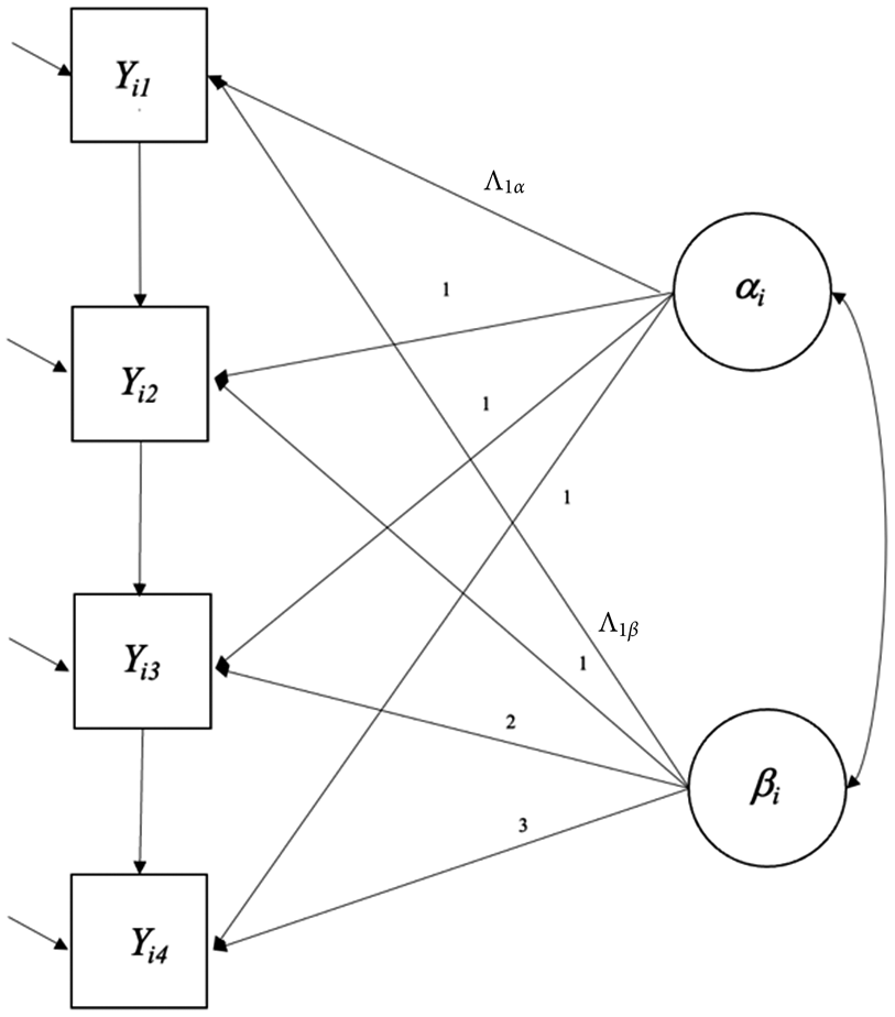

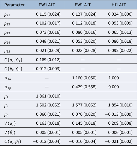

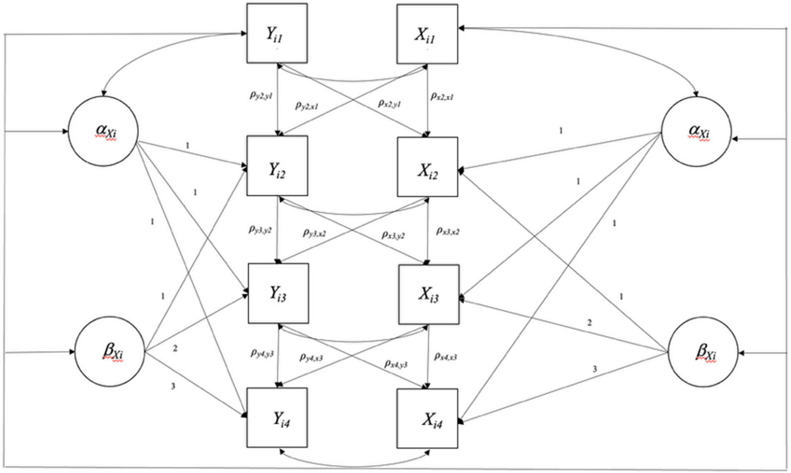


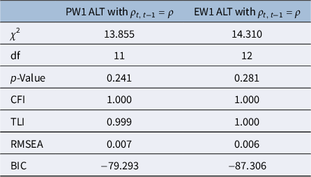
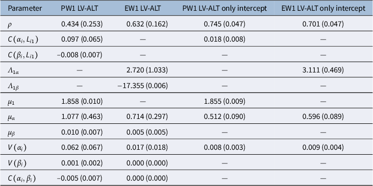
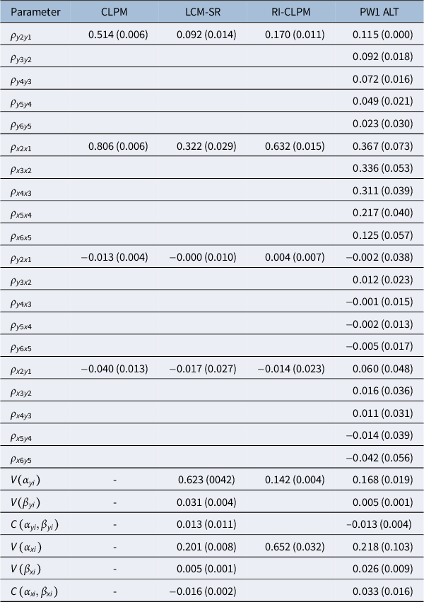
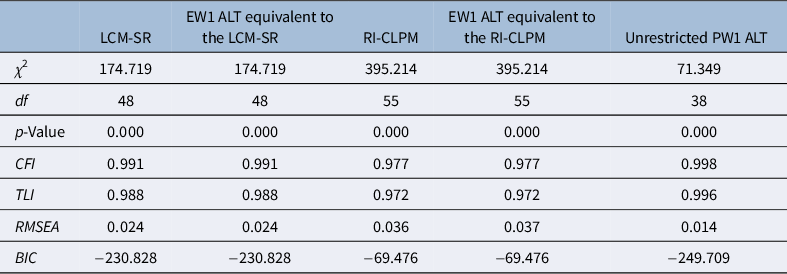
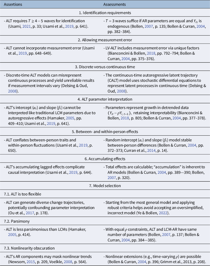


 Open access

